Privacy Aware Data Aggregation with Application in Voting Systems

1. Field of the Invention and Background

Turning raw data into informative insights is an essential procedure. When data is public, the aggregated information is trusted it can be reproduced. However, it is difficult to achieve trust when the data is private. An obvious example is the voting system where votes are kept in secret, yet everyone needs to trust the count. The problem is to achieve privacy and trust together.

Traditional paper-based voting satisfy privacy because the voter’s identity is detached from the ballot. However, trust is not satisfied. It relies on the fact that a considerable change in the count requires a large number of election staff to be involved (which is difficult to achieve). Apart from being expensive to perform, post-election protests show that paper-based voting is not trusted as claimed. Paper-based voting remains the only effective solution as it is much more difficult to address privacy-trust problem in electronic voting. Advanced technologies in digital security (i.e. homomorphic encryption, block chain, etc.) have been widely used to address this problem [1,2,3,4,5,6,7,8,9,10,11].

This article introduces a novel approach that satisfies both trust and privacy in the aggregation of private data. Tow implementations of the proposed approach for the voting system are also described. In the proposed method, each party encrypts its data and publishes the encrypted data publicly. Aggregation on encrypted data results in decrypted information without the need for decryption process.

2. Summary of the Invention

2.1. Simple Aggregation

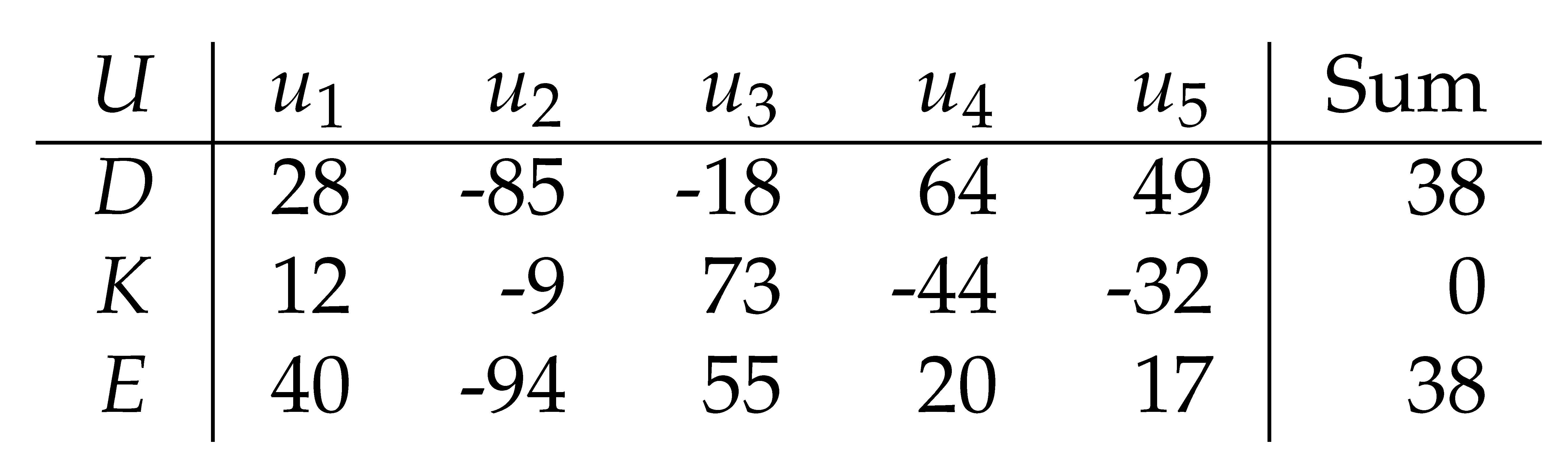
Although the voting system is the ideal example for the aggregation of private data, here a simpler example is used to better explain the proposed idea. In this example, there are five parties ($u_1$ to $u_5$) each producing a private number. They would like to find the sum of all private numbers without sharing them (e.g. to calculate the average). In Table 1, D is the list of private numbers (data) and K is the list of encryption keys. Each party encrypts the data by adding the encryption key to the data and publishes the encrypted data in E (i.e. $28+12=40$ for $u_1$). As shown in Equation 1, the sum of D is equal to the sum of E for any K if the sum of K is equal to 0 where $N=\left|U\right|$ is the number of parties (proven in Equation 2). Encrypted data (E) can be shared with all parties and used to calculate the aggregated information (sum of D) without revealing the actual data (D).

In the above example, each key ($k_i$) must be known only to the corresponding party ($u_i$). However, all parties need to ensure that the sum of K is equal to 0 and other parties perform encryption as expected. Implementing the key generation and encryption process is a challenging problem that is addressed later and in the context of voting systems (see Section 2.6). Assuming that the encryption process is done fairly, the proposed method satisfies trust and privacy together in data aggregation. Trust is satisfied as all parties can compute the aggregated information by sharing E. Privacy is satisfied as E does not reveal any information about the data (D) or encryption keys (K).

$$\sum _{i=1}^N{d}_i=\sum _{i=1}^N{e}_i\forall \sum _{i=1}^N{k}_i=0$$

(1)

$$\sum _{i=1}^N{d}_i=\sum _{i=1}^N{e}_i=\sum _{i=1}^N(d_i+k_i)=\sum _{i=1}^N{d}_i+\sum _{i=1}^N{k}_i=\sum _{i=1}^N{d}_i+0=\sum _{i=1}^N{d}_i$$

(2)

In the above example, if the sum of K is not equal to 0, the sum of D can be calculated as the sum of E subtracted by the sum of K. This is shown in Equation 3.

$$\sum _{i=1}^N{d}_i=\sum _{i=1}^N{e}_i-\sum _{i=1}^N{k}_i$$

(3)

The encryption key generation and encryption function depend on the aggregation function. Equation 4 shows another example in which the aggregation function is to find the product of all numbers. In this example, encryption is performed by multiplying $d_i$ by $k_i$ and the product of K is equal to 1. Equation 5 is the proof for Equation 4.

$$\prod _{i=1}^N{d}_i=\prod _{i=1}^N{e}_i\forall \prod _{i=1}^N{k}_i=1$$

(4)

$$\prod _{i=1}^N{d}_i=\prod _{i=1}^N{e}_i=\prod _{i=1}^N(d_i\times k_i)=\prod _{i=1}^N{d}_i\times \prod _{i=1}^N{k}_i=\prod _{i=1}^N{d}_i\times 1=\prod _{i=1}^N{d}_i$$

(5)

In the second example, if the product of K is not equal to 1, the product of D can be calculated as the product of E divided by the product of K. This is shown in Equation 6.

$$\prod _{i=1}^N{d}_i=\prod _{i=1}^N{e}_i÷\prod _{i=1}^N{k}_i$$

(6)

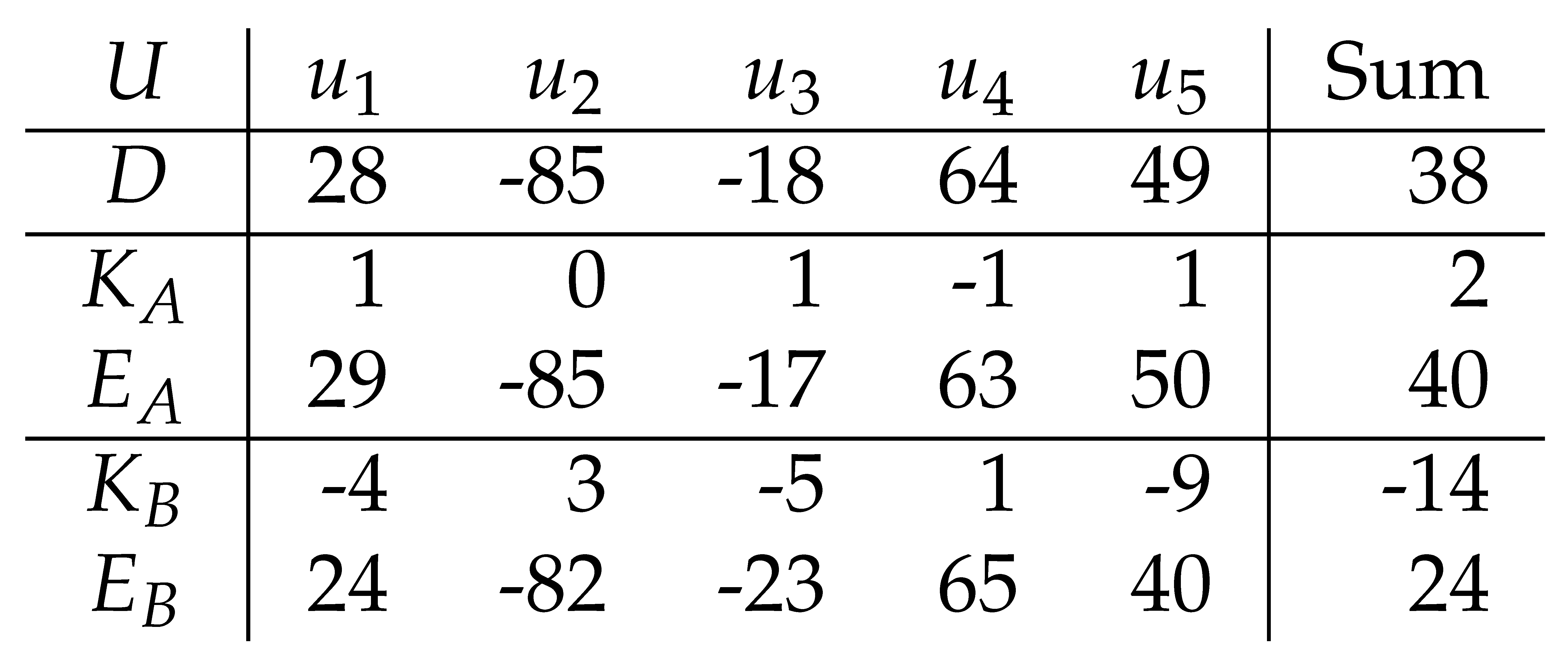
2.2. Randomness as Encryption Key

This section describes how randomness is used as an encryption key. Assume that the aggregation function is sum and the key generation logic is running on a trusted machine. A uniform random number generator with the range $-R$ to R can be used to generate a key for each party. If the number of parties (N) is known, the last key can be adjusted to ensure that the sum K is equal to 0. Otherwise, the sum of K is expected to be close to 0 since the distribution of K should resemble a symmetrical distribution around 0 (uniform randomness), especially when the number of parties increases. Since sum K is approximately 0, sum E is approximately equal to sum D.

R impacts the privacy of the data and the accuracy of the aggregated information. Table 2 demonstrates two examples in which $K_A$ and $K_B$ are produced with $R=1$ and $R=10$ and used to calculate $E_A$ and $E_B$, respectively. The smaller R (compare $K_A$ and $E_A$ with $K_B$ and $E_B$) results in less privacy as the original data (D) can be predicted with greater precision given the encrypted data (E). The smaller R also results in K being closer to 0 (i.e., the sum of E closer to the sum of D) In this situation R impact privacy and accuracy (trust).

In simple words, the idea is to mix data with randomness in such a way that the aggregation function eliminates randomness in the aggregated information. In other words, randomness is the encryption key and aggregation on the encrypted data results in the unencrypted information. The aggregation function determines how to use randomness to encrypt the data.

2.3. Voting System Aggregation

This section explains how to utilize the proposed method in a simple voting system. Assume that there are two candidates (Alice and Bob) and each individual can vote for one of the candidates. Also, there are two imaginary candidates (Red and Blue). Votes (for Alice and Bob) are transformed into imaginary votes (for Red and Blue) randomly given the probabilities matrix shown in Equation 7. Table 3 shows the encryption process. The key is generated using uniform randomness ranging from 1 to 10 (integer and inclusive). Alice is transformed to Red if the key is less than 8 (70% probability), otherwise to Blue (30% probability). Bob is transformed to Red if the key is less than 4 (30% probability), otherwise Blue (70% probability).

In the right-most column ’Counts’, the actual number of votes for Alice and Bob is assumed to be 600 and 400, respectively. The rest of the values in the count columns assume theoretical probability. Each number in key occurs exactly 100 times. Exactly 70% of Alice votes (420) and 30% Bobs votes (120) are turned into votes for Red. Also, exactly 30% of Alice votes (180) and 70% Bobs votes (280) are turned into votes for Blue.

$$P=\left[\begin{array}{ccc}& Red& Blue\\ Alice& 0.7& 0.3\\ Bob& 0.3& 0.7\end{array}\right]$$

(7)

The relation between the number of actual votes and imaginary votes forms a system of equations shown in Equation 8 that holds if theoretical probability is assumed (the name of the candidate or imaginary candidate stands for the number of votes). Equation 9 shows the same system of equations in the form of a matrix operation and explains how the number of votes for Alice and Bob can be computed using the number of votes for Red and Blue and the inversion of the probability matrix.

$$\left\{\begin{array}{c}0.7\times Alice+0.3\times Bob=Red\hfill \\ 0.3\times Alice+0.7\times Bon=Blue\hfill \end{array}\right.$$

(8)

$$\left\{\begin{array}{c}\left[\begin{array}{c}Alice\\ Bob\end{array}\right]\times \left[\begin{array}{cc}0.7& 0.3\\ 0.3& 0.7\end{array}\right]=\left[\begin{array}{c}Red\\ Blue\end{array}\right]\hfill \\ \left[\begin{array}{c}Alice\\ Bob\end{array}\right]={\left[\begin{array}{cc}0.7& 0.3\\ 0.3& 0.7\end{array}\right]}^{-1}\times \left[\begin{array}{c}Red\\ Blue\end{array}\right]\hfill \end{array}\right.$$

(9)

The imaginary vote (Red or Blue) is attached to voter’s identity and is published publicly without revealing the actual candidate (Alice or Bob). The number of vote for the actual candidate can be calculated given the number of votes for Red and Blue which are publicly available. Thus, the voting system satisfies both privacy and trust. Experimental probability adds an approximation to the equality in Equation 9. The approximation is discussed in Section 2.4.

Equation 10 generalize the above example for n candidates and imaginary candidates where $c_x$ and $i_y$ are the number of votes for candidate x and imaginary candidate y, respectively. $p_{x,y}$ is the probability that candidate x is transformed to candidate y

$$\left\{\begin{array}{c}\left[\begin{array}{c}{c}_1\\ c_2\\ c_3\\ ⋮\\ c_n\end{array}\right]\times \left[\begin{array}{ccccc}{p}_{c_1,i_1}& p_{c_1,i_2}& p_{c_1,i_3}& \cdots & p_{c_1,i_n}\\ p_{c_2,i_1}& p_{c_2,i_2}& p_{c_2,i_3}& \cdots & p_{c_2,i_n}\\ p_{c_3,i_1}& p_{c_3,i_2}& p_{c_3,i_3}& \cdots & p_{c_3,i_n}\\ ⋮& ⋮& ⋮& \ddots & ⋮\\ p_{c_n,i_1}& p_{c_n,i_2}& p_{c_n,i_3}& \cdots & p_{c_n,i_n}\end{array}\right]=\left[\begin{array}{c}{i}_1\\ i_2\\ i_3\\ ⋮\\ i_n\end{array}\right]\hfill \\ Simplified:C\times P=I\to C=P^{-1}\times I\hfill \end{array}\right.$$

(10)

The probability matrix (P) should be invertible (that is, the determinant of P is greater than 0). Also, there should be less than $n-1$ zero in each row or column (i.e. each candidate transforms to at least two imaginary candidates and at least two candidates to be transformed to each imaginary candidate). The second condition is set to maintain the privacy of the voters (i.e. votes for an imaginary candidate can not be linked to a specific candidate). Equation 11 shows a possible matrix that works for any number of candidates n where $\alpha >1/n$ and $\beta =(1-\alpha )/(n-1)$. Equation 7 is an example of such probability matrix where $\alpha =0.7$ and $\beta =0.3$.

It is possible to have more imaginary candidates than actual candidates. In that case, there are more equations than variables. However, P must be chosen such that the system of equations is solvable (i.e. the number of votes for the candidate can be computed given the number of votes for imaginary candidates).

$$P=\left[\begin{array}{ccccc}\alpha & \beta & \beta & \cdots & \beta \\ \beta & \alpha & \beta & \cdots & \beta \\ \beta & \beta & \alpha & \cdots & \beta \\ ⋮& ⋮& ⋮& \ddots & ⋮\\ \beta & \beta & \beta & \cdots & \alpha \end{array}\right]$$

(11)

2.4. $\alpha$ Controls a Tunable Trade-Off Between the Privacy and Trust

In the proposed matrix, each candidate is biased towards an imaginary candidate with probability $\alpha$. For example, Alice is biased to Red (Equation 7), which means that if an imaginary vote is Red, it is more likely that the actual candidate is Alice.

Equation 12 shows two other probability matrix $P_1$ and $P_2$ with extreme $\alpha$ (high and low, respectively). When $\alpha$ is high ($P_1$) almost all Red votes are contributed by Alice. This violates privacy of the voters, as anyone voted for Red is most likely to vote for Alice. When $\alpha$ is low ($P_2$) privacy is strongly satisfied (Red votes contributed by Alice and Bob almost equal). However, a lower $\alpha$ results in a lack of precision. This is experimentally shown in Section 2.5. $\alpha$ controls a tunable trade-off between privacy and trust.

There might be a probability matrix that increases both trust and privacy together. Also, in case votes are transformed so that the probabilities in P are exactly implemented (experimental probability is equal to theoretical probability), there would be no error in the system and $\alpha$ can be reduced to maximize privacy. Depending on the actual implementation of the voting system, it may be achievable at the cost of some dependencies in the system. This article assumes that each individual submits the vote independently at any given point in time.

$$\left\{\begin{array}{c}{P}_1=\left[\begin{array}{ccc}& Red& Blue\\ Alice& 0.99& 0.01\\ Bob& 0.01& 0.99\end{array}\right]\hfill \\ P_2=\left[\begin{array}{ccc}& Red& Blue\\ Alice& 0.51& 0.49\\ Bob& 0.49& 0.51\end{array}\right]\hfill \end{array}\right.$$

(12)

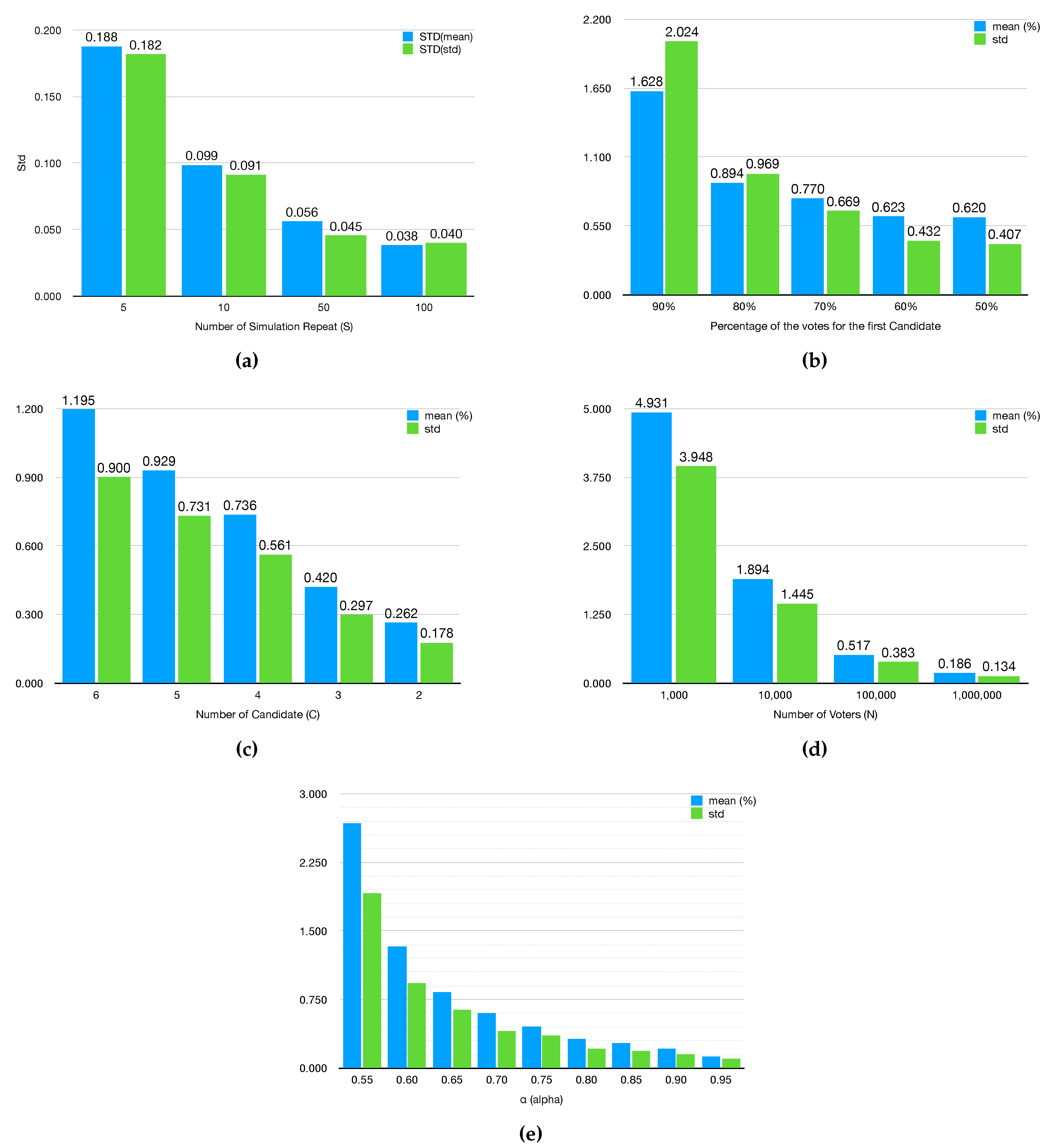
2.5. Experimental Analysis

In order to measure the accuracy of the system described in Section 2.3 a simulator is written in Python. The simulator takes the parameter listed below to perform a simulation and transforms each vote into an imaginary vote using a uniform random number generator. Finally, it compares the computed number of votes for each candidate with the real number of votes to see how much error is introduced due to randomness. The simulator calculates the percentage error rate for each candidate. For example, if the computed number of votes for Alice is 1100 and the actual number of votes is 1000, then the percentage error rate for Alice is $\left(\right(1100-1000)/1000)*100=10\%$. Since each simulation might be slightly different from the other (due to randomness), each simulation (for a given parameter) is repeated S times. Summary statistics are calculated for the percentage error rate of each candidate and also the percent error rate of all candidate combined. This report only presents the mean and standard deviation (std) of the percent error rate of all candidates combined as a measure of the precision of the system.

Parameters for each simulation include the followings

• N: Number of Voters
• C: Number of candidate
• V: Number of votes per candidate
• $\alpha$: As described in Section 2.3
• S: Number of reparations per simulation

Here, five experiments are performed, each of which demonstrates the effect of one of the above parameters by changing its value and performing the simulation. Table 4 summarise the value of the simulation parameter.

Experiment 1: Number of simulation repetitions

This experiment is to find out how many times the simulation needs to be repeated to ensure that the statistics on the percentage error rate are accurate. The number of repetitions (S) is varied between 5, 10, 50 and 100. The experiment is executed 10 times ($T_1$ to $T_{10}$). The standard deviation (STD) is calculated over the 10 experiments for both the mean and standard deviation (std) of the percentage error rate. Note that the capitol STD is used for the standard deviation over 10 executions of the experiment, and the lower case std is used for the standard deviation of the percentage error rate of S simulation repetitions. The results are shown in Table 5. Figure 1a shows the STD of both the mean and the std of the percentage error rate is reduced when the number of repetitions per simulation increases.

Experiment 2: Number of votes per candidate

This experiment studies the effect of the percentage of votes for each candidate on the percentage error rate statistic (over all candidates). 100,000 votes are distributed between two candidates where the first candidate takes 90% to 50% (with 10% intervals) of the total votes. As shown in Figure 1b, the lower error occurs when the candidate takes an equal number of votes.

Experiment 3: Number of candidates

This experiment shows the effect of the number of candidates on accuracy. The number of candidates ranges from 2 to 6. In addition, the number of voters increased to 1 million to prevent the lack of precision due to the lack of votes per candidate. To be fair, $\alpha$ is also varied to be $2\beta$ (that is, $(1/(C+1\left)\right)*2$). As shown in Figure 1c, the error rate was reduced as the number of candidates was reduced. The highest accuracy achieved with having only two candidates.

Experiment 4: Number of voters

This experiment shows that the error rate reduced as the number of voters increased. Figure 1d demonsterate the accuracy when the number of voters varies.

Experiment 5: The effect of $\alpha$

As mentioned in Section 2.4, the higher $\alpha$ results in higher accuracy (trust) but also reduces the privacy of the voter since each imaginary candidate strongly related to a specific candidate. Figure 1e shows the effect of $\alpha$ on the accuracy.

2.6. Implementation of Voting System

This section introduces two implementations of the voting system described in Section 2.3 after clarifying some key topics in relation to the implementation. The following data are involved when an individual acts to vote.

• C: The name of the candidate (option) the individual selected
• $ID$: The identity of the individual
• R: The random number used to transform the selected candidate (C) to an imaginary candidate (I)
• I: The imaginary candidate after transformation.

The goal is to prevent exposure of C and $ID$ together, as otherwise the privacy of the voter is violated. Instead, I and $ID$ must be public so that everyone can count the votes. Also, consider that R, I and $ID$ must not be exposed together as C can be computed given R and I.

Note that I should be generated based on the given probability matrix and uniform randomness, but not any other factor. However, C and R can be chosen in such a way that the resulting I is in favour of a specific candidate that is unfair. Since C is known to the voter, R must be generated by the system. The voter must expose C to the system without knowing R. However, the voter must know R is determined by the system before the voter exposes C to the system (i.e., the system provides a signature of R to the individual before C is provided).

Mechanical implementation

Imagine there are two candidates, Alice and Bob, and two fair dice, each corresponding to a candidate. Alice’s dice has four faces red and two faces blue. Bob’s dice has two faces red and four faces blue. There is no other mark on the dice. In the voting environment, voters throw the dice for the candidate of their choice (C) only once. The voting machine scans the color of the top surface of the dice (without knowing what dice is used) and publishes the colour (I) along with the voter’s identity ($ID$). This will perform the transformation of the candidate into an imaginary candidate with the probability matrix shown in Equation 13. From when the voters pick the dice to when the dice is returned to its initial place, the actual candidate selected by the voters C is exposed along with his identity $ID$. Thus, during this time, the voter must not be observed.

$$P=\left[\begin{array}{ccc}& Red& Blue\\ Alice& 2/3& 1/3\\ Bob& 1/3& 2/3\end{array}\right]$$

(13)

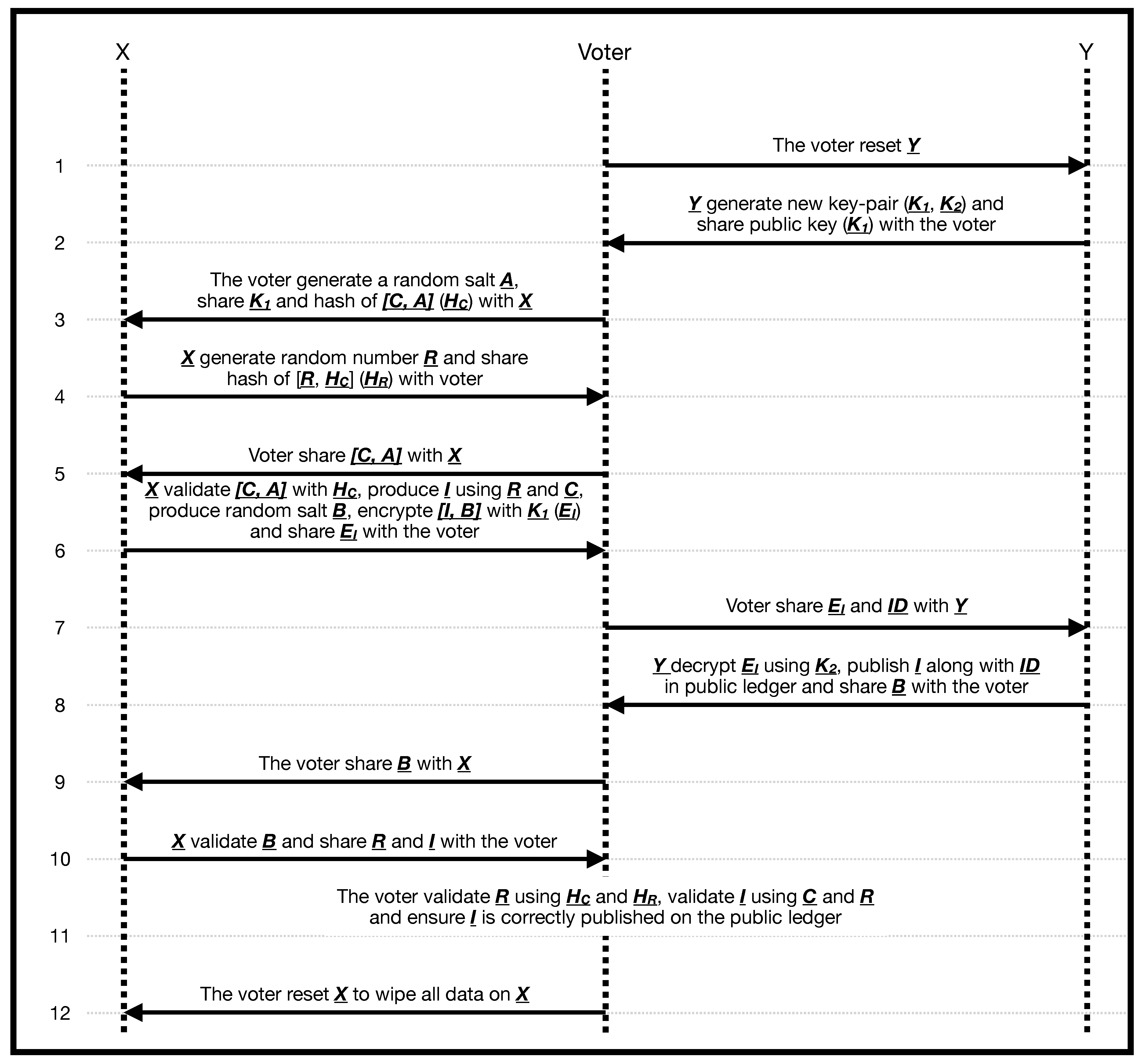
Digital implementation

Imagine there are two computers X and Y. X has limited input/output and does not have persistent memory (all data are wiped on restart). The voting actions are as follows and are shown in Figure 2:

• The voter reset Y
• Y generate new keypair ($K_1$, $K_2$) and share public key ($K_1$) with the voter.
• The voter generate random salt A and share $K_1$ along with hash of $[C,A]$ ($H_C$) with X
• X generate a random number R and share hash of $[R,H_C]$ ($H_R$) with the voter
• The voter shares $[C,A]$ with X
• X
  • validate $[C,A]$ using $H_C$
  • computes I given C, R and hardcoded probability matrix (known publicly)
  • produces a random salt (B)
  • encrypts $[I,B]$ using $K_1$ ($E_I$) and share it with the voter
• The voter provide the $E_I$ to Y along with voter’s identity $ID$
• Y decrypt I and publish it along $ID$ publicly.
• Y share B with the voter
• The voter provide B to the X
• when B is provided by the voter, X provides R and I to the voter.
• The voter validates R using $H_C$ and $H_R$ and ensures that I is calculated correctly.
• The voter resets X to wipe all its data.

Note that X observes the candidate selected by the voter (C) but not the identity of the voter $ID$. On the other hand, Y only observes I and $ID$. This ensures that C and $ID$ are never exposed to the same computer. There should be no communication channel between X and Y that can be used secretly without notified by the voter.