
Submitted:
22 January 2025
Posted:
23 January 2025
You are already at the latest version
Abstract
Parabolic leaf springs are components typically found in suspensions of freight railway rolling stock. These components are produced in high-strength alloyed steel, DIN 51CrV4, to resist severe loading and environmental conditions. Despite the material’s good mechanical characteristics, the geometric notches and high surface roughness that features its leaves might raise local stress levels to values above the elastic limit, with cyclic elasto-plastic behaviour models being more appropriate. In this investigation, the parameters of the Chaboche model combining the kinematic and isotropic hardening models are determined using experimental data previously obtained in strain-controlled cyclic tests. Once the parameters of the cyclic hardening model are determined, they are validated using a finite element approach considering the Chaboche cyclic plasticity model. As a result, the material properties specified in this investigation can be used in the fatigue mechanical design of parabolic leaf springs made with 51CrV4 (local approaches to notches and at surface roughness level) or even in other components produced with the same steel.
Keywords:
railway
; rolling stock
; parabolic leaf springs
; cyclic plasticity
; finite element analysis
; numerical optimization
1. Introduction
Over the years, engineers and researchers have developed more efficient geometries and processes to maximize the strength of suspension elements. Although leaf springs have been elements used for many years, these components have evolved both in terms of their resistance and geometries. The evolution of this component is also dependent on the type of sectors where these elements are inserted, as for example, road vehicles [1,2,3,4,5,6,7,8,9,10] and rail vehicles [11,12,13,14,15]. In the case of the railway freight sector, parabolic leaf springs (illustrated in Figure 1)) that are standardized by the International Union of Railways (UIC) [16] have gained higher representation due to their optimized geometry, which allows an increase in the specific energy storage capacity and reduction of the friction effects, which consequently increases the safety and quality of the wagon motion [17,18].
This two-axle freight vehicle suspension component is produced from high-strength steel, designated as 51CrV4 [19,20,21,22], which might be applicable in various industry machinery components in addition to road and rail suspension vehicles [23,24], such as steering knuckles, connecting rods, spindles, pumps, and gear shafts, pinions, forged crankshafts, and gears [21,25,26].
Despite the good mechanical resistance characteristics presented in several investigations [24,27,28,29], due the presence of geometric notches [18,30,31,32,33] and high surface roughness of its leaves (average up to = 7 m [34] and maximum roughness, = 40 m [35]), local stress levels can reach or exceed the yield limit of the material. Operating under these cyclic loading conditions, the cyclic elasto-plastic material behaviour model must be considered.
Over the years, different constitutive models have been developed to represent cyclic plastic behaviour. Some examples are the linear kinematic hardening model proposed by Prager [36], the multiple-yield surface model [37], two-surface plasticity model, yield and boundary surface model, [38,39], and others such as Malinin and Khadjinsky [40], Armstrong and Frederick [41], Chaboche [42], and Jiang [43]. In fact, the development of the cyclic plasticity models helped in the comprehension of the different mechanical responses associated with the plastic domain. Transient effects associated with Bauschinger’s effect, ratcheting, hardening or softening straining, as well as stress relaxation, are some of the examples observed and investigated more frequently in cyclic plasticity [42,44,45,46,47,48,49,50,51,52,53,54,55,56,57].
Some of these cyclic plasticity models have been used in numerical models to perform fatigue prediction analysis in cyclic elasto-plastic conditions for both smooth and notched components [58,59,60,61,62,63]. Even in components subjected to cyclic loadings below the yielding strength, due to the surface roughness, the localised plastic deformation may occur [64,65,66]. Under these conditions, cyclic plasticity should be considered for fatigue crack initiation analysis. Moreover, in fatigue crack propagation analysis, there is localised plasticity at the crack tip. Thus, plasticity models should also be considered in determining the cyclic material behaviour at crack tip [67,68,69,70].
In this investigation the Chaboche model, widely used for designing structural components under cyclic loading, is considered. The Chaboche model considering the effect of combined kinematic and isotropic hardening is calibrated using the experimental data on 51CrV4 martensitic steel, obtained in strain-controlled fatigue tests. This combination of kinematic and isotropic hardening models has been widely used in different works, resulting in good prediction results compared with experimental data [45,71,72,73]. The parameters of the Chaboche kinematic hardening model are calibrated considering the stabilised cyclic elastoplastic Ramberg-Osgood curve for 90% of the total life of the specimens. Regarding the isotropic hardening model parameters, these are calibrated considering the material softening amount curve ([74]) and the curve of variation in the size of the normalized elastic limit surface throughout the test. In the parameter calibration procedure, the Hager-Zhang’s conjugate gradient unconstrained optimization method was considered. To validate the estimated combined hardening parameters, the estimated parameters are used in the numerical computation using an elasto-plastic finite element approach. The outcomes by numerical model are subsequently compared with experimental data and the comparison errors are determined.
2. Cyclic Elasto-Plasticity for Steels
2.1. Elasto-Plasticity Modelling
Cyclic plasticity, a crucial factor in fatigue analysis, is examined for components subjected to loads exceeding the material’s yield strength. The Chaboche hardening model [42] is used to characterize this cyclic behaviour. This model is based on the yield von Mises plasticity criterion, as outlined below
with and R denoting, respectively, the initial size of the elasticity limit surface and the change in the size of the elasticity limit surface. If , the elasticity limit surface expands, otherwise, F contracts. Concerning the stress tensors, and denoting respectively the deviatoric part of the stress tensor, , and the back stress tensor, .
The direction of plastic flow is determined by the associative flow rule, which follows the principle of normality, such as
where denotes the time rate of plastic strain tensor. The consistency condition, , serves as the condition for updating the stress and strain-state variables, with assuming , , or R. The plastic multiplier in Equation (2), is determined from the consistency condition, which ensures the Kuhn–Tucker conditions.
2.2. Kinematic Hardening Model
In several investigations, the cyclic hardening behaviour, mainly in steels, has been modelled by the Chaboche hardening model. Chaboche kinematic hardening was developed considering the von Mises plasticity criterion (Equation (1)). As advantage, Chaboche model can predict the transient effects such as cyclic hardening or softening, ratcheting, mean stress relaxation, etc. Chaboche kinematic hardening model is an improved model from Amstrong and Frederick, AF model, which itself is an improved model from the linear hardening rule [36], developed by Prager [36], by introducing the concept of dynamic recovery [41] . Thus, the back stress tensor, , is given by a sum of i-th component of back stress tensor, , such that [42]
and the variation of each individual back stress tensor, , is
In equations (3) and (4), and are fitting parameters and denotes the effective plastic strain rate, which is given by
The Chaboche kinematic hardening model permits overcome some constraints pointed out by Prager and AF models, such as the difficulty of a accurate behaviour representation for large deformation regimes, and the transition from elastic to plastic regimes [42]. Several investigations have proved that considering only three components can reach good predictions ratcheting behaviour [42,55].
2.3. Isotropic Hardening Model
Although the Chaboche hardening model is modeled for material behaviour with kinematic hardening, it can be considered with isotropic hardening. The isotropic hardening that represents the change in the size of the elasticity limit surface, , is given by
where denotes the rate of isotropic hardening and denotes the saturation of isotropic hardening. Both and are parameters depending on the material and temperature. Lower values of indicate a slower saturation of the model, whereas for materials exhibiting a high value of , its yield surface will to evolve very fast cycle-by-cycle. Integrating the Equation (6) results that
Equation (7) provides the size of the elasticity limit surface, which may be considered for both in monotonic and cyclic loading conditions.
2.4. Empirical Estimation of Hardening Variables
The estimation of kinematic and isotropic hardening variables is normally carried out considering test data under strain-controlled cyclic loading conditions. Under these conditions, the kinematic hardening is represented by equation (8) as [42]
where the parameters and are determined by fitting the Equation (8), and denotes the variation of the elasticity limit surface for the stabilized-state hysteresis loop. Equation (8) allows taking into account both the ratcheting effect and the stress saturation effect [42,75]. According to some research, the limit stress stabilised cyclic curve is reached for strain amplitudes of 2% and 3% in high-strength steels, which means that after 2% and 3%, the increase of stress amplitude with the strain amplitude is quite low [76,77,78]. This slight increase of hardening stress may be considered summing to the equation (8) a linear component of stress, given by Prager’s model, which results in
The fitting of the parameters and can be carried out considering the hysteresis loop in stabilized conditions for the largest strain amplitude analysed, or by the elasto-plastic cyclic curve. According to the literature [42,74,79,80], the Ramberg-Osgood, RO, model is one of the most suitable model for fitting the Chaboche’s parameters in steel materials. The RO model is a stable elastic-plastic hardening that relates the total strain amplitude, , to the stress amplitude, , through a power law, of the form [81], such that
where E is the Young’s modulus, is the cyclic hardening strength coefficient, and is the cyclic strain hardening exponent. Ramberg–Osgood’s model (Equation (10)) is given by decomposing the total strain amplitude, , into its elastic, , and plastic, , parts. In spite of being an ancient model, several researchers [24,74,82,83,84,85,86,87,88] recently used this equation model (10) to characterize the elasto-plastic behavior of a material under cyclic loadings. , Also, data obtained from strain-controlled cyclic testing, the parameters of the evolution of the elasticity limit surface (equation (7) can be obtained. Thus, the elastic limit surface (equation (7) can be represented in terms of the normalized maximum stress, as a function of the accumulated plastic strain, such that
with , , and denoting the maximum stress corresponding to the first cycle, the stabilized cycle, and the i-th cycle, respectively. denotes the difference between the value of yielding stress in the stabilized cycle and the value of yielding stress in the first cycle. relies on the imposed strain amplitude. Increasing the total strain amplitude, the amount of hardening/softening, , increases with the maximum value, . In several investigation [76,77,78], it was found that for medium and high strength steels, the variation in the elasticity limit surface remain unchanged for around 2 or 3 % of applied strain. varies with the applied strain amplitude, , through a decreasing power law, written as [89]
where parameters and are estimators for the amount of cyclic softening. This approach can be considered because increasing the total strain amplitude, the amount of hardening/softening, , tends to increase up to the maximum value, . can be estimated for applied strain amplitude values around 2% or 3% for medium and high strength steels [76,77,78].
3. Material and Analysis Procedure
The calibration of the cyclic behaviour of the steel under investigation, 51CrV4, is carried out considering two approaches, experimental and computational. In the experimental approach, data collected from cyclic tests are used to estimate kinematic and isotropic hardening parameters, using statistical fitting models. The estimated parameters are considered in the computational models in order to compare and validate the Chaboche model for 51CrV4 spring steel applied to parabolic leaf springs of railway freight wagons.

Table 1.
Standard chemical composition of 51CrV4 steel grade in % wt .
| Material | C | Si | Mn | Cr | V | S | Pb | Fe |
|---|---|---|---|---|---|---|---|---|
| DIN 51CrV4 (1.815) | 0.47-0.55 | ≤0.40 | 0.70-1.10 | 0.90-1.20 | ≤0.10-0.25 | ≤0.025 | ≤0.025 | 96.45-97.38 |
3.1. Chemical Composition and Microstructure
51CrV4 steel is a chromium-vanadium alloyed steel with an average carbon content of 0.50%, approximately. When used in parabolic leaf springs, 51CrV4 steel follows the heat treatments described in ISO 683-14 standard [22], which consists of quenching at 850 oC in an oil bath and then tempering at 450 o W . As a result, 51CrV4 presents a microstructure of quenched martensite with retained austenite (white phases) as shown in Figure 2[92].
The heat treatment provides the 51CrV4 steel its high mechanical strength. According to the material characterization tests carried out in [24] under monotonic loading conditions, following the ISO 6892-1 [93] standard, the spring steel exhibits a yield strength, = 1271.48 MPa, an ultimate tensile strength, = 1438.5 MPa, a (conventional) ductility at fracture, = 7.53 %, and a Vickers hardness of 447 HV. Table 2 presents the summary of the 51CrV4 mechanical properties, with E denoting the Young’s modulus and , the area of reduction at fracture.
3.2. Experimental Procedure and Statistical Techniques
Kinematic and isotropic mechanical properties are to be determined for chromium-vanadium alloyed steel. The cycle tests carried out in [24] are considered to determine the cyclic hardening properties and subsequent verification in the computational model by analysing the hysteresis loops. The sample set consists of seven flat-shaped specimens with a net cross-section, , of 38.98 ± 0.28 mm2 whose width, , is mm and thickness, , is mm (see Figure 3 - B) (see Table 3).
The specimens were manufactured and tested under constant strain-controlled amplitude loading conditions according to ASTM E606 standard [94] for a strain ratio, and an average strain rate d/dt of 0.8 %/s. The applied strain amplitudes were 0.375 (), 0.50 (), 0.750, 1.00, and 1.25 %. The cyclic tests were conducted in an INSTRON 8801 servo-hydraulic machine with a load cell of 100 kN, with a dynamic INSTRON 2620-202 clip gauge with a working range of ± 2.5 mm (see Figure 4).
The kinematic and isotropic hardening properties are estimated using statistical techniques based on the least-squares method. In the case of the problem can be described by a linear function, the ordinary least-squares (OLS) is considered, whereas if the problem is non-linear, an unconstrained numerical optimization scheme is assumed.
For a linear response function, then
with and denoting the design vector and respective response, respectively [95]. The minimization problem results in the equation system in (15), with
where is the design matrix, and is its transposition. is the estimator vector containing estimators, which in this case is and .
On the other hand, for a non-linear response function, the objective function
with denoting the size of vector is assumed. The minimization numerical problem is solved using the iterative method of Broyden–Fletcher–Goldfarb–Shanno (BFGS), with the recurrence equation given by [96]:
where in each iteration, k, the search direction, , is obtained using Hager-Zhang’s conjugate gradient method [97], for a maximum convergence error of 1.00 × 10⁻⁵. The gradient of the objective function for x is computed using forward-mode automatic differentiation [98] and the step size, , is always positive and assumed to be 1.0. With respect to the initial guess for a hessian matrix , this one is the identity matrix.
3.3. Computational Approach
A computational approach using finite element analysis (FEA) in ANSYS software was adopted to verify the cyclic material properties derived from the statistical analysis of the experimental data. A pure-displacement finite element formulation was considered for a cyclic small elasto-plastic deformation analysis of the material. The system of differential equations was solved incrementally by applying a displacement increment, , according to the Newton-Raphson procedure (with the L2-Norm), and using the direct sparse method with LDLT factorization for the matrix equation (18),
with denoting the external forces applied at nodes, representing the restoring loading vector, and denoting the symmetric and positive-definite global tangent matrix.
A single quadratic 20-node iso-parametric finite element with dimensions following a full integration scheme of Gauss was assumed. The von Mises plasticity criterion combined with the Chaboche (kinematic plus isotropic) hardening model [42] was considered in the integration of the plasticity law, via the return mapping algorithm, according to the Euler backward implicit scheme [99,100,101]. The finite element simulates the material behaviour under a uniformly distributed strain condition, by considering isostatic boundary conditions.
4. Results and Discussion
4.1. Cyclic Behaviour
Cyclic tests were performed until failure as illustrated in Figure 5. In research carried out in [24], it was found that 51CrV4 steel exhibits cyclic softening behaviour. Figure 5 shows the hysteresis loops for the 1st cycle and the cycles corresponding to 50 and 90 % of the total life. The consideration of the hysteresis loop for 50% of the total life is widely used for the development of fatigue resistance curves, however the 51CrV4 steel revealed in the analysis in [24] that for high strain amplitude conditions (higher strain amplitudes than 0.5 %), the hysteresis loops do not stabilise completely, which is also proven by Figure 5, with a continuous cyclic softening and mean stress relaxation, however the differences and variations are quite low. Thus, in the analysis of the elasto-plastic transient given by the isotropic and kinematic cyclic laws for a life of 90% of the total life is considered. Assuming 90 % of the total life, it is still ensured that the hysteresis loops do not consider the final loops containing crack initiation and propagation phenomena.
4.2. Determination of the Kinematic Hardening Properties
When determining the kinematic hardening parameters, hysteresis loops for a life of 90% are considered. The hysteresis loops for a 50% of the total life are also used considered, but only for comparison. Thus, considering the RO cyclic curve (equation (10)) for 90% of total life, cyclic RO parameters of MPa, and with a coefficient of determination, are obtained. The kinematic hardening properties are determined by fitting the curve of equation (9) to the cyclic RO curve (equation (10)), using the unconstrained numerical optimization scheme previously described, where in equation (16), such that
and
with number of back stress, . The selected model was the model that provided the highest minimization of the objective function, hence the smallest , the smallest number of back stress, and that ensured the condition, and and with . As a result of this condition, the selected Chaboche’s kinematic model is constituted by 4 back stresses (3 non-linear and 1 linear).
Since the optimal solution is dependent on the input parameters, the process to obtain the best initial design vector, , with , is made from the generation of a random sample. The generation of the random values is made using a pseudo-generator of random values designed as Mersenne Twister that is a twisted GFSR random number generator of 32 bits MT19937 [101,102]. Side bounds are introduced in the model to constrain the regression parameters and . The lower and upper side bounds are assumed to be respectively for both parameters, and . Parameters are fitted until the value of fracture strain, . Notice that the fourth back stress is linear in order to take into account the effect of ratcheting and mean stress relaxation effect [45].
Considering the Chaboche parameter fitting method for 4-back stress kinematic hardening models (3 nonlinear and 1 linear), the optimal parameters are MPa, , MPa, , MPa, , and MPa, with a relative root mean square, , from 0.2853 %. The value of each fitting parameter, and is presented in Table 4.
Figure 6 depicts the decomposition of total the back stress tensor, , in the model with 3 non-linear, , , and and 1 linear, components. From Figure 6 - Right, it is notable that there is a good agreement between the variation of back stress components with the the assumptions of Chaboche’s model. and have higher impact in the initial hardening until 2 % of the plastic strain amplitude. On the other hand, contributes gradually to increase the kinematic hardening from the beginning of the plastic deformation process. Lastly, increases linearly the total back stress tensor. In addition, Figure 6 - Left compares the decomposition of total stress, , into the total back stress, , and the size of elasticity limit surface.
In case hysteresis loops of 50 % of the total life were chosen, the RO cyclic curve described with MPa (more 4.09 %), (more 16.20 %), and of 731.5 MPa (less 7.49 %) results in MPa, , MPa, , MPa, , and MPa (presented in Table 4), whose highest differences occur for constants and . Note that in the case where the RO cyclic model parameters were fitted by estimation models using monotonic properties, for example the Modified Universal Slopes method, MUSM, (with coefficients MPa, exponents = -0.09 and = -0.56 [103]), results in MPa, , MPa, , MPa, , and MPa, with a of 0.3167%, and a cyclic yield strength MPa (which results in a variation in the size of the elastic limit surface, = -510.1 MPa). Comparing both Chaboche kinematic data, it is verified that the constants C are in the same order of magnitude, except the constants . These constants obtained from the experimental data at tend to be lower than (MUSM method). The highest reduction occurred in , which is responsible for the first hardening zone, which along the way is the zone most affected by the parameter .
4.3. Determination of the Isotropic Hardening Properties
The isotropic hardening law properties, and , in equation (6) are determined separately. Initially the parameter is determined and subsequently is determined, both using the unconstrained optimization scheme.
Considering the determination of the isotropic hardening parameters following the unconstrained optimization scheme for the variation of , (equation (12)), then, in accordance with equation (16), it is assumed that
and
In the numerical procedure, the lower and upper bounds of regressors, , , and are found. After finding the side bounds, a pool of permissible solution of regressors is created in order to be considered as the initial design vector, . From a pool of optimal solutions, the best optimal solution is considered. It is assumed as the best optimal solution, the solution that has the lowest value of the objective function. According the algorithm, the optimal solution of is MPa , = - 380.55, and , with a relative root mean square error, .
Figure 7 depicts the evolution of the amount of cyclic softening as a function of the applied strain amplitude. According to this variation, the existence of a cyclic softening is considered after a threshold strain value, . The threshold strain, corresponds to the strain for a stress of 648 MPa, which is approximately equal to the cyclic yield strength, = 676.7 MPa, but 4.24 % inferior. From Figure 7, it is verified that is reached after 2.0 % of strain amplitude, which is in accordance with [76,77,78].
Regarding the isotropic saturation rate parameter, , its value is determined according to the method in [42,90,91], such that the response curves are assumed to be
and
Figure 8 depicts the normalized variation of the yield surface size evolution, , throughout the cyclic testing until 90 % of the total life to failure. Both the mean curve and standard deviation bands concerning the mean value of are also presented. From the comparison between experimental data and numerical outcome, it is notable that cyclic tests performed at exhibited a no-coherent evolution, due to its large differences in rate size evolution. In contrast, cyclic tests carried out at higher strain amplitudes than exhibited a better agreement with respect to the numerical approach.
Considering the 90% of total-life criterion, most cyclic tests appear not to have an actual stabilization plateau as suggested by numerical approach [42]. However, one of the cyclic tests, at appears to have a stabilised state. With respect to the quality of the fitting curve, it is noted that in the initial cyclic softening phase, from until 1, the regression curve tends to exhibit a lower saturation rate whereas in the middle phase, the softening evolution follows the same trend than the experimental results. This behaviour has been also found in some materials [90,104]. The average value found for was 0.3705 with a of . According to [90], is usually assumed to be between 50 and 0.5 considering the half-life criterion. In spite of being slightly lower than 0.5, represents the average value obtained from different tests for a full cyclic test. The high value of is related to the shape of the softening evolution curve. In order to reduce the value, other isotropic hardening models contemplating an improvement in the stabilization rate and the shape of the softening/hardening evolution curve may be considered [104,105].
4.4. Cyclic Elasto-Plastic Response Using a Computational Approach
After determining the best fitting for the kinematic and isotropic hardening parameters, the numerical model following the finite element method approach as described previously, with the respective elasto-plastic mechanical properties presented in Table 5 is considered and compared with the experimental results to validate the cyclic plasticity model of chromium-vanadium steel 51CrV4.
For each strain amplitude condition, enough number of cycles were applied such that the stabilised behaviour will be possible to observe. The adopted strain ranges were only 1.00, 1.50, 2.00, and 2.50 %. For strain ranges inferior than 1.00 % it is observed a elastic hysteresis loops after the first cycles, and therefore the strain level of 0.75% was not considered for the analyses.
In a first phase, the hysteresis loops of the material numerical model were evaluated by comparing the first cycle and the cycle associated with the loop corresponding to 90% of the total life. The higher strain ranges were considered for the first analysis. Figure 9 depicts the comparison between experimental data in the first and stable hysteresis loops with the numerical outcomes in terms of stress and applied total strain for the presented strain amplitudes.
From the analysis of the monotonic part, it is noted the existence of a lag in the initial hardening between experimental and numerical outcomes. This lag is associated with the definition of the isotropic hardening law, such that the linear hardening coefficient (as described in the Voce’s law) was assumed to be null and also due to the material plastic properties variability. On the other hand, the maximum stress for each applied loading level tends to be very close between the models as illustrated in Figure 9, Figure 9, and Figure 9. In the case of Figure 9, it is verified that the yield strength is much higher than the others, generating a higher difference associated with the hardening material. However, this difference tends to remain constant since the experimental and numerical curves tend to be collinear.
Comparing the hysteresis loops associated with the first cycle, it is visible that the plasticity model cannot describe correctly the lower branch of the experimental model. This plasticity model imprecision is verified in both the three highest applied strain levels. However, comparing the experimental data associated with the first and steady-stable loops is notable that the evolution of the minimum stress is much less than the maximum tensile stress. This behaviour is typical for material exhibiting a non-Masing behaviour [58]. The variation of maximum stress in each cycle for data under analysis is presented in Figure 10. This figure clearly shows the existence of a non-symmetry associated with the maximum and minimum stress in each cycle of the softening process. In fact, the variation of the minimum stress of the hysteresis loop seems to be only associated with the kinematic hardening component for any applied strain range. This minimum stress tends to remain unchanged throughout the life of the specimen regardless of the applied strain range.
Concerning the effect of the isotropic saturation rate parameter, , it is shown that the plasticity model with an average value of equal to 0.37 cannot describe correctly the first phase of the material softening for the higher strain ranges. However, for a strain range of 0.5 %, there is a good correspondence between the experimental and numerical behaviour for the maximum stress in each cycle. Notice that is an average value assumed constant for several strain amplitudes and throughout the cyclic life. Therefore, despite this value not corresponding to the reality of the material model, = 0.37 appears to be conservative for most of the whole life as illustrated in Figure 10.
Now, analysing the hysteresis loops in the steady-state conditions, one verifies that the maximum and minimum stress of the hysteresis loops are very similar compared with experimental data. In general, for higher applied strain ranges, as presented in Figure 9 and Figure 9, the maximum stress tends to be around 6.0 % superior, whereas, for the testing condition in Figure 9, the maximum stress is slightly inferior, around -4.0 %, in face to the experimental data (see Figure 11). Concerning the minimum stress, the offset of the numerical models is around -10.0 % as seen in Figure 11. The maximum deviation occurs between 5 and 30 % of the total-life and they can achieve 16 %. For specimens tested with a strain amplitude of 0.5 %, a different error analysis needs to be made. In fact, analysing Figure 9 it is verified that from the first cycle until the stabilised cycle, the strain ratio of is never achieved. Over this assumption, the error associated with the minimum value of the stress at the stabilised cycle is normal being above 100 % as seen in Figure 10. Concerning the hysteresis loop area of , one verifies that the area obtained from numerical outcomes tends to be conservative.
5. Conclusions
The modelling of the elasto-plastic behaviour in cyclic conditions of the chromium-vanadium alloyed steel (DIN 51CrV4) was obtained in this paper. The experimental data concerning the cyclic tests performed previously in [24] were used for determining the parameters of the isotropic and kinematic hardening plasticity model. Chaboche’s kinematic hardening model along with isotropic hardening model were considered for modelling the cyclic behaviour. The hardening model parameters were obtained from statistical techniques based on the least-squares method. These parameters were considered in the finite element model whose outcomes were posteriorly compared to the experimental results.
Initially, the Chaboche’s kinematic hardening properties for stabilised cyclic conditions assuming 90 % of the total life criterion were determined. The Ramberg-Osgood’s elasto-plastic parameters were used for fitting the kinematic coefficients and . The best fit was found for three non-linear and one linear back stress, with values of MPa, , MPa, , MPa, , and with a of 0.2853 %. These values were posteriorly compared with the ones obtained from stabilised cyclic conditions for a 50 % of the total life since this criterion is usually used for determining the fatigue life in strain-controlled life. Comparing both criteria, one verified that both criteria may be used without existing large differences in the estimators and , although the cyclic strength tends to decrease. Additionally, Chaboche kinematic hardening properties were estimated from estimation models based on monotonic properties, the modified Universal Slopes (MUSM), which does no affected significantly the kinematic coefficients if the cyclic yield stress is defined correctly.
Concerning the isotropic hardening parameters, the evolution of the yield surface, R, was determined for several strain ranges. A relationship for estimation of as a function of the applied strain amplitude is assumed. According to the relative root mean square error, a regression model with less than 15 % was found. In addition, a limit value for was found () from the regression model. This value, , is independent of the applied strain range and is equal to -232.2 MPa. Regarding the isotropic saturation rate, , from the optimization methods was found an average value of 0.3705 with a = 42.00 %. The high value of was associated with the large scatter verified for different strain amplitudes and the low fitting of throughout the test.
From the final comparison between the fitting of the constitutive model in transient conditions was verified that the non-Masing material behaviour does not allow the lower branch of the stress of the hysteresis loops to be represented with accuracy. The average value for rate saturation, , may be used as a conservative value for the maximum and minimum stresses with deviation around 10 and 20%. The area of the hysteresis loops obtained at the end of each test is slightly larger than the experimentally verified and therefore conservative. For lower strain amplitudes and close to the elastic limit, the plasticity model presents certain difficulties in representing the shape of stress-strain hysteresis loops. Furthermore, the use of the parameter fails to represent the effect of isotropic softening since it is twice as high as that observed experimentally. Under these conditions, the offset can be significant.
In summary, in the investigation carried out, it was possible to determine the kinematic and isotropic hardening parameters based on the Chaboche plasticity model with good accuracy for the highest strain amplitude levels. For low strain amplitude levels, close to the yield limit zone, it is recommended to use the model with caution due to the observed offsets in the comparison analysis, although these offsets make the model more conservative.
Author Contributions
Conceptualization, Gomes V.M.G.; methodology, Gomes V.M.G.; software, Gomes V.M.G., Dantas, R.; validation, Gomes V.M.G., Dantas, R., de Jesus A.M.P.; formal analysis, Gomes V.M.G.; investigation, Gomes V.M.G., Dantas, R.; resources, Correia J.A.F.O. and de Jesus A.M.P.; data curation, Gomes V.M.G.; writing—original draft preparation, Gomes V.M.G.; writing—review and editing, Gomes V.M.G., Dantas, R., Correia J.A.F.O., and de Jesus A.M.P.; visualization, Gomes V.M.G.; supervision, Correia J.A.F.O., and de Jesus A.M.P.; project administration, de Jesus A.M.P.; funding acquisition, Correia J.A.F.O. and de Jesus A.M.P.
Funding
This research received no funding.
Institutional Review Board Statement
Not applicable.
Informed Consent Statement
Not applicable.
Data Availability Statement
The data presented in this study are available on request from the corresponding author. The data are not publicly available due to privacy or ethical restrictions.
Acknowledgments
The authors also want to express a special thanks to the Doctoral Programme iRail - Innovation in Railway Systems and Technologies funded by the Portuguese Foundation for Science and Technology, IP (FCT) through the PhD grant (PD/BD/143141/2019); and the following Research Projects: FERROVIA 4.0, with reference POCI-01-0247-FEDER-046111, co-financed by the European Regional Development Fund (ERDF), through the Operational Programme for Competitiveness and Internationalization (COMPETE 2020), under the PORTUGAL 2020 Partnership Agreement; SMARTWAGONS - DEVELOPMENT OF PRODUCTION CAPACITY IN PORTUGAL OF SMART WAGONS FOR FREIGHT with reference nr. C644940527-00000048, investment project nr.27 from the Incentive System to Mobilising Agendas for Business Innovation, funded by the Recovery and Resilience Plan and by European Funds NextGeneration EU; and PRODUCING RAILWAY ROLLING STOCK IN PORTUGAL, with reference nr. C645644454-00000065, investment project nr. 55 from the Incentive System to Mobilising Agendas for Business Innovation, funded by the Recovery and Resilience Plan and by European Funds NextGeneration EU. The authors also want to express their thanks to the Python, Julia, and Ansys communities.
Conflicts of Interest
The authors declare no conflict of interest.
References
- Kam, T.Y.; Arora, V.K.; Bhushan, G.; Aggarwal, M.L. Fatigue Life Assessment of 65Si7 Leaf Springs: A Comparative Study. The Scientific World Journal, Hindawi Publishing Corporation 2014, pp. 365–370. [CrossRef]
- Kong, Y.; Omar, M.; Chua, L.; Abdullah, S. Explicit nonlinear finite element geometric analysis of parabolic leaf springs under various loads. The Scientific World Journal 2013, 2013. [CrossRef]
- Krason, W.; Hryciow, Z.; Wysocki, J. Numerical studies on influence of friction coefficient in multi-leaf spring on suspension basic characteristics. In Proceedings of the AIP Conference Proceedings. AIP Publishing LLC, 2019, Vol. 2078, p. 020049.
- Krason, W.; Wysocki, J.; Hryciow, Z. Dynamics stand tests and numerical research of multi-leaf springs with regard to clearances and friction. Advances in Mechanical Engineering 2019, 11, 1687814019853353. [CrossRef]
- Zhao, W.Y.; Wei, L.; Wang, J.F.; Wang, J.; Gu, X.S.; Song, C. Study on the modeling method of leaf spring based on assembly pre-stress. Advanced Materials Research 2013, 663, 545–551. [CrossRef]
- Husaini.; Ali, N.; Riantoni, R.; Putra, T.E.; Husin, H. Study of leaf spring fracture behavior used in the suspension systems in the diesel truck vehicles. IOP Conf. Series: Materials Science and Engineering 541 2019. [CrossRef]
- Husaini.; Anshari, R.; Ali, N.; Yunus, J. The analysis of the failure of leaf spring used as the rear suspension system in 110 PS diesel trucks. 2023, p. 012046. [CrossRef]
- Fuentes, J.; Aguilar, H.; Rodríguez, J.; Herrera, E. Premature fracture in automobile leaf springs. Engineering Failure Analysis 2009, 16, 648–655. https://doi.org/Paperspresentedatthe24thmeetingoftheSpanishFractureGroup(Burgos,Spain,March2007.
- Husaini, H.; Farhan, M.; Ali, N.; Putra, T.E.; Anshari, R.; Suherman, K. Analysis of the Leaf Spring Failure in Light Duty Dump Truck. Key Engineering Materials 2022, 930, 43–52. [CrossRef]
- Deulgaonkar, V.R., R.M.K.S.; Mandge, A.; Patil, A.; Makode, A. Failure Analysis of Leaf Spring Used in Transport Utility Vehicles. J Fail. Anal. and Preven 2022, 22, 1844–1852. [CrossRef]
- Chen, Y.H.; Chen, G.C.; Wu, C.T.; Lee, C.L.; Chen, Y.R.; Huang, J.F.; Hsiao, K.H.; Lin, J.I. Object investigation of industrial heritage: The forging and metallurgy shop in Taipei railway workshop. Applied Sciences 2020, 10, 2408. [CrossRef]
- Matej, J.; Seńko, J.; Awrejcewicz, J. Dynamic Properties of Two-Axle Freight Wagon with UIC Double-Link Suspension as a Non-smooth System with Dry Friction. Applied Non-Linear Dynamical Systems 2014, pp. 255–268. [CrossRef]
- Piotrowski, J. Model of the UIC link suspension for freight wagons. Archive of Applied Mechanics 2003, 73, 517–532. [CrossRef]
- Hoffmann, M.; True, H. Dynamics of two-axle railway freight wagons with UIC standard suspension. Vehicle System Dynamics 2006, 44, 139–146. [CrossRef]
- Iwnicki, S.D.; Stichel, S.; Orlova, A.; Hecht, M. Dynamics of railway freight vehicles. Vehicle system dynamics 2015, 53, 995–1033. [CrossRef]
- UIC517. Wagons – Suspension gear – Standardisation. International Union of Railways, UIC 2007.
- of Automotive Engineers. Spring Committee, S. Spring Design Manual. Technical report, 1996.
- Petrović, D.; Bižić.; Gašić, M.; Savković, M. Increasing the Efficiency of Railway Transport by Improvement of Suspension of Freight Wagons. Promet-Traffic and Transportation 2012, 24, 487–493. [CrossRef]
- Yamada, Y. Materials for Springs.; Springer-Verlag Berlin Heidelberg, 2007. [CrossRef]
- Smith, W.F. Principles of Materials Science and Engineering .; 1999.
- Lin, Z.; Gong, D.; Li.; Wang, X.; Ren, X.; Wang, E. Effect of tempering temperature on microstructure and mechanical properties of AISI 6150 steel. Journal of Central South University 2013, 8, 866–870. [CrossRef]
- ISO683-14. Heat-treatable steels, alloy steels and, free-cutting steels Part 14: Hot-rolled steels for quenched and tempered springs. 2004.
- Malikoutsakis, M.; Gakias, C.; Makris, I.; Kinzel, P.; Müller, E.; Pappa, M.; Michailidis, N.; Savaidis, G. On the effects of heat and surface treatment on the fatigue performance of high-strength leaf springs. In Proceedings of the MATEC Web of Conferences. EDP Sciences, 2021, Vol. 349, p. 04007. [CrossRef]
- Gomes, V.M.; Souto, C.D.; Correia, J.A.; de Jesus, A.M. Monotonic and Fatigue Behaviour of the 51CrV4 Steel with Application in Leaf Springs of Railway Rolling Stock. Metals 2024, 14, 266. [CrossRef]
- Zhang, Lin, D.G.Y.L.X.W.X.R.; Wang., E. Effect of tempering temperature on microstructure and mechanical properties of AISI 6150 steel. Journal of Central South University 2013, 8, 866–870. [CrossRef]
- Han, X.; Zhang, Z.; Hou, J.; Thrush, S.J.; Barber, G.C.; Zou, Q.; Yang, H.; Qiu, F. Tribological behavior of heat treated AISI 6150 steel. Journal of Materials Research and Technology 2020, 9, 12293–12307. [CrossRef]
- Akiniwa, Y.; Stanzl-Tschegg, S.; Mayer, H.; Wakita, M.; Tanaka, K. Fatigue strength of spring steel under axial and torsional loading in the very high cycle regime. International Journal of Fatigue 2008, 30, 2057–2063. [CrossRef]
- Jaramillo, H.E.S.; de Sánchez, N.A.; Avila, J.A.D. Effect of the shot peening process on the fatigue strength of SAE 5160 steel. Proceedings of the Institution of Mechanical Engineers, Part C: Journal of Mechanical Engineering Science 2019, 233, 4328–4335. [CrossRef]
- Gomes, V.M.G.; De Jesus, A.M.P.; Figueiredo, M.; Correia, J.A.F.O.; Calcada, R. Fatigue Failure of 51CrV4 Steel Under Rotating Bending and Tensile 2022. pp. 307–313. [CrossRef]
- Ceyhanli, U.T.; Bozca, M. Experimental and numerical analysis of the static strength and fatigue life reliability of parabolic leaf springs in heavy commercial trucks. Advances in Mechanical Engineering 2020, 12. [CrossRef]
- Infante, V.; Freitas, M.; Baptista, R. Failure analysis of a parabolic spring belonging to a railway wagon. Engineering Failure Analysis 2022, 140, 106526. [CrossRef]
- Gomes, V.; Correia, J.; Calçada, R.; Barbosa, R.; de Jesus, A. Fatigue in Trapezoidal Leaf Springs of Suspensions in Two-Axle Wagons—An Overview and Simulation. In Proceedings of the Virtual Conference on Mechanical Fatigue. Springer, 2020, pp. 97–114. [CrossRef]
- Clarke, C.; Borowski, G. Evaluation of a leaf spring failure. Journal of failure Analysis and Prevention 2005, 5, 54–63. [CrossRef]
- Soady, K.A. Life assessment methodologies incoroporating shot peening process effects: mechanistic consideration of residual stresses and strain hardening: Part 1 – effect of shot peening on fatigue resistance. Materials Science and Technology 2013, 29, 637–651. [CrossRef]
- Llaneza, V.; Belzunce, F. Study of the effects produced by shot peening on the surface of quenched and tempered steels: roughness, residual stresses and work hardening. Applied Surface Science 2015, 356, 475–485. [CrossRef]
- Prager, W. Recent developments in the mathematical theory of plasticity. International Journal of Plasticity 1949, 20, 235–241. [CrossRef]
- Mroz, Z. On the description of anisotropic workhardening. Journal of the Mechanics and Physics of Solids 1967, 15, 163–175. [CrossRef]
- Dafalias, Y.; Popov, E. A model of nonlinearly hardening materials for complex loading. Acta mechanica 1975, 21, 173–192. https://doi.org/http://sokocalo.engr.ucdavis.edu/~jeremic/PAPERSlocalREPO/CM2133.pdf.
- Krieg, R. A practical two surface plasticity theory. J. Appl. Mech 1975, 42, 641–646. [CrossRef]
- Malinin, N.; Khadjinsky, G. Theory of creep with anisotropic hardening. International Journal of Mechanical Sciences 1972, 14, 235–246. [CrossRef]
- Armstrong, P.J.; Frederick, C.O. A mathematical representation of the multiaxial Bauschinger effect. Report, CEGB, Central Electricity Generating Board, Berkeley, UK, 1966. [CrossRef]
- Chaboche, J.L. A review of some plasticity and viscoplasticity constitutive theories. International Journal of Plasticity 2008, 24, 1642–1693. [CrossRef]
- Jiang, Y. Cyclic plasticity with an emphasis on ratchetting. PhD thesis, University of Illinois at Urbana-Champaign, 1993. https://doi.org/https://www.proquest.com/openview/a233be354ea54bea768e6987de8e4f77/1?pq-origsite=gscholar&cbl=18750&diss=y.
- Hu, W.; Wang, C.H.; Barter, S. Analysis of Cyclic Mean Stress Relaxation and Strain Ratchetting Behaviour of Aluminium 7050. Technical report, Aeronautical and Maritime Research Lab Melbourne (Australia), 1999.
- Kubaschinski, P.; Gottwalt, A.; Tetzlaff, U.; Altenbach, H.; Waltz, M. Calibration of a combined isotropic-kinematic hardening material model for the simulation of thin electrical steel sheets subjected to cyclic loading. Materialwissenschaft und Werkstofftechnik 2022, 53, 422–439. [CrossRef]
- Lee, C.H.; Van Do, V.N.; Chang, K.H. Analysis of uniaxial ratcheting behavior and cyclic mean stress relaxation of a duplex stainless steel. International Journal of Plasticity 2014, 62, 17–33. [CrossRef]
- Hassan, T.; Kyriakides, S. Ratcheting in cyclic plasticity, Part I: uniaxial behavior. International Journal of Plasticity 1992, 8, 91–116. [CrossRef]
- Agius, D.; Wallbrink, C.; Kourousis, K.I. Cyclic elastoplastic performance of aluminum 7075-T6 under strain-and stress-controlled loading. Journal of Materials Engineering and Performance 2017, 26, 5769–5780. [CrossRef]
- Badnava, H.; Pezeshki, S.; Fallah Nejad, K.; Farhoudi, H. Determination of combined hardening material parameters under strain controlled cyclic loading by using the genetic algorithm method. Journal of mechanical science and technology 2012, 26, 3067–3072. [CrossRef]
- Mróz, Z.; Maciejewski, J. Constitutive modeling of cyclic deformation of metals under strain controlled axial extension and cyclic torsion. Acta Mechanica 2018, 229, 475–496. [CrossRef]
- De Rosa, S.; Franco, F.; Capasso, D.; Costagliola, S.; Ferrante, E. Elasto-visco-plasticity for the metallic materials: a review of the models. Aerotecnica Missili & Spazio 2013, 92, 27–40. [CrossRef]
- Agius, D.; Kajtaz, M.; Kourousis, K.I.; Wallbrink, C.; Wang, C.H.; Hu, W.; Silva, J. Sensitivity and optimisation of the Chaboche plasticity model parameters in strain-life fatigue predictions. Materials & Design 2017, 118, 107–121. [CrossRef]
- Rokhgireh, H.; Nayebi, A. Cyclic uniaxial and multiaxial loading with yield surface distortion consideration on prediction of ratcheting. Mechanics of Materials 2012, 47, 61–74. [CrossRef]
- Mal, S.; Bhattacharjee, S.; Jana, M.; Das, P.; Acharyya, S.K. Optimization of Chaboche kinematic hardening parameters for 20MnMoNi55 reactor pressure vessel steel by sequenced genetic algorithms maintaining the hierarchy of dependence. Engineering Optimization 2021, 53, 335–347. [CrossRef]
- Rezaiee-Pajand, M.; Sinaie, S. On the calibration of the Chaboche hardening model and a modified hardening rule for uniaxial ratcheting prediction. International Journal of Solids and Structures 2009, 46, 3009–3017. [CrossRef]
- Sajjad, H.M.; Hanke, S.; Güler, S.; ul Hassan, H.; Fischer, A.; Hartmaier, A. Modelling Cyclic Behaviour of Martensitic Steel with J2 Plasticity and Crystal Plasticity. Materials 2019, 12. [CrossRef]
- Kalnins, A.; Rudolph, J.; Willuweit, A. Using the nonlinear kinematic hardening material model of Chaboche for elastic–plastic ratcheting analysis. Journal of Pressure Vessel Technology 2015, 137. [CrossRef]
- Qvale, P.; Zarandi, E.P.; Arredondo, A.; Ås, S.K.; Skallerud, B.H. Effect of cyclic softening and mean stress relaxation on fatigue crack initiation in a hemispherical notch. Fatigue & Fracture of Engineering Materials & Structures 2022, 45, 3592–3608. [CrossRef]
- Liu, S.; Liang, G.; Yang, Y. A strategy to fast determine Chaboche elasto-plastic model parameters by considering ratcheting. International Journal of Pressure Vessels and Piping 2019, 172, 251–260. [CrossRef]
- Roy, S.C.; Goyal, S.; Sandhya, R.; Ray, S. Low cycle fatigue life prediction of 316 L(N) stainless steel based on cyclic elasto-plastic response. Nuclear Engineering and Design 2012, 253, 219–225. [CrossRef]
- Shao, X.; Du, J.; Fu, X.; Xiong, F.; Li, H.; Tian, J.; Lu, X.; Xie, H. Simplified Elastoplastic Fatigue Correction Factor Analysis Approach Based on Minimum Conservative Margin. Metals 2022, 12. [CrossRef]
- Veerababu, J.; Goyal, S.; Sandhya, R.; Laha, K. Low cycle fatigue properties and cyclic elasto-plastic response of modified 9Cr-1Mo steel. Transactions of the Indian Institute of Metals 2016, 69, 501–505. [CrossRef]
- Song, W.; Liu, X.; Xu, J.; Fan, Y.; Shi, D.; Khosravani, M.R.; Berto, F. Multiaxial low cycle fatigue of notched 10CrNi3MoV steel and its undermatched welds. International Journal of Fatigue 2021, 150, 106309. [CrossRef]
- Natkowski, E.; Sonnweber-Ribic, P.; Münstermann, S. Surface roughness influence in micromechanical fatigue lifetime prediction with crystal plasticity models for steel. International Journal of Fatigue 2022, 159, 106792. [CrossRef]
- Zhang, B.; Liu, H.; Bai, H.; Zhu, C.; Wu, W. Ratchetting-multiaxial fatigue damage analysis in gear rolling contact considering tooth surface roughness. Wear 2019, 428, 137–146. [CrossRef]
- Hasunuma, S.; Ogawa, T. Crystal plasticity FEM analysis for variation of surface morphology under low cycle fatigue condition of austenitic stainless steel. International Journal of Fatigue 2019, 127, 488–499. [CrossRef]
- Radaj, D.; Vormwald, M.; Vormwald, M. Elastic-plastic fatigue crack growth. Advanced methods of fatigue assessment 2013, pp. 391–481. [CrossRef]
- Hosseini, R.; Seifi, R. Fatigue crack growth determination based on cyclic plastic zone and cyclic J-integral in kinematic–isotropic hardening materials with considering Chaboche model. Fatigue & Fracture of Engineering Materials & Structures 2020, 43, 2668–2682. [CrossRef]
- Antunes, F.; Branco, R.; Prates, P.; Borrego, L. Fatigue crack growth modelling based on CTOD for the 7050-T6 alloy. Fatigue & Fracture of Engineering Materials & Structures 2017, 40, 1309–1320. [CrossRef]
- Dong, Q.; Yang, P.; Xu, G.; Deng, J. Mechanisms and modeling of low cycle fatigue crack propagation in a pressure vessel steel Q345. International Journal of Fatigue 2016, 89, 2–10. [CrossRef]
- Broggiato, G.B.; Campana, F.; Cortese, L. The Chaboche nonlinear kinematic hardening model: calibration methodology and validation. Meccanica 2008, 43, 115–124. [CrossRef]
- Koo, S.; Han, J.; Marimuthu, K.P.; Lee, H. Determination of Chaboche combined hardening parameters with dual backstress for ratcheting evaluation of AISI 52100 bearing steel. International Journal of Fatigue 2019, 122, 152–163. [CrossRef]
- Mohammadpour, A.; Chakherlou, T. Numerical and experimental study of an interference fitted joint using a large deformation Chaboche type combined isotropic–kinematic hardening law and mortar contact method. International Journal of Mechanical Sciences 2016, 106, 297–318. [CrossRef]
- Gomes, V.M.; Eck, S.; De Jesus, A.M. Cyclic hardening and fatigue damage features of 51CrV4 steel for the crossing nose design. Applied Sciences 2023, 13, 8308. [CrossRef]
- Niu, X.P.; Wang, R.Z.; Liao, D.; Zhu, S.P.; Zhang, X.C.; Keshtegar, B. Probabilistic modeling of uncertainties in fatigue reliability analysis of turbine bladed disks. International Journal of Fatigue 2021, 142, 105912. [CrossRef]
- Hu, F.; Shi, G. Constitutive model for full-range cyclic behavior of high strength steels without yield plateau. Construction and Building Materials 2018, 162, 596–607. [CrossRef]
- Wang, Y.B.; Li, G.Q.; Cui, W.; Chen, S.W.; Sun, F.F. Experimental investigation and modeling of cyclic behavior of high strength steel. Journal of Constructional Steel Research 2015, 104, 37–48. [CrossRef]
- Jia, C.; Shao, Y.; Guo, L.; Liu, H. Cyclic behavior and constitutive model of high strength low alloy steel plate. Engineering Structures 2020, 217, 110798. [CrossRef]
- Bouchenot, T.; Felemban, B.; Mejia, C.; Gordon, A.P. Application of Ramberg-Osgood plasticity to determine cyclic hardening parameters. In Proceedings of the ASME Power Conference. American Society of Mechanical Engineers, 2016, Vol. 50213, p. V001T02A003. [CrossRef]
- Xue, L.; Shang, D.G.; Li, D.H.; Xia, Y. Unified Elastic–Plastic Analytical Method for Estimating Notch Local Strains in Real Time under Multiaxial Irregular Loading. Journal of Materials Engineering and Performance 2021, 30, 9302–9314. [CrossRef]
- Ramberg, W.; Osgood, W.R. Description of Stress-Strain Curves by Three Parameters. Technical Report 902, 1943. https://doi.org/https://ntrs.nasa.gov/archive/nasa/casi.ntrs.nasa.gov/19930081614.pdf.
- Nejad, R.M.; Berto, F. Fatigue fracture and fatigue life assessment of railway wheel using non-linear model for fatigue crack growth. International Journal of Fatigue 2021, 153, 106516. [CrossRef]
- Correia, J.A.; da Silva, A.L.; Xin, H.; Lesiuk, G.; Zhu, S.P.; de Jesus, A.M.; Fernandes, A.A. Fatigue performance prediction of S235 base steel plates in the riveted connections. In Proceedings of the Structures. Elsevier, 2021, Vol. 30, pp. 745–755. [CrossRef]
- Qiang, B.; Liu, X.; Liu, Y.; Yao, C.; Li, Y. Experimental study and parameter determination of cyclic constitutive model for bridge steels. Journal of Constructional Steel Research 2021, 183, 106738. [CrossRef]
- Nejad, R.M.; Berto, F. Fatigue crack growth of a railway wheel steel and fatigue life prediction under spectrum loading conditions. International Journal of Fatigue 2022, 157, 106722. [CrossRef]
- Hu, Y.; Shi, J.; Cao, X.; Zhi, J. Low cycle fatigue life assessment based on the accumulated plastic strain energy density. Materials 2021, 14, 2372. [CrossRef]
- Souto, C.D.; Gomes, V.M.; Da Silva, L.F.; Figueiredo, M.V.; Correia, J.A.; Lesiuk, G.; Fernandes, A.A.; De Jesus, A.M. Global-local fatigue approaches for snug-tight and preloaded hot-dip galvanized steel bolted joints. International Journal of Fatigue 2021, 153, 106486. [CrossRef]
- Kreithner, M.; Niederwanger, A.; Lang, R. Influence of the Ductility Exponent on the Fatigue of Structural Steels. Metals 2023, 13, 759. [CrossRef]
- Möller, B.; Tomasella, A.; Wagener, R.; Melz, T. Cyclic Material Behavior of High-Strength Steels Used in the Fatigue Assessment of Welded Crane Structures with a Special Focus on Transient Material Effects. SAE International Journal of Engines 2017, 10, 331–339. https://doi.org/https://www.jstor.org/stable/26285046.
- Basan, R.; Franulović, M.; Prebil, I.; Kunc, R. Study on Ramberg-Osgood and Chaboche models for 42CrMo4 steel and some approximations. Journal of Constructional Steel Research 2017, 136, 65–74. [CrossRef]
- Chaboche, J.L. A review of some plasticity and viscoplasticity constitutive theories. International journal of plasticity 2008, 24, 1642–1693. [CrossRef]
- Lee, C.; Lee, K.; Li, D.; Yoo, S.; Nam, W. Microstructural influence on fatigue properties of a high-strength spring steel. Materials Science and Engineering: A 1998, 241, 30–37. [CrossRef]
- ISO6892-1. Metallic materials-tensile testing-Part 1: Method of test at ambient temperature 2009.
- ASTME606. Standard Test Method for Strain-Controlled Fatigue Testing. Annual Book of ASTM Standards 1998, pp. 1–15.
- Montgomery, D.C.; Runger, G.C. Applied Statistics and Probability for Engineers, 6ª ed.; John Wiley and Sons, Inc: Arizona State University, 2001.
- Martins, J.R.; Ning, A. Engineering design optimization; Cambridge University Press, 2021.
- Hager, W.W.; Zhang, H. Algorithm 851: CG_DESCENT, a conjugate gradient method with guaranteed descent. ACM Transactions on Mathematical Software (TOMS) 2006, 32, 113–137. [CrossRef]
- Revels, J.; Lubin, M.; Papamarkou, T. Forward-mode automatic differentiation in Julia. arXiv preprint arXiv:1607.07892 2016. [CrossRef]
- Bednarcyk, B.A.; Aboudi, J.; Arnold, S.M. The equivalence of the radial return and Mendelson methods for integrating the classical plasticity equations. Computational Mechanics 2008, 41, 733–737. [CrossRef]
- Krieg, R.D.; Krieg, D. Accuracies of numerical solution methods for the elastic-perfectly plastic model. J. Pressure Vessel Technol. 1977, 99, 510–515. [CrossRef]
- Matsumoto, M.; Nishimura, T. Mersenne twister: a 623-dimensionally equidistributed uniform pseudorandom number generator. ACM Transactions on Modeling and Computer Simulation 1998, 8, 3–30. [CrossRef]
- Matsumoto, M.; Kurita, Y. Twisted GFSR generators. ACM Transactions on Modeling and Computer Simulation 1992, 2, 179–194. [CrossRef]
- Muralidharan, U.; Manson, S.S. A Modified Universal Slopes Equation for Estimation of Fatigue Characteristics of Metals. Journal of Engineering Materials and Technology 1988, 110, 55–58. [CrossRef]
- Srnec Novak, J.; De Bona, F.; Benasciutti, D. An isotropic model for cyclic plasticity calibrated on the whole shape of hardening/softening evolution curve. Metals 2019, 9, 950. [CrossRef]
- Pelegatti, M.; Lanzutti, A.; Salvati, E.; Srnec Novak, J.; De Bona, F.; Benasciutti, D. Cyclic plasticity and low cycle fatigue of an AISI 316L stainless steel: Experimental evaluation of material parameters for durability design. Materials 2021, 14, 3588. [CrossRef]
Figure 1.
Parabolic leaf springs usually found in UIC two-axle freight wagons.
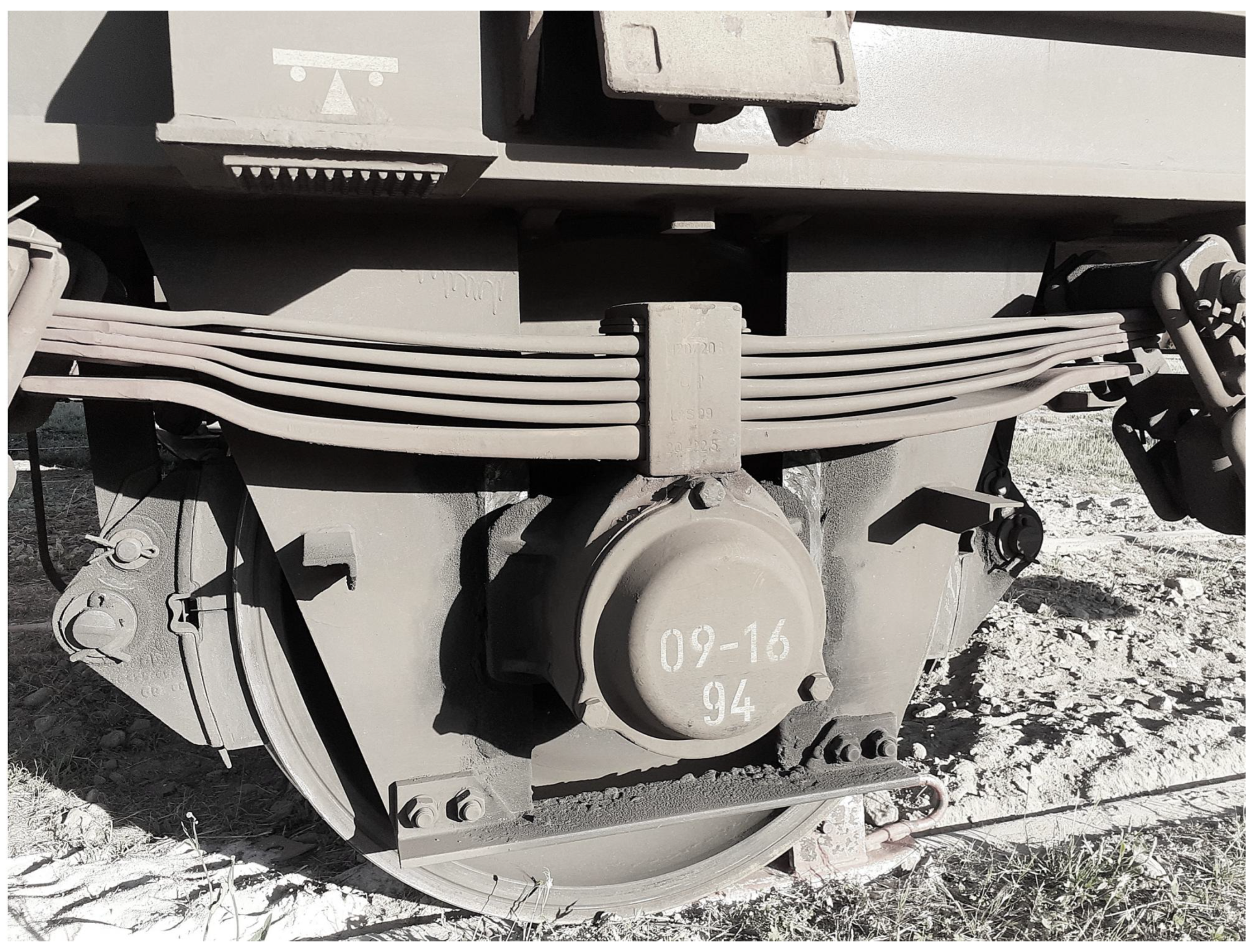
Figure 2.
Microstructure of the chromium-vanadium alloyed steel following the thermal treatments according ISO 683-14 standard [24].
Figure 2.
Microstructure of the chromium-vanadium alloyed steel following the thermal treatments according ISO 683-14 standard [24].
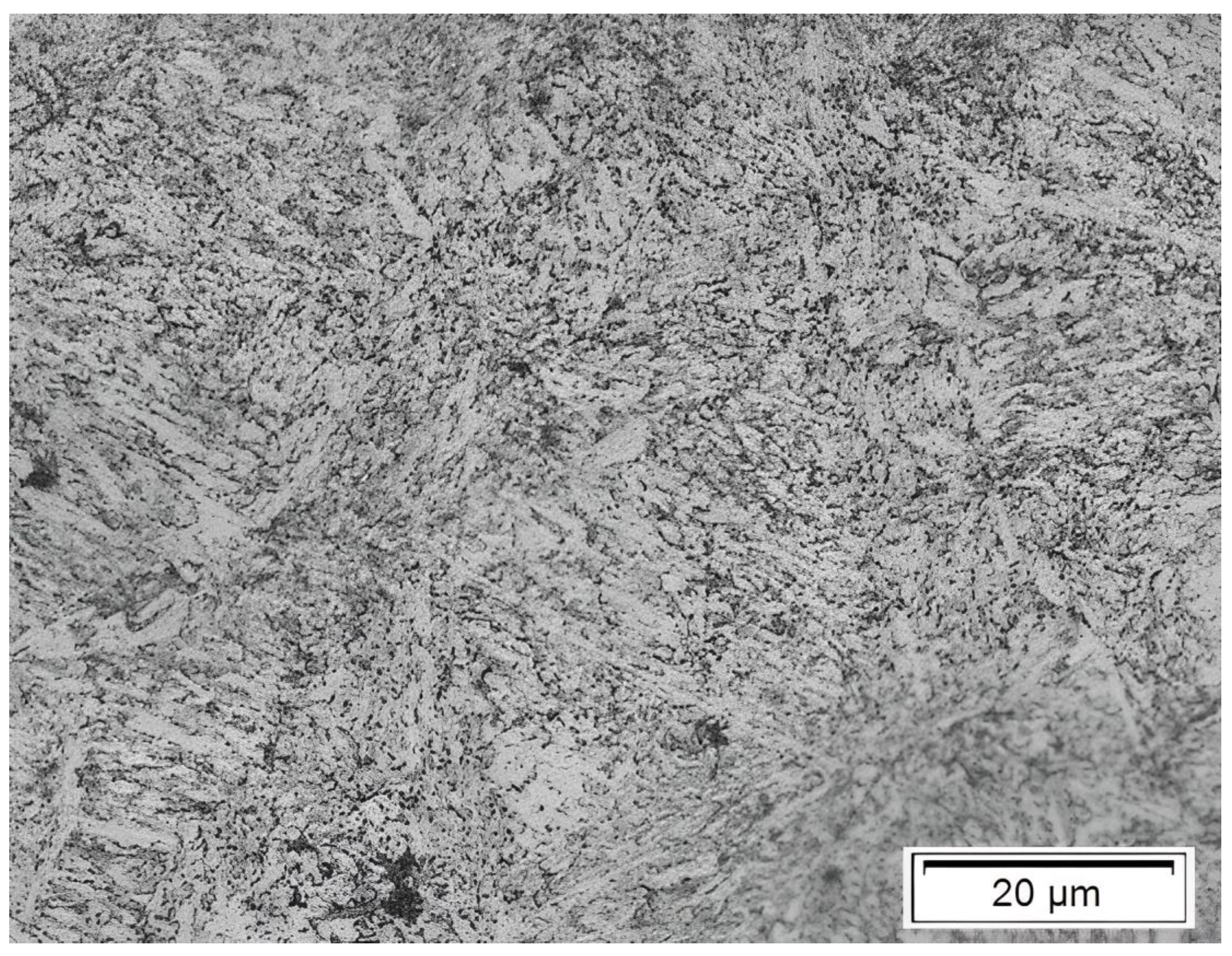
Figure 3.
Geometry of the specimens used in low-cycle fatigue tests, its geometric representation with identification of the geometrical parameters and the detail of the surface finishing (Dt. A1).
Figure 3.
Geometry of the specimens used in low-cycle fatigue tests, its geometric representation with identification of the geometrical parameters and the detail of the surface finishing (Dt. A1).
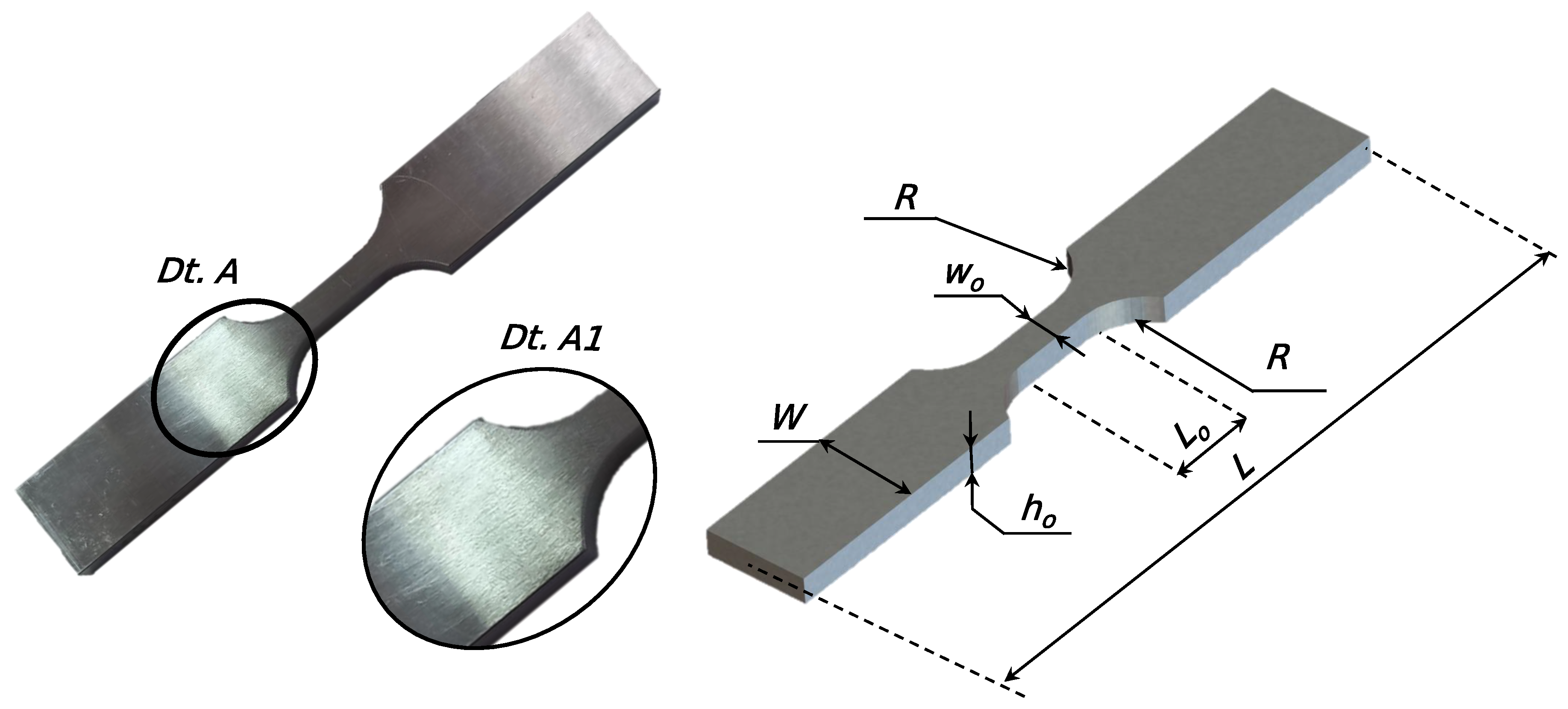
Figure 4.
Servo-hydraulic machine used for constant strain-controlled amplitude testing.
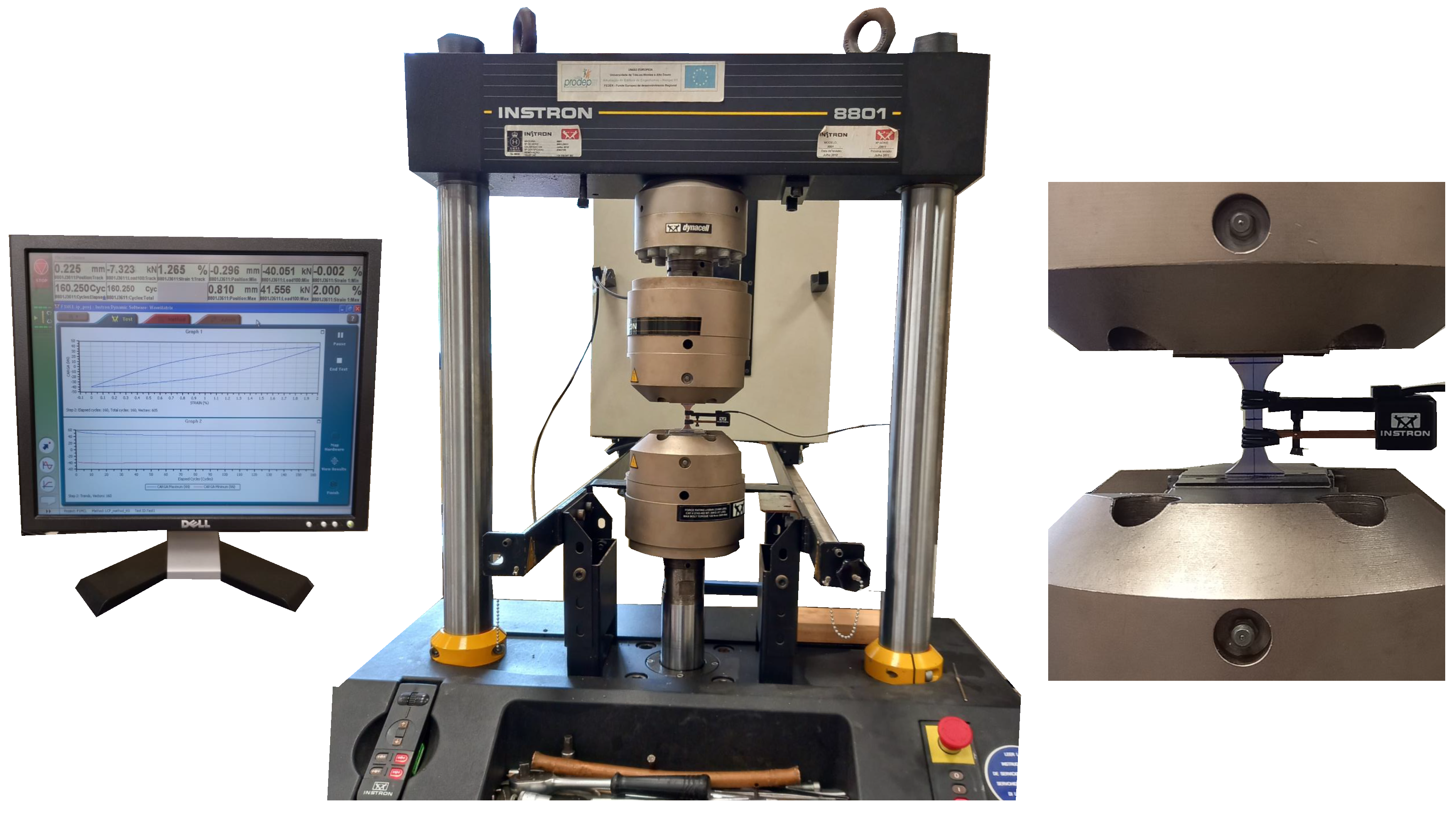
Figure 5.
Cyclic hysteresis curves for the 1st cycle and cycles corresponding to the 50% and 90% of total life.
Figure 5.
Cyclic hysteresis curves for the 1st cycle and cycles corresponding to the 50% and 90% of total life.
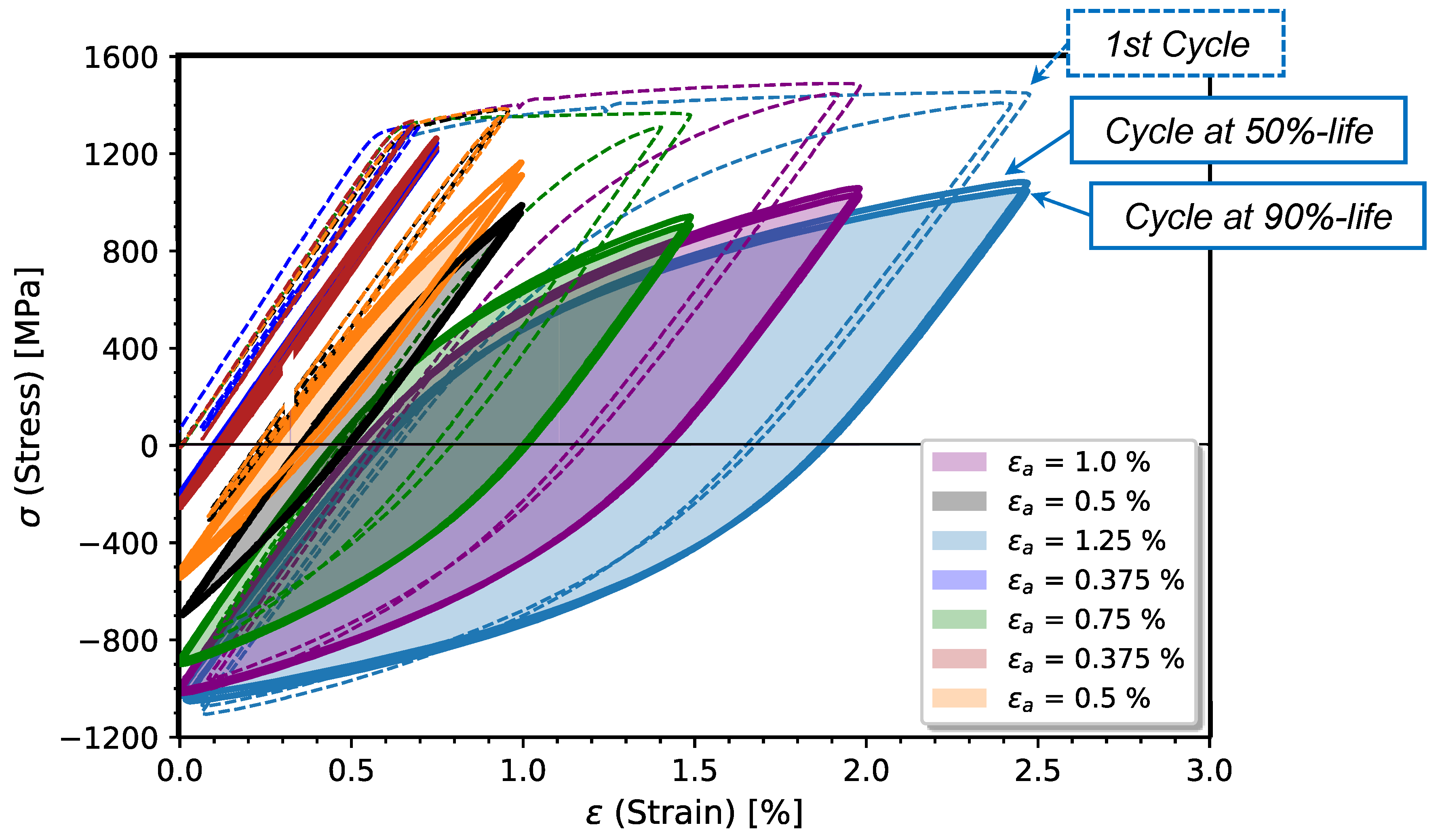
Figure 6.
Evolution and decomposition of the back stress components with the plastic strain amplitude.
Figure 6.
Evolution and decomposition of the back stress components with the plastic strain amplitude.
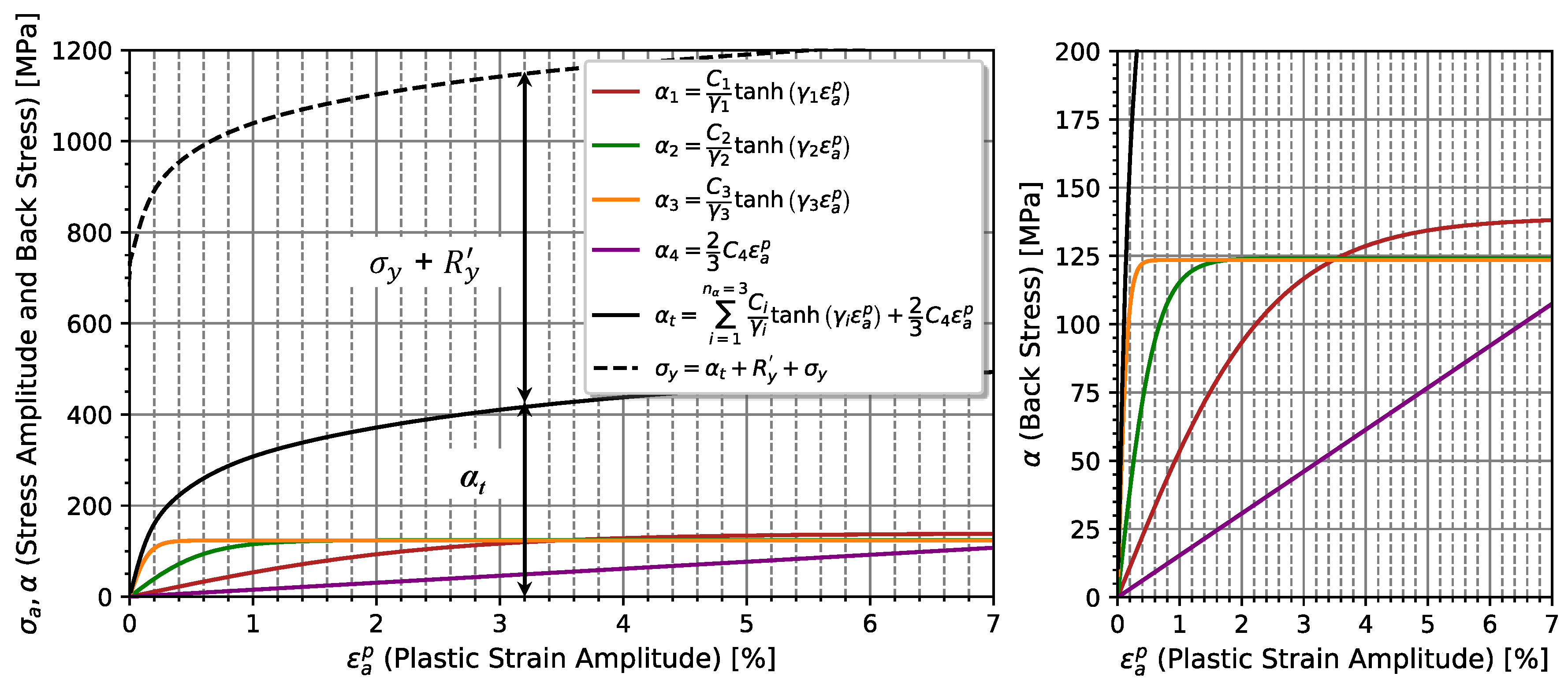
Figure 7.
Evolution of the amount of cyclic softening as function of the applied strain amplitude.
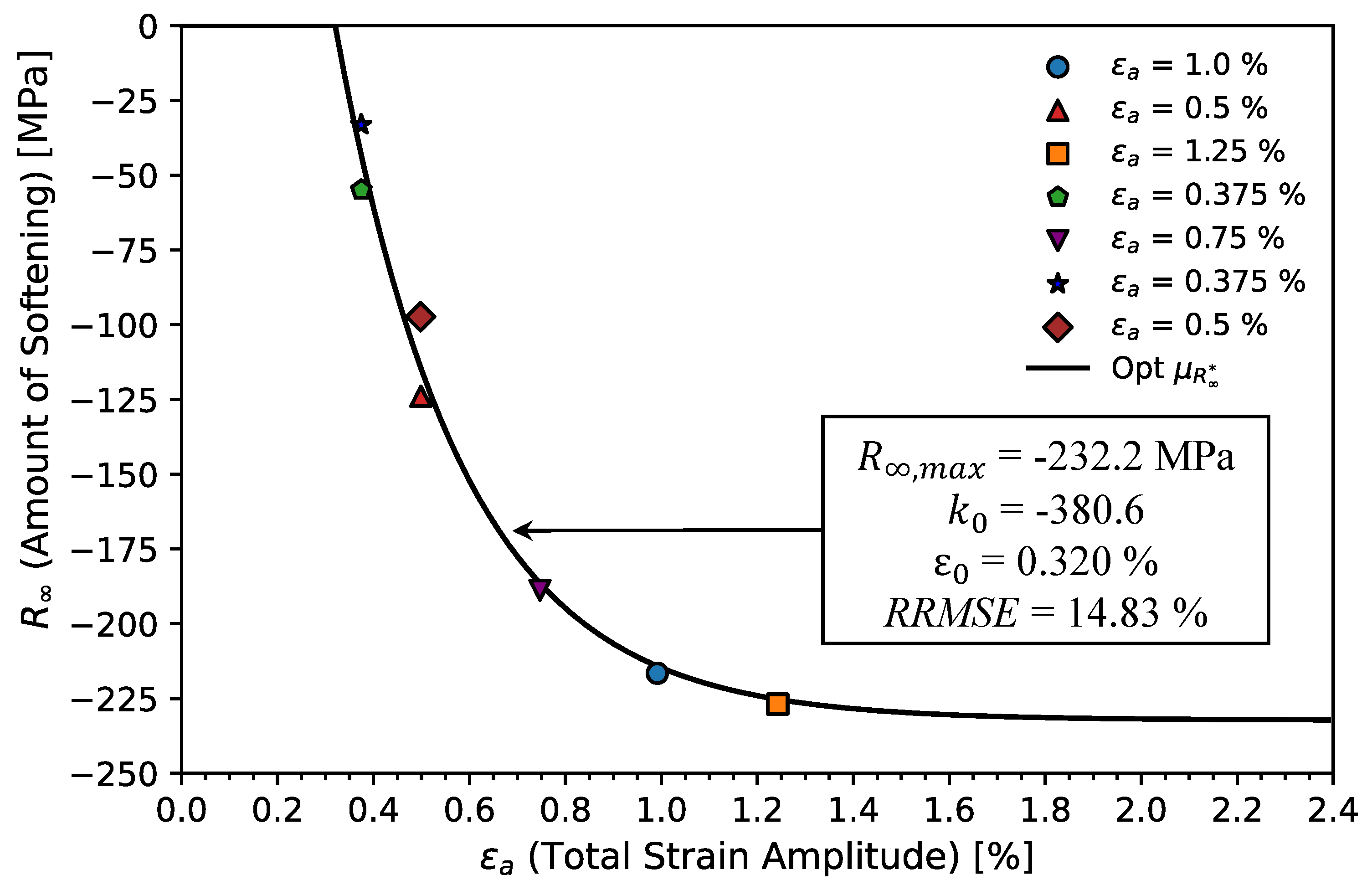
Figure 8.
Evolution of the normalized variation of the yield surface size evolution, throughout the cyclic testing until 90 % of the total life is reached.
Figure 8.
Evolution of the normalized variation of the yield surface size evolution, throughout the cyclic testing until 90 % of the total life is reached.
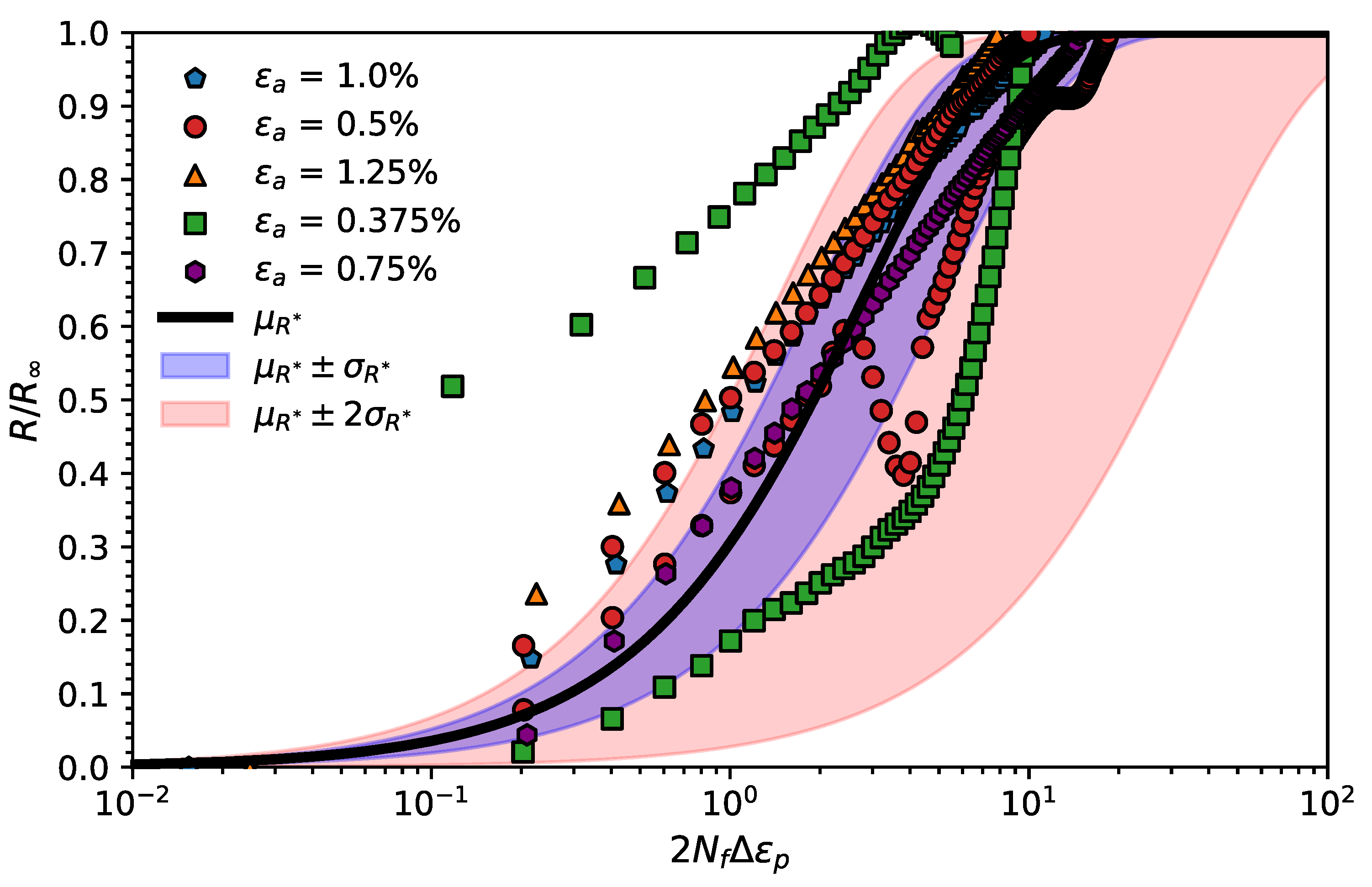
Figure 9.
Comparison between experimental data respectively for the first and the loop corresponding to 90 % of the total life with the simulation outcomes of the kinematic and isotropic hardening in terms of applied deformation (a) 0.75 %, (b) 1.00 %, (c) 1.25 %, and (d) 0.50 %. Note: The average parameter for (a), (b), and (c) is accordingly equation (12), and parameter for case (d) is determined for 0.50 %.
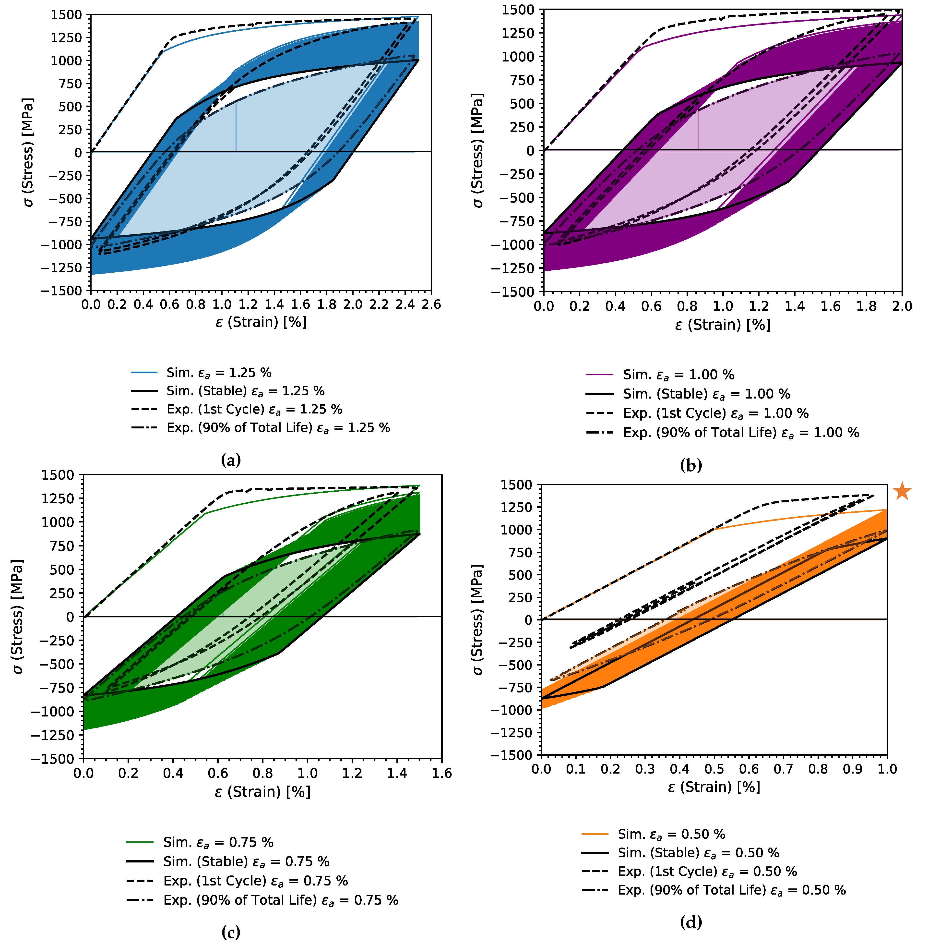
Figure 10.
Comparison of the variation of the maximum, minimum, and centre of the elastic surface limit between experimental data respectively for 90 % of the total life with the simulation outcomes of the kinematic and isotropic hardening in terms of applied deformation (a) 0.75 %, (b) 1.00 %, (c) 1.25 %, and (d) 0.50 %. Note: The average parameter for (a), (b), and (c) is accordingly equation (12), and parameter for case (d) is determined for 0.50 %.

Figure 11.
Error comparison between experimental data respectively for the first and the loop corresponding to 90 % of the total life with the simulation outcomes of the kinematic and isotropic hardening in terms of applied deformation (a) 0.75 %, (b) 1.00 %, (c) 1.25 %, and (d) 0.50 %. Note: The average parameter for (a), (b), and (c) is accordingly equation (12), and parameter for case (d) is determined for 0.50 %.
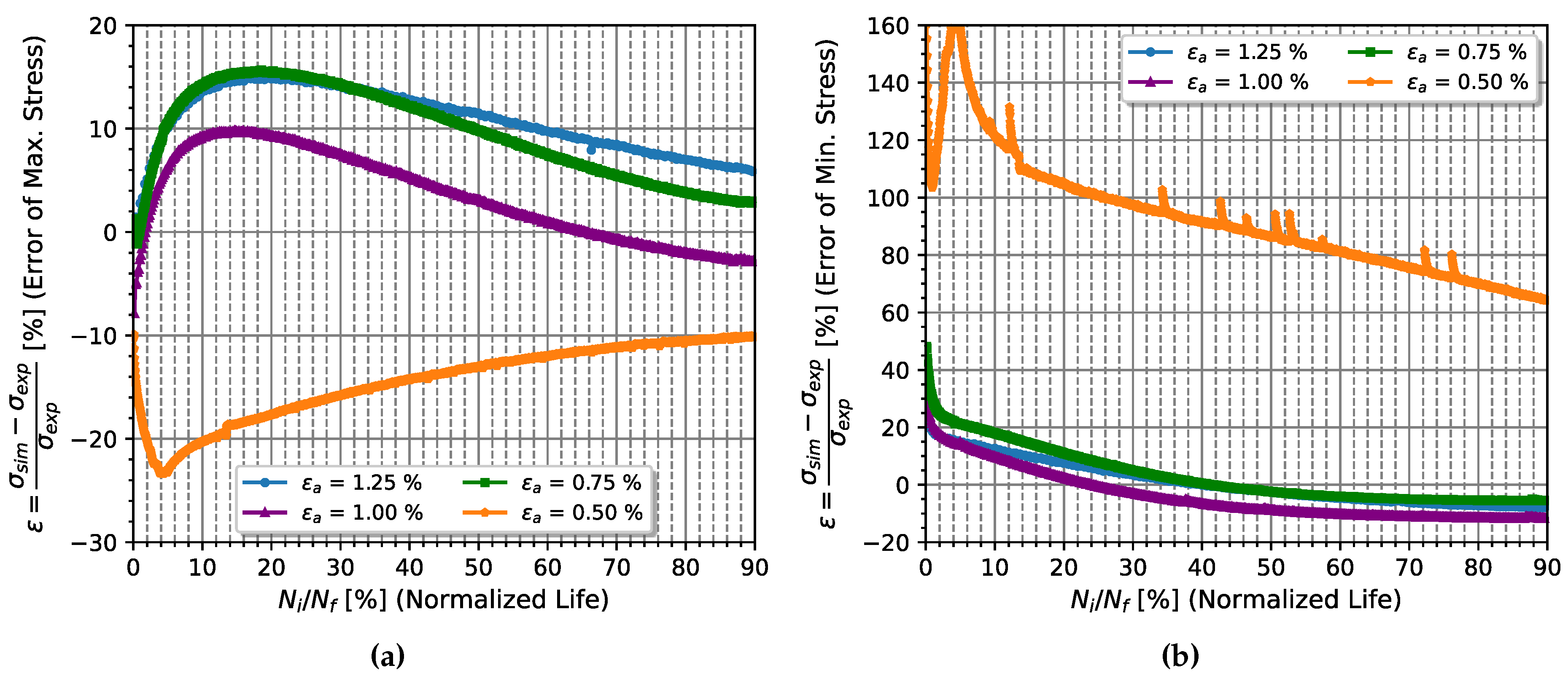
Table 2.
Monotonic mechanical properties obtained of the chromium-vanadium alloyed steel, 51CrV4 [24].
Table 2.
Monotonic mechanical properties obtained of the chromium-vanadium alloyed steel, 51CrV4 [24].
| E | |||||
|---|---|---|---|---|---|
| [GPa] | [MPa] | [MPa] | [%] | [%] | |
| Average | 7.53 | 34.69 | |||
| Std. Dev. [24] | |||||
| DIN 51CrV4 (1.8159) | 200 | 1200 | 1350-1650 | 6 | 30 |
Table 3.
Geometry statistics of low-cycle fatigue specimen and general testing parameters.
| L | W | R | d/dt | |||||
|---|---|---|---|---|---|---|---|---|
| [mm] | [mm] | [mm] | [mm] | [mm] | [mm] | [%/s] | ||
| 15 | 135 | 20 | 12 | 0.0 | 0.8 | |||
Table 4.
Hardening parameters that define the Chaboche’s kinematic hardening model for steady-state cyclic conditions at 50 and 90 % of the total life to failure.
Table 4.
Hardening parameters that define the Chaboche’s kinematic hardening model for steady-state cyclic conditions at 50 and 90 % of the total life to failure.
| RRMSE * | ||||||||||||
|---|---|---|---|---|---|---|---|---|---|---|---|---|
| [MPa] | [ MPa] | [ MPa] | [MPa] | [MPa] | [MPa] | [MPa] | % | |||||
| 50% | 731.5 | -357.7 | 1514.3 | 0.0790 | 80097.1 | 648.4 | 20486.2 | 164.9 | 5650.1 | 40.64 | 2302.7 | 0.2594 |
| 90% | 676.7 | -412.5 | 1576.5 | 0.0918 | 81701.2 | 610.2 | 22035.4 | 159.1 | 6332.2 | 39.93 | 2673.4 | 0.2853 |
| Diff. | 7.49 | 15.32 | 4.09 | 16.20 | 2.00 | 5.89 | 7.56 | 3.49 | 12.07 | 1.75 | 13.87 | 9.98 |
*RRMSE is the relative root mean square error.
Table 5.
Elasto-plastic parameters that define the Hooke, Voce, and Chaboche hardening models for steady-state cyclic conditions at 90 % of the total life to failure.
Table 5.
Elasto-plastic parameters that define the Hooke, Voce, and Chaboche hardening models for steady-state cyclic conditions at 90 % of the total life to failure.
| E | ||||||||||||
|---|---|---|---|---|---|---|---|---|---|---|---|---|
| [GPa] | [MPa] | [MPa] | [MPa] | [MPa] | [MPa] | [MPa] | [MPa] | |||||
| 202.5 | 0.29 | 1089.2 | -232.2 | 0.3705 | 676.7 | 80097.1 | 648.4 | 20486.2 | 164.9 | 5650.1 | 40.64 | 2302.7 |
Disclaimer/Publisher’s Note: The statements, opinions and data contained in all publications are solely those of the individual author(s) and contributor(s) and not of MDPI and/or the editor(s). MDPI and/or the editor(s) disclaim responsibility for any injury to people or property resulting from any ideas, methods, instructions or products referred to in the content. |
© 2025 by the authors. Licensee MDPI, Basel, Switzerland. This article is an open access article distributed under the terms and conditions of the Creative Commons Attribution (CC BY) license (http://creativecommons.org/licenses/by/4.0/).
Copyright: This open access article is published under a Creative Commons CC BY 4.0 license, which permit the free download, distribution, and reuse, provided that the author and preprint are cited in any reuse.


