
Submitted:
21 January 2025
Posted:
23 January 2025
You are already at the latest version
Abstract
Molecular dynamics Molecular dynamics (MD) simulations have proven useful in studying the dynamics of Biomolecules, for instance proteins. However, the computational cost for conducting such simulations is high as reflected in the number of core-hours consumed in high performance computing (HPC) clusters. Although some techniques are available for enhancing the sampling of the conformational space, they usually make assumptions about the system by introducing empirical parameters. Machine learning (ML) models can overcome this issue because here, important features of the landscape can be inferred from the data themselves. In this work, we use an autoencoder ML model with three different flavors: Variational, Wasserstein, and Denoising to generate new protein conformations using MD trajectories as the training data. These generated structures can potentially enhance the ensemble of the original MD data.
Keywords:
molecular
; dynamics
; autoencoders
; proteins
1. Introduction
Molecular dynamics (MD) simulations have proven useful to study the dynamics of Biomolecules, for instance proteins. However, these simulations are computationally expensive and consume many core-hours of high performance computing (HPC) clusters to achieve enough sampling of the energy landscape. To enhance the sampled configurational space, several techniques have been used in the past but some of them make assumptions on the system for instance using predefined collective variables [1,2,3] or by modifications of the energy landscape [4] where empirical parameters are introduced.
More recently, machine learning (ML) models are being used to extract relevant features from the energy landscape which are then used to infer/interpolate new data. In particular, in the autoencoder (AE) machine learning model, one performs the training by first reducing the dimensionality of the data gradually to build a latent space and then use the compressed latent space to reconstruct the initial data through some metrics and regularization terms [5,6]. One advantage of the AE models is the reduced number of training parameters that are involved w.r.t. the fully connected neural networks. Once trained, these models can be used to generate new data. In the context of proteins, one can use existing data sets of protein structures collected through computational methods, classical (MD) or quantum mechanical (DFT, HF, among others) as the training data sets. These trained models can be used to extend the sampled ensemble of protein conformations using cheaper computational resources. In addition to the computational data sets, ML models open the window to include data from experiments, such as NMR, Cryo-EM, and X-ray crystallography.
In the present work, we used three different flavors of AE models to generate new protein conformations using MD trajectories of the Shikimate Kinase enzyme for the training data set. A key difference between these three models is the way in which the latent space is created. For the first AE model, we used the variational autoencoder (VAE) model of Zhu et al. [7] which was originally used to extend the sampled space of intrinsic disordered proteins (IDPs). In the second and third models, we studied the Wasserstein autoencoder (WAE) [8,9], and the Denoising autoencoder (DAE) [10] models, respectively. Details about the three models can be found in the Materials and Methods section. Because AE models are used as components of more complex workflows, understanding their performance can be beneficial when they are employed in standalone or as part of a larger workflow. The results of the three models are compared using standard analysis tools for MD.
2. Materials and Methods
2.1. Data Collection
The MD trajectory used in the present study was taken initially from [11], where the Shikimate Kinase (SK) enzyme was simulated in the absence of substrates, and further extended to achieve 5 μs. SK has three main domains called SB, β, and LID domains which are highly flexible and allow this enzyme to harbor substrates for catalysis. Details for the MD simulations can be found in this reference paper. Frames for data collection were saved every 0.05 ns resulting in 1 frames.
2.2. Methods
A schematic view of the three AE models is presented in Figure 1 (a)-(c), VAE, WAE, and DAE, respectively.
2.2.1. Variational Autoencoder (VAE) Model
In the VAE model, the encoder network is modeled through the distribution that maps the input space (ℵ) to the latent space (Ƶ). The decoder or generative model is given by the distribution. The loss function is computed as in Ref. [7]:
is the reconstruction loss computed as the logarithmic mean squared error between the input data and the reconstructed data. is the Kullback-Leibler (KL) [12] divergence regularization term.
2.2.2. Wasserstein Autoencoder (WAE) Model
The WAE model uses a marginal distribution of the encoder distribution . In this model the loss is given by,
Here, the reconstruction error was computed as the mean squared error between the input and reconstructed data. The maximum mean discrepancy (MMD) [13,14] loss between two probability distributions and , in the present case the Gaussian prior and latent space marginal () distributions, was computed as follows:
where the kernel function is the radial basis function (RBF) defined by,
with a standard deviation . The parameter is a weighting factor for the MMD term which has a value of 10 in the present simulations.
2.2.3. Denoising Autoencoder (DAE) Model
In this model, the initial data are corrupted with Gaussian noise. The idea of adding/subtracting noise from input data has been used in other ML models [15,16]. The loss function is computed in DAE by considering only the reconstruction error:
This error is calculated as the mean squared error between the input and reconstructed data.
2.3. Postprocessing and Analysis of Data
The MD trajectories were postprocessed with the Visual Molecular Dynamics (VMD) [17] (v. 1.9.4) software by extracting all atoms in the protein structure except for the hydrogen atoms. The data set for the autoencoder models was partitioned in 80% for the training set (TrS) and 20% for the testing set (TsS) using the preprocessing script given in Ref. [7]. Models’ training was done with Keras (v. 2.11) and Tensorflow (v. 2.11) libraries. To collect the performance metrics for the models (Table 1) we used 5 epochs as simulations displayed convergence already for this value.
The integrity of reconstructed structures from the three AE methods was analyzed through the Spearman correlation coefficient (SpCC) which measures the correlation in the monotonic growing between the ranked distributions for the original and reconstructed data. For instance, a SpCC value close to +1 indicates that both distributions grow in the same direction for each data sample. In addition to this, we also used the mean square error (MSE) between these two distributions.
The conformations generated (a total of 1) were inspected with standard analysis tools for MD trajectories including the root mean square deviation (RMSD), root mean square fluctuation (RMSF), and principal component analysis (PCA). For the RMSD calculations, the reference structure was the first frame of the MD trajectory in all cases and the backbone atoms were selected for the computation. In the case of the RMSF results, only the Cα atoms were selected. The RMSF curves for the AE models were translated to match the value of the MD RMSF at 5 Å. Regarding PCA, all protein atoms except for hydrogen atoms were considered for the computation.
2.4. Code Availability
The codes for the three autoencoder models can be found here https://github.com/pojeda/AE-variants.
3. Results and Discussion
The SpCC for the SK protein showed values for both the training and testing sets larger than those reported in Ref. [7]. This can be due to the fact that SK has a more ordered structure in comparison to the IDPs discussed in that reference. The values for SpCC were close for the three different methods for this SK protein ~0.99. Regarding, the MSE values were similar for all methods in the training set, but we noticed that DAE had a lower value for the testing set w.r.t. to the other two methods. Notice that we have not conducted an extensive exploration of the hyperparameters involved in the model and we used values similar to those of Zhu et al. [7]. Results for SpCC and MSE can be seen in Table 1.
We noticed that even though the SpCC and MSE values showed that the reconstructed data was close to the original data, the generated protein structures presented distortions in the bond lengths especially in the flexible LID region. This issue has been previously faced by postprocessing the structures [7,18]. Other approaches can be used, for instance graph neural networks [19] and rigid body transformations [20].
By using the trained models, new conformations were generated. We investigated the capability of the models to generate an ensemble of conformations similar to the original MD ensemble. Thus, as a first approach we took the initial structure from the MD simulations and computed the RMSD values for the models. This can give us an idea of how the conformational space was explored. Using the RMSD values we constructed histograms of counts as it can be seen in Figure 2. The distribution for the MD case showed a peak ~2.4 Å while the AE models had a peak ~2.25 Å. The exploration range for the AE models was limited, especially for the DAE model where generated structures were close to the peak value. In all models, structures with RMSD values lower than 1.4 Å and close the initial one were not generated.
The variations in the displacement of the protein residues can be monitored through the RMSF values which are presented in Figure 3. Because the RMSF values can be correlated to the temperature of the environment, especially for the highly flexible regions, we argue that the three different AE models display a lower temperature than the MD data. However, the trend of the fluctuations follows a similar pattern as in the MD case for the flexible SB, β, and LID domains. Fluctuations are considerably reduced in the DAE model.
We also monitored the sampling of the conformational space for the generated structures in a reduced dimensional space through principal component analysis (PCA), see Figure 4. Here, we can see that the VAE model learns some structure from dynamical data which is reflected in the pattern displayed by the corresponding plot.
The PCA plots show that the different AE models can help to sample the conformational space in different ways. In the case of WAE the points corresponding to the generated structures are spread in the projected space while in DAE model the data points are more localized.
4. Conclusions
We have compared three different flavors of AE models, i.e. Variational, Wasserstein, and Denoising to generate protein structures not included in the original data from MD simulations. According to the RMSD and PCA analysis, the three models explore the conformational space in a different way, for instance the WAE model showed spread distribution of structures while the DAE displayed a more restricted distribution.
The RMSF analysis suggests that the generated conformations, considered as an ensemble, are not at the same temperature as the original MD ensemble. In particular, the flexible regions displayed attenuated fluctuations w.r.t. to the original MD data.
One shortcoming of the present simulations is that the bond lengths and angles of the generated structures are distorted, which opens the possibility for further improvement of the models.
Acknowledgments
This research was conducted using the resources of High Performance Computing Center North (HPC2N).
References
- Laio, A.; Parrinello, M. Escaping Free-Energy Minima. PNAS 2002, 99, 12562–12566. [Google Scholar] [CrossRef] [PubMed]
- Bussi, G.; Laio, A.; Parrinello, M. Equilibrium Free Energies from Nonequilibrium Metadynamics. Phys. Rev. Lett. 2006, 96, 090601. [Google Scholar] [CrossRef] [PubMed]
- Kim, J.; Straub, J.E.; Keyes, T. Statistical-Temperature Monte Carlo and Molecular Dynamics Algorithms. Phys. Rev. Lett. 2006, 97, 050601. [Google Scholar] [CrossRef] [PubMed]
- Pang, Y.T.; Miao, Y.; Wang, Y.; McCammon, J.A. Gaussian Accelerated Molecular Dynamics in NAMD. J. Chem. Theory Comput. 2017, 13, 9–19. [Google Scholar] [CrossRef] [PubMed]
- Bourlard, H.; Kamp, Y. Auto-Association by Multilayer Perceptrons and Singular Value Decomposition. Biol. Cybern. 1988, 59, 291–294. [Google Scholar] [CrossRef] [PubMed]
- Hinton, G.E.; Salakhutdinov, R.R. Reducing the Dimensionality of Data with Neural Networks. Science 2006, 313, 504–507. [Google Scholar] [CrossRef] [PubMed]
- Zhu, J.-J.; Zhang, N.-J.; Wei, T.; Chen, H.-F. Enhancing Conformational Sampling for Intrinsically Disordered and Ordered Proteins by Variational Autoencoder. International Journal of Molecular Sciences 2023, 24, 6896. [Google Scholar] [CrossRef] [PubMed]
- Bousquet, O.; Gelly, S.; Tolstikhin, I.; Simon-Gabriel, C.-J.; Schoelkopf, B. From Optimal Transport to Generative Modeling: The VEGAN Cookbook 2017.
- Tolstikhin, I.; Bousquet, O.; Gelly, S.; Schoelkopf, B. Wasserstein Auto-Encoders 2019.
- Vincent, P.; Larochelle, H.; Bengio, Y.; Manzagol, P.-A. Extracting and Composing Robust Features with Denoising Autoencoders. In Proceedings of the Proceedings of the 25th international conference on Machine learning - ICML ’08; ACM Press: Helsinki, Finland, 2008; pp. 1096–1103. [Google Scholar]
- Ojeda-May, P. Exploring the Dynamics of Shikimate Kinase through Molecular Mechanics. Biophysica 2022, 2, 194–202. [Google Scholar] [CrossRef]
- Kullback, S.; Leibler, R.A. On Information and Sufficiency. Ann. Math. Statist. 1951, 22, 79–86. [Google Scholar] [CrossRef]
- Gretton, A.; Borgwardt, K.M.; Rasch, M.J.; Schölkopf, B.; Smola, A. A Kernel Two-Sample Test. Journal of Machine Learning Research 2012, 13, 723–773. [Google Scholar]
- Vayer, T.; Gribonval, R. Controlling Wasserstein Distances by Kernel Norms with Application to Compressive Statistical Learning. Journal of Machine Learning Research 2023, 24, 1–51. [Google Scholar]
- Anand, N.; Achim, T. Protein Structure and Sequence Generation with Equivariant Denoising Diffusion Probabilistic Models 2022.
- Watson, J.L.; Juergens, D.; Bennett, N.R.; Trippe, B.L.; Yim, J.; Eisenach, H.E.; Ahern, W.; Borst, A.J.; Ragotte, R.J.; Milles, L.F.; et al. De Novo Design of Protein Structure and Function with RFdiffusion. Nature 2023, 620, 1089–1100. [Google Scholar] [CrossRef] [PubMed]
- Humphrey, W.; Dalke, A.; Schulten, K. VMD: Visual Molecular Dynamics. Journal of Molecular Graphics 1996, 14, 33–38. [Google Scholar] [CrossRef] [PubMed]
- Jin, Y.; Johannissen, L.O.; Hay, S. Predicting New Protein Conformations from Molecular Dynamics Simulation Conformational Landscapes and Machine Learning. Proteins: Structure, Function, and Bioinformatics 2021, 89, 915–921. [Google Scholar] [CrossRef] [PubMed]
- Zhu, J.; Li, Z.; Tong, H.; Lu, Z.; Zhang, N.; Wei, T.; Chen, H.-F. Phanto-IDP: Compact Model for Precise Intrinsically Disordered Protein Backbone Generation and Enhanced Sampling. Briefings in Bioinformatics 2024, 25. [Google Scholar] [CrossRef] [PubMed]
- Yim, J.; Trippe, B.L.; Bortoli, V.D.; Mathieu, E.; Doucet, A.; Barzilay, R.; Jaakkola, T. SE(3) Diffusion Model with Application to Protein Backbone Generation 2023.
Figure 1.
Schematic view of how the three models VAE, WAE, and DAE map/build the input (ℵ) and latent spaces (Ƶ). (a) In VAE, the encoder network is forced to match individual data samples to the prior distribution.; (b) WAE uses the marginal of over input samples to match a collective prior. is the latent variable generative model. (c) In DAE, the initial data samples are corrupted with noise, and these data are used to build the latent space.
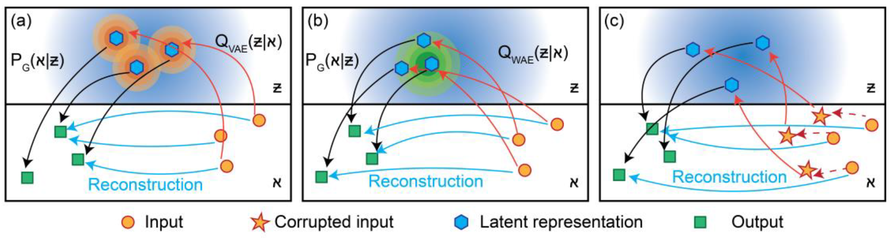
Figure 2.
Histograms of counts for the RMSD values computed for the MD data (a), and the VAE (b), WAE (c), and DAE (d) models.
Figure 2.
Histograms of counts for the RMSD values computed for the MD data (a), and the VAE (b), WAE (c), and DAE (d) models.
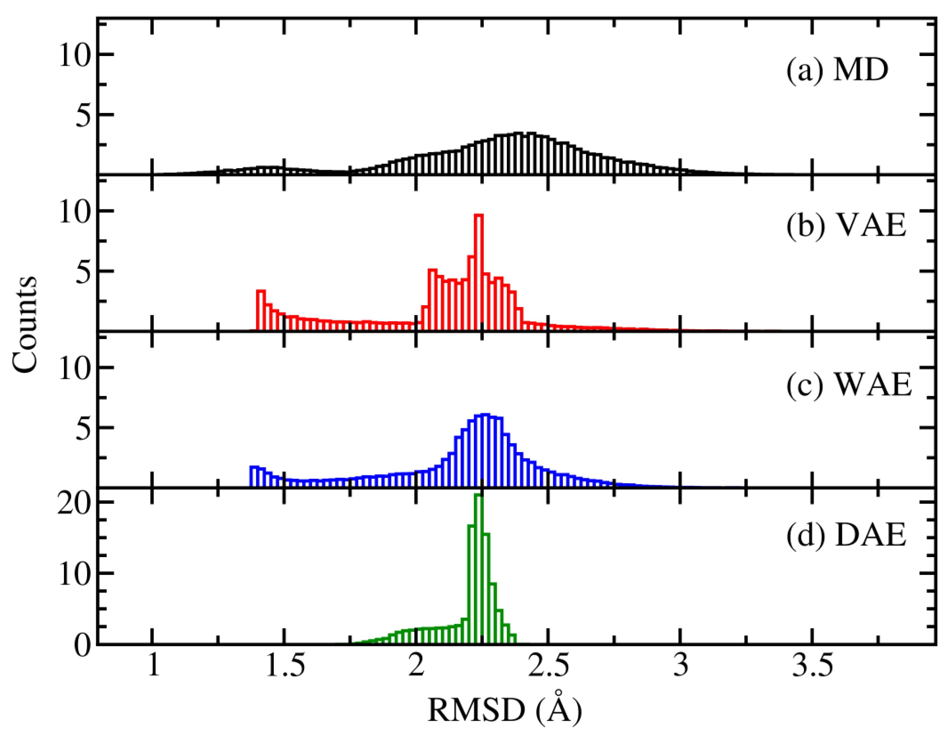
Figure 3.
RMSFs computed for the MD, and the three AE models. Overall, the fluctuations were reduced in the flexible parts of the protein structure especially in the DAE model.
Figure 3.
RMSFs computed for the MD, and the three AE models. Overall, the fluctuations were reduced in the flexible parts of the protein structure especially in the DAE model.
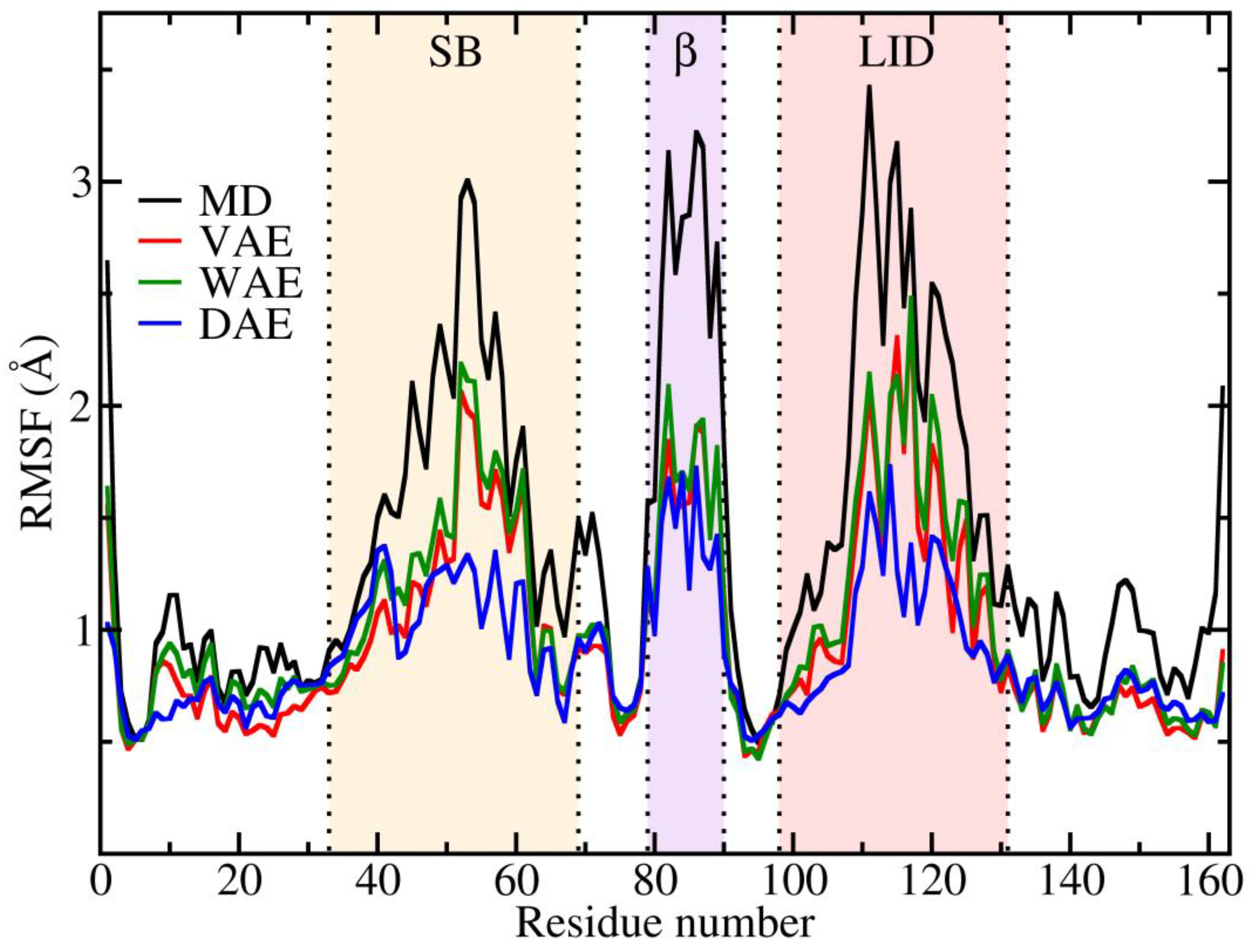
Figure 4.
(a) Projected MD trajectory of SK protein onto the first two eigenvectors. (b)-(d) Projected protein structures generated with the three AE models: VAE, WAE, and DAE, respectively, onto the first two eigenvectors from the MD trajectory.
Figure 4.
(a) Projected MD trajectory of SK protein onto the first two eigenvectors. (b)-(d) Projected protein structures generated with the three AE models: VAE, WAE, and DAE, respectively, onto the first two eigenvectors from the MD trajectory.
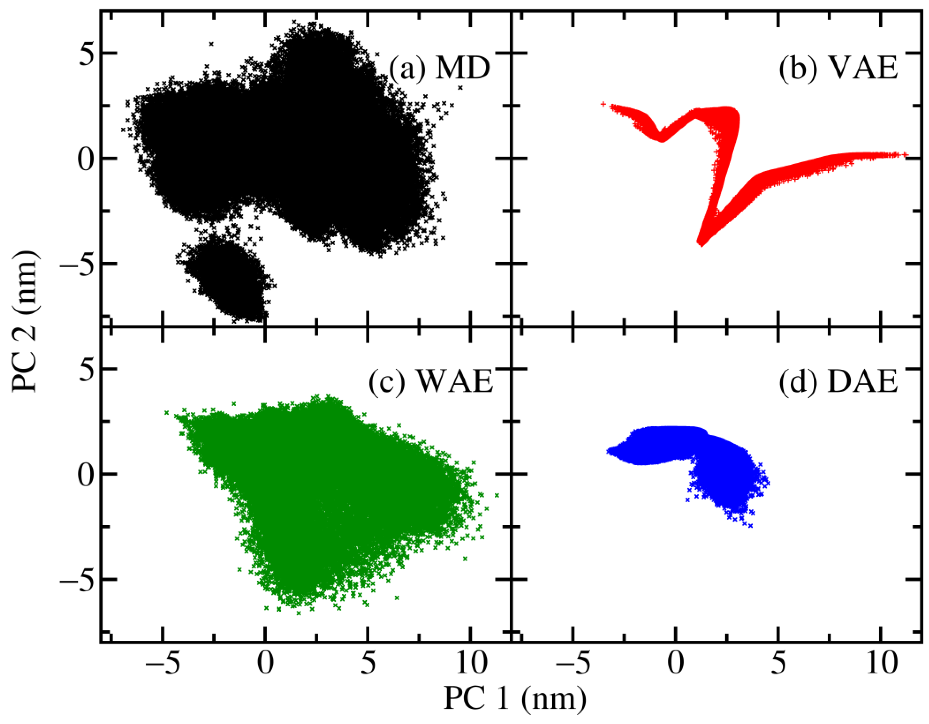

Table 1.
SpCC and MSE values for the VAE, WAE, and DAE models using the TrS and TsS.
| Model | SpCC TrS | SpCC TsS | MSE TrS (Å2) | MSE TsS (Å2) |
|---|---|---|---|---|
| VAE | 0.997 | 0.992 | 0.64 | 1.60 |
| WAE | 0.996 | 0.992 | 0.69 | 1.59 |
| DAE | 0.996 | 0.993 | 0.66 | 1.49 |
Disclaimer/Publisher’s Note: The statements, opinions and data contained in all publications are solely those of the individual author(s) and contributor(s) and not of MDPI and/or the editor(s). MDPI and/or the editor(s) disclaim responsibility for any injury to people or property resulting from any ideas, methods, instructions or products referred to in the content. |
© 2025 by the authors. Licensee MDPI, Basel, Switzerland. This article is an open access article distributed under the terms and conditions of the Creative Commons Attribution (CC BY) license (http://creativecommons.org/licenses/by/4.0/).
Copyright: This open access article is published under a Creative Commons CC BY 4.0 license, which permit the free download, distribution, and reuse, provided that the author and preprint are cited in any reuse.


