Submitted:
22 January 2025
Posted:
22 January 2025
You are already at the latest version
Abstract
Federated Learning represents a newly emerging methodology in the field of machine learning, it enables distributed agents to collaboratively learn a centralized model without sharing their raw data. Some scholars have already proposed many first-order algorithms and second-order algorithms for federated learning to reduce communication costs and speed up convergence. However, these algorithms generally rely on gradient or Hessian information, and we find it difficult to solve such federated optimization problems when the analytical expression of the loss function is not available, that is, when gradient information is not available. Therefore, we employed derivative-free federated zeroth-order optimization in this paper which not rely on specific gradient information, but instead utilizes the changes in function values or model outputs to estimate the optimization direction. Furthermore, to enhance the performance of derivative-free zeroth-order optimization, we propose an effective adaptive algorithm that can dynamically adjust the learning rate and other hyperparameters based on the performance during the optimization process, aiming to accelerate convergence. We rigorously analyze the convergence of our approach, and the experimental findings demonstrate our method indeed can achieve faster convergence speed on the MNIST and CIFAR-10 datasets in cases where gradient information is not available.
Keywords:
Federated Learning
; Zero-Order optimization
; Adaptive
; convergence
1. Introduction
With the rapid development of big data and artificial intelligence technologies, machine learning has become one of the key technologies in various fields. However, in practical applications, issues of data privacy and security have become a non-negligible challenge. In traditional machine learning, data usually needs to be sent to data centers for model training, but in the process of transmission, it faces the problems of data leakage and privacy protection. To address this issue, federated learning(FL) [1], an emerging distributed machine learning technology, has emerged. It achieves collaborative learning among multiple data sources, and while protecting data privacy by exchanging model parameters instead of raw data. Currently, FL is utilized across diverse domains such as autonomous driving [2], personalized recommendation systems [3], and medical informatics [4], among others.
However, existing federated learning methods also have some obvious shortcomings. For instance, some federated learning methods are unable to effectively prevent privacy leaks when faced with complex attack techniques, and the convergence speed of current federated learning algorithms remains a bottleneck. Additionally, designing more efficient optimization algorithms tailored to different types of models and tasks is also an urgent issue that needs to be addressed. Researching how to enhance the privacy protection capabilities of federated learning is of great significance in an environment where data security and privacy protection are increasingly critical. This not only safeguards users’ personal information but also promotes the widespread application of federated learning technology across various domains. In practical applications, federated learning needs to meet the demands of various scenarios. By investigating the issue of slow convergence speed, it can better satisfy these practical application needs and enhance the practicality and value of federated learning.
In recent years, the federated optimization for model training has increasingly captured the interest of both academic researchers and industry professionals. To achieve fast convergence rates and reduce communication loads, a wide range of algorithms have been proposed, including first-order methods (such as FedAvg [1], FedFOR [5], FedFomo [6]) and second-order methods (such as Fed-Sophia [7]). Most of these algorithms rely on gradient or Hessian information, and these methods are often only applicable to differentiable functions. However, when the objective function is difficult to compute gradients or the gradient computation cost is excessively high, these algorithms will not be able to solve such problems, such as in the case of black-box functions and in federated hyperparameter tuning [8], so we must look for other solutions. To alleviate the reliance on gradient or Hessian information, the federated zeroth-order optimization (FedZO) algorithm is proposed in [9] through the integration of zeroth-order optimization into the federated learning. The characteristic of derivative-free zeroth-order optimization is that it only queries the objective function values to tackle the problems of federated optimization. It approximates the full gradient and stochastic gradient of the function using function values, without using gradient and Hessian information. In each round of communication, several local updates are performed utilizes a two-point stochastic gradient estimator. Some recent studies such as [10] and [11] have also employed the zeroth-order idea. [10] proposed FedDisco algorithm, leveraging zeroth-order optimization techniques reduces communication overhead significantly. [11] designed a federated zeroth-order algorithm FedZeN, it focused on convex optimization and estimate the curvature of the global objective.
However, existing zeroth-order methods rely solely on function value information, lacking the utilization of gradient and other relevant information. So in complex federated learning scenarios, this method may result in the model failing to fully leverage the feature information of the data, leading to the need for more iterations to achieve convergence during the optimization process. This significantly increases computational time and affects model performance and convergence speed. If the convergence speed of zeroth-order optimization can be accelerated, it can play a better role in scenarios with limited resources such as large-scale distributed optimization and edge computing, improving resource utilization efficiency and thereby promoting the widespread deployment of optimization technologies in resource-sensitive applications.
The emergence of adaptive methods has effectively alleviated the problem of slow convergence. In deep learning, an excessively large learning rate may lead to unstable model training, resulting in overfitting or underfitting. Besides, traditional fixed learning rate methods often struggle to adapt to complex and diverse training data and model structures, potentially leading to slow convergence speed of the model. The adaptive method can dynamically adjust the learning rate based on feedback from the training process, thereby accelerating the convergence of the model. In addition, compared with stochastic gradient descent, this method can also escape saddle points more quickly [12]. Therefore, introducing it in practice represents a crucial approach to enhancing the performance of federated learning algorithms.
However, improper design of adaptive federated learning methods may lead to convergence issues [13]. Reddi et al. [14] first proposed a federated version of the adaptive optimizer, among them are FedAdagrad and FedYogi. However, their analysis is only valid under the condition that (where is the decay parameter), which cannot leverage the advantages of momentum. In the algorithm FedCAMS [15], it provides a complete proof, but it does not improve the convergence speed. Moreover, they usually require a global learning rate for initialization and adjustment, and the selection of this global learning rate may affect the performance of the algorithm. Existing adaptive methods still have shortcomings such as lagging response to complex environmental changes and high consumption of computational resources. Our goal is to design adaptive algorithms tailored to various real-world scenarios, characterized by efficiency, precision, and flexibility, so as to rapidly adapt to environmental changes, optimize resource allocation, and provide robust support for development across various fields.
Based on the above, we combine the gradient-free optimization with adaptive methods, aiming to leverage the advantages of both to solve the problem of unavailable gradient information of the objective function in a finite-sum optimization problem, while achieving fast convergence and effectively improving the training efficiency and performance of the model.
Contributions The contributions of this paper are summarized as follows:
- By combining the zero-order optimization and adaptive gradient method, we have proposed a novel faster zero-order adaptive federated learning algorithm, called FAFedZO, it can eliminate the reliance on gradient information and accelerate convergence at the same time.
- We conducted a theoretical analysis of the proposed zeroth-order adaptive algorithm and provided a convergence analysis framework under some mild assumptions, demonstrating its convergence. Additionally, we have analyzed the computational complexity and convergence rate of the algorithm.
- Extensive comparative experimental results under both IID and non-IID settings have confirmed the efficacy of our proposed FAFedZO algorithm on the MNIST and CIFAR-10 datasets. when gradient information is not available, it can achieve faster convergence speed.
The structure of the rest of this paper is outlined below. Section 2 provides a summary of the related work. In Section 3, we present the formulation of the federated optimization problem and the algorithm framework of FAFedZO. Section 4 provides the convergence analysis of FAFedZO. Section 5 presents the outcomes of our experiments. Section 6 discusses the beneficial applications of our method in the real world. The paper concludes with Section 7.
2. Related Work
Federated Learning
There have been numerous studies on federated learning, and the pioneering work on federated learning began with [1], where proposed the algorithm called FedAvg. After FedAvg, numerous additional first-order schemes emerged, such as FedNova [16], FedProx [17], SCAFFOLD [18], FedSplit [19], and FedPD [20]. Among them, SCAFFOLD employs control variates to rectify "client drift" while maintaining the same sampling and communication complexity as FedAvg. FedProx introduced a penalty-based approach, which can reduced communication complexity to . To further minimize communication costs, various second-order optimization methods have been introduced, including GIANT [21] and FedDANE [22]. Additionally, there are also some FL algorithms based on momentum, including [23,24,25]. The work presented in [23] proposes a momentum fusion approach for synchronizing the server and local momentum buffers, however, it does not aim to decrease complexity. [24] proposed a momentum-based global update algorithm, Fed-GLOMO, which reduces variance on the server side using variance reduction techniques. [25] proposed the STEM algorithm, it employs momentum-assisted stochastic gradient directions for updates at both worker nodes and the central server.
Recent research [26,27] has also focused on the application of federated learning in satellite–terrestrial integrated networks. [26] proposes a federated split learning framework, which aims to leverage the computing capabilities of satellite and terrestrial networks for collaborative processing of sequential data while protecting data privacy. [27] presents an intrusion detection method that combines federated learning with conditional generative adversarial networks to address the challenges of data privacy and imbalanced datasets. However, there are still numerous federated optimization problems in reality that are challenging to solve, for instance when gradient information is unavailable or costly to acquire. Therefore, the study of gradient-free zeroth-order optimization is essential.
Zero-order Optimization
Early literatures that began to use the zero-order idea for estimation include [28,29,30]. Specifically, In [28], the authors developed a distributed zero-order algorithm utilizing gradient tracking techniques. In [29], the author provides the first generalization error analysis for black-box learning via derivative-free optimization, and demonstrates that under the assumption of Lipschitz and smoothing (unknown) losses, the ZoSS method attains a comparable generalization error boundary to Stochastic Gradient Descent (SGD). [30] proposed and analyzed zero-order stochastic approximation algorithms for non-convex and convex objective function, focusing on solving the problems of constrained optimization and high-dimensional settings. Recent key research achievements have also applied zero-order methods to various fields, such as [9,10,11] and [31]. In [9], a derivative-free algorithm FedZO is proposed. It is proven that this algorithm achieves a linear increase in speed in relation to the number of devices involved and local iteration times under non-convex settings. Under the framework of cross-device federated learning, [31] introduces a dual-communication zeroth-order method, which is the first technique to incorporate wireless channels into the algorithm. It employs a single-point gradient estimator, replacing long vectors with scalar values for communication while leveraging the characteristics of wireless channels. This represents a significant new achievement in the field of zeroth-order optimization, achieving a convergence rate of in non-convex settings. However, due to the nature of zeroth-order optimization, it can lead to slower convergence speeds. Therefore, an adaptive method is introduced below.
Adaptive Methods
Early proposed adaptive algorithms include [32,33]. The Adam method in [32] introduces decay coefficients and combines momentum optimization to better adapt to non-stationary data and large-scale datasets, thereby accelerating model convergence. The AdaGrad method in [33] can adaptively adjust the learning rate of each parameter that can makes sparse features to obtain larger learning rates, while frequently occurring features obtain smaller learning rates. Then researchers have extended these algorithms to the context of federated learning, like recent studies such as [32-35]. In [34], the authors designed an Adaptive Local Iteration Differential Privacy Federated Learning algorithm (ALI-DPFL) and demonstrated its superiority in resource-constrained scenarios. The adaptive methods in [35] and [36] effectively mitigate the issue of non-IID data, achieving critical progress in enabling better performance when dealing with non-IID data. In [35] proposed an adaptive fairness federated aggregation algorithm Ada-FFL, which dynamically adjusts fairness coefficients based on local model updates to ensure both convergence performance of the global model and fairness among clients. [36] introduced a novel framework called FedARF, aimed at enhancing federated learning performance through adaptively reconstructing local features during the training process. It adopts an adaptive feature fusion strategy, enabling the model to better adapt to the data distribution of each client, thereby accelerating the convergence speed on non-IID data. [37] introduced a novel federated learning algorithm named AFedAvg, which significantly reduced communication costs and accelerated convergence speed by combining adaptive communication frequency and gradient sparsity techniques. This algorithm dynamically selects the communication frequency for the next round based on the number of sparse parameters. The results show that it can achieve a communication compression ratio ranging from 2.4 times to 23.1 times, which marks a significant step forward in mitigating the obstacles posed by high communication volume to artificial intelligence. However, none of these studies have investigated the integration of adaptive methods within the context of zero-order optimization. Hence, our article addresses this by combining zero-order optimization with adaptive approaches to conduct our discussion.
3. Problem Formulation and Algorithm Design
In this part, we will introduce the federated optimization problem and the design of the zero-order adaptive federated optimization algorithm FAFedZO.
3.1. Federated Optimization Problem Formulation
We consider a federated learning task involving a central server and Q edge devices with an index of . The central server aims to facilitate collaboration among these devices to address a specific optimization problem
and
here, represents a d-dimensional model parameter. For each edge device i, denotes its local loss function, while stands for the global loss function. In formula (1), evaluates the anticipated risk on the data distribution on the edge device i, which is presented in formula (2). denotes the random variable is uniformly drawn from the distribution , and denotes the loss function of at the parameter .
3.2. Algorithm Design of FAFedZO
We explored how to design a method that combines adaptive gradient with zero-order optimization in federated learning.
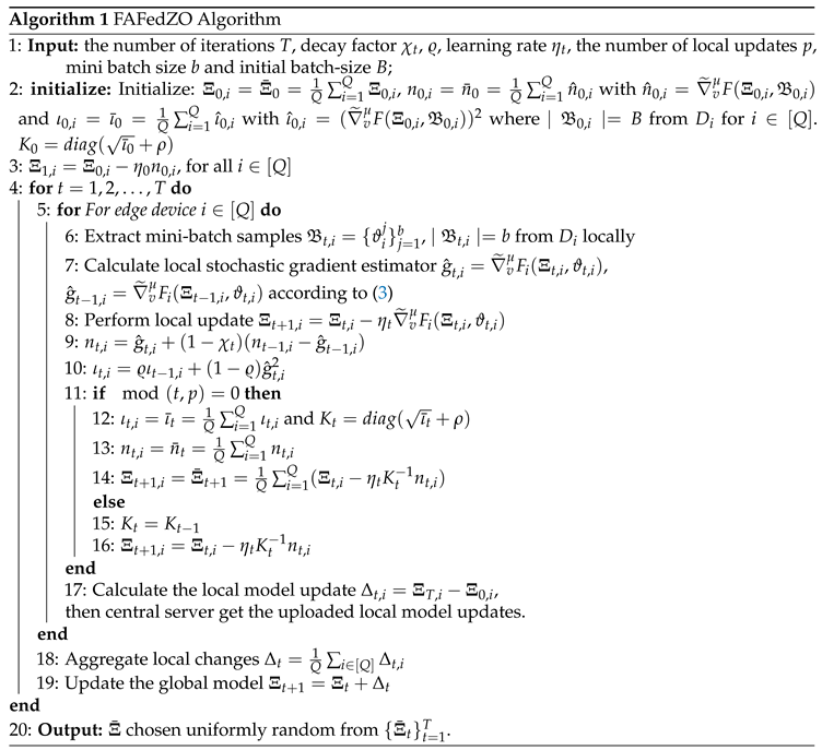
Firstly, we expand our algorithm description within the context of the FedAvg framework. We are focused here on solving problem (1) through zeroth-order optimization methods and propose a novel zero-order fast adaptive FL method (FAFedZO) employs a shared adaptive learning rate to address the issues. In particular, Algorithm 1 outlines the specifics of our FAFedZO method.
At the beginning, input the parameters and perform initialize. For all i, compute , which represents the first model update based on the initial parameters and the initial gradient estimates.
Then, for each edge device i, perform the following steps: First, extract a mini-batch of size b from the local dataset . Next, compute the stochastic gradient estimates and for the current model parameters based on the mini-batch . Here, we elaborate on the specific method for estimating the gradients.
To address the issue of unavailable gradient information and reduce the frequency of model exchange, we achieve this by using gradient estimators and performing stochastic zero-order updates in each communication round. In particular, at the t-th round, edge device i calculates a two-point stochastic gradient estimator [28] as outlined below
where denote the local model of edge device i, while signifies a random variable drawn by edge device i according to its local data distribution during the t-th round. represents a randomly chosen d-dimensional direction, uniformly sampled from the unit sphere , while stands for a positive step size.
When computing gradient estimates, we do not directly use precise gradient information but instead approximate the gradient through random sampling and estimation. This zero-order optimization approach does not require the exact calculation of function derivatives, rather, it optimizes based on sampling and estimation of function values.
Afterward, we update local models according to the following stochastic zeroth-order update method
where denotes the learning rate.
In step 9 of Algorithm 1, we use to update the model, where is the momentum-based variance reduced gradient estimator, is the weighted sum of the current gradient estimate and previous gradient estimates, with the weights determined by . Its definition is as follows
where the hyperparameter , representing the decay factor.
In step 10 of Algorithm 1, we incorporate the coordinate-wise adaptive learning rate approach, akin to that utilized in Adam [32], which is defined as follows
where the hyperparameter , representing the decay factor.
Then, when the current iteration number t is an integer multiple of the local update number p (i.e., ), we perform step 12.
In step 12 of Algorithm 1, for , we perform averaging and aggregation step and resulting in . Subsequently, we utilize the to create an adaptive matrix (where denotes diagonal matrix), and where ( represent tuning parameter).
At the step 13 in algorithm 1, perform averaging and aggregation on all nodes of .
In step 14, the global model is updated based on the obtained and .
Otherwise, proceed to steps 15 and 16 of the algorithm. Keep as its previous value and update the global model in the same manner as before.
In step 16 of algorithm 1, the identical is employed for the local updates across various edge devices.
Here, model parameters, , are aggregated by the global server every interval of p steps.
At the step 17 in algorithm 1, all edge devices calculate the model difference of their local models in the current round, that is, (, represents all Q edge devices from 1 to Q), uploaded to the central server.
At the step 18, 19 in Algorithm 1, after receiving the local model difference, central server summarizes it as , and proceeds to update the global model, that is .
Finally, after all iterations are completed, the algorithm outputs a model , which is uniformly randomly selected from all the global models obtained during the iterations, as the final result.
In the algorithm, is a diagonal matrix whose diagonal elements are related to , which is computed based on certain statistics from the local model update process. Specifically, is related to the square of the gradient estimates, and is obtained by averaging across all devices. Subsequently, is updated accordingly. This approach allows to adaptively adjust based on the variations in gradient information during the local model update process.
During the model training process, the data distribution on different devices may vary, leading to differing updates in model parameters. By adaptively updating , it is possible to influence the aggregation and update methods of the global model. For instance, when the gradient variation on a particular device is significant (i.e., is large), the value of will also change accordingly, thereby assigning different weights to the amount of updates from this device when aggregating local updates. This enables the algorithm to better adapt to the data distribution and model training situations on different devices, accelerating the convergence speed of the model and enhancing the final model performance.
4. Convergence Analysis of FAFedZO Method
For this part, the convergence of FAFedZO method will be discussed. To facilitate the theoretical analysis of the proposed algorithm, we need to make some assumptions as follows.
Assumption A1.
The global loss function in (1) has a lower bound, that is, there is a fixed value that exists
The Assumption 1 means that regardless of the value of the optimization variable , the global loss function will not decrease indefinitely, and there exists a minimum value , ensuring that the optimization problem is meaningful.
Assumption A2.
We suppose that function are all L-smooth, that is, for all , we can conclude that
The Assumption 2 is common in the theoretical analysis of non-convex optimization, indicating that the gradient changes of , are smooth and do not change suddenly, which is crucial for proving the convergence of algorithms.
Assumption A3.
serves as a precise approximation of without bias, namely
The Assumption 3 allows us to use sample gradients to approximate the true gradient.
Assumption A4.
The variance of the stochastic gradient is limited within a certain range, that is, there have a fixed value can satisfies
The Assumption 4 indicates that the variance of stochastic gradients will not be infinite, which is important for controlling noise and uncertainty in the optimization process.
Assumption A5.
The difference between each local loss function and the global loss function remains within a certain limit, that is, there have a fixed value can satisfies
The Assumption 5 ensures that local optimization does not lead to a significant decrease in global performance.
Assumption A6.
The inter-node variance is bounded, namely
The Assumption 6 indicates that the differences between loss functions on different nodes are limited, ensuring that the optimization processes on different nodes do not diverge too much.
Assumption A7.
In our algorithms, for all , the adaptive matrices satisfies the condition that
there ρ represents an appropriate positive value.
The Assumption 7 guarantees the step size in the optimization process does not become too small, thereby guaranteeing the convergence of the algorithm.
Assumption A8.
The gradients of function is G-bounded, that is, for all i, , we have
The Assumption 8 means that the gradients of the loss functions on each node are not infinite, ensuring stability and controllability in the optimization process.
We define the -stationary point as follows:
Definition 1.
A point Ξ is called ϵ-stationary point if . Generally, a stochastic algorithm is defined to achieve an ϵ-stationary point in T iterations if .
Then, we investigate the convergence characteristics of our novel method based on Assumptions 1-8. The Appendix A contains the comprehensive proofs of our results.
About the convergence of the FAFedZO algorithm, we present the main results of this paper as follows:
Theorem 1.
Assuming that the sequence is produced by Algorithm 1. Based on the aforementioned Assumptions 1-8, given that , , , , and set
we can conclude that
where
Remark 1.
We utilize ζ as an indicator of data heterogeneity. The final results demonstrate that an increase in ζ (indicating greater data heterogeneity) leads to a slowdown in the training process. In addition, as the parameters L and μ increase, the boundary in the theorem conclusion will also increase, which will also result in a decrease in the training speed.
Remark 2.
A suitable value of ρ ensures a balanced incorporation of adaptive information in the learning rate. In practice, we commonly select ρ to be within the order of , steering clear of excessively small or large values.
Analysis of computational complexity and convergence speed
(computational complexity) For , we have
without loss of generality, we let , and choose . To make the right side of the inequality less than , we can get and . Therefore, to satisfy the definition of an -stationary point, which is and , we obtain the total sample cost as and the communication round as .
(convergence speed) In the FedZO algorithm, when full devices participate, it can satisfy
when partial devices participate, it can satisfy
Regardless of the situation, we can observe that the FedZO algorithm achieves the convergence rate of . Furthermore, as indicated by Theorem 1, our algorithm can achieve the convergence rate of . Therefore, our FAFedZO method theoretically possesses a faster convergence rate compared to general zero-order methods. This further validates the advantages of our approach.
5. Experimental Results
For this part, we are conducting comparative experiments on the MNIST and CIFAR-10 datasets, present some experimental outcomes to assess the performance of the proposed FAFedZO method in federated black-box attacks, thereby confirming the advantages of this algorithm.
Experimental environment and datasets
Experimental environment configuration: This study utilizes the FedZO framework as the experimental baseline to conduct research on federated learning algorithms. This framework is renowned for its exceptional scalability and operational convenience, supporting numerous prominent federated learning algorithms. For this study, Python version 3.10.13 is adopted as the programming language, and PyTorch serves as the development platform. All tests are conducted on a Windows 10 platform equipped with an NV GTX1650 GPU and CUDA version 12.4.99.
Dataset: By conducting comparative experimental studies on the MNIST and CIFAR-10 datasets respectively, we have validated the practicality of the FAFedZO algorithm while significantly enhancing the performance of the model.
MNIST (Modified National Institute of Standards and Technology) is a widely used benchmark dataset for evaluating and comparing the performance of handwritten digit recognition algorithms. It was adapted by Professor Yann LeCun and his colleagues at New York University in 1998 from an original dataset of the National Institute of Standards and Technology (NIST). This dataset comprises a collection of grayscale images of handwritten digits (0-9) with 60,000 training samples and 10,000 test samples, each image measuring 28pixels. Each image has undergone a preprocessing pipeline, including centering and normalization, aimed at enhancing the accuracy of classification algorithms. The MNIST dataset is extensively utilized for training and testing image processing and machine learning algorithms, particularly as a classic dataset for introductory deep learning and neural network research. An example of this dataset is shown in Figure 1.
CIFAR-10 (Canadian Institute For Advanced Research-10) is a commonly used dataset in computer vision, particularly for image classification tasks. It is consist of 60,000 32x32 color images across 10 categories and each category contains 6,000 images, and the dataset is divided into 50,000 training and 10,000 test images. Due to its smaller image size and fewer categories, it is often used for rapid verification, prototype development, as well as learning and understanding the basics of various computer vision algorithms. It is also employed as a benchmark dataset for deep learning models to assess their performance and generalization ability on image classification tasks.
Experimental result analysis
Here, we present the results of simulation experiments to assess the performance of the FAFedZO method in the context of black-box attack strategies.
Given the characteristics of black-box scenarios, optimizing black-box attacks falls into the realm of zero-order optimization. We investigate black-box attacks on a trained deep neural network(DNN) classification model. The purpose of our experiment is to train an interference image with the same size as the image in the dataset, which makes it difficult for the human eyes to recognize the difference between the original image and the adversarial image after adding the interference image, but it can induce the classification model to make a wrong judgment. We want to achieve a higher attack success rate with as little disturbance as possible, so we consider the loss function as shown below:
Here represents the interference image to be trained, represents the original image in the dataset, and represents the label corresponding to the image (for example, the label of the image "deer" is 4) , represents the confidence that the classification model recognizes image as label j. I in (8) formula measures the probability of attack failure (marked as attack loss), represents the image distortion caused by disturbance, and c is the balance coefficient. In this way our goal can be achieved by minimizing . Next we use the (8) formula to construct the local loss function.
We divide the samples in the dataset into Q groups randomly and unevenly without repetition, and then distribute them to each edge device, where Q is the total count of edge devices we preset. Then for all edge devices we define its local loss function as:
Where represents the dataset at the ith edge device. In this way, the federal black-box attack problem on the DNN classification model can be formulated as a federated optimization problem: . Next, we use the FAFedZO algorithm proposed in this paper to solve this problem.
We select balance parameter . And for the remaining parameters, we select them as .
In Figure 2, we demonstrate the change in the accuracy of the federated black-box attack as the number of communication rounds increases. Figure (a) illustrates the impact of the account of local updates on attack accuracy of the proposed FAFedZO algorithm when the total number of edge devices and the number of participating edge devices . We also compare it with the FedZO algorithm. It can be observed that the larger the E value, the higher the attack accuracy of the algorithm. Furthermore, the attack accuracy of FAFedZO is significantly higher than that of FedZO. When , they achieve comparable accuracy, proving that the algorithm proposed in this paper outperforms the original FedZO algorithm. Figure (b) shows how the convergence performance of the FAFedZO method is affected by the number of participating edge devices when and . It can be seen that by adjusting the M value, the FAFedZO algorithm can effectively enhance the attack accuracy.
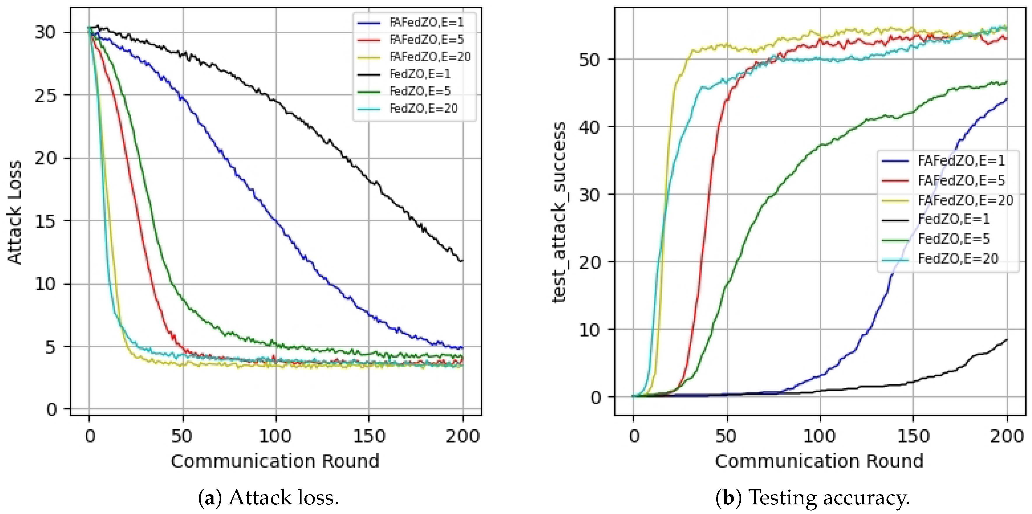
In Figure 3, we present the relationships between attack loss and communication rounds as well as attack accuracy and communication rounds, respectively. The influence of the number of local updates on the convergence performance of the algorithm is studied under the condition of and , i.e., all devices participate. It is evident that the FAFedZO scheme is capable of significantly decreasing the attack loss and improve attack accuracy compared to the FedZO algorithm under different E values. Moreover, as the value of E increases, the convergence speed of the FAFedZO algorithm also accelerates, with lower attack loss and higher attack accuracy, both of which tend to stabilize faster.
Figure 4 also shows the relationship between attack loss, attack accuracy, and communication rounds. However, we study how the number of participating edge devices influences the convergence performance of the scheme under the condition of and . It is easy to see that the FAFedZO algorithm is far superior to the FedZO algorithm in terms of both attack loss and accuracy. Even when the FedZO algorithm takes the optimal value of M among 10, 20, and 50, its performance is still weaker than the worst value of the FAFedZO algorithm. In addition, as M increases, the attack loss value decreases, and the accuracy increases, which is in line with our expectations.
The aforementioned experiments were all conducted on the MNIST dataset, and similar conclusions were also drawn from experiments performed on the CIFAR-10 dataset. As shown in Figure 5, under the conditions of and , the impact curves of the number of local updates on attack loss and accuracy are presented. It is evident that by adjusting the E value, the performance of the FAFedZO algorithm can also be significantly enhanced.
In addition to investigating the impact of the number of local updates and the number of participating edge devices on the algorithm’s performance, we also studied the influence of varying the number of random directions on the proposed algorithm. As shown in Figure 6, on the MNIST dataset, under the conditions of and , we present the curves illustrating the impact of the number of directions on attack loss and attack accuracy. It can be observed that we have similar conclusions to the above figures, which further confirms the superiority of the FAFedZO algorithm.
In addition, we also discuss the performance of our algorithm under the setting of non-independent and identically distributed (non-iid) data.
Figure 7 presents the impact of the number of local updates on the attack loss and accuracy of the algorithm under the non-iid setting. It can be observed that, compared with Figure 2, the attack accuracy in this case is lower than that under the iid setting, which is attributed to the influence of the non-iid setting and aligns with our expectations. Furthermore, the results also indicate that under the non-iid setting, the performance of the FAFedZO algorithm remains superior to that of the FedZO algorithm, and both achieve comparable performance levels when .
6. Discussion
Our approach combines zeroth-order optimization with adaptive techniques, yielding significant benefits in various real-world applications. For instance, in healthcare, medical data contains sensitive patient information and varies across different regions and hospitals. Utilizing this method allows the model to automatically adapt to these variations during training. Additionally, zeroth-order optimization can be leveraged to explore better solutions, enhancing the model’s generalization capability across diverse medical scenarios and improving its assistance in disease diagnosis. In the financial sector, financial institutions need to accurately identify risks such as fraudulent transactions. By employing this method, risk characteristics can be adaptively captured from vast amounts of financial transaction data, and zeroth-order optimization can be used for efficient optimization, thereby improving the accuracy of risk identification and preventing financial risks. In the realm of IoT devices, where resources are limited, zeroth-order optimization eliminates the need for gradient computation, reducing computational load. Adaptive methods can adjust training strategies based on device resources and data characteristics, enabling federated learning to operate efficiently on IoT devices and enhancing their data processing capabilities.
7. Conclusion
In this paper, we proposed FAFedZO, a zero-order federated optimization method based on an adaptive approach with a shared adaptive learning rate. In the non-convex setting, when gradient information is not available, FAFedZO can estimates the first-order gradient information through function queries to optimize the objective function. We have combined the advantages of zero-order optimization and adaptability. Zero-order estimation can solve the problem that the objective function is not available, thus the gradient information is not usable. Adaptability can accelerate the performance of the algorithm. Furthermore, our theoretical analysis of the algorithm demonstrates the convergence of FAFedZO. Finally, we conducted extensive experiments to verify the effectiveness of the proposed algorithm again on the MNIST and CIFAR-10 datasets, respectively.
Author Contributions
All authors have read and agreed to the published version of the manuscript.
Funding
This work was supported by Key Technologies Research and Development Program of Henan Province under Grant No. 242102210102.
Data Availability Statement
Data are contained within the article.
Conflicts of Interest
The authors declare there is no conflicts of interest.
Appendix A
Here, we present a thorough examination of our algorithm’s convergence properties. To facilitate the analysis, we introduce the notation that in the subsequent sections. Define as and use ⊗ as Kronecker product symbol. Below are some basic lemmas required for our analysis.
At first, for the zeroth-order gradient , based on the characteristics of the gradient estimator outlined in [38], Lemma 4.2], we can deduce that
Then, we can get
where the second equality is due to Assumption 3, the establishment of these four inequalities is because , [38], Lemma 4.1] and Assumption 4, Assumption 8.
Thus, we can get
At the same time, we can also obtain
The following Lemma A1 is a small conclusion throughout the proof.
Lemma A1
([39]).
Given and , there represents the vector composed entirely of ones, we can get conclusion that
Then we continue to delve into the upper bound of the adaptive matrices .
Lemma A2.
Suppose the adaptive matrices sequence is derived from Algorithm. On the Basis of Assumptions 1 to 8, we can conclude that
Proof. Firstly, we know that
there is a diagnoal matrix. And following the definition of , we can deduce that
Therefore, because of , taking the recursive expansion we can get
So we finally got
Lemma A2 is proved. □
The following Lemma A3 measures the boundary of variance between gradients.
Lemma A3.
For , represents all Q edge devices from 1 to Q, we can conclude that
Proof. For inequality (A9), we have
where the first inequality is because , the last inequality follows by [28], Lemma 5.2].
For inequality (A10), we have
the last two inequalities here are attributed to Assumption 2, 6.
Thus lemma A3 is proved. □
Below, we study the bounds under different values of , which is important for the proof of the subsequent theorems.
Lemma A4.
Given that , is derived from the Algorithm, we can conclude that
(1) if , then we can get
(2) if , then we can get
Proof.
(1) , then we can conclude that , so there is , thus we have obtained the final result.
(2) we have
thus
Lemma A4 is proved. □
The following lemmas A5-A7 are crucial conclusions that will be used in proving the final theorem.
Lemma A5.
Assuming the sequence is generated by the Algorithm, then we can get
Proof.
Regarding (1), we can obtain
Regarding term (2), , . We can obtain based on the given definition of and assumption 7 that
So
Bring (A20), (A18) into (A17), we can get
We considering the last term in (A21), taking expectation on both sides have
By substituting it into (A21), then taking the expectation of both sides, we can get this conclusion.
Lemma A5 is proved. □
Lemma A6.
Suppose that are produced by the Algorithm, we subsequently obtain
Proof. We know that
So we can get
where the last inequality is because the L-smoothness and Lemma A3.
Lemma A6 is proved. □
Lemma A7.
Suppose that are produced by the Algorithm, we subsequently obtain
Proof.
there (A26) arises is because the fact that . Continuing to process the latter term in (A26) yields
the last two inequalities here are attributed to Lemma A1 and the L-smoothness. Regarding the last term, we can get
the last two inequalities here are attributed to Lemma A1 and Lemma A3. Then, by integrating the aforementioned inequalities (A28), (A27), (A26) with the definition of , we can deduce that when , the following formula can be reached.
where we utilize the Lemma A4. Then combine like terms we have
We select , and we know that , then
On the other hand, if that is , it follows that . So taking the recursive expansion to (A32), we have
where we utilize that and . Then by multiplying both sides by we can get
Finally,
where the last inequality is because so that .
Therefore,
Given that and . By multiply on both side, we can get
Lemma A7 is proved. □
Proof of Theorem
Now let’s prove the final theorem.
Proof. We set , , , and . So we can infer that
It is clear that . And
where we leverage the concavity of , that is , the second inequality is valid because of and the last inequality is obtained based on .
where the second inequality holds true because and , and the last inequality is obtained based on (A38). Therefore, we have
Subsequently, we set
where we utilize that Lemma A4, Lemma A5 and . By summing the results from to , where , then can obtain
here, by utilizing Lemma A7 and the fact that , we can derive the last inequality. Subsequently, summing the terms from the start can obtain
Furthermore, we can obtain
Then consider that , since . Taking Lemma A3 and dividing both sides of the above result by can get
Regarding the first term in (A45),
For the middle term, we have
For the third term
We let
and if we choose , then , , . So we can infer that it is convergent.
Then with Jensen’s inequality and can get
Finally,
where we utilize Young’s inequality and ,
and .
Since is convergent as mentioned before, it can be known that is also convergent, thus the theorem is proved. □
References
- McMahan, B.; Moore, E.; Ramage, D.; Hampson, S.; y Arcas, B.A. Communication-efficient learning of deep networks from decentralized data. In Proceedings of the Artificial intelligence and statistics; 2017; pp. 1273–1282. [Google Scholar]
- Shi, Y.; Yang, K.; Yang, Z.; Zhou, Y. Mobile edge artificial intelligence: Opportunities and challenges 2021.
- Yang, L.; Tan, B.; Zheng, V.W.; Chen, K.; Yang, Q. Federated recommendation systems. Federated Learning: Privacy and Incentive, 2020, pp. 225–239.
- Yang, K.; Shi, Y.; Zhou, Y.; Yang, Z.; Fu, L.; Chen, W. Federated machine learning for intelligent IoT via reconfigurable intelligent surface. IEEE network 2020, 34, 16–22. [Google Scholar] [CrossRef]
- Tian, J.; Smith, J.S.; Kira, Z. Fedfor: Stateless heterogeneous federated learning with first-order regularization. arXiv.2209.10537 2022. [Google Scholar]
- Zhang, M.; Sapra, K.; Fidler, S.; Yeung, S.; Alvarez, J.M. Personalized federated learning with first order model optimization 2021.
- Elbakary, A.; Issaid, C.B.; Shehab, M.; Seddik, K.G.; ElBatt, T.A.; Bennis, M. Fed-Sophia: A Communication-Efficient Second-Order Federated Learning Algorithm. arXiv.2406.06655 2024. [Google Scholar]
- Dai, Z.; Low, B.K.H.; Jaillet, P. Federated Bayesian optimization via Thompson sampling. Advances in Neural Information Processing Systems 2020, 33, 9687–9699. [Google Scholar]
- Fang, W.; Yu, Z.; Jiang, Y.; Shi, Y.; Jones, C.N.; Zhou, Y. Communication-efficient stochastic zeroth-order optimization for federated learning. IEEE Transactions on Signal Processing 2022, 70, 5058–5073. [Google Scholar] [CrossRef]
- Li, Z.; Ying, B.; Liu, Z.; Yang, H. Achieving Dimension-Free Communication in Federated Learning via Zeroth-Order Optimization. arXiv.2405.15861 2024. [Google Scholar]
- Maritan, A.; Dey, S.; Schenato, L. FedZeN: Quadratic convergence in zeroth-order federated learning via incremental Hessian estimation. In Proceedings of the 2024 European Control Conference; 2024; pp. 2320–2327. [Google Scholar]
- Staib, M.; Reddi, S.; Kale, S.; Kumar, S.; Sra, S. Escaping saddle points with adaptive gradient methods. In Proceedings of the International Conference on Machine Learning; 2019; pp. 5956–5965. [Google Scholar]
- Chen, X.; Li, X.; Li, P. Toward communication efficient adaptive gradient method. In Proceedings of the Proceedings of the 2020 ACM-IMS on Foundations of Data Science Conference, 2020, pp. 119–128.
- Reddi, S.; Charles, Z.; Zaheer, M.; Garrett, Z.; Rush, K.; Konečnỳ, J.; Kumar, S.; McMahan, H.B. Adaptive federated optimization. arXiv:2003.00295, 2020. [Google Scholar]
- Wang, Y.; Lin, L.; Chen, J. Communication-efficient adaptive federated learning. In Proceedings of the International Conference on Machine Learning; 2022; pp. 22802–22838. [Google Scholar]
- Wang, J.; Liu, Q.; Liang, H.; Joshi, G.; Poor, H.V. A novel framework for the analysis and design of heterogeneous federated learning. IEEE Transactions on Signal Processing 2021, 69, 5234–5249. [Google Scholar] [CrossRef]
- Li, T.; Sahu, A.K.; Zaheer, M.; Sanjabi, M.; Talwalkar, A.; Smith, V. Federated optimization in heterogeneous networks. Proceedings of Machine learning and systems 2020, 2, 429–450. [Google Scholar]
- Karimireddy, S.P.; Kale, S.; Mohri, M.; Reddi, S.; Stich, S.; Suresh, A.T. Scaffold: Stochastic controlled averaging for federated learning. In Proceedings of the International conference on machine learning; 2020; pp. 5132–5143. [Google Scholar]
- Pathak, R.; Wainwright, M.J. FedSplit: An algorithmic framework for fast federated optimization. Advances in neural information processing systems 2020, 33, 7057–7066. [Google Scholar]
- Zhang, X.; Hong, M.; Dhople, S.; Yin, W.; Liu, Y. Fedpd: A federated learning framework with adaptivity to non-iid data. IEEE Transactions on Signal Processing 2021, 69, 6055–6070. [Google Scholar] [CrossRef]
- Wang, S.; Roosta, F.; Xu, P.; Mahoney, M.W. Giant: Globally improved approximate newton method for distributed optimization. Advances in Neural Information Processing Systems 2018, 31. [Google Scholar]
- Li, T.; Sahu, A.K.; Zaheer, M.; Sanjabi, M.; Talwalkar, A.; Smithy, V. Feddane: A federated newton-type method. In Proceedings of the 2019 53rd Asilomar Conference on Signals, Systems, and Computers; 2019; pp. 1227–1231. [Google Scholar]
- Xu, A.; Huang, H. Coordinating momenta for cross-silo federated learning. In Proceedings of the Proceedings of the AAAI Conference on Artificial Intelligence, 2022, Vol. 36, pp. 8735–8743.
- Das, R.; Acharya, A.; Hashemi, A.; Sanghavi, S.; Dhillon, I.S.; Topcu, U. Faster non-convex federated learning via global and local momentum. In Proceedings of the Uncertainty in Artificial Intelligence; 2022; pp. 496–506. [Google Scholar]
- Khanduri, P.; Sharma, P.; Yang, H.; Hong, M.; Liu, J.; Rajawat, K.; Varshney, P. Stem: A stochastic two-sided momentum algorithm achieving near-optimal sample and communication complexities for federated learning. Advances in Neural Information Processing Systems 2021, 34, 6050–6061. [Google Scholar]
- Jiang, W.; Han, H.; Zhang, Y.; Mu, J. Federated split learning for sequential data in satellite-terrestrial integrated networks. Information Fusion 2024, 103, 102141. [Google Scholar] [CrossRef]
- Jiang, W.; Han, H.; Zhang, Y.; Mu, J.; Shankar, A. Intrusion Detection with Federated Learning and Conditional Generative Adversarial Network in Satellite-Terrestrial Integrated Networks. Mobile Networks and Applications, 2024, pp. 1–14.
- Tang, Y.; Zhang, J.; Li, N. Distributed zero-order algorithms for nonconvex multiagent optimization. IEEE Transactions on Control of Network Systems 2020, 8, 269–281. [Google Scholar] [CrossRef]
- Nikolakakis, K.; Haddadpour, F.; Kalogerias, D.; Karbasi, A. Black-box generalization: Stability of zeroth-order learning. Advances in neural information processing systems 2022, 35, 31525–31541. [Google Scholar]
- Balasubramanian, K.; Ghadimi, S. Zeroth-order (non)-convex stochastic optimization via conditional gradient and gradient updates. Advances in Neural Information Processing Systems 2018, 31. [Google Scholar]
- Mhanna, E.; Assaad, M. Rendering Wireless Environments Useful for Gradient Estimators: A Zero-Order Stochastic Federated Learning Method. arXiv.2401.17460 2024. [Google Scholar]
- Diederik, P.K. Adam: A method for stochastic optimization 2014.
- Duchi, J.; Hazan, E.; Singer, Y. Adaptive subgradient methods for online learning and stochastic optimization. Journal of machine learning research 2011, 12. [Google Scholar]
- Ling, X.; Fu, J.; Wang, K.; Liu, H.; Chen, Z. Ali-dpfl: Differentially private federated learning with adaptive local iterations. In Proceedings of the 2024 IEEE 25th International Symposium on a World of Wireless, Mobile and Multimedia Networks; 2024; pp. 349–358. [Google Scholar]
- Cong, Y.; Qiu, J.; Zhang, K.; Fang, Z.; Gao, C.; Su, S.; Tian, Z. Ada-FFL: Adaptive computing fairness federated learning. CAAI Transactions on Intelligence Technology 2024, 9, 573–584. [Google Scholar] [CrossRef]
- Huang, Y.; Zhu, S.; Chen, W.; Huang, Z. FedAFR: Enhancing Federated Learning with adaptive feature reconstruction. Computer Communications 2024, 214, 215–222. [Google Scholar] [CrossRef]
- Li, Y.; He, Z.; Gu, X.; Xu, H.; Ren, S. AFedAvg: Communication-efficient federated learning aggregation with adaptive communication frequency and gradient sparse. Journal of Experimental & Theoretical Artificial Intelligence 2024, 36, 47–69. [Google Scholar]
- Gao, X.; Jiang, B.; Zhang, S. On the information-adaptive variants of the ADMM: an iteration complexity perspective. Journal of Scientific Computing 2018, 76, 327–363. [Google Scholar] [CrossRef]
- Wu, X.; Huang, F.; Hu, Z.; Huang, H. Faster adaptive federated learning. In Proceedings of the Proceedings of the AAAI conference on artificial intelligence, 2023, Vol. 37, pp. 10379–10387.
Figure 1.
Example of the MNIST dataset.
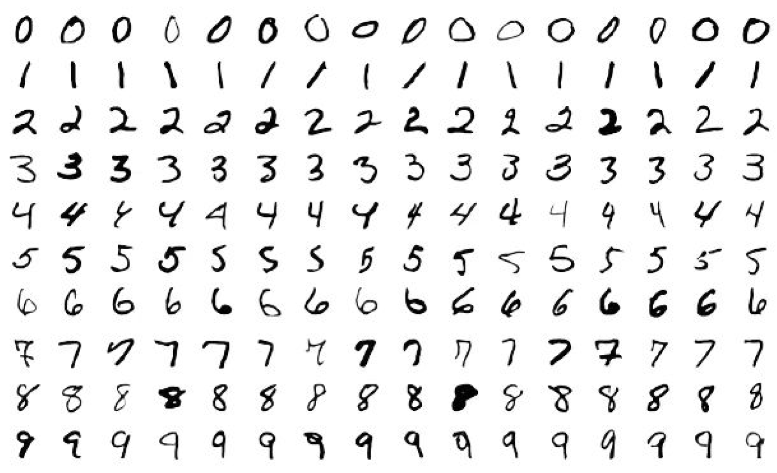
Figure 2.
Federated black-box attack accuracy against the number of communication rounds.
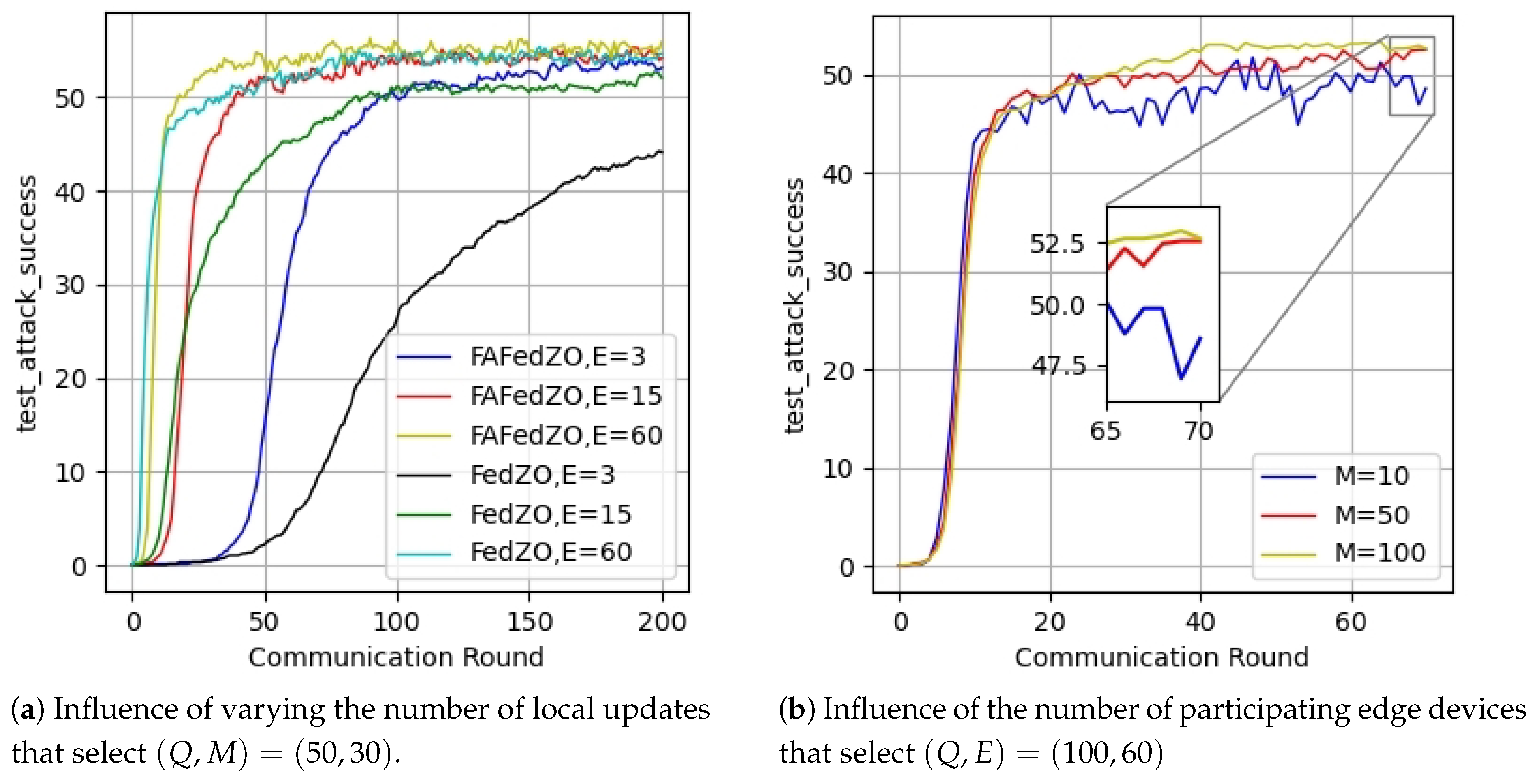
Figure 3.
Influence of the number of local updates that select and .
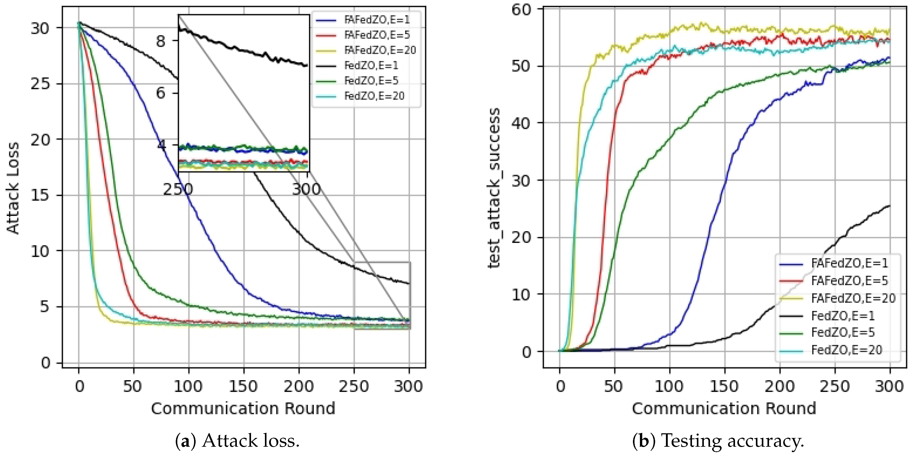
Figure 4.
Influence of the number of participating edge devices that select and .
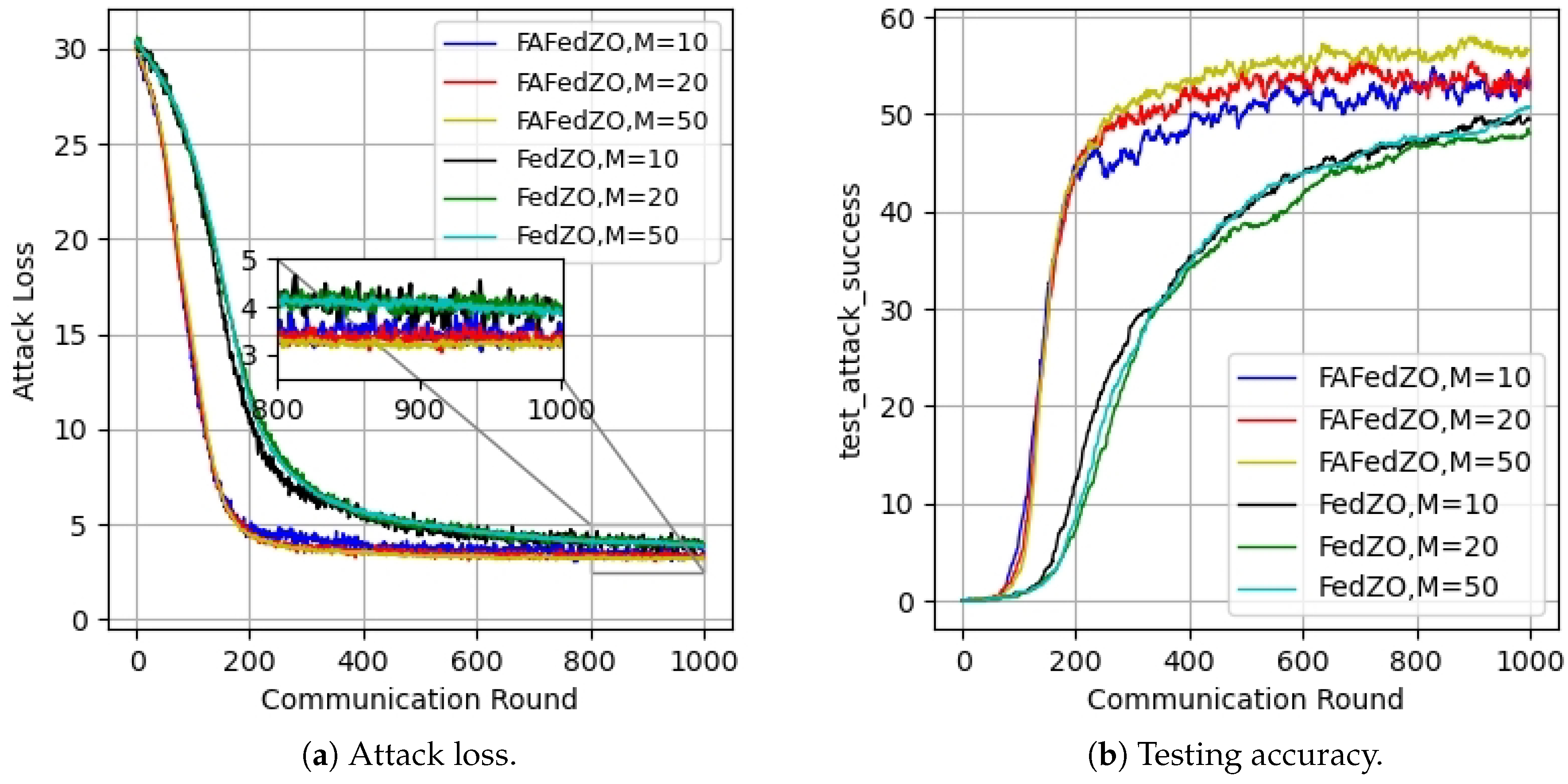
Figure 5.
Influence of the number of local updates that select and .
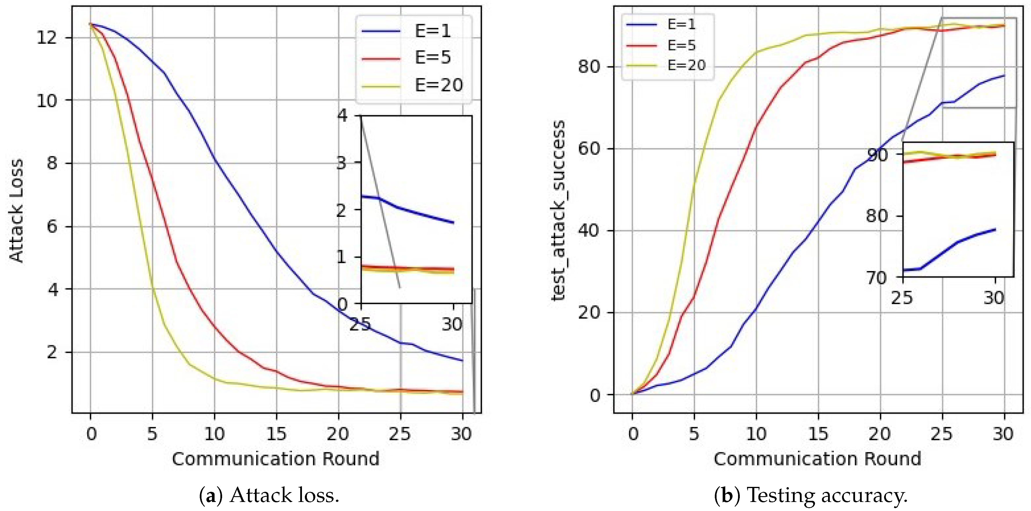
Figure 6.
Influence of the number of directions that select and .
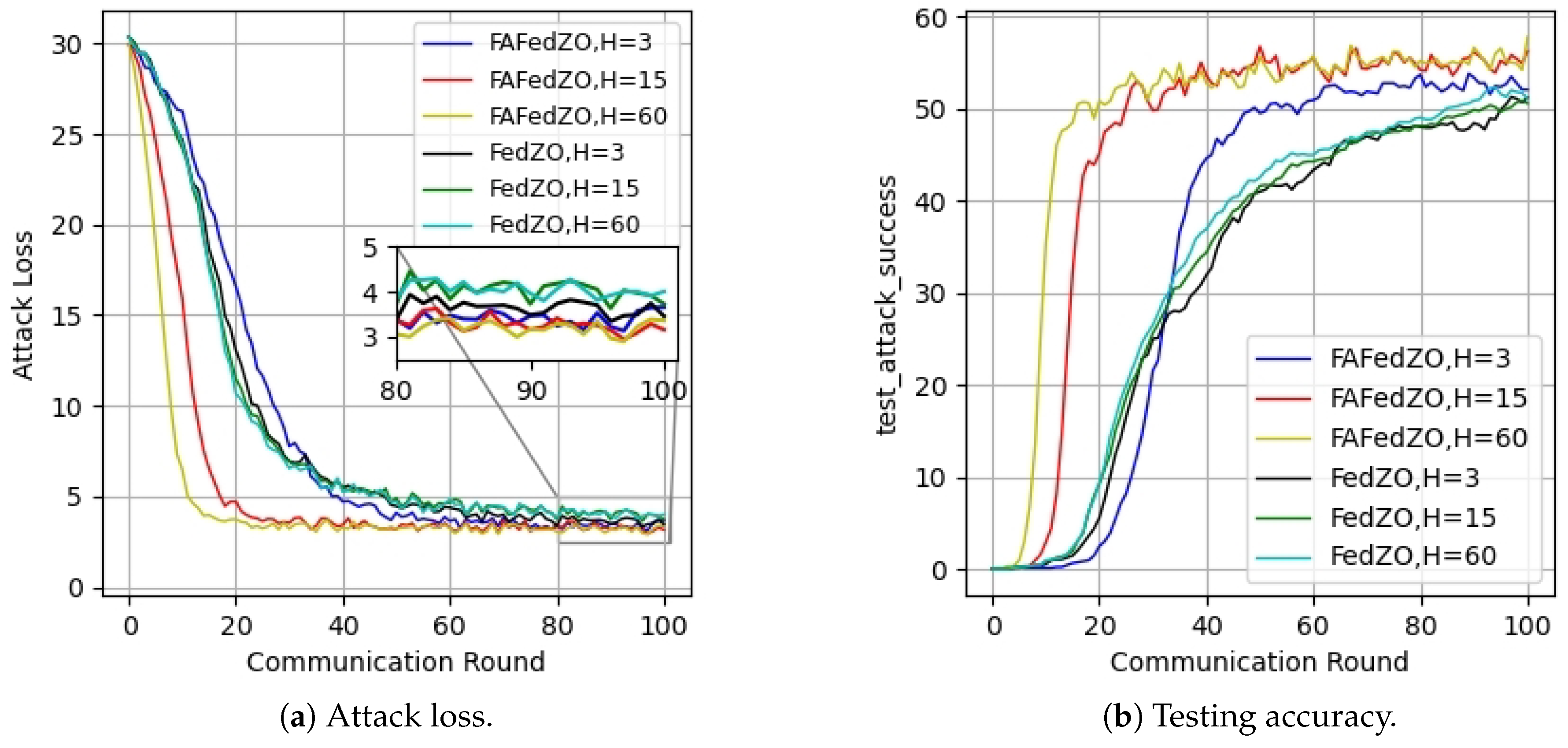
Figure 7.
The impact of different numbers of local updates when selecting and in a non-IID setting.
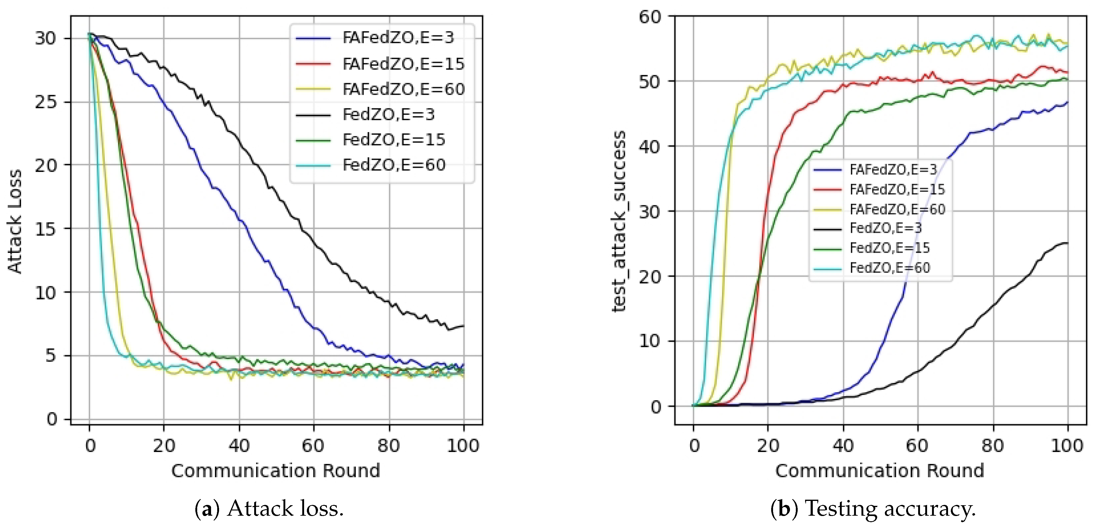
Figure 8.
The impact of the number of participating edge devices when selecting and under the non-IID setting.
Figure 8.
The impact of the number of participating edge devices when selecting and under the non-IID setting.
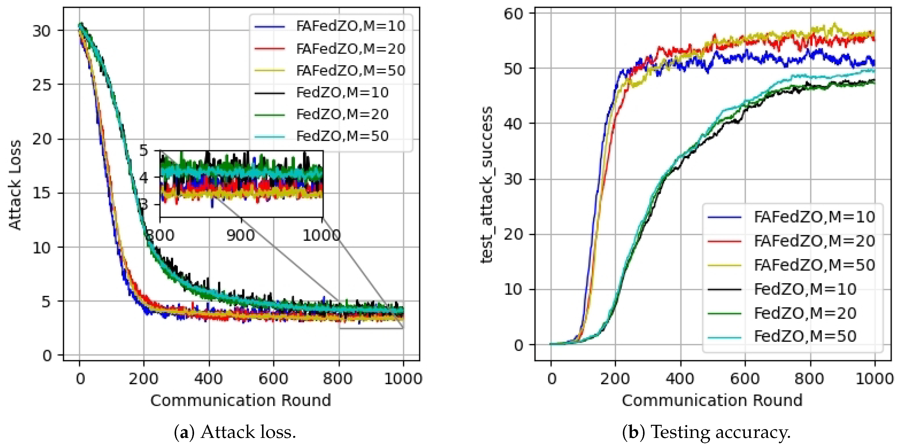
Figure 9.
The impact of different numbers of local updates when selecting and under the non-IID setting.
Figure 9.
The impact of different numbers of local updates when selecting and under the non-IID setting.
Disclaimer/Publisher’s Note: The statements, opinions and data contained in all publications are solely those of the individual author(s) and contributor(s) and not of MDPI and/or the editor(s). MDPI and/or the editor(s) disclaim responsibility for any injury to people or property resulting from any ideas, methods, instructions or products referred to in the content. |
© 2025 by the authors. Licensee MDPI, Basel, Switzerland. This article is an open access article distributed under the terms and conditions of the Creative Commons Attribution (CC BY) license (http://creativecommons.org/licenses/by/4.0/).
Copyright: This open access article is published under a Creative Commons CC BY 4.0 license, which permit the free download, distribution, and reuse, provided that the author and preprint are cited in any reuse.


