
Submitted:
20 January 2025
Posted:
21 January 2025
You are already at the latest version
Abstract
Advancements in the field of Artificial Intelligence has been rapid in recent years and has revolutionized various industries. Various deep neural network architectures capable of handling both text and images, covering code generation from natural language, producing machine translation and text summarizations have been proposed. For example, Convolutional Neural Networks or CNNs perform image classification at a level equivalent to that of humans on many image datasets. These state-of-the-art networks have reached unprecedented levels of success by using complex architectures with billions of parameters, numerous kernel configurations, weight initialization and regularization methods. Unfortunately to reach this level of success, the models that CNNs use are essentially black box in nature with little or no human interpretable information on the decision-making process. This lack of transparency in decision making gave rise to concerns amongst some sectors of the user community such as healthcare, finance, justice, defense, among others. This challenge motivated our research where we successfully produced human interpretable influential features from CNNs for image classification and captured the interactions between these features by producing a concise decision tree making accurate classification decisions. The proposed methodology made use of a pre-trained VGG16 with finetuning to extract feature maps produced by learnt filters. On the CelebA image benchmark dataset, we successfully produced human interpretable rules that captured the main facial landmarks responsible for segmenting males from females with 89.6% accuracy, while on the more challenging Cats vs Dogs dataset the decision tree produced 87.6% accuracy.
Keywords:
Convolutional Neural Network
; Decision Tree
; Feature Maps
; Image Classification
; Contour Extraction
1. Introduction
Artificial Intelligence has made significant progress, especially in recent years, where it has undergone unprecedented development and revolutionized various fields and industries by improving productivity in virtually every sector of Industry. Transitioning from a theoretical concept in the early 1950s [1], it has become a mainstream technology reaching a broader audience, through different applications used on a day-to-day basis. For instance, the recent surge in the usage of large language models capable of generating code from natural language, producing machine translations and performing text summarizations, exemplify the advancements in this field benefiting not only professionals but the general public as well.
In the last decade, a plethora of deep neural network architectures were proposed, with increasing complexities and greater depth in terms of layers. In addition, different kernel configurations, utilizing several different weight initialization and regularization methods enabled the use of deep learning with depths reaching thousands of layers with billions of learned parameters. These sophisticated architectures and techniques helped to reach unprecedented success in different benchmark tasks like ILSVRC [2] or CIFAR [3]. However, this race towards perfection with highly complex architectures [4-8] also transitioned the models into black-box entities which provided little or no information on the decision-making process employed by these models. These models, although performing very well in terms of accuracy, became opaque and the challenges of interpretation or explainability started raising concerns [9-12].
For some industries, such as healthcare, security, finance and justice, transparency in decision making is equally important, if not more so than accuracy. For instance, in healthcare, a deep learning model’s diagnosis with high accuracy provides an insight, however, explaining the decision-making process or the logic behind that conclusion is equally important to understand, to be acceptable and trustworthy to end-users. Introducing interpretability in complex models addresses transparency needs and bridges the gap between high performance and explainability of the decision-making process. The exploration and improvement have given rise to a vigorous, yet nascent field of research known as eXplainable Artificial Intelligence (XAI) which seeks to enhance transparency, accountability and trust in AI systems [13,14].
The body of research in XAI [15-19] has given rise to partial success in explaining decisions taken by CNNs in the application domain area of image classification. The focus has been on using feature maps to explain decisions taken by the classifier at the output layer. Some examples include local eXplainable AI (XAI) methods such as Layer-wise Relevance Propagation (LRP) [17], global XAI techniques providing insights through visual explanations (heatmaps) and model inspection, and an even more recent work, Concept Relevance Propagation (CRP) [18] which extended LRP to provide feature maps with richer content which in turn provided for more accurate explanations of classification decisions taken.
Despite the surge of interest in XAI there has been no attempt so far at capturing interactions between different features (in the form of feature maps). Local models focusing on individual features and recording their contribution in classifying images are useful in their own right but do not provide a comprehensive explanation of why one image is classified for example as a cat whereas another is categorized as a dog. What differentiates one type of image from another is a set of features along with the interactions between them. The objective of this research is to propose and validate a methodology that produces a transparent model that explains how classification decisions are made based on the set of features used and the interactions between them. The proposed methodology automatically extracts features from images and then constructs a decision tree based on this features that traces how classification decisions are made by following a decision path from the root of the tree down to the leaf node that identifies the class of the image.
2. Materials and Methods
2.1. Overview of methodology
Our methodology uses a 2-phase process. In phase 1, features are extracted from a CNN classification model. We describe our feature extraction method with reference to the VGG16[19] architecture, although our feature extraction method is generic and can be used with any CNN architecture.
Figure 1 displays the steps involved with feature extraction. The first step involves finetuning a pretrained model. The pretrained model that we used was Imagenet [20]. To finetune the model, we froze the weights obtained from the first 13 layers of the Imagenet model and re-trained the last k layers with our custom dataset. The optimal value of k was determined experimentally by tuning the CNN model on the validation set to obtain the highest classification accuracy. We will elaborate on this process in the detailed discussion that follows in section 2.2.1.
Finetuning helps to focus the training on the custom dataset and reduces the number of feature maps produced by the last convolutional layer. The feature maps in the last convolutional layer are the most significant amongst all other CNN layers as they are responsible for feeding the dense (classification layers) with the data required to make classification decisions. More details on the methodology, including the finetuning is in [21].
In the next step the feature maps identified through finetuning were processed to extract features. Feature maps are represented by 2 dimensional arrays and these arrays had to be further processed to obtain scalar valued features that could be fed into a decision tree model. The details of the transformation from 2d arrays to scalar form are presented in section 2.2.2.
In phase 2, the scalar features extracted were used to induce a decision tree model which was followed by encoding the decisions taken at the leaf nodes of the tree with symbolic rules that are human interpretable.
2.2. Feature extraction and rule generation
In this we describe the details of feature selection in section 2.2.1 and then go on to describe the rule generation processes in section 2.2.2
2.2.1. Feature extraction from feature maps
As described above the strategy used in feature extraction was to obtain a small number of feature maps by tuning the number of layers (k) that were re-trained using the target custom dataset. This resulted in reducing the number of feature maps responsible for classification from 512 to a small number. The value of k ranged between 1 (the layer closest to the first dense classification layer) to 3 (the layer furthest away from the dense layers) in block 5 of the VGG -16 architecture. The value of k that yielded the highest accuracy on the validation dataset was used to identify feature maps that consisted entirely of zero-valued activations. These feature maps were filtered out and the remaining maps were selected for feature extraction. We also validated the subset of feature maps that were selected against the set of feature maps F produced by VGG-16 without tuning – i.e., the original features maps at the last convolutional layer. With n as the number of feature maps produced by finetuning we randomly selected 2n, 3n, 4n, ….,mn feature maps from F and then for each subset selected we again evaluated the accuracy across the validation set. The integer m is given by m=floor(128/n) from set F where floor returns the smallest multiple of n that is smaller than 128. The rationale here was to demonstrate that the features returned from finetuning were far superior to randomly selecting up to a large fraction (25%) of the features from the original VGG-16 model without finetuning. In both datasets that we experimented with we found that the feature maps returned from feature selection were far superior to that of random selection from the original set F. In section 3 we present the detailed results of this experiment.
The next step of the methodology was to apply bilinear interpolation to scale each feature map (which is of size 8 by 8 for VGG-16) to the size of the original images (which is of size 128 by 128) for both datasets that we used. The intention here was to superimpose selected feature maps on the source images. Such superposition would enable us to identify which regions from the source images were responsible for classification by the CNN model. Having performed the superposition, we next performed a binarization operation to isolate significant regions from non-significant ones. To implement this, we used a threshold of 90% on the intensity of pixels to binarize the image. That is, we selected 90% of the brightest pixels from the superposed image to identify the areas of each image that were critical to classification by the CNN, which we term the critical region.
The contours of the critical region was then extracted for each feature map yielded irregular shapes which could not easily be represented by scalar features. To produce scalar features, we constructed the minimum bounding box that enclosed the critical region. With the minimum bounding box in place, we computed three scalar measures from it, namely aspect ratio, perimeter and area. These three measures taken together provide rotation invariancy of the critical region as they capture inherent geometry that is insensitive to the angular positioning of the critical region.
The final step in phase 1 was to provide locality information of critical regions relative to the dimensions of the original source image. To implement this, we divided the source image into a number of two-dimensional grids and then recorded the grid positions of each of the four vertices of the minimum bounding box. The motivation for this was to introduce interpretability into the features generated by providing spatial context that enables end users to understand the decision-making process. Thus, for example, with the CelebA dataset a feature located in the central part of the face such as the cheek helped to distinguish between males and females. Introduction of spatial context in terms of easily identifiable face landmarks is a necessary and powerful method of introducing transparency into the decision-making process used by the CNN.
3. Results
We experimented with two different datasets, namely the CelebA [22] and the Cats-vs-Dogs [23] dataset.
3.1. System Configuration
All experiments were conducted in the Google Collab environment using a paid subscription plan granting access to premium Nvidia's T4 GPUs without quota restrictions. Most of the experiments were executed using 15GB GPU memory and 12.7GB of system memory in the Python 3 environment. In certain exceptional situations, requiring high performance for testing purposes a 51GB of RAM was utilized. However, having high memory system is not required and 15GB GPU is sufficient to replicate the experiments (high memory was required for plotting feature maps using matplotlib and could be done with a 15GB RAM configuration as well, albeit with a time penalty).
A MacBook Pro with Intel processor and 8GB of RAM was used as a client machine to access google Collab in Chrome and Safari browsers. At least an 8GB machine is recommended as the browser running Collab notebook uses up to 3GB of memory at certain instances while plotting different feature maps.
3.2. Architecture Exploration
We present here the baseline CNN architecture which is used across both image datasets as a feature extractor. This baseline CNN uses certain hyperparameters which were finalized after conducting numerous experiments. For example, the method used to reduce the number of features extracted at the last block of VGG16 was to train the last few convolutional layers with the custom dataset (CelebA[] or Cats vs Dogs[], as the case may be). However, the question of how many layers to train in order to generate the smallest number of meaningful feature maps to achieve accuracy well above that obtained through random selection was finalized after multiple experimental runs covering multiple conv VGG16 layers of the last 2 blocks.
Similarly, other important hyperparameters such as the number of dense layers, number of units in each dense layer, learning rate, requirement of adaptive learning rate, number of epochs, early stopping, early stopping patience levels, optimizer, dimension of the input images, need for regularization covering L1, L2 and dropout, batch size and train, test & validation split were finalized after 100s of experimental runs. Once these parameters were chosen from the experiments, the same values were used throughout all experiments for different datasets otherwise mentioned specifically in the experiment sub-section. These parameter values are given below in Table 1 for reference:
3.3. Experimental Study
For each dataset we present the results of feature selection, image superposition, critical region extraction, feature generation, decision tree induction and finally symbolic rule generation. Before we describe experimentation in detail, we first present the system configuration we used to promote replicability.
We start with the experimentation on the CelebA dataset.
3.3.1. Finetuning, Feature Selection and Image Superposition
As described in section 2 finetuning was performed on the last two layers of the vgg-16 model and the feature maps that had activation values of non-zero were selected. Finetuning was highly effective on this dataset as we achieved a reduction from 512 maps to just 2.
In extracting contours from the critical regions, splitting was encountered in some cases, giving rise to two or more disjoint contours. Figure 2 displays the source image for sample number 6 in the male group, while Figure 3 displays the contours for feature maps 106 and 423, respectively.
Figure 3 shows clearly that map 106 for males captures the lower neck region whereas the chin, lower cheek and mouth regions is captured by map 423. Each of the two contours defined in maps 106 and 423 will give rise to three features defined by their respective minimum bounding rectangles, namely aspect ratio, perimeter and area.
We also display the source image for the sixth image in the female group and the resulting feature maps and their contours in
respectively.
Figure 5 shows some major differences with Figure 3. Firstly, the location of feature maps is distinct form those of male images. The female feature maps are located in three separate localities. Secondly, as shown in map 106 the upper shoulder area is highlighted which captures the long hair of a female. Map 106 also highlights another area which is the lower neck which was also highlighted in the male images. We also observe in map 106 an example of contour splitting with splits into three segments, as already described. Finally, we observe in map 423 that the distinctive female eyebrow is captured.
These same trends were observed for the Cats-vs-Dogs dataset. The images are appended to the Appendix due to space constraints.
Once contours were obtained for each feature map, bilinear interpolation [] was performed to scale up to the source image size and enable mapping to grid localities. An example of a grid mapped contour, and its corresponding features is shown in Figure 6.
As Figure 6 shows the contour straddles both the lower (G3 and G4) grids and hence the contour is named G3_G4_feature-map#, where feature-map# refers to the original feature map that gave rise to the contour at convolutional layer 17. An example of a contour is G3_G4_106_0, which in turn gave rise to 3 predictor features G3_G4_106_0_perimeter, G3_G4_106_0_area and G3_G4_106_0_aspect_ratio. As described in section 2 we used the 3 basic shape constructs of perimeter, area and aspect ratio to capture the predictive properties of a feature with the belief that given any two arbitrary contours X and Y, the combination of the 3 shape features will discriminate between X and Y to a high degree.
In summary, we observed clear differences between contours (which are basically our predictor features) across samples belonging to different classes. Moreover, as we can see from the images themselves the features are human interpretable and intuitive implying that a decision tree induced from such features will result in decision paths which end users can relate to, thus paving the way for introducing transparency.
We now induced a decision tree using the contours produced after gridding as described above. The decision tree induced on the CelebA dataset was produced by sklearn’s Decision Tree library and is shown in Figure 7.
In order to interpret the features produced by the tree we present in Figure 8 a sample of 8 images, with 4 examples from each class.
We validated the generated decision tree with the help of feature maps derived from earlier steps and then produced the following simple, yet informative rules that we condensed from the original rules produced by the tree.
Rule -1: If Lip and left Cheek perimeter is large and eyebrow area is small then Male, else Female.
Rule - 2: If Lip and left Cheek perimeter is small and Neck area is also small then Female, else Male.
Note: The original actual rules with decision tree threshold values are given below:
Rule -1: If Lip and left Cheek perimeter is > 105.305 and left eyebrow area is <= 7.5 then Male, else Female.
Rule - 2: If lip and left cheek perimeter is <= 105.305 and neck area is <= 710.5 then Female, else Male.
We now present our results on the Cats vs Dogs Dataset
Similar to the last experiment over the CelebA dataset, this experiment also follows the core methods to explain decision making from a CNN using baselined VGG16 with the same methodology of extracting a limited number of features. Our objective is to explain the features learnt to classify cats from dogs by tracing through decision trees with grids and contours annotating features.
The dataset used for this experiment contains 25,000 images of cats and dogs, each of varying pixel size. The attribute .csv file has only two features: image_id and the label (1=dog, 0=cat). No filters were applied and the whole dataset was used for training and prediction. We used 75% images are for training. Some sample images from each class are shown in Figure 9 and Figure 10.
Images were resized to the same dimension of 128x128x3 while normalization was done by dividing pixels values by 255. As with the CelebA dataset, a pretrained VGG16 model was used for training. Compared to the CelebA dataset, this dataset presented challenges with respect to variation in the size of images, variation in the degree of rotation, and in some cases obfuscation of the image caused by background objects. Due to such challenges, the pretrained CNN model returned a lower rate of 93.1% accuracy which fell short of the accuracy achieved with the CelebA dataset.
We followed the same approach as in CelebA to predict the test images and extract feature maps of dimension 8x8 from the last convolution layer. We then mapped the 8x8 feature maps to the 128x128 original images using interpolation with a threshold of 95%, whereby the intensity of the top 5% brightest pixels was set to value 255 and the rest to 0. Applying this threshold can result in disjointed contours, similar to the last experiment.
For each contour, the area, perimeter, coordinate and aspect ratio are computed by using coordinates (with height & width). We then translated these features to 2x2 grids (G1, G2, G3, G4) and changed feature names according to the grid coordinates these contours fell in.
New feature names were represented as G2_G4_94_0_perimeter, G2_G4_94_0_area, G2_G4_94_0_aspect_ratio and so on.
We then induced a decision tree on these features with the max_depth parameter set to 3 which achieved an accuracy of 87.6 % as shown in Figure 13.
Figure 13 shows that at Level 1, separation was by aspect ratio of face, with a smaller aspect ratio favouring cats with a high probability of 3694/5042 or 73.3%.
Amongst the sub population of animals having a smaller aspect ratio, a larger face area separated dogs from cats with a probability of 90.1%.
In total, a set of only 3 features turned out to be needed for separating cats from dogs with 87.6% accuracy.
4. Discussion
With images that had consistent orientation and distance from camera such as with the CelebA dataset, the decision tree was able to produce high quality human interpretable rules with a high accuracy rate of 89.6%. This illustrates that with images that have consistent geometric properties such as orientation and size, the tree model is essentially faithful to the original CNN while producing highly interpretable decision rules.
On the other hand, with images that had large variation in orientation, distance from the camera and obfuscation (such as with cat images in the Cats vs Dogs dataset), it was more challenging to produce human interpretable rules. Despite this, the decision tree still achieved a high accuracy rate of 87.4%. However, the aforementioned variations made it more difficult to map the features extracted from heatmaps to physical features (head, ear, etc.), even after analysis of image samples. Hence, we resorted to providing interpretation at the grid level, thus rendering the rules to be not as easily interpretable as with the CelebA dataset. With suitable data preprocessing on the features extracted from the heatmaps we anticipate that more interpretable rules could be produced without the use of abstract geometric grid coordinates.
In summary, the two case studies that we presented provided an interesting contrast between an environment with high quality images with consistent geometric properties and an environment with images that have a higher degree of variation in size, pose and orientation. We observed that while the latter environment still produced rules with relatively high accuracy, the degree of interpretability in the rules produced was negatively impacted. More research is needed in such challenging environments in order to produce more interpretable features which in turn would lead to more interpretable decision rules. One possible research direction is to investigate the application of the discrete Fourier transform on localized heatmaps to produce rotation invariant features such as power spectrum coefficients. Such features would be rotation invariant while preserving interpretability as they were applied on meaningful localized areas of the original image.
We observe that both types of environments arise in real-world situations. For example, in controlled environments where images do not vary in orientation, camera distance and angles, (such as in a medical environment with X-Rays, CT scans, 81 MRI scans, passport control, etc.), our methodology can be expected to produce a similar level of high-quality human interpretable rules as with CelebA without the need for further preprocessing methods. However, it is equally true that many environments exist such as images captured by street cameras for law enforcement where images have high degrees of variability in their geometric properties there is certainly a need for further research into methods for feature extraction. Our final thoughts on this research is that the problem ultimately boils down to a feature selection just as with classical machine learning. The only difference here is that the features are selected not from structured tabular data but from unstructured, complex data such as images.
Author Contributions
Russel Pears had the following contributions: Conceptualization; methodology; writing —original draft preparation; writing - review and editing; supervision; project administration
Ashwini Sharma had the following contributions: Conceptualization; methodology; software; data curation; visualization; writing - review and editing.
Funding
This research received no external funding
Data Availability Statement
The following two datasets were used in this study. Both are publicly available and can be found at: CelebA: CelebA Dataset. Cats-vs-Dogs: Download Kaggle Cats and Dogs Dataset from Official Microsoft Download Center
Conflicts of Interest
The authors declare no conflicts of interest
References
- Russell, S. , and P. Norvig, P., 2020. Artificial Intelligence: A Modern Approach, 4th Ed, Prentice Hall.
- Simonyan, K. and Zisserman, A., 2014. Very deep convolutional networks for large-scale image recognition. arXiv preprint. arXiv:1409.1556.
- He, K. , Zhang, X. , Ren, S. and Sun, J., 2016. Deep residual learning for image recognition. In Proceedings of the IEEE conference on computer vision and pattern recognition (pp. 770-778). [Google Scholar]
- Deng, J. , Dong, W., Socher, R., Li, L.J., Li, K. and Fei-Fei, L., 2009, June. Imagenet: A large-scale hierarchical image database. In 2009 IEEE conference on computer vision and pattern recognition (pp. 248-255). Ieee.
- Krizhevsky, A. and Hinton, G., 2009. Learning multiple layers of features from tiny images.
- Szegedy, C. , Liu, W. , Jia, Y., Sermanet, P., Reed, S., Anguelov, D., Erhan, D., Vanhoucke, V. and Rabinovich, A., 2015. Going deeper with convolutions. In Proceedings of the IEEE conference on computer vision and pattern recognition (pp. 1-9). [Google Scholar]
- Tan, M. and Le, Q., 2019, May. Efficientnet: Rethinking model scaling for convolutional neural networks. In International conference on machine learning (pp. 6105-6114). PMLR.
- Sandler, M. , Howard, A. , Zhu, M., Zhmoginov, A. and Chen, L.C., 2018. Mobilenetv2: Inverted residuals and linear bottlenecks. In Proceedings of the IEEE conference on computer vision and pattern recognition (pp. 4510-4520). became opaque and the challenges of interpretation or explainability started raising concerns. [Google Scholar]
- Castelvecchi, D. , 2016. Can we open the black box of AI?. Nature News, 538(7623), p.20.
- Das, A. and Rad, P., 2020. Opportunities and challenges in explainable artificial intelligence (xai): A survey. arXiv preprint. arXiv:2006.11371.
- Ribeiro, M.T. , Singh, S. and Guestrin, C., August. " Why should I trust you?" Explaining the predictions of any classifier. In Proceedings of the 22nd ACM SIGKDD international conference on knowledge discovery and data mining (pp. 1135-1144). 2016. [Google Scholar]
- Goodman, B. and Flaxman, S., 2017. European Union regulations on algorithmic decision-making and a “right to explanation”. AI magazine, 38(3), pp.50-57.
- Craven, M. and Shavlik, J., 1995. Extracting tree-structured representations of trained networks. Advances in neural information processing systems, 8.
- Zeiler, M.D. and Fergus, R., 2014. Visualizing and understanding convolutional networks. In Computer Vision–ECCV 2014: 13th European Conference, Zurich, Switzerland, September 6-12, 2014, Proceedings, Part I 13 (pp. 818-833). Springer International Publishing.
- Selvaraju, R.R. , Cogswell, M. , Das, A., Vedantam, R., Parikh, D. and Batra, D., 2017. Grad-cam: Visual explanations from deep networks via gradient-based localization. In Proceedings of the IEEE international conference on computer vision (pp. 618-626). [Google Scholar]
- Oh, S.J. , Schiele, B. and Fritz, M., 2019. Towards reverse-engineering black-box neural networks. Explainable AI: interpreting, explaining and visualizing deep learning, pp.121-144.
- Bach, S. , Binder, A., Montavon, G., Klauschen, F., Müller, K.R. and Samek, W., 2015. On pixel-wise explanations for non-linear classifier decisions by layer-wise relevance propagation. PloS one, 10(7).
- Achtibat, R., Dreyer, M., Eisenbraun, I., Bosse, S., Wiegand, T., Samek, W. and Lapuschkin, S., 2022. From" where" to" what": Towards human-understandable explanations through concept relevance propagation. arXiv preprint. arXiv:2206.03208.
- [Imagenet dataset, Available from: ImageNet.
- Simonyan, K. , and Zisserman, A., 2015. Very Deep Convolutional Networks For Large-Scale Image Recognition, ICLR 2015.
- Sharma, A. K. Human Interpretable Rule Generation from Convolutional Neural Networks using RICE: Rotation Invariant Contour Extraction, MS thesis, University of North Texas, Denton Texas, July 2024.
- Large-scale CelebFaces Attributes (CelebA) Dataset. Available online: https://mmlab.ie.cuhk.edu.hk/projects/CelebA.html (accessed on 15 January 2024.
- Kaggle Cats and Dogs Dataset. Available: https://www.microsoft.com/en-us/download/details.aspx?id=54765&msockid=3d36009b0d73606d12a7146f0c7b6140 (accessed on 02 February 2024).
Figure 1.
The feature extraction and Rule Generation Methodology.
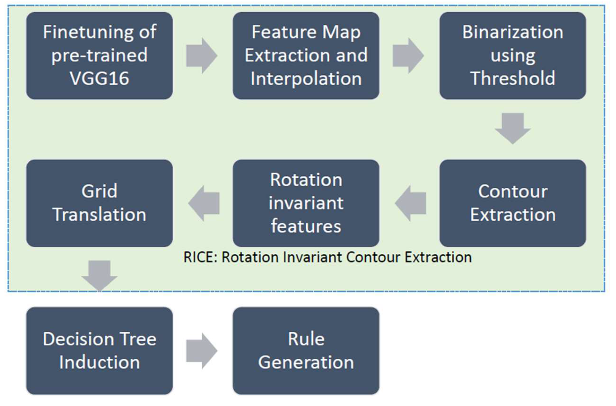
Figure 2.
Source image for sample 6 within Male group.

Figure 3.
Superposed image for feature maps 106 and 423.
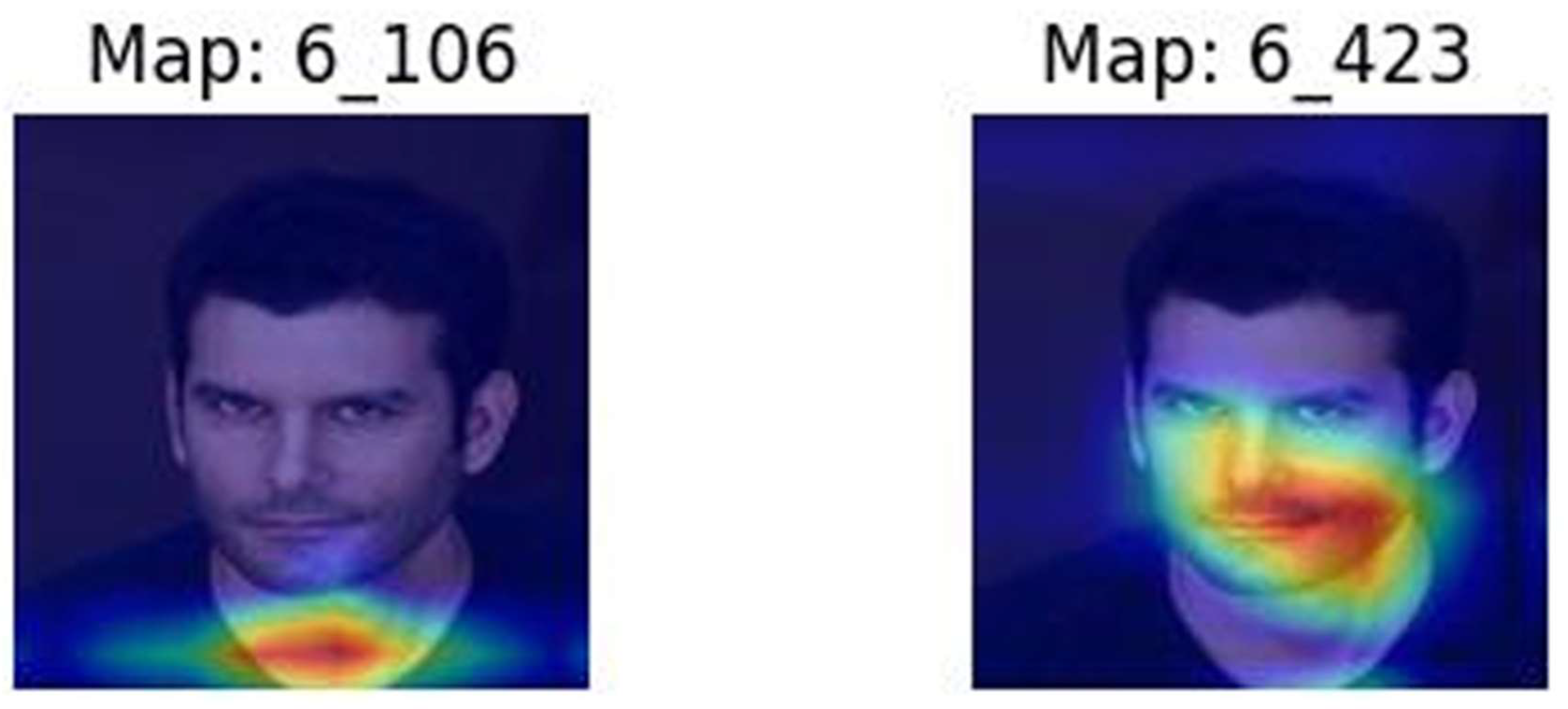
Figure 4.
Source image for sample 6 within the Female group.
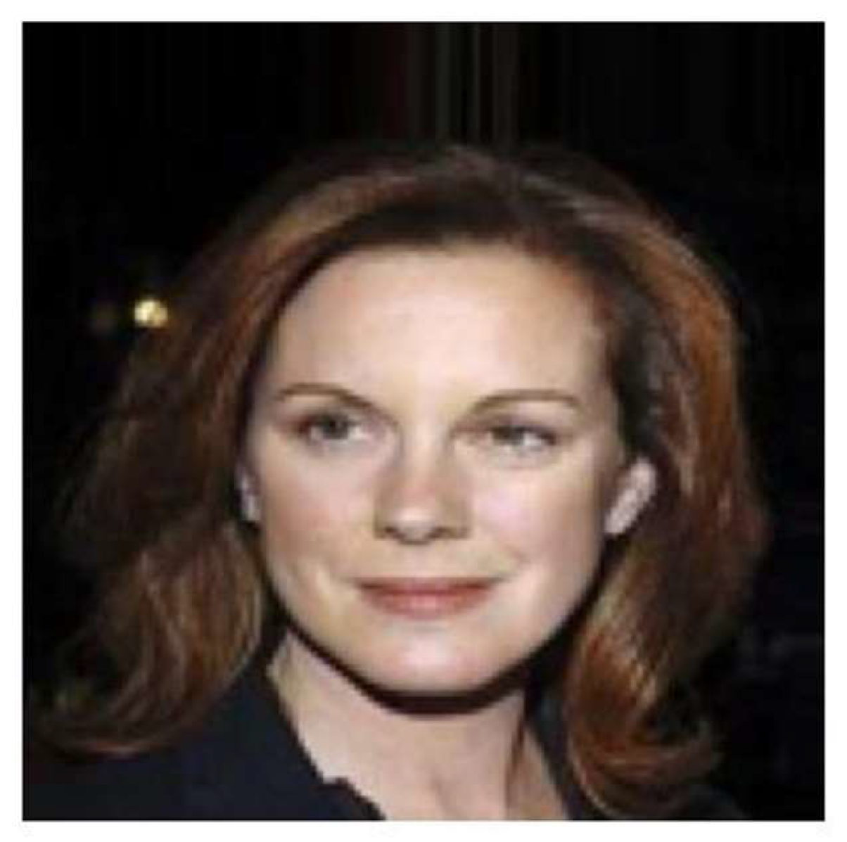
Figure 5.
Superposed image for feature maps 106 and 423.
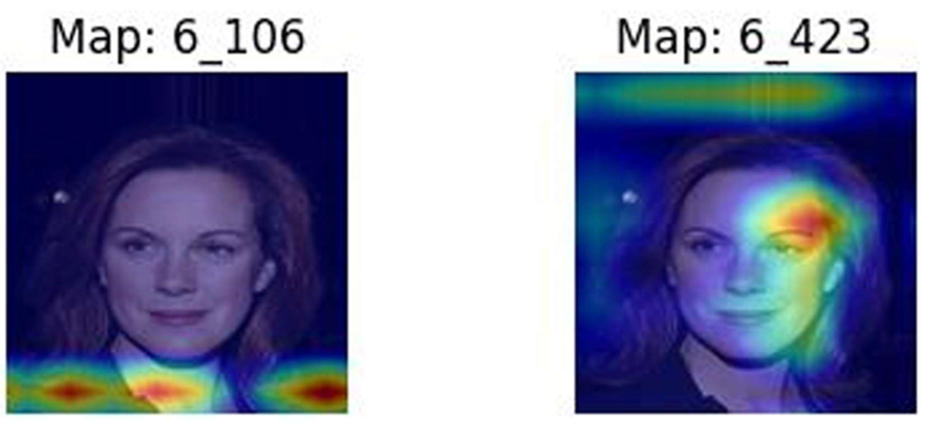
Figure 6.
Partitioning of contour to 2 × 2 grids G1, G2, G3 and G4 numbered left to right, up to down.
Figure 6.
Partitioning of contour to 2 × 2 grids G1, G2, G3 and G4 numbered left to right, up to down.
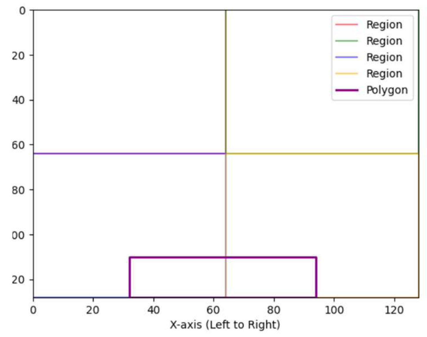
Figure 7.
Decision Tree trained over derived interpretable features and achieving 89.57% Accuracy.
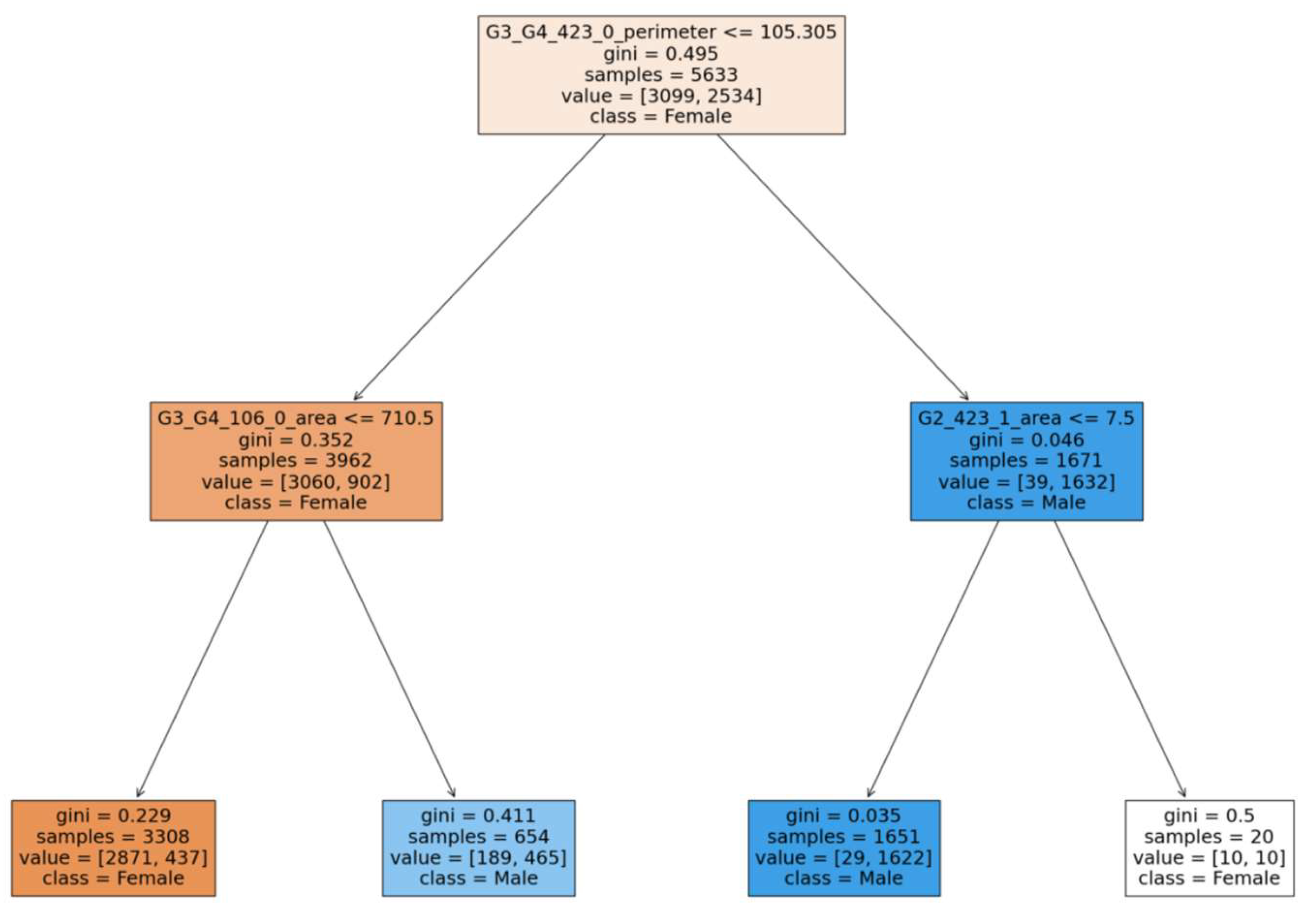
Figure 8.
Eight samples from each class, capturing 2 feature maps and their contours from each image.
Figure 8.
Eight samples from each class, capturing 2 feature maps and their contours from each image.
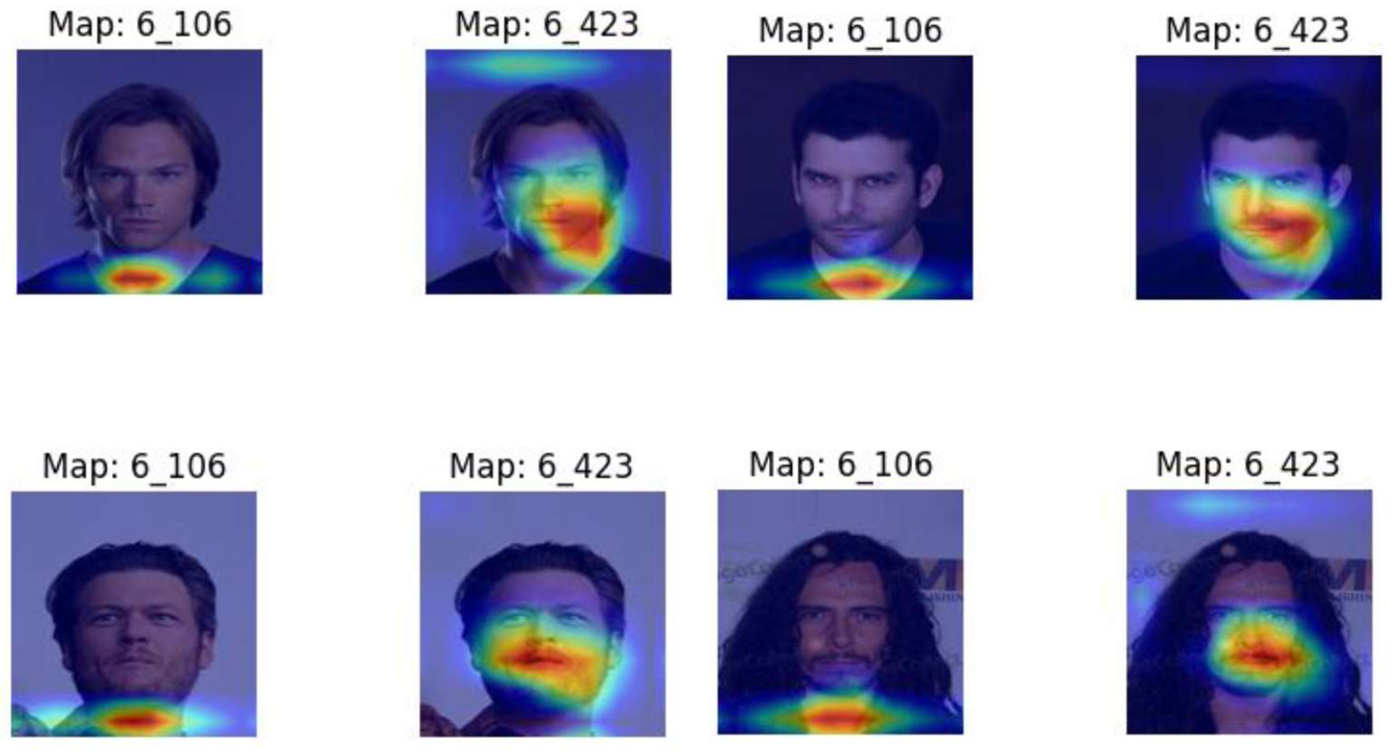
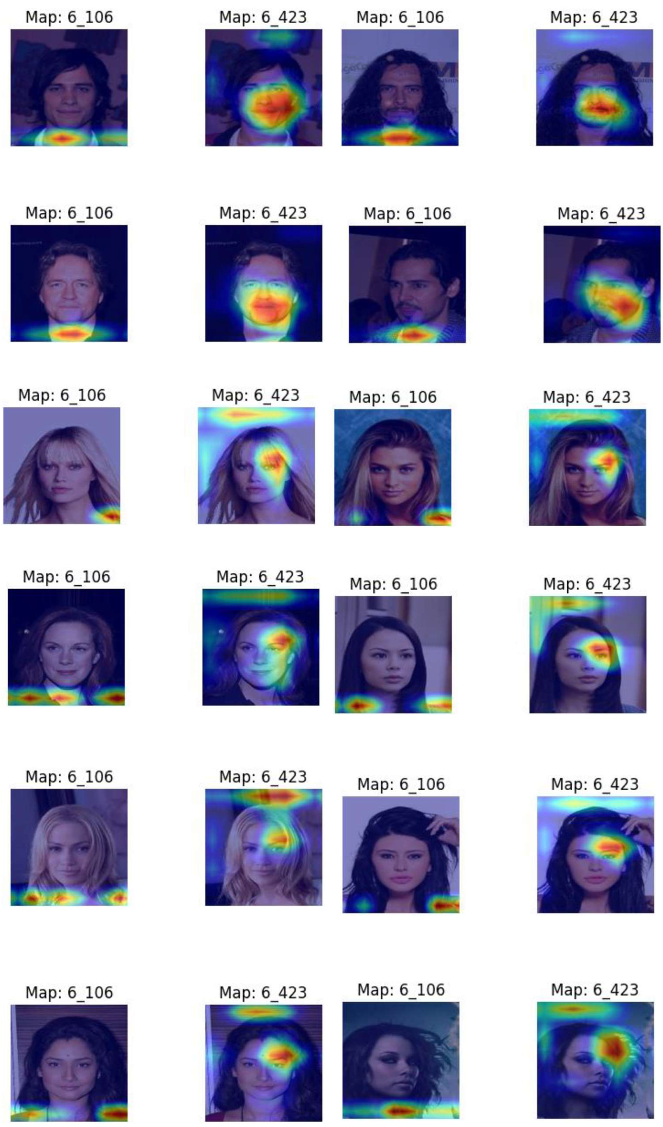
Figure 9.
Sample images from the Dog class.
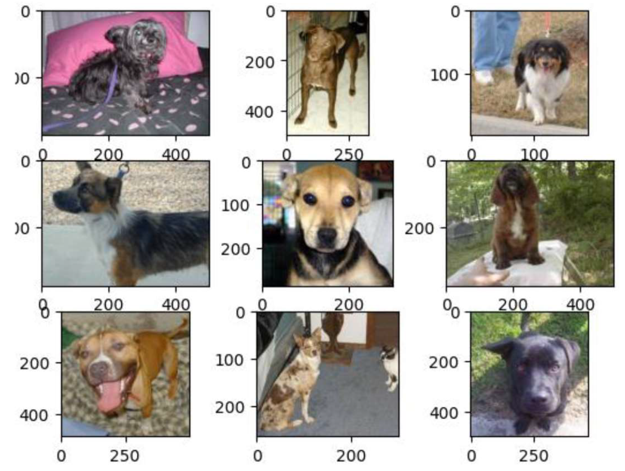
Figure 10.
Sample images from the Dog class.
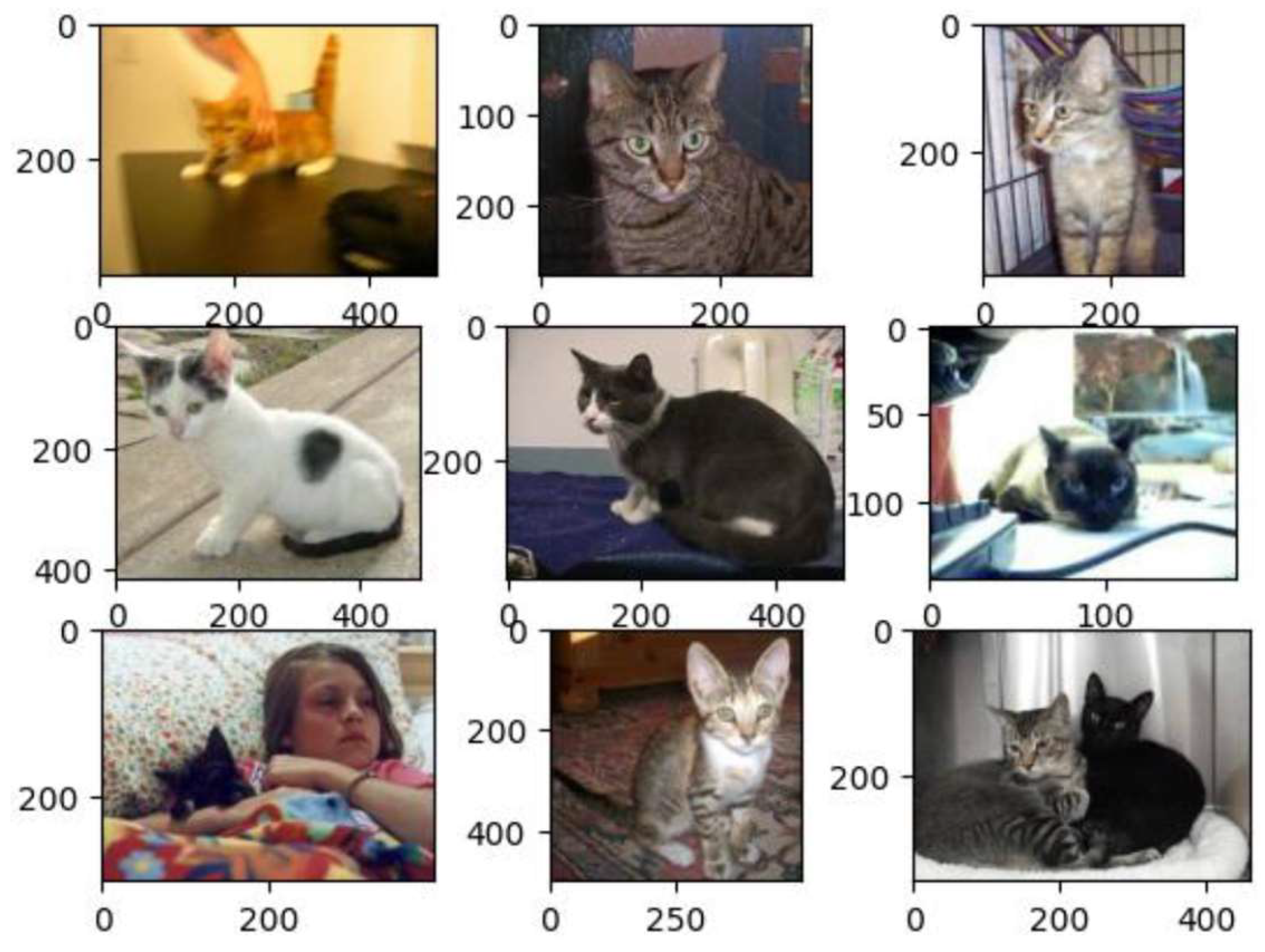
Figure 11.
Samples from the Cat class showing feature Map 6 and its contours.
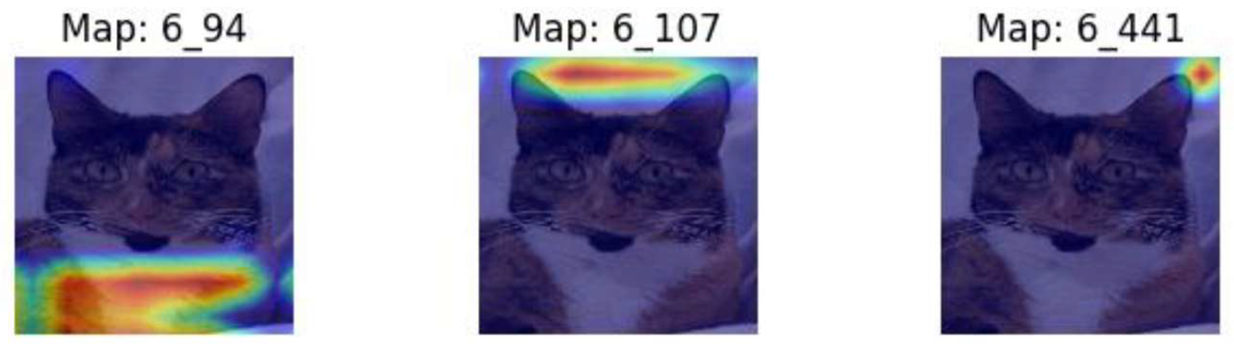
Figure 12.
Samples from the Dog class showing feature Map 6 and its contours.
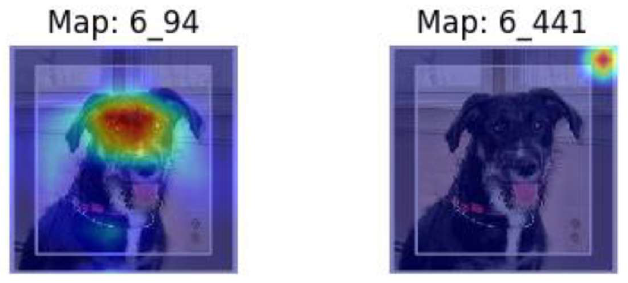
Figure 13.
Decision Tree with depth of 3 trained over derived features, achieving 87.6% Accuracy .
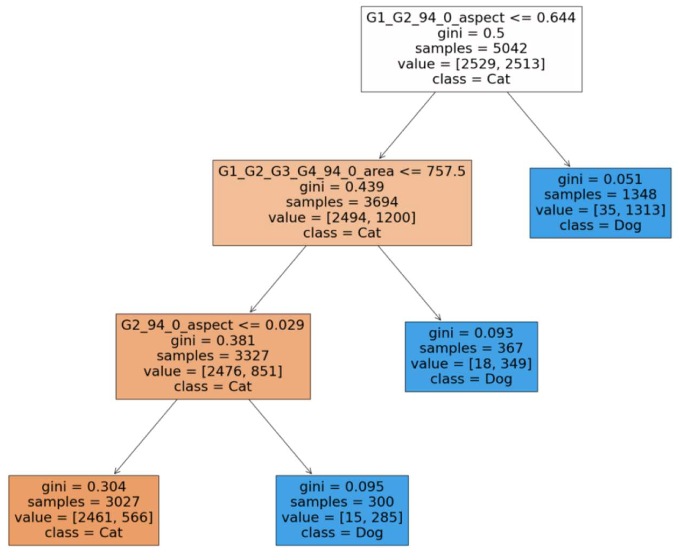

Table 1.
CNN architectural parameters used.
| Parameter | Description and value |
| VGG-16 trainable layers | Last 2 convolutional layers from Block 5 |
| Number of dense layers used | 2 dense layers, 1024 units in layer 1 and 512 in layer 2 |
| Learning rate | .0017 |
| Epochs | 50 |
| Batch size | 512 |
| Early stopping | Yes, with patience value of 6 |
| Optimizer | Adam |
| Input image shape | (128,128,3) |
| Train test validation split | Training and validation partitions used as provided in source for both CelebA and Cats vs& Dogs datasets |
Disclaimer/Publisher’s Note: The statements, opinions and data contained in all publications are solely those of the individual author(s) and contributor(s) and not of MDPI and/or the editor(s). MDPI and/or the editor(s) disclaim responsibility for any injury to people or property resulting from any ideas, methods, instructions or products referred to in the content. |
© 2025 by the authors. Licensee MDPI, Basel, Switzerland. This article is an open access article distributed under the terms and conditions of the Creative Commons Attribution (CC BY) license (http://creativecommons.org/licenses/by/4.0/).
Copyright: This open access article is published under a Creative Commons CC BY 4.0 license, which permit the free download, distribution, and reuse, provided that the author and preprint are cited in any reuse.


