
Submitted:
21 January 2025
Posted:
22 January 2025
You are already at the latest version
Abstract
In this work, we generalize and describe the Golden ratio in the multi-dimensional vec-tor space. We also introduce the concept the law of similarity for multidimensional vectors. Ini-tially, the law of similarity was derived for one-dimensional vectors. Although it operated with such values of the ratio of parts of the whole, it meant linear dimensions (a line is one-dimensionality). The presented concept of the general golden ratio (GGR) for the vectors in the multidimensional space is described in detail with equations and solutions. It shown that the GGR is a function of one or a few angles, which is the solution of equations, or the golden equa-tion, described in this work. Main properties of the GGR are given with illustrative examples. We introduce and discuss the concept of the golden pair of vectors and the set of similarities for a given vector. Also, we present our vision on the theory of the golden ratio for triangles and de-scribe in detail the similarity triangles with illustrative examples.
Keywords:
Golden Ratio
; Generalized Golden Equation
; Set of Similarity Vectors
MSC: 00A30; 11D25
1. Introduction
The golden ratio, or the famous number , is known as the divine proportion between two quantities [1,2]. For positive numbers and , this ratio equals to , if The number was found in proportions of parts in construction of Egyptian pyramids [3], in arts [4]-[6], in fashion [7], in medicine [8,9], face detection [10], image enhancement [11,12], in colors of paintings [13], and many applications in engineering.
In this work we generalize and describe the Golden ratio in the multi-dimensional vector space. We present this concept for the first time, namely, the concept of the general golden ration (GGR) that depends on the direction in the space. Many examples of vectors in golden ratios are described in detail in the 2, 3, and 6-dimensional spaces. Main contribution of this works can be formulated as follows:
- The concept of the golden ratio has generalization in the multi-dimensional space;
- The general golden ratio is function of one or a few angles. It is one of four solutions of the golden equation presented here;
- To each vector in the space corresponds a set of similarity, or a set of vectors being in golden ratio with ;
- GGR can be used to describe similar figures. As an example, the vector space of triangles is described;
- Each vector affects its environment, stimulating its influence through the imposition of its likeness, or similarities.
- The sets of similarities of vectors can be summed.
The rest of the paper is organized in the following way. Section 2 presents the definition of general golden ratio in the vector space. The main equation of the GGR and its solutions are described in Section 3. The golden ratio in the 2D space with examples is considered in Section 4. In Section 5, the concept of the vector similarity sets is presented and described, with examples in the 2D and 3D spaces. The vector space of triangles and golden ratio of triangles are described in detail in Section 6. Illustrative examples are given. In Section 7, similarity figures are described with many examples, including the pentagon, heptagon, the 7 and 9-stars, and Archimedes spiral.
2. The Generalized Golden Ratio (GGR)
In this section, we extend the well-known concept of the gold ratio in the -dimension vector space. Let be the normed vector space over real numbers . It means that exists such a real-valued function , which is denoted by and has the following properties:
- , and means that
- , for any real number
- , for any elements and .
The function is called the length, or the norm, of the element .
Definition 1. In a normed vector space , the function which satisfies the conditions
- , for any elements and
- If
- If
- For any real number , is called the proportion.
As an example, when , the function is the proportion. This is the function that interests us the most.
Definition 2. Given a proportion in the normed vector space , two elements and are called the golden pair, if the following holds:
The elements and are also called the golden ratio elements, or the golden pair.
Definition 3. If the elements and are golden ratio elements, for a proportion then the ratio is called the generalized golden ratio, or shortly GGR.
In the example below for the 1-D vector space, this number is the known golden ratio [1]. Therefore, we use a similar name. In order not in any way to underestimate the historical nature of this number, we added a generalized meaning.
Example 1: Let and the function be the proportion. Here, we consider that for real numbers. To find the golden ratio elements and , we consider the primary equation
It can be written as
or
The solutions of this equation are considered for the following two possible cases.
1. Case : Then, the equation to be solved is
The solutions are
Such numbers are real only when . Therefore,
A golden ratio is a positive number. The first number is considered, but the second is not, since it is negative. Thus, the golden ratio is
2. Case : The following equation is considered:
with the solutions
Such numbers are real only when . Therefore,
Here, is negative and also needs to be discarded, since the condition of consideration is violated, that is, . Thus, a golden pair cannot be composed from numbers of opposite signs. This example shows that for any number there is only one number that composes the golden ratio with . This number is . The golden pair is . In the 1D space , when setting the system of coordinates, we match each point to a certain number, implying by this number some measure of distance from the center of coordinates. Therefore, in the 1D case we deal with linear objects (segments on the real line ) which have the length and it is namely the value for which we obtained a certain proportion called the golden ratio. Two linear objects are in golden ratio, if the ratio of their measures (lengths) is equal to the number .
Now, we will try to move the idea of the golden ratio on the 2D plane (with 1D and 2D objects), considering the starting point 0 in a given system of coordinates. Before we start to work with equations, we need to prepare ourselves to all possible results and ability to explain them. The thing is that 2D objects includes the 1D objects and the golden ratio rule must remain unchanged for them. Let us consider two vectors and the corresponding similar vector (see Figure 1 in part (a)). One can note that the 2D measures of the similar vectors and , or areas of their shadows are in the ratio , not in .
Now we consider that two vectors and are related into one 2D object, the parallelogram, , as shown in part (b). The similar vectors and are also related into another 2D object; the parallelogram . If these vectors are related, then this relation changes; it depends on the angle between these vectors. Then, the question arises how the proportions of these 2D objects cannot depend on connectedness of vectors. In the general case, this number, or the ratio, is the function of the angle, which we denote by When the angle between the vectors is zero, the 2D object is a line. Therefore, in order that the 1D golden ratio can manifest, it is necessary to request the condition . Note that instead of the parallelograms we can also consider other figures, including the triangles composed by these vectors, as shown in part (c). We can call these triangles the golden pair of triangles. Now, we will describe in detail the concept of the golden ratio in a multi-dimensional vector space.
Example 2: Consider the -dimensional vector space It is not difficult to show that the function
is the proportion. Here, the norms and We consider the golden ratio equation (rule) written as
The following calculations are valid for this equation:
Here, is the inner product in the space , and is the angle between the vectors and . Denoting the golden ratio by , we obtain the equation or
This equation has four roots , which are functions of the angle. Thus, the GGR depends on the angle. Since , the roots =, for Also, =.
A. Case (vectors are collinear, or are in the same directions): The equation can be written as
Therefore, we consider the solutions of the equation , which are
The positive solution is Given vector , the golder pair of vectors are in the same direction, and the pair of vectors are in the opposite direction. The second equation has two complex roots,
These complex coefficients of “similarity” are equal to 1 in absolute value, that is, they do not affect the length, but only rotation by . One can say that the first equation in Eq. 8 defines similarity by length and the second equation similiarity by rotation.
As an example, Figure 3 shows the 2D vector at an angle of to the horizontal and four vectors
It is not difficult to see that and These equations hold for any vector .This figure illustrates the concept of similarity of the vector , or similarity by the angle . Among these fours vector, only the first one, is in the golden ratio with .
B. Case (vectors are perpendicular): The equation is reduced to two equations
Therefore, the first equation is considered and its two solutions are
The positive solution is
C. Case (vectors are collinear in the opposite directions): The equation can be written as
Therefore, we consider the solution of equation , which are (see Eq. 4)
The positive solution is Thus, in the -dimensional space, when , two vectors in the opposite directions can compose a golden pair.
D. Case when the golden pair of vectors have the same length, that is Then, Eq. 7 is and the angles . Two pairs of vectors with the angles and 120 (in degrees) between them compose golden pairs when their lengths are equal. Figure 4 shows three vectors and with the same length. Each of these vectors is in the golden ratio with two others.
3. Main Equation of Golden Ration and Its Analytical Solution
In this section, we describe the positive roots of Eq. 7, where is a function of the angle The equation is
with the initial condition =1.61803398. For each angle α, the quartic polynomial in this equation has four roots, and two of them are complex and therefore complex conjugate. We are looking for a positive solution of this equation, which should be only one. Equation 10 can be written as The parabola crosses the straight line with the slope at two points. As illustration, Figure 5 shows the graph of the polynomial together with the line , when in part (a) and in part (b).
For the angle , the solutions of Eq. 10 are
The numbers are written here with 4 decimal precision. At points and , the parabola crosses the straight line , as shown in part (a). The second coordinate is positive. Thus, the required root . For the angle , the solutions of Eq. 10 are
The parabola P(x) crosses the straight line at the point and the positive point . Therefore, 638778… .
The case with the angle (when …) is shown in Figure 5 in part (c). Here, two lines are also shown (in red) as the border lines for the lines , when One can see that all these lines intersect the parabola at two points, one of which is positive and other one is negative.
3.1. Similarity Equation and Its Roots
Consider again the main equation of the gold ratio
We call the continuous roots of this equation the similarity functions and denote them by the symbols . The analytical exact solution of this quartic equation is very complicated [12-15]. The standard procedure is to add an auxiliary parameter to the quartic equation , write it as
and then to request for a square polynomial in square brackets to be a square, that is,
To have such a multiple root , the discriminant of the equation must be zero,
Then, and the above quartic equation can be written as
and solved by two quadratic equations
Cubic Eq. 13 can be reduced to the following depressed cubic equation:
by changing the variable, , as . The Cardano’s solution for this equation states that it has a real root, if the following function is positive:
Figure 6 shows the graph of this polynomial, in part (a); it is positive. Therefore, the solution of Eq. 16 is
The graph of this function is shown in part (b). The function can be used for solving Eq. 14, which will give us four solutions . One can see that the solution formulas of the gold equation are cumbersome and difficult to visualize. Therefore, we now consider another approach, to describe the solutions, by using simple computer programs.
To analyze the equation of the generalized golden ratio, we compute its roots. Figure 7 shows the graphs of four roots , , of Eq. 7. The real and imaginary parts of the roots are shown in blue and red colors, respectively. The angles are in the interval with step 0.0015 radians, or 1/12 degrees. These roots were calculated with the command ‘x=roots([1,0,-1,-2∗cos(a),-1])’, by using MATLAB function ‘roots.m.’
The graphs of the roots are symmetric with respect to the vertical at angle-point . In some parts these functions change sign. For example, the change of sign in the real part of the first solution occurs at angles and and the jump is equals to For other roots, the discontinuities can be seen at angle-points and . As shown in Eqs. 11-17 (see also Figure 6), the analytical solutions (not the ones modeled above) should not have points of discontinuity.
In Figure 8, these four roots are plot in the polar form. The first plot is like the apple, the 2nd as a four-petal flower, the 3rd as the egg (Earth), and the 4th plot is an unknown figure for us.
It is not difficult to note that the following holds for the roots of the above equation: Thus, equals to the sum of the first three roots with sign minus. The 4th plot is the sum in polar form. Figure 9 shows the polar plots of the sum of roots , and in the polar form in parts (a), (b), and (c), respectively. These figures are interesting.
3.2. Analyze of Solutions
It is not difficult to note from Figure 7 that, for each angle, there are two real solutions of Eq. 10. Even more, there is only one positive solution for each angle (see also Figure 5(c)). We will regroup the obtained set of roots , and of the above equation in the following way. The corresponding codes for these four roots are given in Appendix.
For each angle , the first two roots are real and the next two roots are complex conjugate. Then, the solutions are composed as follows:
Figure 11 shows these two roots (solutions) in part (a) The functions and are continuous. The first function is positive and the second one is negative. Both functions are periodic; the period is . It is interesting to note that In part (b), the graph of the sum of these solutions is shown, . The magnitude of this function .
Figure 10.
(a) Two real solutions of Eq. 10 and (b) their sum.
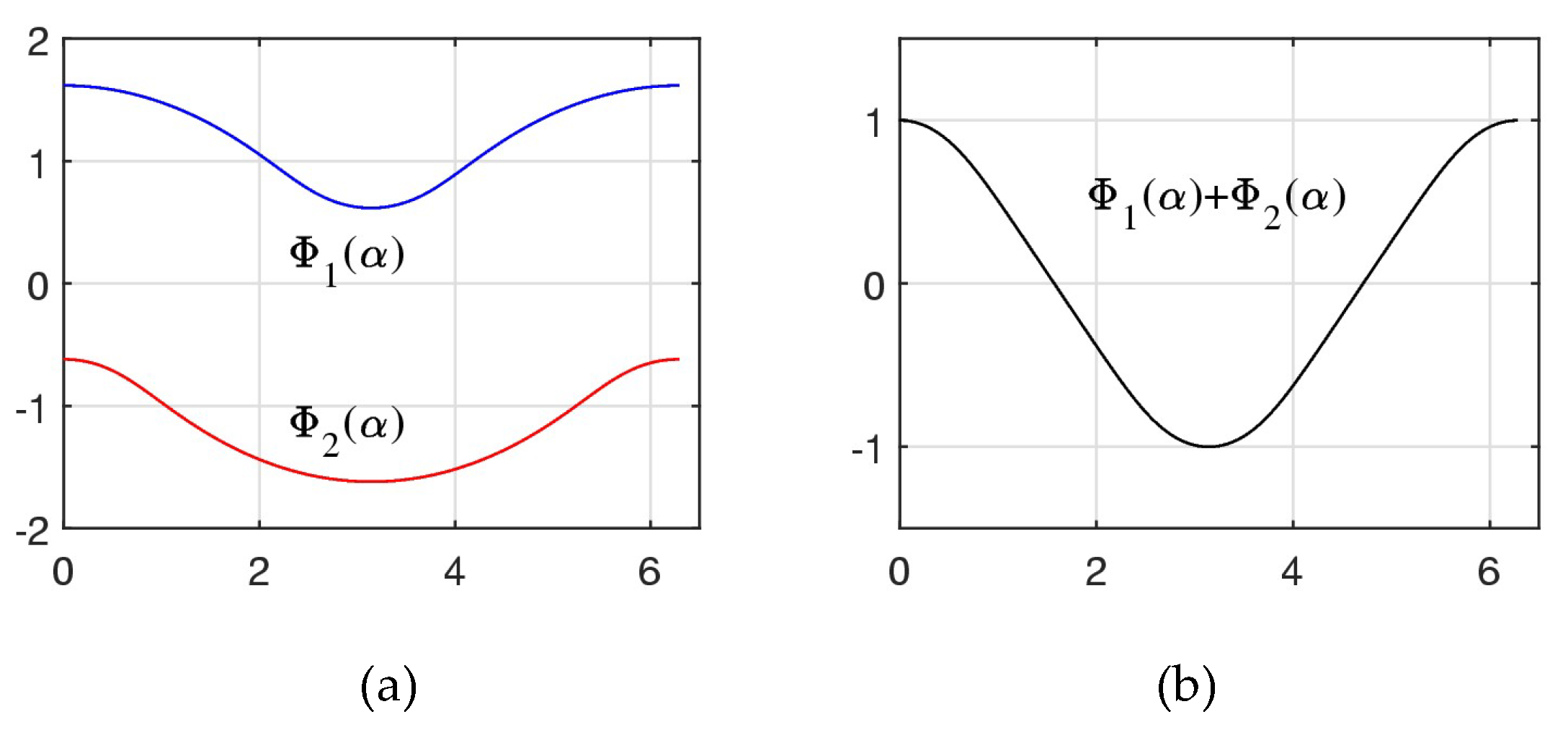
It is interesting to note that the graph of in Figure 10 in part (b) is similar to, but not exactly, the cosine function. This sum of two roots together with the cosine function are shown in Figure 11 in part (a). The difference of these functions is given in part (b). The maximum difference of these two functions is 0.0344590758 (the functions were calculated for angles in the interval .
Figure 12 shows the graph of the positive roots calculated in the interval of interval . We call the function with this graph the general golden ratio function, or the GGR function. For this function, the minimum is 0.6180 at the angle-point , and the maximum is 1.6180 at and . The Golden ratio function equals to 1 at angles and . The mean of the Golden ratio in this interval equals to 1.192880, approximately at angles 1.7385 and 4.5447 in radians, or and .
The GGR function has approximately the form similar to the cosine function. Together with the GGR function, the following function is shown in Figure 13:
Figure 14 shows the graph of the GGR function versus angles in degrees in the interval . A few points on the graph are marked for the values of this function at angles and plus the angle at which the Golden ratio equals to
The complex roots of Eq. 10 can also be regrouped, by using the phases of two complex solutions and Namely, the following functions are calculated:
Note that. MATLAB-based codes for these functions are given in Appendix.
Figure 15 shows the graphs of the real and imaginary parts of the complex solution in parts (a) and (b), respectively. One can note that the real part of the solution has values in the interval Absolute value of this function together with the function is shown in part (c). Here, The function can be considered as an approximation of
3.3. Properties of the Roots
The following properties hold for the roots of the golden equation:
Also, from Eq. 7, we obtain the following identities:
Due to Eqs. 23 and 24, the real part of the 3rd solution (shown in Figure 15) equals to (see Figure 10(b)). It is also not difficult to see that these solutions are transformed into each other under the transformation . Indeed, the following identities are valid, for any angle :
Thus, for each angle , the real ratios can be in two states as . This vector state changes with operator as The full 4D vector of states changes as
4. Examples of Golden Ratios
In this section, we consider a few examples of golden pair of vectors in the 1D and 2D vector spaces.
Example 3 (1D vectors):
For 1D vectors (real numbers), or the elements of the real line , we define the inner product as . Then, the angle is defined as
which means that the angle between similar elements may take only two values, 0 and π. Therefore, the set of similarity, that is, the set of numbers that are in golden ratios with the number is defined as
When that is, the number is in golden ratio with numbers of the set
When that is, , the golden pairs are defined by the similar set
These two sets are equal up to the sign. Here,
Note that and . Thus, for number >0, the set of similarities equals to
For the unit vector , the set of similarities is The golden pairs are and
Example 4 (2D vectors):
Consider two vectors and in the 2D real space . The inner product is defined as and the norm of the vector equals to . All unit vectors have tips on the unit circle, that is, they are described by the set
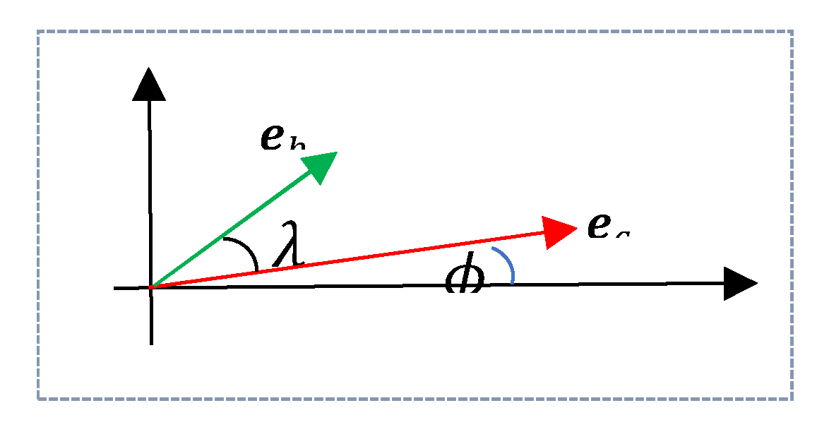
We consider the polar form of the vector and the unit vector at angle to the horizontal (see Figure 17).
Let us assume that the unit vector composes the angle with the vector . The inner product of with the unit vector along the vector equals to
Along the angle , the vector that is in the golden ratio with the vector equals to
Therefore, the set of similarity of the vector is defined as
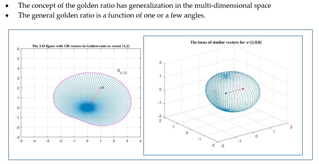
Thus, for a given vector , a golden pair can be found along any direction. The golden ratio changes with angles. As an example, Figure 18 shows the locus of all similarity 2D vectors that compose the golden pairs for the vectors and in parts (a) and (b), respectively. The similarity sets of these vectors are
and
In these figures, the vectors are shown only for 128 uniformly distributed angles from the interval The tips of the vectors are not shown. The figures recall the same petal rotated by different angles and magnifications. The vectors show the orientation of the corresponding sets of similarity .
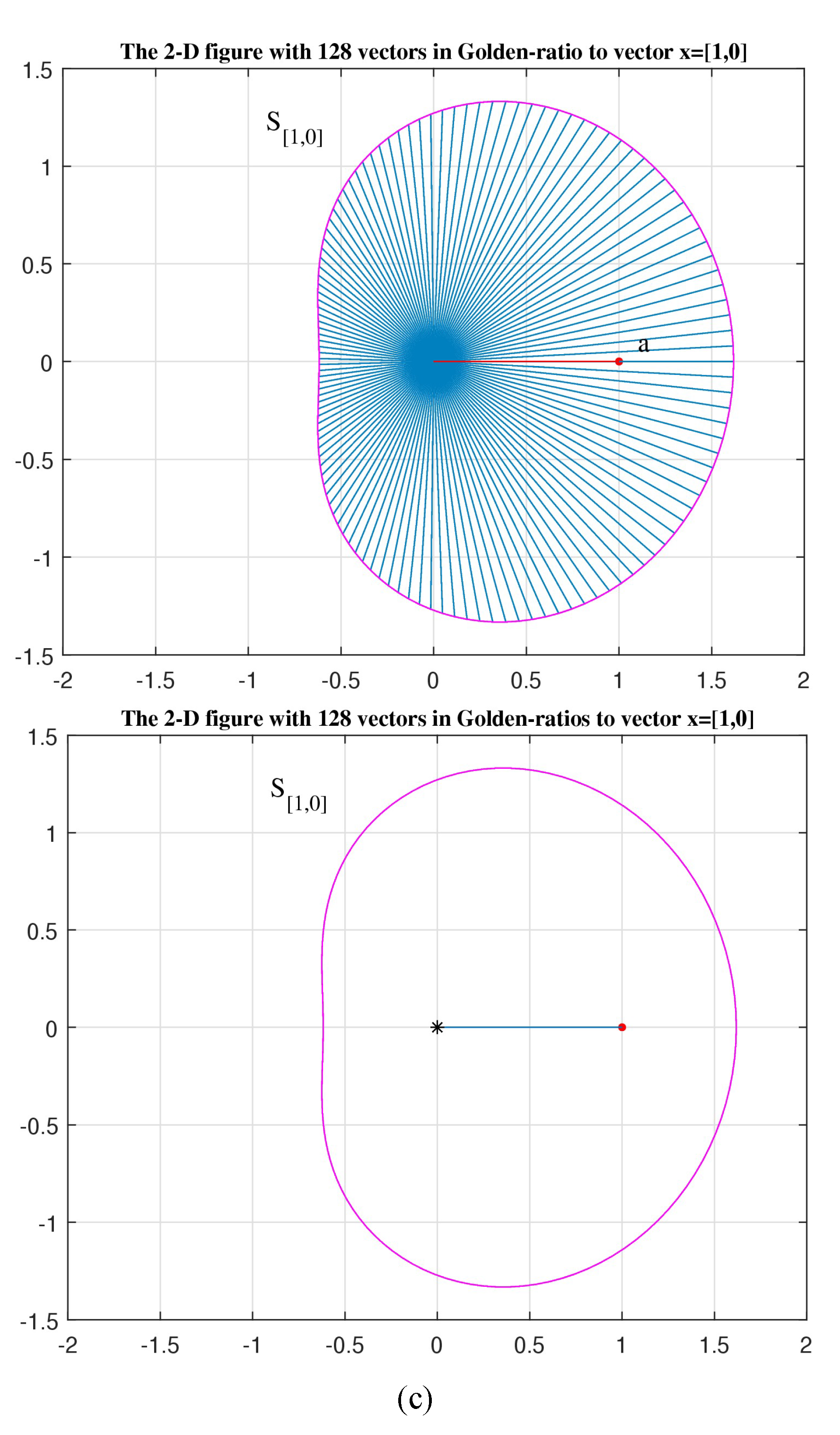
In part (c), the similarity figure is shown for the vector The similarity set of this unit vector is
It should be noted that the figures of the sets of similarity in part (a) and (b) are the rotated figure of part (c) with magnification by the norms and of the vectors and , respectively. The figure for the set can be obtained from the figure of the set by rotation by the angle of and magnified by the number . Similarly, the figure of the similar set in part (b) can be obtained from the figure of by rotation of the angle and magnified by the number .
Figure 18.
(continuation) (c) The locus of 128 Golden pairs with the unit vector
5. Field of Similarities
A. Philosophical digression: What is similarity in our case? Each vector affects its environment, stimulating its influence through the imposition of its likeness. The vector may represent a force, an impulse, or any action in the vector space. If you think about it, then we are all a certain vector of possibilities that we impose on the environment by projecting ourselves into it, and this projection is symbolically represented by a certain projection angle. (All our immediate environment is our projection, our likeness. This is a kind of vector shadow that is cast on the environment, and the ray symbolizes the angle of objectification of this shadow.)
The vector or force in its action can be expressed (presented) by one of its similarity vectors (or forces), in any direction. All these possible similarities, or states of vectors, do not describe the ideal unit circle in 2D case, for one qubit, and the unit sphere in 3D space for two qubits, as assumed in the quantum computing [16]. Here, we have the figure of a petal in the 2D case (Figure 18) and an apple in the 3D case (as shown in the next section).
B. Until now, we knew that if two vectors do not interact and the inner product is zero (that is, the angle is 90 degrees), then mutual influence is excluded. But what is interesting is that the similarity coefficient at this angle is not equal to zero! That is, the influence is still there. According to the printout, it appears that
C. Two roots of Eq. 10 are real, and . The second two are negative. Note that negative numbers do not exist in the nature. We can talk about two, three, etc. objects, which we can not only imagine, but also see (let’s say, 2, 2.5, and 3 apples). One cannot say that about negative numbers, only the imagination works here (let’s imagine - apples). We can say that being positive or negative number are two states, like heads and tails in the probability theory. After all, it was not for nothing that we got two states, , one refers to positive roots, and the other to negative ones. Two other solutions are complex, and ; they show us the 2D representation (the real solutions determine the 1D representation). Note that in English the words imaginary (for complex numbers) and the image have the same root.
D. (The sum of similarity vectors) The following question arises. Is it possible to add similarity fields? If so, then what exactly does the sum of similarities mean? Let us consider two different vectors and at angles of and to the positive real axis, respectively. The corresponding sets of similarities are
These two sets can be written as
Then, their sum should be defined as the set of similarities
where the angle Let us verify if the following is true:
Here, the summation is angle-wise, that is, the summation of vectors that correspond to the same angle Therefore, this equation can be written as
All vectors have the same coefficient of similarity. Removing the similar term from this equation, we obtain
This equation describes the well-known rule for summing vectors over projections. The following calculations are valid for the right part of this equation:
Here, and Thus, everything is correct in Eqs. 38 and 39.
Figure 19 illustrates this property in part (b), where the parallelogram is the result of the rotation of the original parallelogram in part (a), which is composed for the sum of vectors and .
As examples, Figure 20 illustrates the summation of the similarity sets for the vectors and in part (a) and for the vectors , and for in part (b).
Figure 21 shows the same sum of similarity sets, for three pairs of vectors and . Namely, for the vectors and in part (a), vectors and in part (b), and vectors and in part (c). If we assume the vectors represent forces and generate the similarity fields, then the above figures with the sums of similarity sets (fields) may illustrate the influence of fields on space, for example, attraction and repulsion.
It should be noted that we do not sum the similarity sets over equally directed rays. If we do that, that is, if consider the sum of the similar vectors
for each angle , then, we need to find the vector and angle , such that The solution of the equation
is unknown for us.
Example 5 (3-D vectors): We consider the traditional representation of the 3D unit vectors, namely the set
The geometry of the unit vector is shown in Figure 22.
The inner product of such a unit vector with a vector , where , is calculated by
Thus,
The cosine of the angle between these two vectors is the function of 4 arguments, that is, the angle between the vectors and is the function . The similarity set, that is, the set of all vectors in golden ratios with the vector is
Let be the unit vector Figure 23 shows the locus of vectors being in the Golden ratio with this vector in part (a). In this case, and Therefore, and the set of similiarity is
We also consider the unit vector Then, and . Therefore, and the similar set is
The locus of vectors of this similarity set is shown in part (b). In these two figures, as in the 2D case above, only the ends of the vectors as dots are shown. The angles and were taken with the step in the intervals and , respectively. Figure 24 and Figure 25 show these similar sets by different angles. Namely, by using the azimuth (AZ) of zero degree and vertical elevation (EL) of 90 and 180 degrees, respectively. For this, the MATLAB functions ‘view(2)’ and ‘view(0,180)’ were used.
Figure 26 shows the 3D surface that is made up of the vertices of the vectors of a subset of in part (a). Thus, this is the surface framing the vectors which are similar to the unit vector In part (b), the similarity surface is shown for the unit vector For both surfaces, the angles and were taken with the step in the intervals and , respectively.
6. Similarity Triangles
In this section, we consider triangles as elements of the 6D vector space and introduce the concept of the inner product and norm of triangles. The tringles in golden ratio are described and the similarity sets are presented with examples.
In order to show the similarity of three points () in the form of a triangle on the plane (see Figure 27(a)), we need three 2D vectors, which we denote by and . The vectors , and These coordinate vectors compose the 6-D vector Consider two 6D vectors that correspond to two triangles, and The inner product of these vectors is defined as
The norm of the vector is defined as
The norm when a triangle degenerates into point, that is, when , and this case is not considered.
A unit vector, or a triangle, with norm 1 is defined as
We can zero the first 2D vector and consider the unit vector , for which
with condition that and Such 6D vector corresponds to a triangle with the point at the center of the system of coordinates. Such an example is shown in Figure 27 in part (b).
It is follows from Eq. 48, that
Here, is the angle between 2D vectors and . This equation can be written as
Solutions of this equation can be written as (
Thus, we have a parameterized set of solutions; two parameters are the angles and The solutions can be written as
Here, and This system of solutions connects the lengths and the angle between the sides of the triangle, and . Note that, to generalize this solution, we can add a zero element with norm 0. Indeed, for a 2D vector =1.
The vector can be analytically written as
The angles in Eqs. 51 and 52 are considered the same.
 |
Thus, the vector is parameterized by two angles, that is, In this system, the vector is rotated counter clock-wise by the angle and the vector by the angle (from the horizontal). We denote the set of such unit 6D vectors (triangles) by As examples, Figure 28 shows five unit triangles with the angle . The first triangle with angle is shown in red with vertices marked. Other four unit triangles are shown with the angles and 130
Two other examples with unit triangles are shown in Figure 29. Four unit triangles with angle are shown in part (a), when angles and 100 In part (b), three unit triangles with angle are shown, when angles and .
For a 6D vector presenting a triangle, the similarity triangle, or the triangle in the general golden ratio with , is defined as
Here, ) denotes the angle between vectors and , which is calculated by
The norm is calculated as in Eq. 47 and the inner product is calculated by
As an example, Figure 30 show the triangle described by the vector in part (a). The angle between the vectors and equals to and . The similarity triangles , and for angle , are shown in parts (b), (c), and (d), respectively.
For the vector , the similarity set of triangles is defined as
Also, we can write this set as As example, Figure 31 in part (a) shows the subset of the similarity set , for the vector which represents a right triangle with angle between sides ab and ac (shown in red). The angle is the angle between vectors and . The unit vectors are calculated by Eq. 51 and 52, for 23 angles The second parameter , that is, the angle between the vectors and in the similarity triangles is the same as in the triangle for . In part (b), the subset of another similarity set is shown, for the vector . This vector represents a triangle with angle of between vectors and (shown in red). 26 angles of are used, namely , and the angle
In Figure 32, the similarity subsets are shown for the equilateral triangle with sides of length 5. The corresponding vector is . The first point of the triangle is not at the origin. In part (a), the subset of similarity triangles is shown for 29 angles and angle This is the case when . In part (b), the subset is shown for the same 29 angles of and the angle
What can be seen from the figures above, among similarity triangles there is no equal to the triangle with the vector . It also not difficult to see from Eq. 53, that only if
that is, when , or and It is possible that other definitions of the inner product of triangles could lead to similarities that include the original triangle .
As was mentioned above, to generalize this solution, we can add to unit vectors a zero element with a 2-D vector Therefore in general, we can consider the similarity set of triangles of the vector-triangle as a set parameterized by angles and vector ,
To facilitate understanding, we can separate similarities, by fixing two parameters out of three. Also, we can consider these similarities separately (as spatial similarity, similarity in one fixed angle , or similarity in rotation ). If we are interested in similarities with a fixed angle between two sides, then we should fix the value of λ by giving it the value of one of the angles of the original triangle. Adding a constant vector leads to a spatial shift (translation) of the set of similarities.
7. Similarity of Figures (not Vectors)
The concepts of the similarity vectors and similarity sets of vectors, or golden vectors, are defined in the vector space. These concepts were described in detail and illustrated in Section 6 on examples with triangles represented as vectors. In this section, we present the concept of similarity on figures, not as vectors. In general, it is difficult to describe many figures (objects), for example the 7-pointed star, in the vector space. The generalized golden function can also be used in the simple case for similar figures (or objects), considering the change of the size of a given figure according to this function, as the function of angle, that is, after rotation of the figure. Now we will illustrate this simplified concept of similar figures on examples in the 2D plane, which include the well-known figures, such as the pentagons, heptagons, stars, and spirals.
Example 6: (Triangle)
Let is consider the following three points on the place , and These points together compose one triangle, which we donote by . We need to draw the triangles which are in golden ratio with the triangle but rotated by . Figure 33 shows the original triangle in part (a) (in black color) together with the rotated triangle (in magenta). The solution of the golden equations for this angle are
Two roots are positive, and are positive, and only the first one is positive. The similar triangle, that is, the triangle in the golden ratio, is shown in part (b). The small triangle in part (b) is which is not in the golden ratio with . In part (c), the original triangle is shown in blue and the triangle in the gold ratio with it in green.
The triangles that are in golden ratio with at angles 30, 140, and -20 are shown in Figure 34 in parts (a), (b), and (c), respectively. Note that the system of coordinates is not in the center of the triangle and the golden pairs change the original form (angles) of the triangle.
7.1. Other Figures
Now, we consider a few more illustrative examples for the GGR function in the 2D vector space. The figures of regular polygons and stars are considered with their centers at the initial point of the coordinate system. The form of golden pairs for each of such figures is preserved, as shown below.
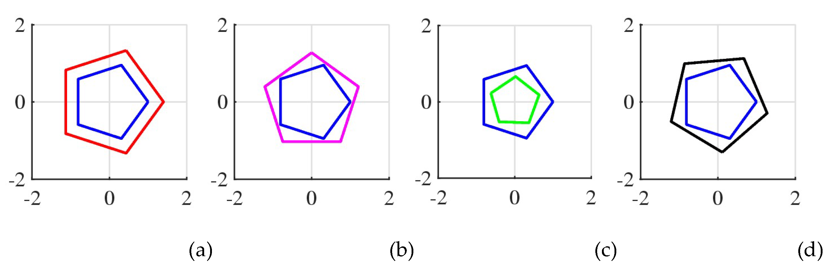
Example 7. Consider the pentagon, , inside the unit circle, which is shown in Figure 34 in the blue color. The hexagons that are in golden ratio with at angles 72, 90, 160, and 275 are shown in parts (a), (b), (c), and (d), respectively.
Figure 34.
The pentagon and its golden pairs for the angles 72,90, 160, and 275.
Example 8. Consider the heptagon, , inside the unit circle, which is shown in Figure 35 in the blue color. The heptagons that are in golden ratio with at angles 30, 140, -100, and 200 are shown in parts (a), (b), (c), and (d), respectively.
Example 9. Consider the 7-pointed star, or the regular heptagram, inside the unit circle. This star is shown in Figure 36 in the blue color. The heptagrams that are in golden ratio with at angles 30, 90, 160, and 220 are shown in parts (a), (b), (c), and (d), respectively.
Example 10. Consider the 9-pointed star, or the regular enneagram, inside the unit circle. This star is shown in Figure 37 in part (a). The enneagrams that are in golden ratio with at angles 90, 160, and 220 are shown in parts (b), (c), and (d), respectively.
Example 11. Consider the figure with the cross, along with 10 crosses of half the size, each arranged in a circle, as shown in Figure 38 in part (a). This is a traditional picture with complete symmetry and identical figures. There is complete symmetry and there is no movement in this picture. In part (b), 10 crosses on the circle are chosen from the golden pairs with angles 18, 54,,, …, and 342. In part (c), the same cross in the center is shown together with 12 its golden pairs for by angles 15,,,, 145, …, and 335.
Example 12. Consider the 5-pointed star together with 12 starts of twice smaller starts which are shown in Figure 39. In part (a), the traditional picture is shown, and in part (b), 12 starts are composing the golden pairs with the star in the center.
Example 13. Consider the 7-pointed star, shown in the center of Figure 40 in part (a) and 12 golden pair-starts placed around a circle. These golden pairs were calculated for star twice smaller size, . Figure 15(b) shows the similar picture for the 9-pointed star, . The golden pairs of stars were calculated for angles 15,,,, 145, …, and 335.
Example 14. Consider the locus of the first 108 points on the Archimedes spiral }. We can call this figure a linear spiral . Figure 41 shows this spiral in the center together with 8 spirals which compose golden pairs with the spiral /2 of twice smaller size. These 8 spirals are placed around a circle with distance of .
If we superimpose these shapes on top of each other, we get a 3D shape. As examples, Figs. 42 shows such 2D view for the -sided polygons , for and 7. The angles were taken from the interval with the step of 2 degree. The original polygons are shown on the x-y plane in the black color.
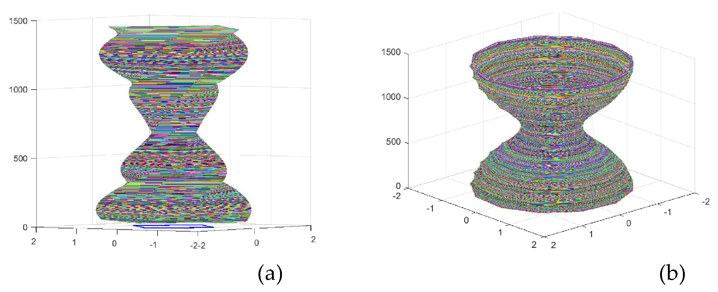
Figure 43 shows such shapes for the square in part (a) and for the twelve-sided polygon (dodecagon) in part (b). In these shapes, the polygons in golden ratios are colored randomly and angles were taken from the interval with the small step, 0.2. These two figures exist in the nature.
8. Afterword and Conclusion
In this work of our research, we generalize the similarity law for multidimensional vectors. Initially, the law of similarity was derived for one-dimensional vectors. Although it operated with such values of the ratio of parts of the whole, it meant linear dimensions (a line is one-dimensionality). Now the question arises - where can one observe this generalization? If we refer to the forms of fruits, for instance the apple, then it is easy to see a strongly pronounced broken sphericity, which does correspond to the listed forms.
The main part of this research is the concept of similarity, namely the set of similarity vectors to a given one. In all graphics above, the vectors were used, not area or surface (in the 3D case). The vector represents the force. This concept is difficult to explain, even to understand. There is a mystery here that we can't solve. Intuitively our subconscious mind shows that a certain vector spreads itself in the surrounding space. What we consider local, as a certain center of outflow of a narrowly directing force, is an abstraction. Any force retains its likeness around itself and has spatial dimensions even in the opposite direction. Physically, it's hard to imagine. Psychologically, it can be imagined in the following way. If you accompany the realization of force, then you will have a gain (), but your opposition to it is not completely destroyed (). Nature reserves the right to object with coefficient , when there is a right to encourage with coefficient . Also, , which means that the impact of the external environment is intended only to separate those who are with it from those who are against it. Deviations of action along all other angles between standing and confrontation tend to roll to one of these sides (the sign of the derivative of ). In this perspective, the law of similarity is clear.
Author Contributions
Conceptualization, A.G. and M.G.; methodology, A.G. and M.G.; software, A.G. and M.G.; validation, A.G.; formal analysis, A.G. and M.G.; investigation, A.G. and M.G.; resources, A.G.; data curation, A.G.; writing—original draft preparation, A.G. and M.G..; writing—review and editing, A.G.; visualization, A.G. and M.G.; supervision, A.G.; project administration, A.G. All authors have read and agreed to the published version of the manuscript.
Funding
This research received no external funding.
Institutional Review Board Statement
Not applicable.
Data Availability Statement
The main codes are given in Appendix; other codes will be available on the web page https://ceid.utsa.edu/agrigoryan/codes/
Conflicts of Interest
The authors declare no conflicts of interest.
Appendix A
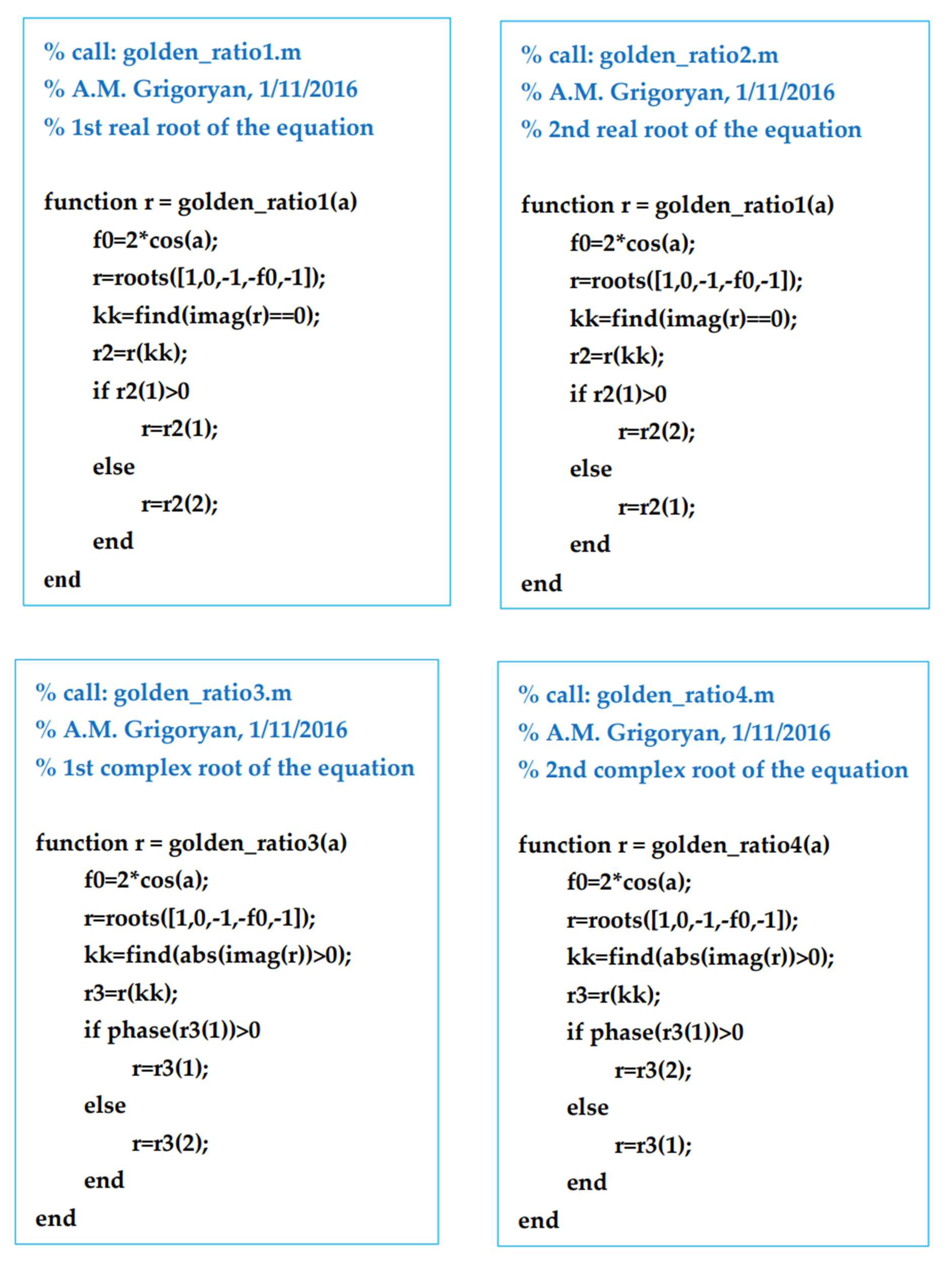
The MATLAB-based codes for computing the solutions of the golden equation are given below. The following functions are used to compute these solutions:
- 1)
- golden_ratio1.m (for , given an angle ),
- 2)
- golden_ratio2.m (for , given an angle ),
- 3)
- golden_ratio3.m (for , given an angle ),
- 4)
- golden_ratio4.m (for , given an angle ).
References
- Stakhov, A. The golden section and modern harmony mathematics, in book: Applications of Fibonacci Numbers, Springer Netherlands, 1998, 7, 393-399,.
- Bradley, S. A geometric connection between generalized Fibonacci sequences and nearly golden sections, The Fibonacci Quarterly, 1999, 38:2, 174–180.
- Herz-Fischler, R. The Shape of the Great Pyramid, Wilfrid Laurier University Press, 2000.
- van Zanten, A. The golden ratio in the arts of painting, building and mathematic, Nieuw Arch. Wisk., 1999, 17:2, 229–245.
- Olariu, A. Golden section and the art of painting, National Institute for Physics and Nuclear Engineering, 1999, 1–4.
- Grigoryan, A.M.; Agaian, S.S. Evidence of golden and aesthetic proportions in colors of paintings of the prominent artists, IEEE MultiMedia, Jan.-March 2020, 27:1, 8-16. [CrossRef]
- Kazlacheva, Z.; Ilieva, J. The golden and Fibonacci geometry in fashion and textile design, Proc. of the eRA, 2016, 10, 15–64.
- Chan, J.Y.; Chang, G.H. The golden ratio optimizes cardiomelic form and function, Journal of Medical Hypotheses and Ideas, 2009, 3, 1-5.
- Henein, M.Y.; Collaborators, G.R. etc. The human heart: application of the golden ratio and angle, International Journal Cardiology, 2011, 150(3), 239-242.
- Hassaballah, M.; Murakami, K.; Ido, S. Face detection evaluation: a new approach based on the golden ratio, Signal, Image and Video Processing, 2013, 7:2, 307–316.
- Grigoryan, A.M.; Agaian, S.S. Monotonic sequences for image enhancement and segmentation, Digital Signal Processing, June 2015, 41, 70–89. [CrossRef]
- Federica, L.N; Barry, M. Reading Bombelli, The Mathematical Intelligencer, 2002, 24:1, 12–21. [CrossRef]
- Victor K. A History of Mathematics. Boston: Addison Wesley, 2004, p. 220.
- Nickalls, R.W.D. Viète, Descartes, and the cubic equation, Mathematical Gazette, July 2006, 90:518, 203–208.
- Press, W. H.; Teukolsky, S.A.; Vetterling, W.T.; Flannery, B.P. Section 5.6 Quadratic and Cubic Equations, Numerical Recipes: The Art of Scientific Computing (3rd ed.), New York: Cambridge University Press, 2007.
- Nielsen. M.; Chuang I. Quantum Computation and Quantum Information, 2nd Ed., Cambridge UP, 2001.
Figure 1.
(a) The golden pair of vectors and these vectors with (b) the parallelograms and (c) triangles.
Figure 1.
(a) The golden pair of vectors and these vectors with (b) the parallelograms and (c) triangles.
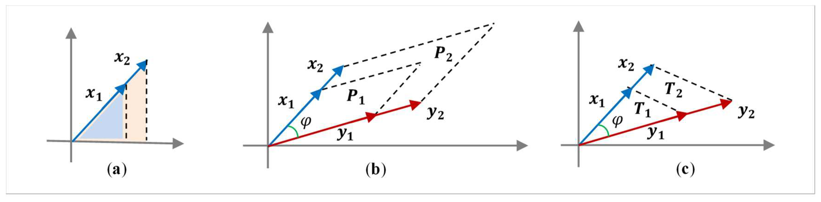
Figure 3.
The vector and its four similarity vectors.
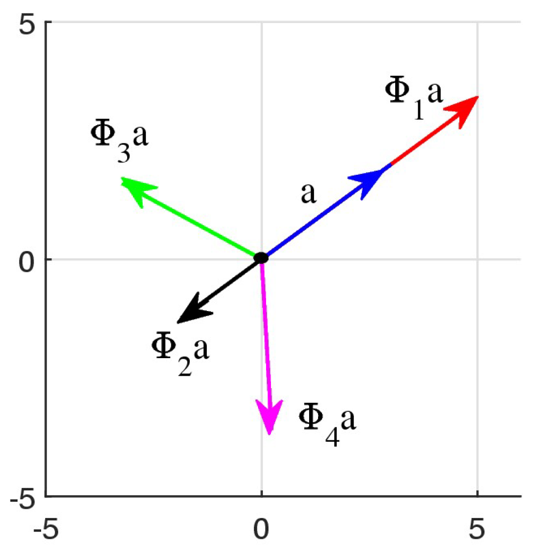
Figure 4.
The golden pairs , and
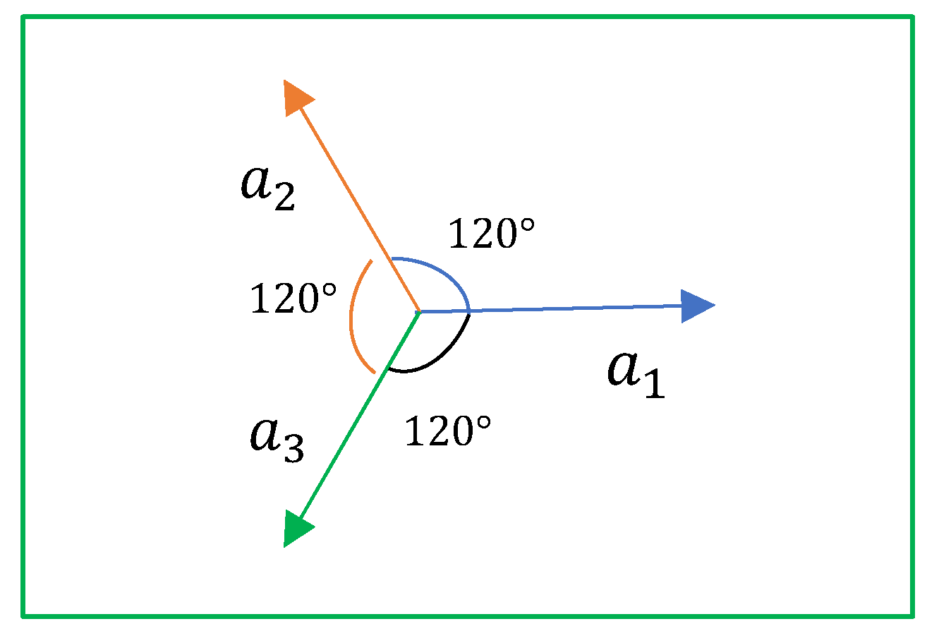
Figure 5.
The graphs of the polynomial and lines, when (a) , (b) , and (b) .
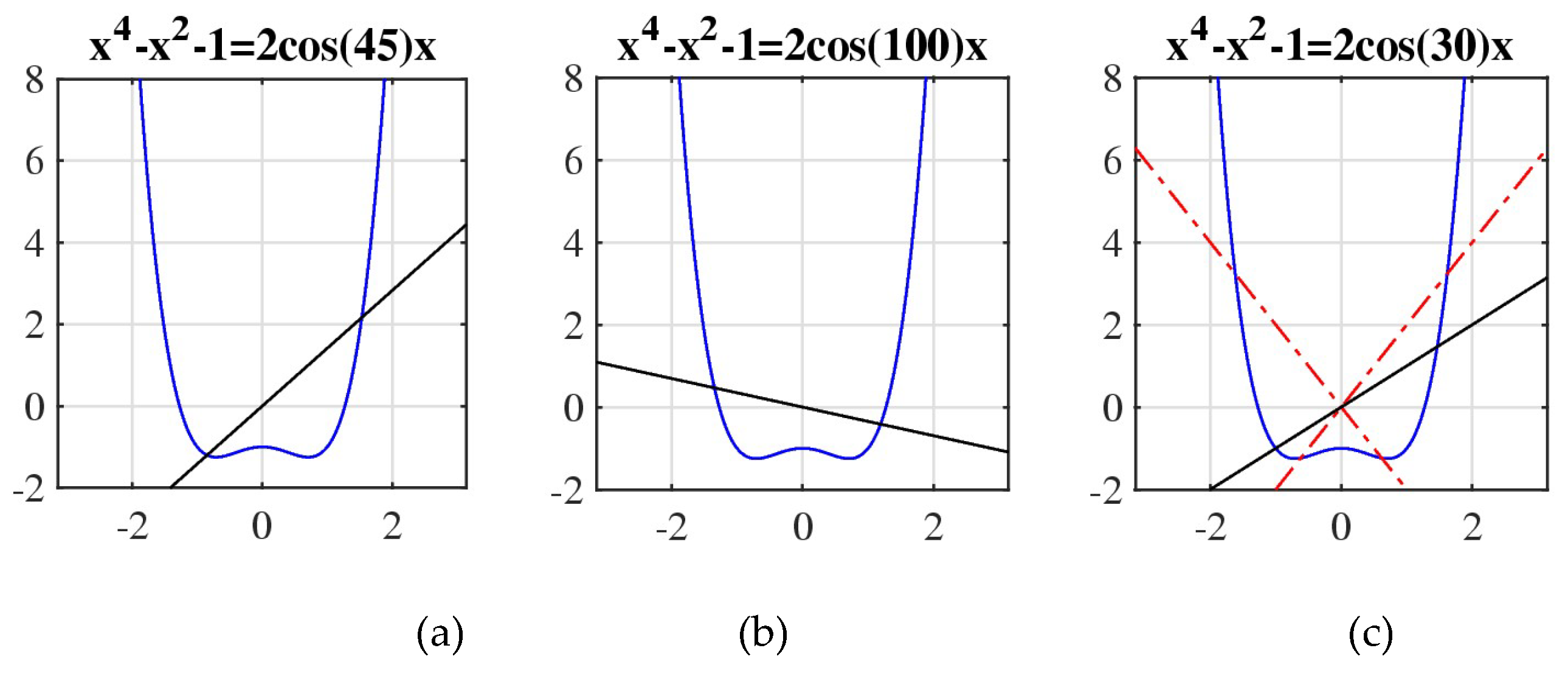
Figure 6.
The positive functions (a) and (b) for the Cardano’s solution of the depressed equation.
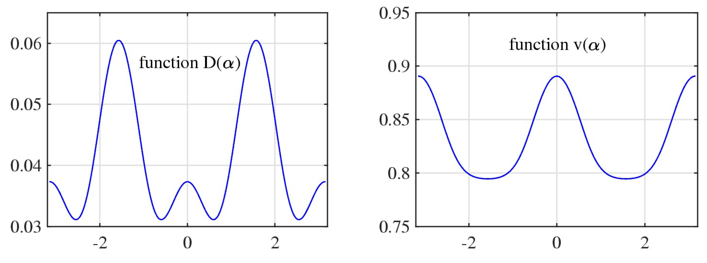
Figure 7.
The graphs of the four roots of Eq. 10.
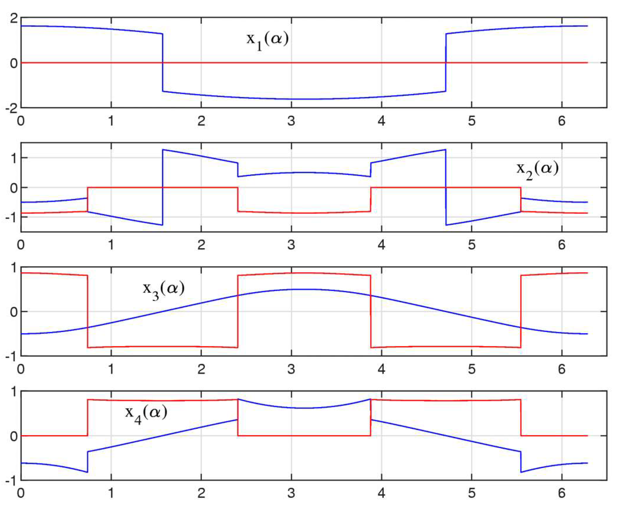
Figure 8.
Polar plots of magnitudes of four roots of Eq. 10.
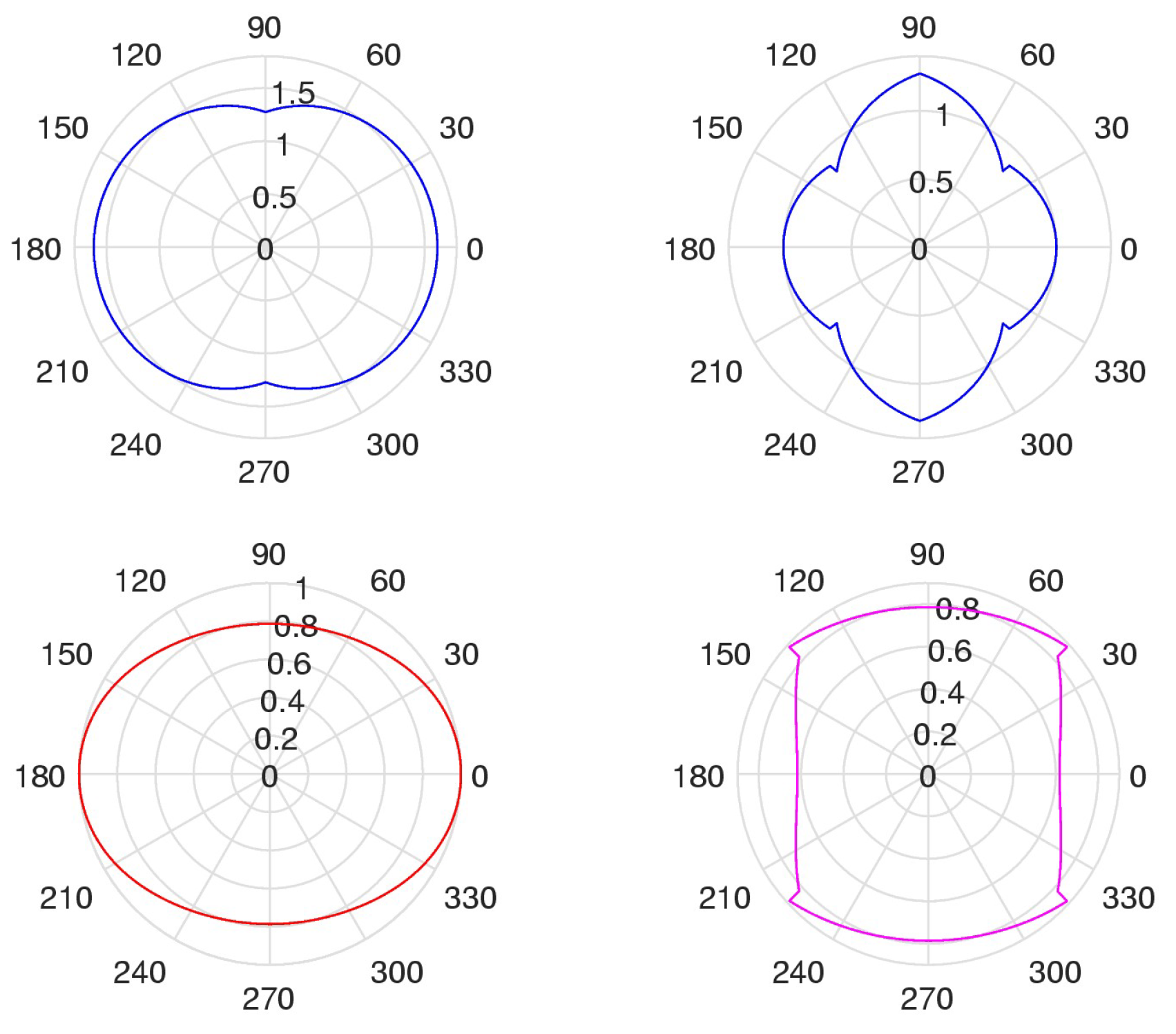
Figure 9.
The polar plots of the sum of two roots: (a) , (b) , and (c) .
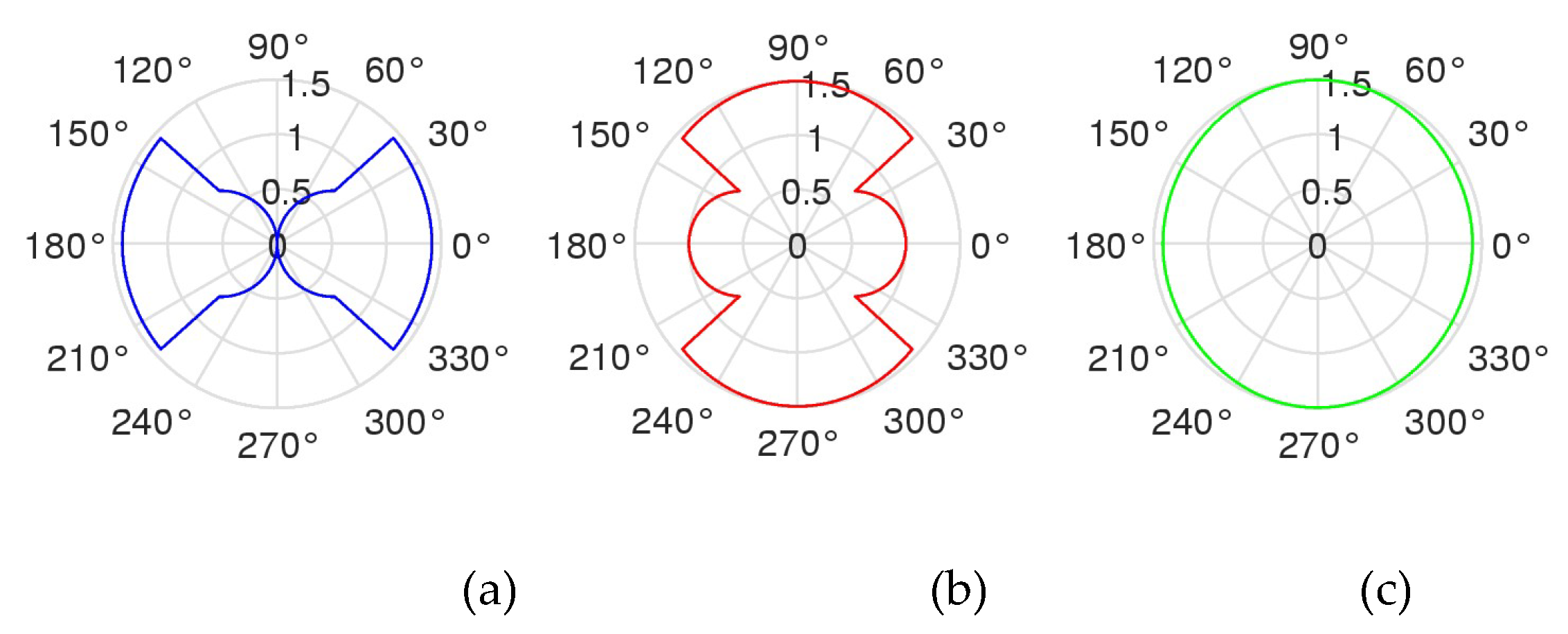
Figure 11.
(a) The sum of real solutions and the cosine function and (b) their difference.
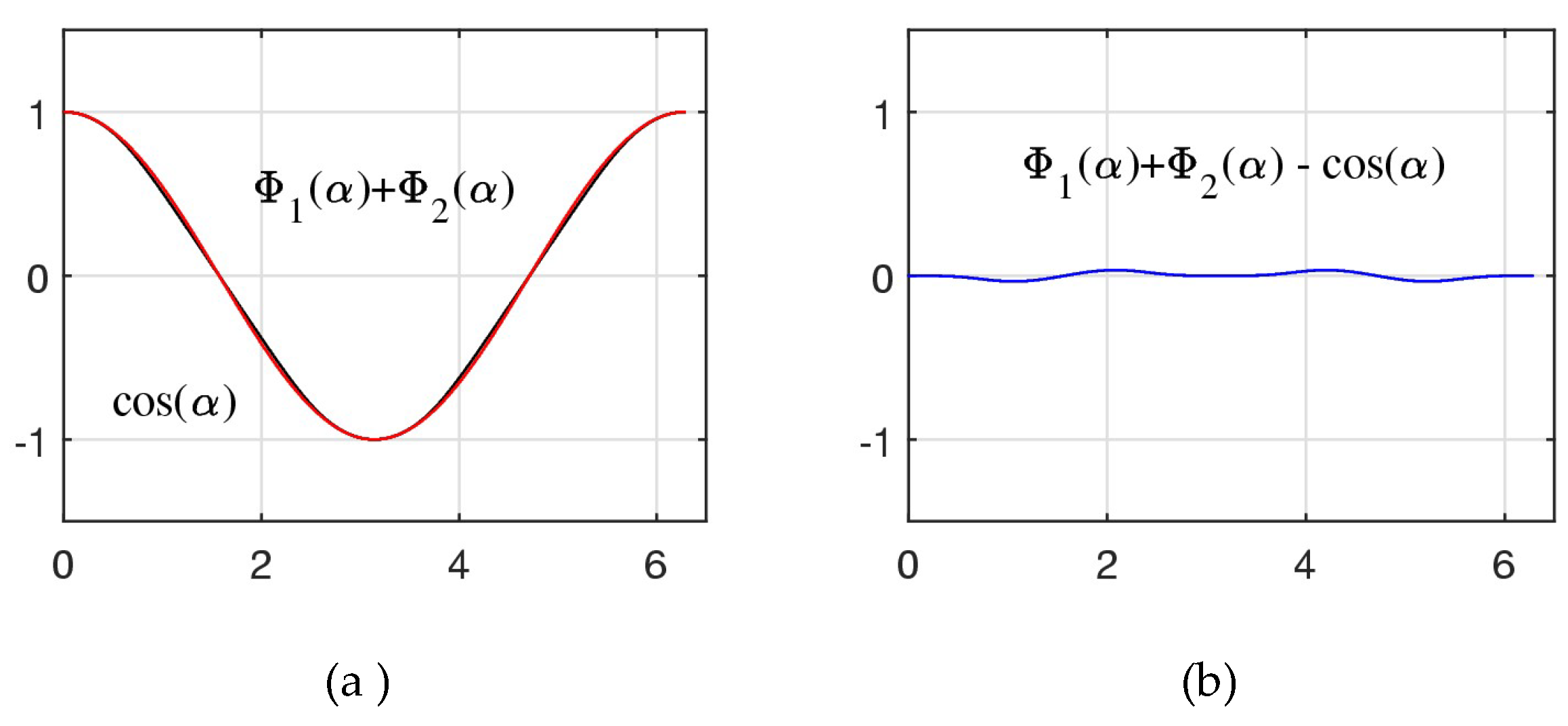
Figure 12.
The general golden ratio function .
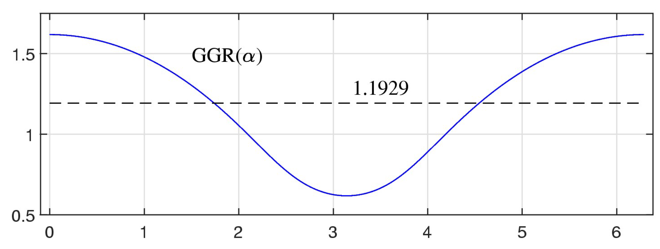
Figure 13.
The general golden ratio function and the function .
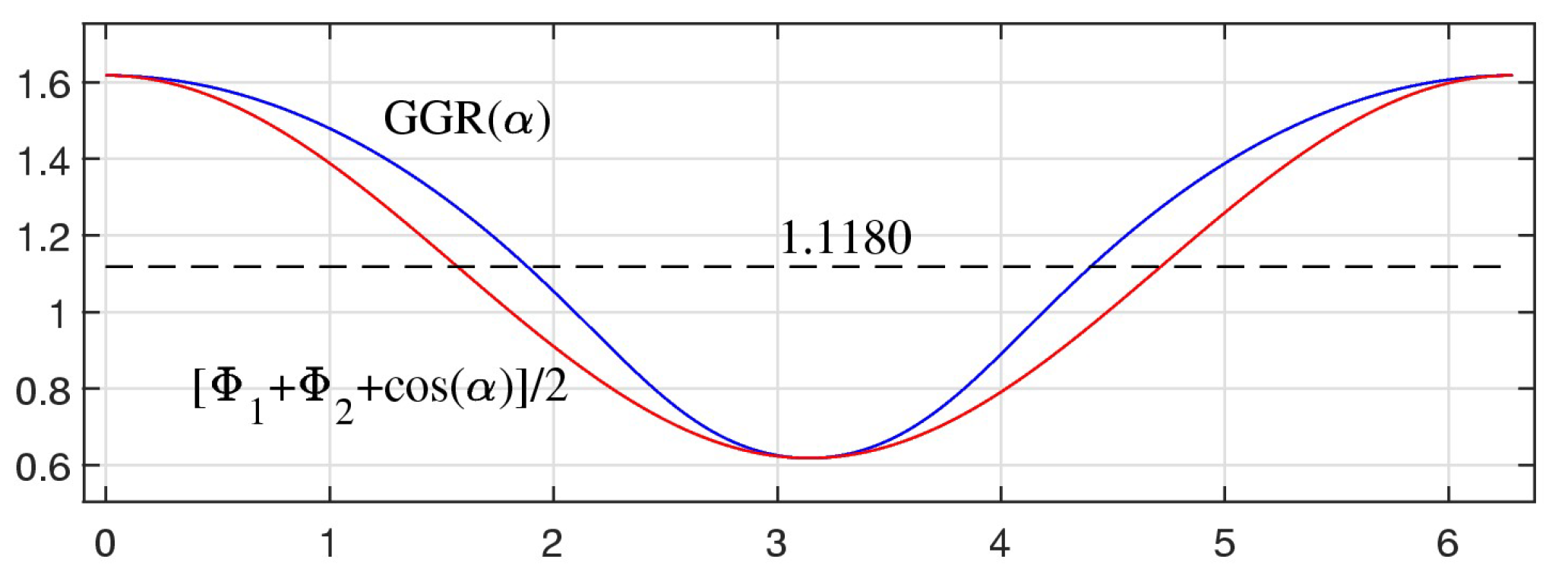
Figure 14.
The General Golden ratio function with a few marked values on it.
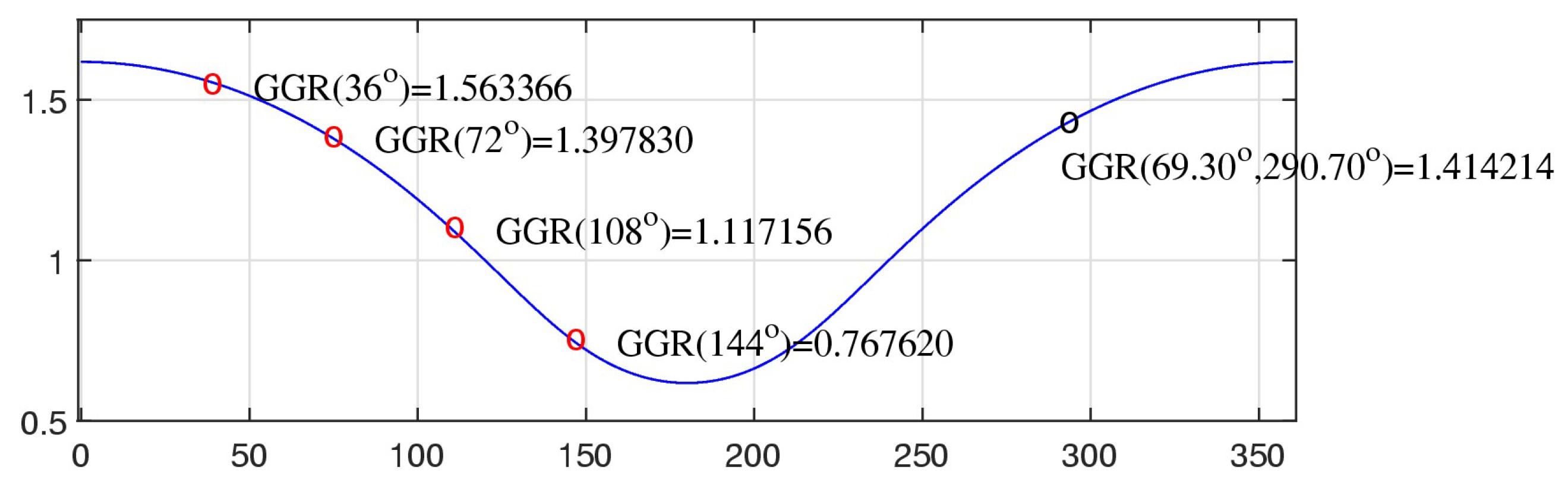
Figure 15.
The complex solution : (a) the real part, (b) the imaginary part, and (c) the magnitude and its approximation . .
Figure 15.
The complex solution : (a) the real part, (b) the imaginary part, and (c) the magnitude and its approximation . .
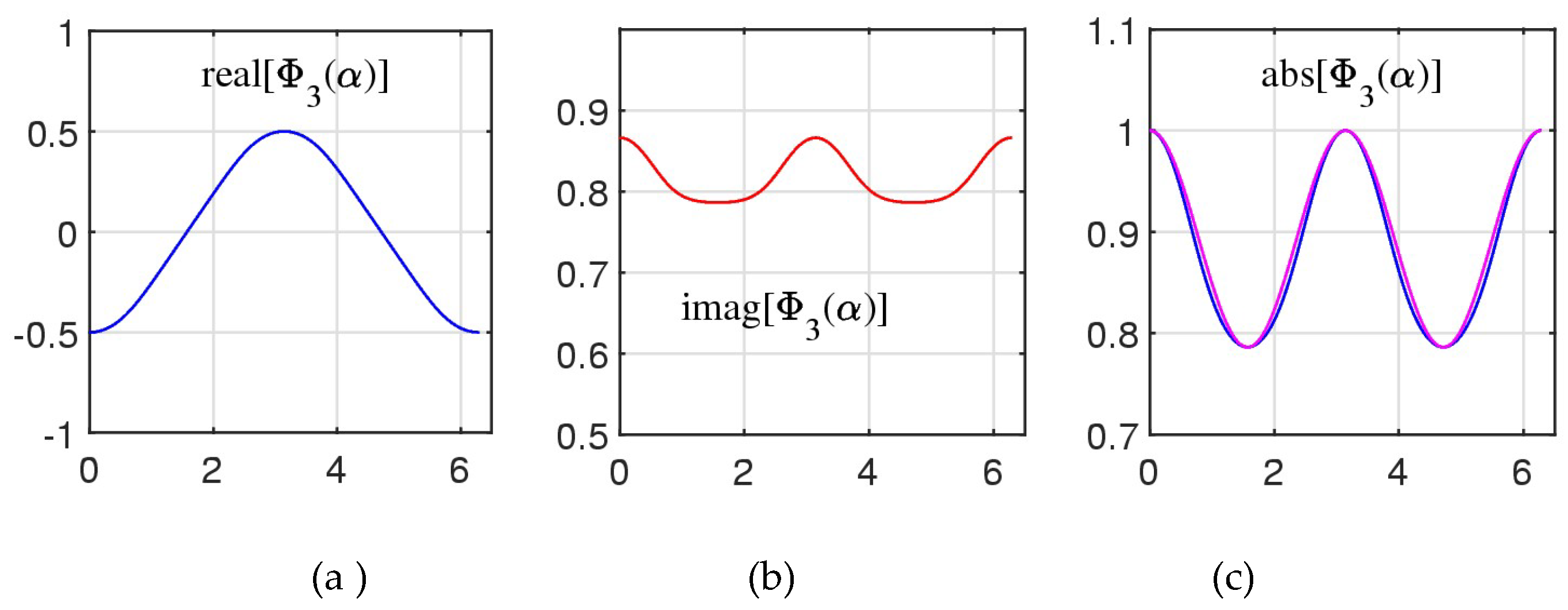
Figure 16.
Polar plots of three roots in absolute scale: (a) (b) and (c)
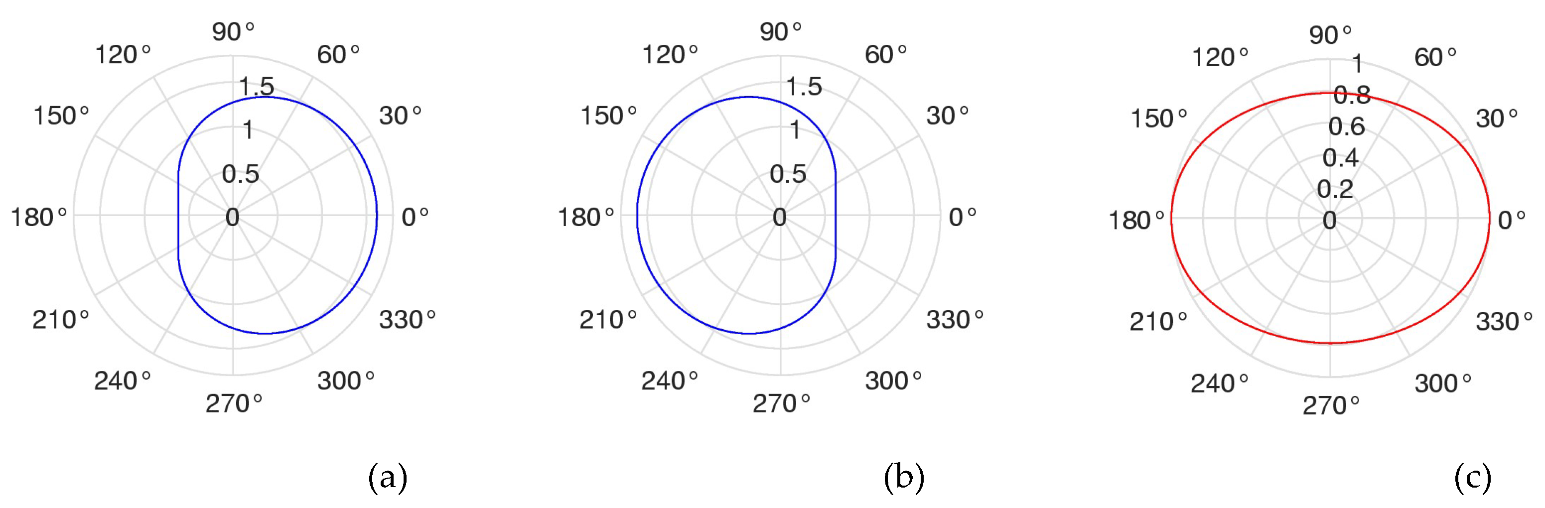
Figure 17.
2D vectors.
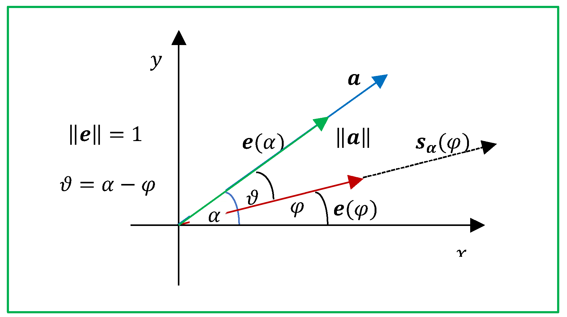
Figure 18.
The locus of 128 golden pairs with the vectors (a) and (b)
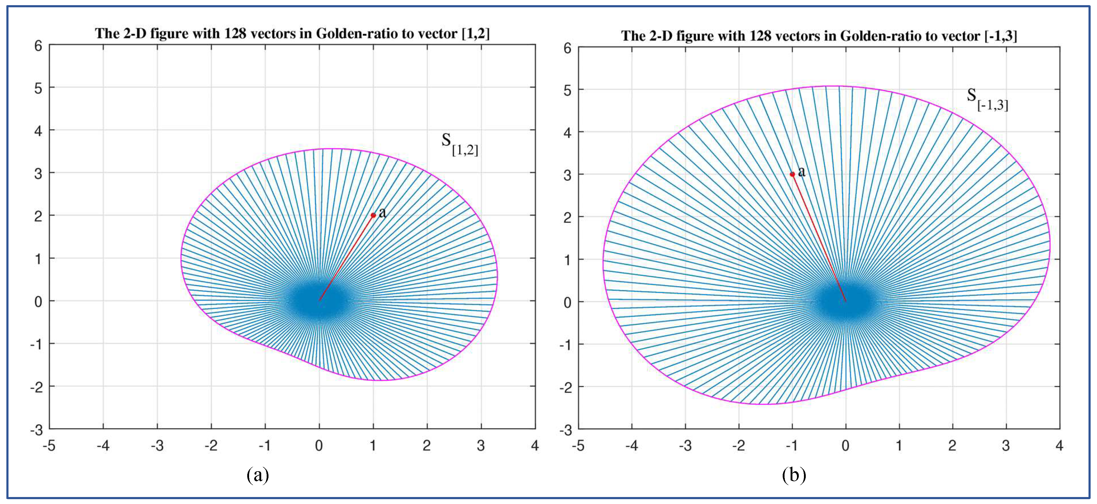
Figure 19.
The parallelogram composed of the sum of two vectors (a) before and (b) after the rotation by the angle .
Figure 19.
The parallelogram composed of the sum of two vectors (a) before and (b) after the rotation by the angle .
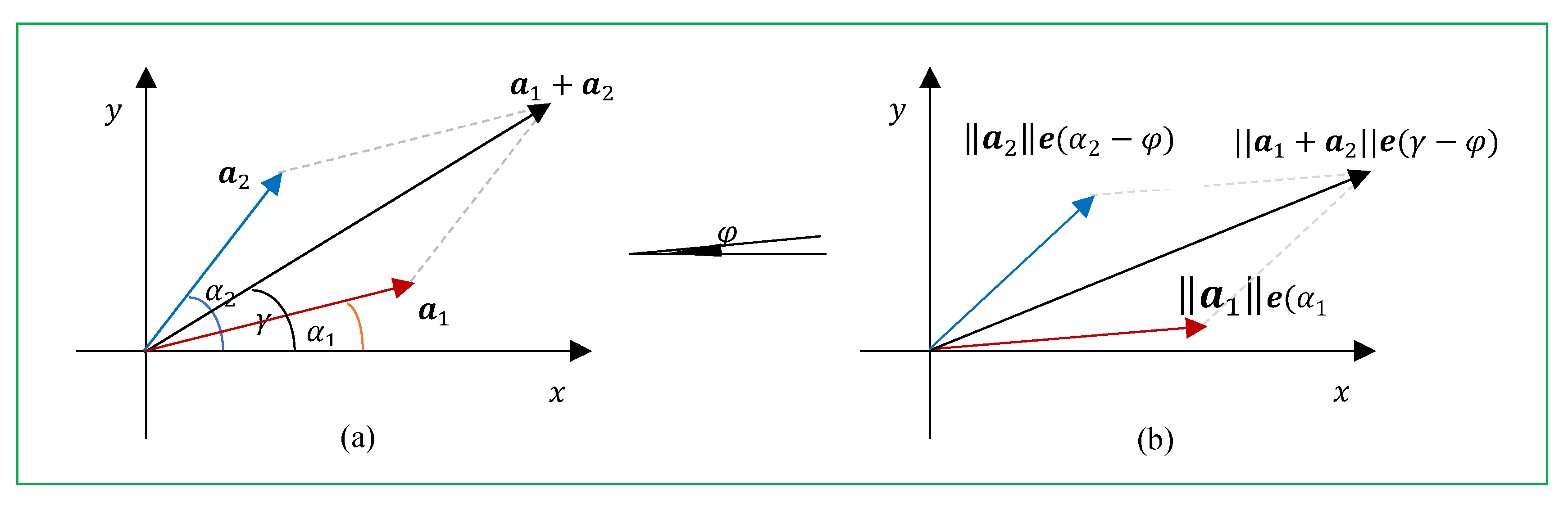
Figure 20.
Sum of similarity sets for the 2-D vectors (a) , and (b) ,
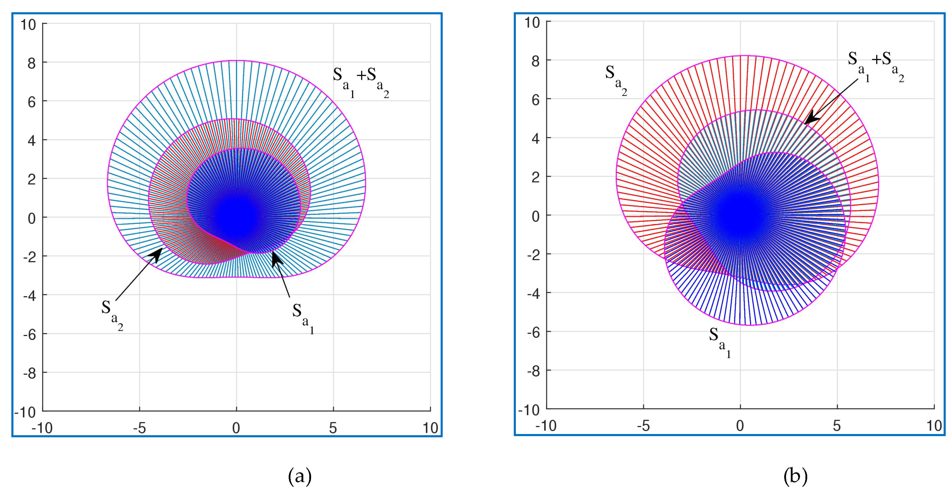
Figure 21.
Sum of similarity sets for the 2D vectors (a) , , (b) , and (c) , .
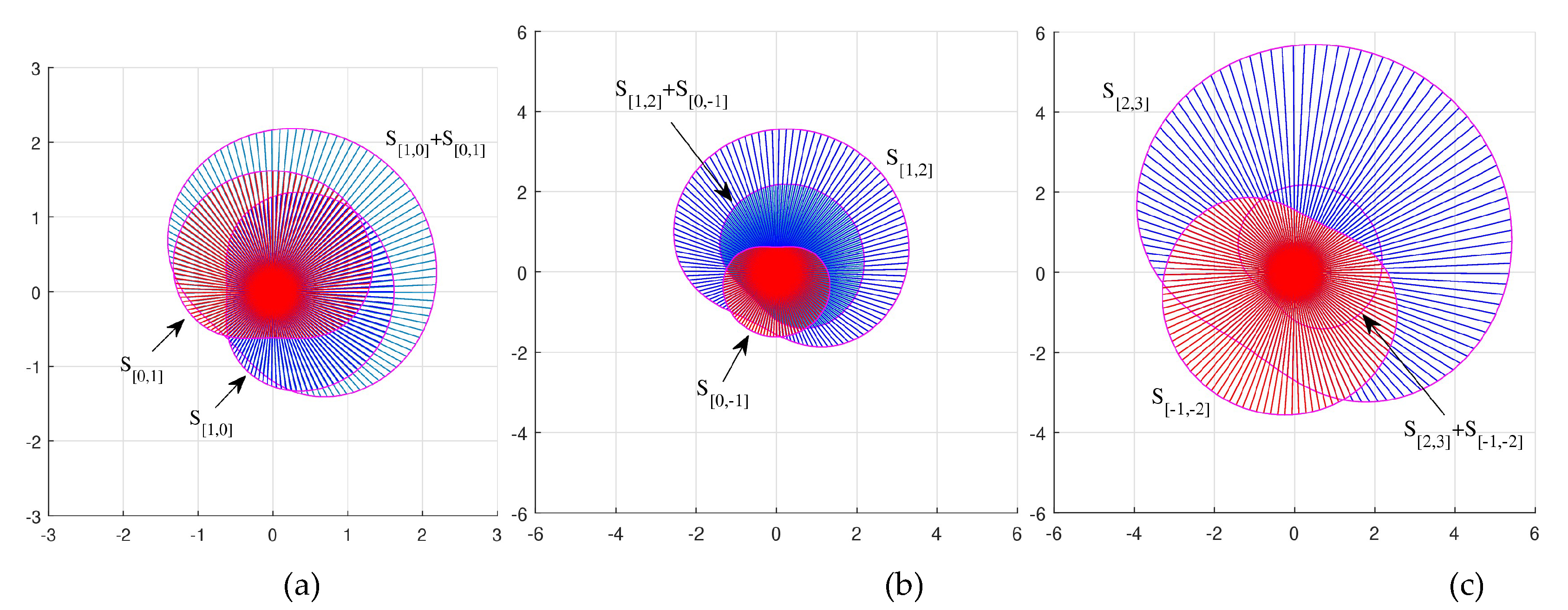
Figure 22.
The unit vector in the 3D spherical coordinate system.
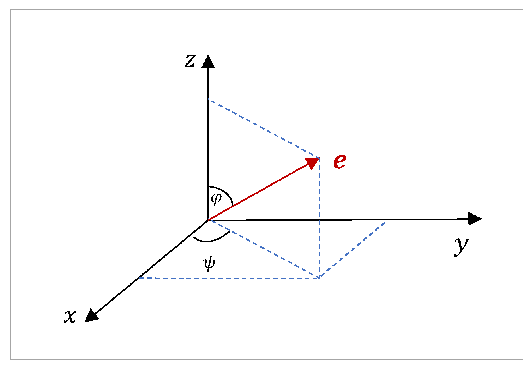
Figure 23.
The geometry of the similarity sets of golden vectors with the 3D vectors (a) [0,0,1] and (b) [1,0,0].
Figure 23.
The geometry of the similarity sets of golden vectors with the 3D vectors (a) [0,0,1] and (b) [1,0,0].
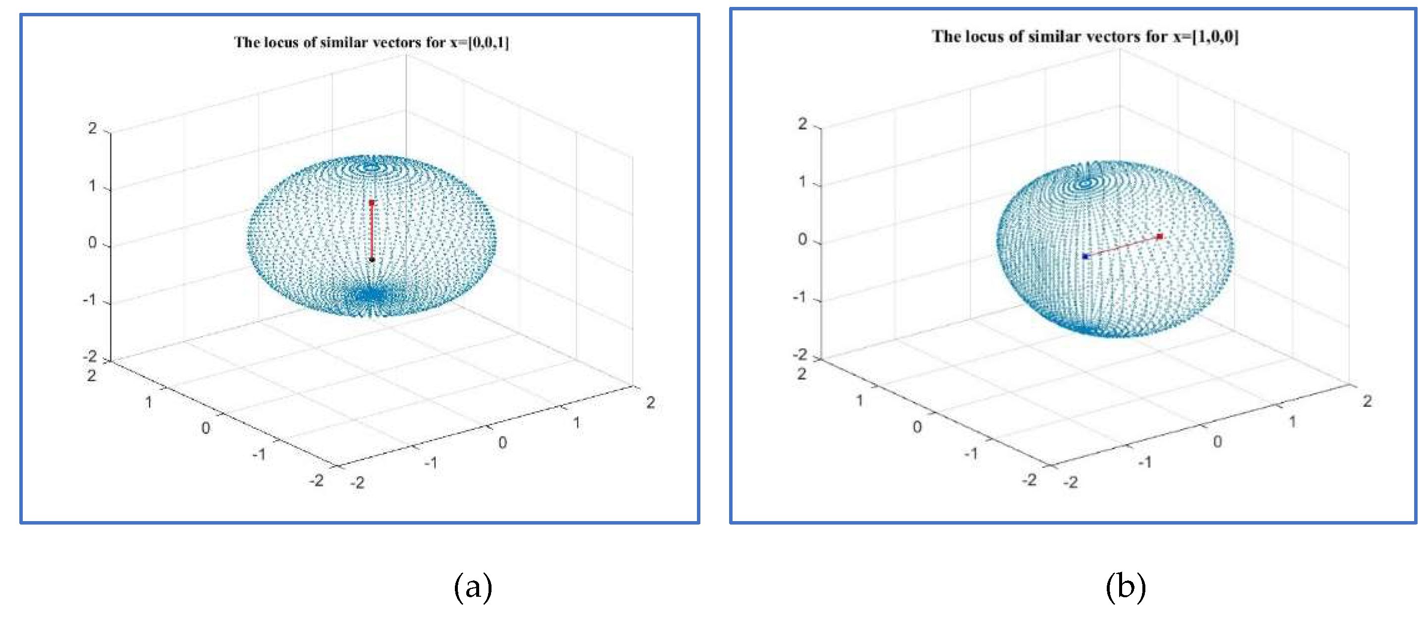
Figure 24.
The view with AZ=0 and EL=90 degrees of the geometry of similarity sets of the Golden vectors with the 3D vectors (a) [0,0,1] and (b) [1,0,0].
Figure 24.
The view with AZ=0 and EL=90 degrees of the geometry of similarity sets of the Golden vectors with the 3D vectors (a) [0,0,1] and (b) [1,0,0].
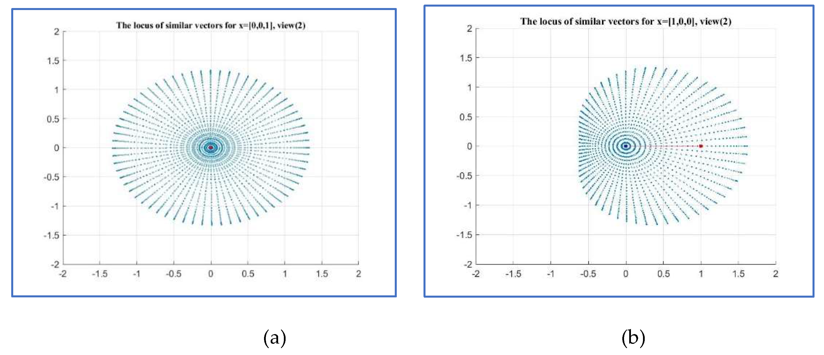
Figure 25.
The view with AZ=0 and EL=180 degrees: The geometry of the similarity sets of the Golden vectors with the 3-D vectors (a) [0,0,1] and (b) [1,0,0].
Figure 25.
The view with AZ=0 and EL=180 degrees: The geometry of the similarity sets of the Golden vectors with the 3-D vectors (a) [0,0,1] and (b) [1,0,0].
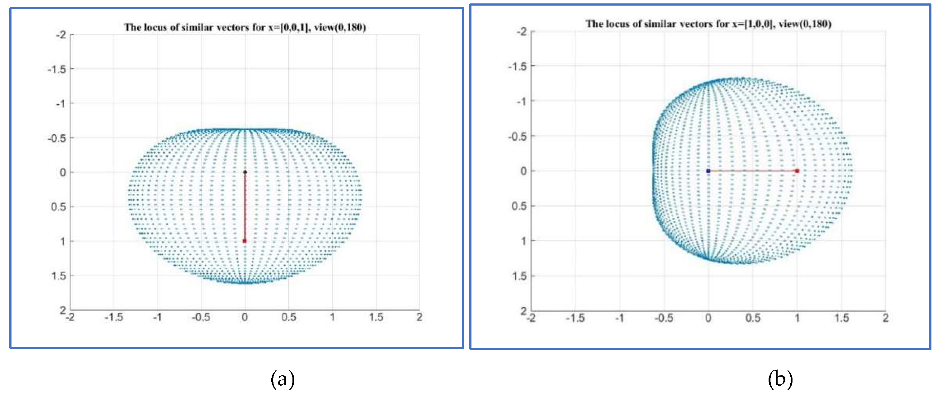
Figure 26.
The 3-D surface of the similarity sets of the Golden vectors with the 3-D vectors (a) [0,0,1] and (b) [1,0,0].
Figure 26.
The 3-D surface of the similarity sets of the Golden vectors with the 3-D vectors (a) [0,0,1] and (b) [1,0,0].
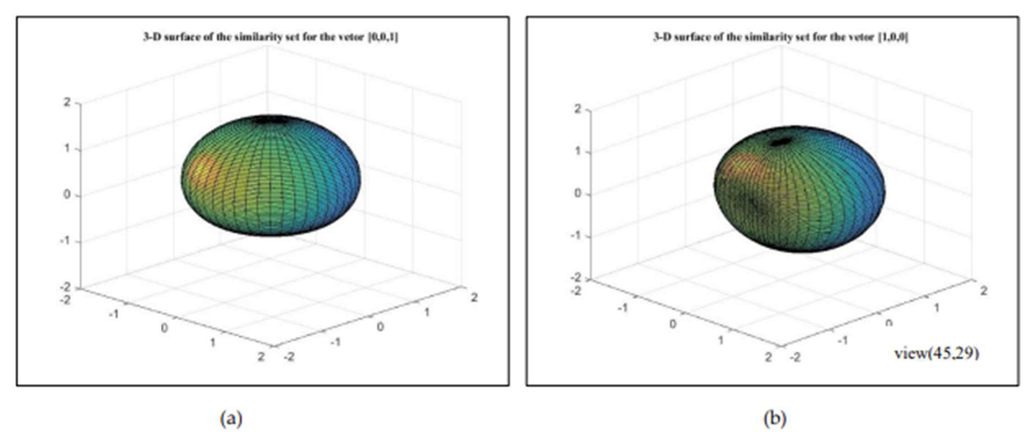
Figure 27.
(a) Triangle for the vector and (b) the triangle with the vertex at the origin.
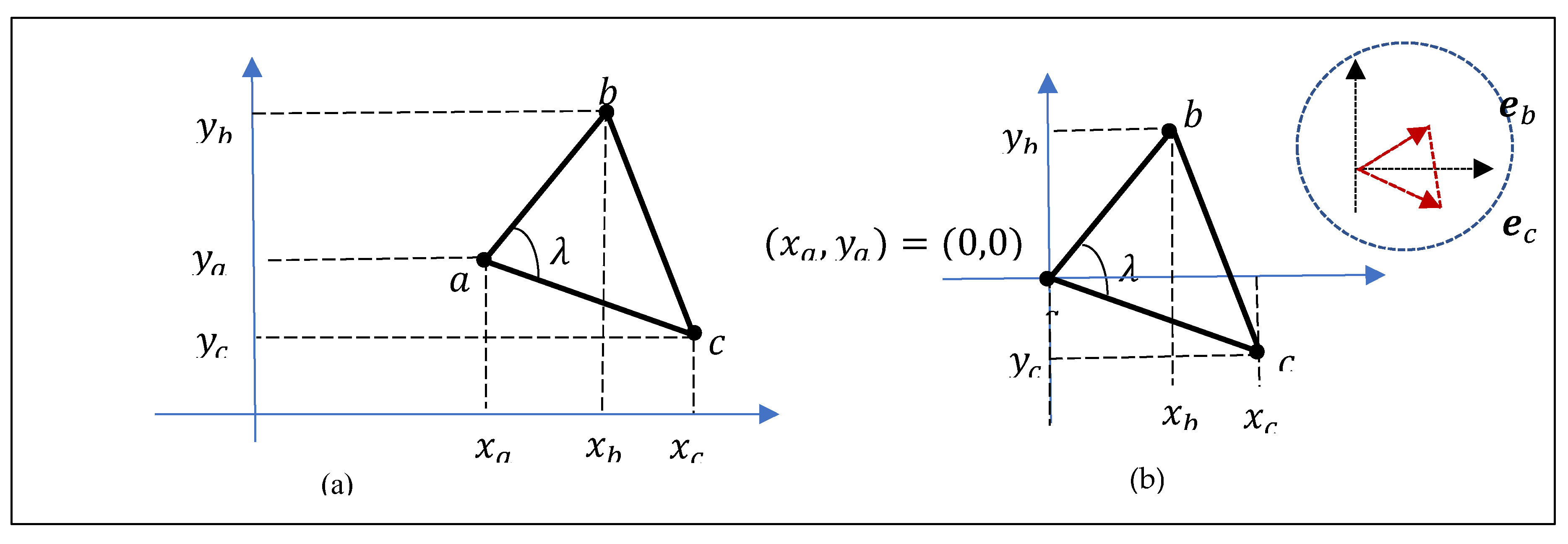
Figure 28.
Five unit triangles with the angle
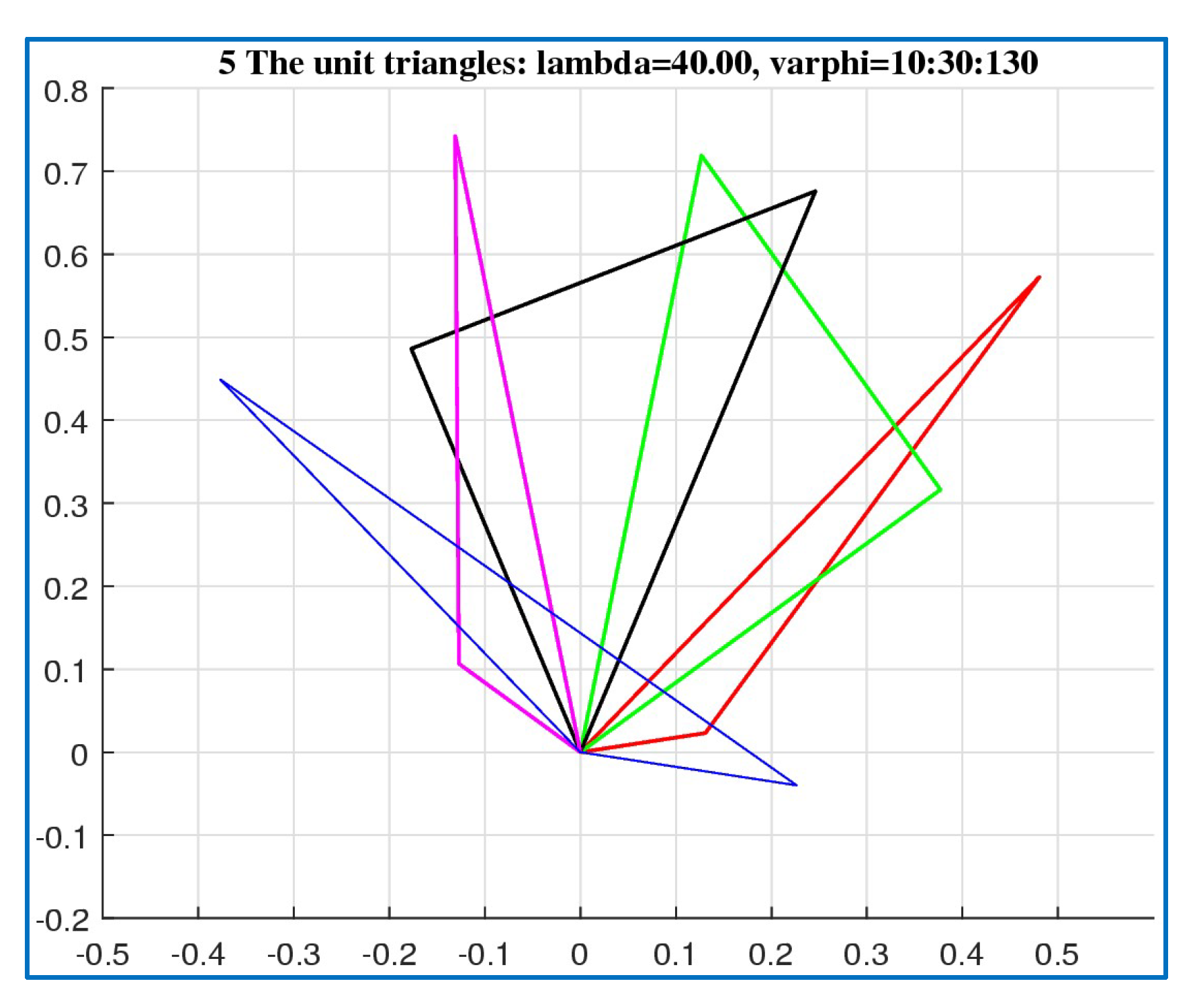
Figure 29.
The unit triangles with the angle (a) and (b)
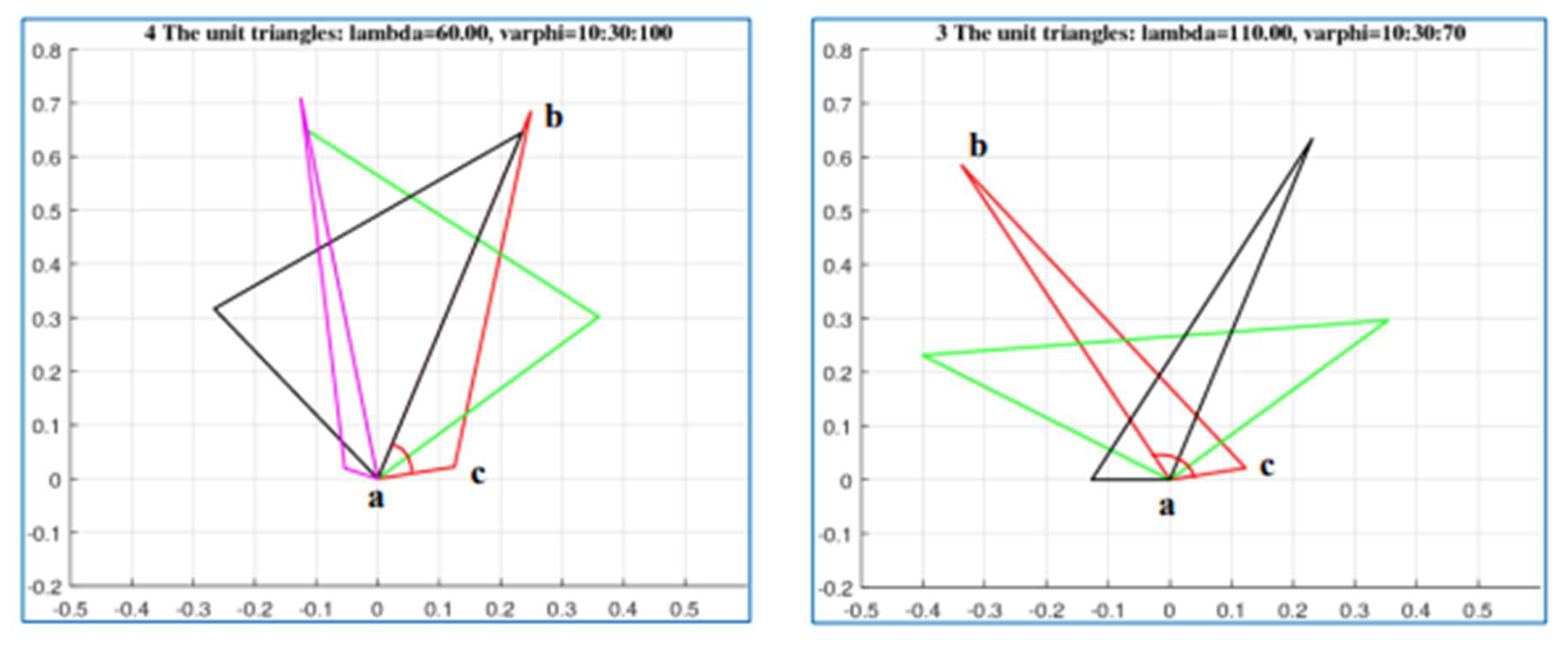
Figure 30.
(a) The original triangle with angle and similarity triangles with the angle of (b) (c) and (d)
Figure 30.
(a) The original triangle with angle and similarity triangles with the angle of (b) (c) and (d)
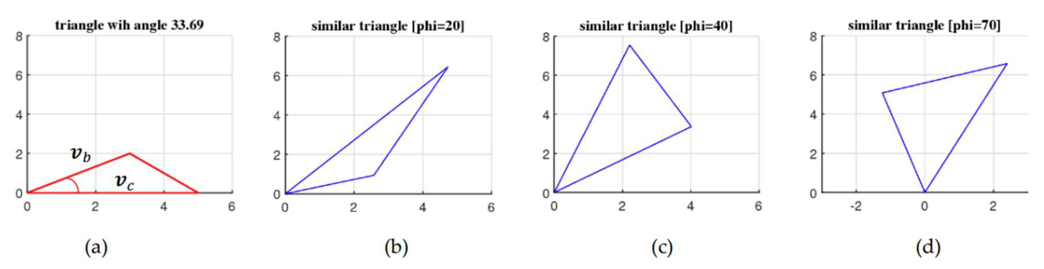
Figure 31.
The similarity triangles for (a) the triangle with angle and (b) the triangle with angle . .
Figure 31.
The similarity triangles for (a) the triangle with angle and (b) the triangle with angle . .
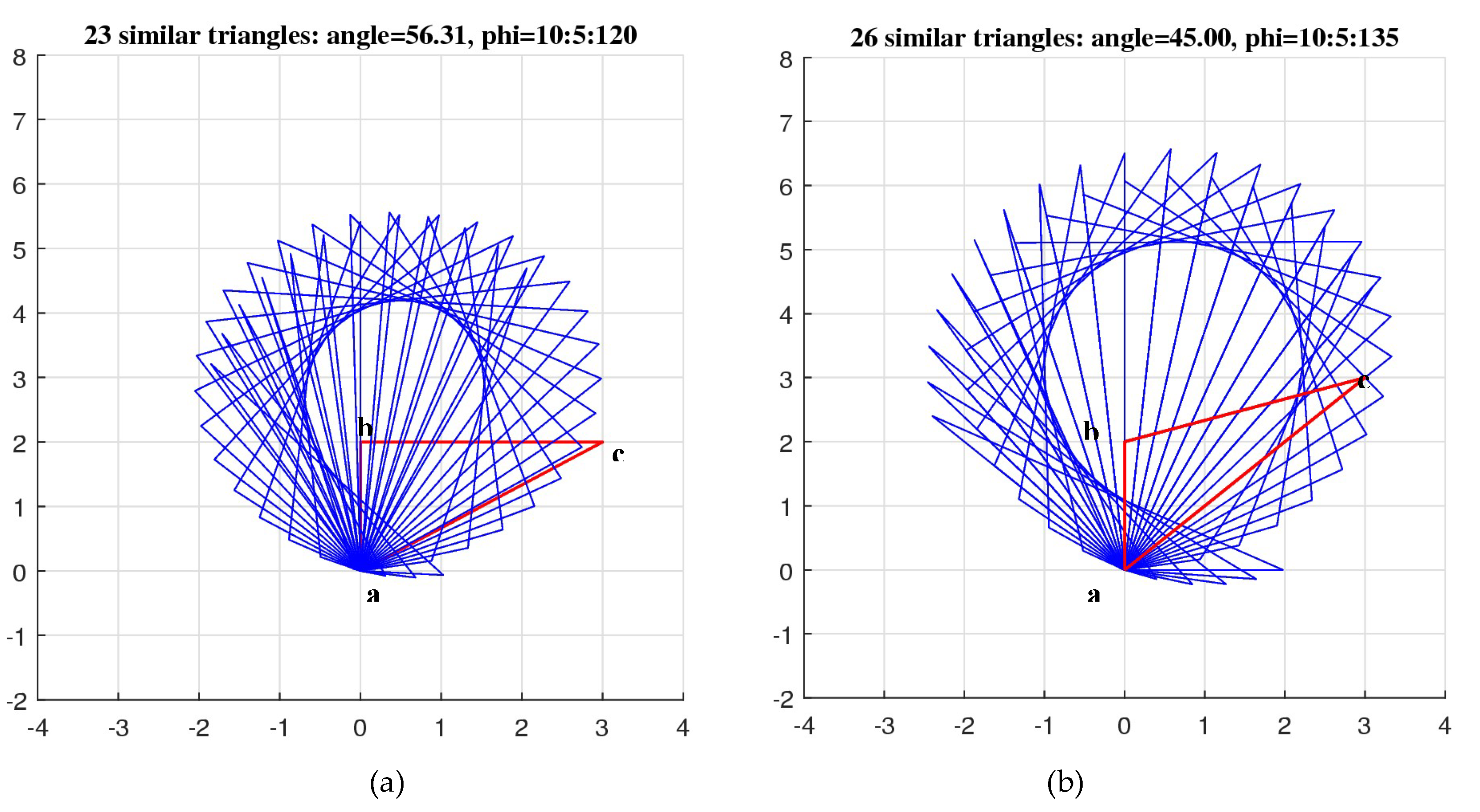
Figure 32.
The similarity triangles for the equilateral triangle, when the angle (a) and (b) .
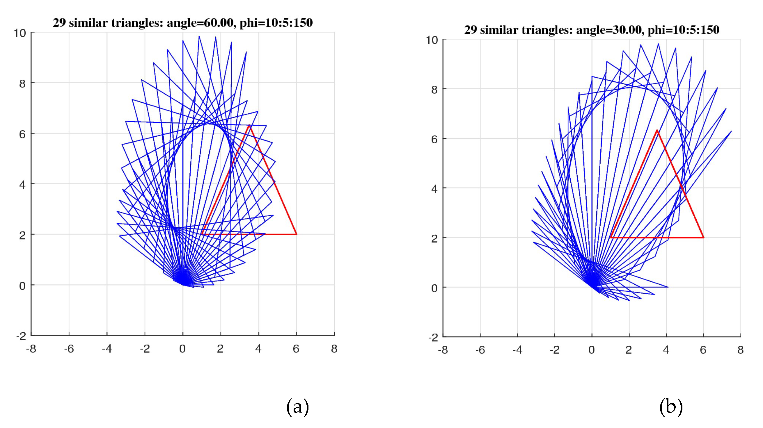
Figure 33.
(a) The original and rotated triangles, (b) the original triangle and its two pairs, and (c) the same shaded triangles.
Figure 33.
(a) The original and rotated triangles, (b) the original triangle and its two pairs, and (c) the same shaded triangles.
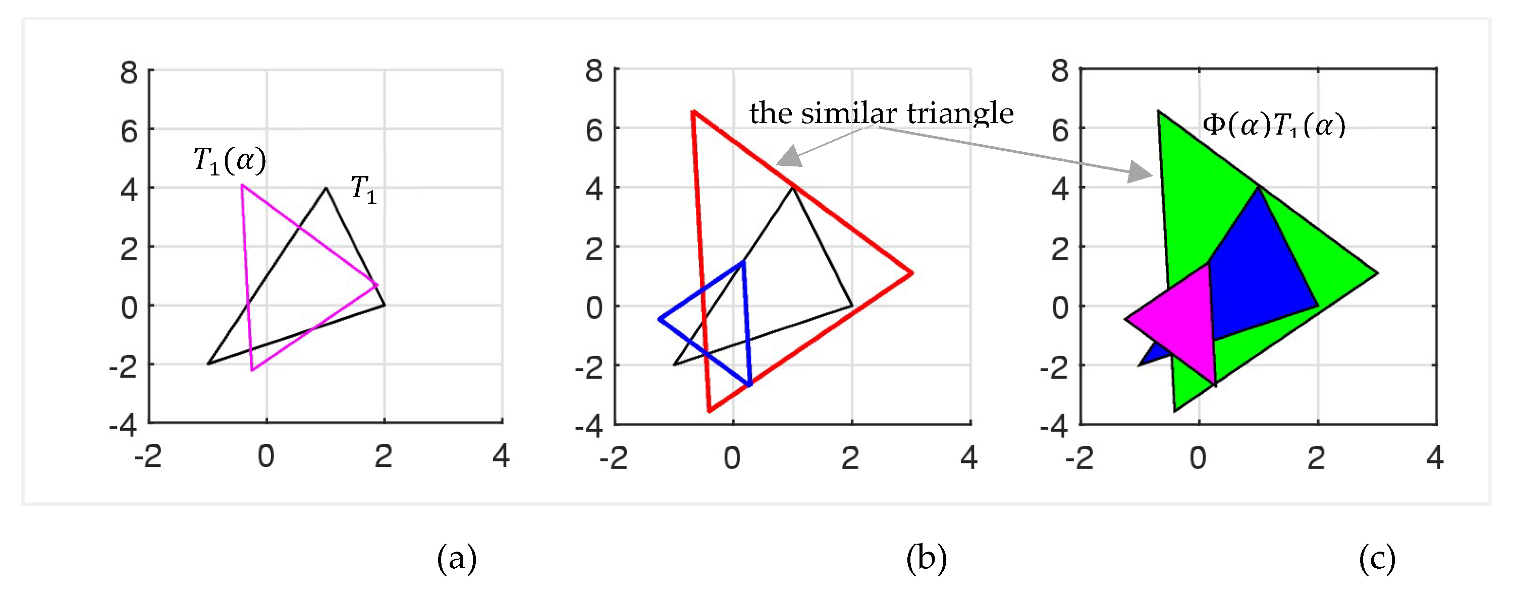
Figure 35.
The heptagon and its golden pairs for the angles 30,140, -100, and 200. (roos4_2.m)
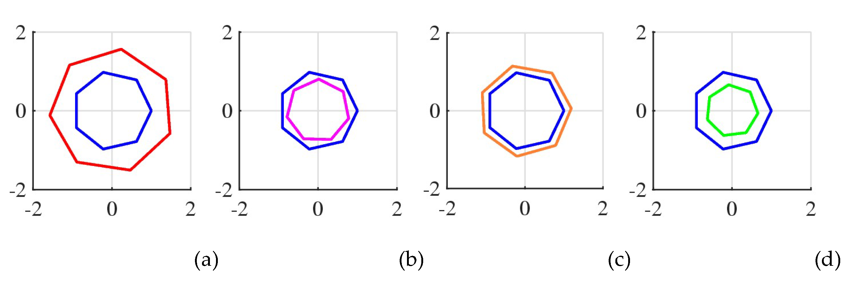
Figure 36.
The heptagram and its golden pairs for the angles 30,90,160, and 220.
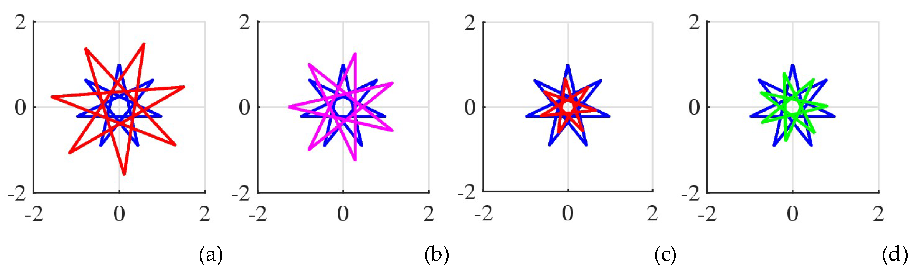
Figure 37.
(a) The enneagram and its golden pairs for the angles (b) 90, (c) 160, and (d) 220.
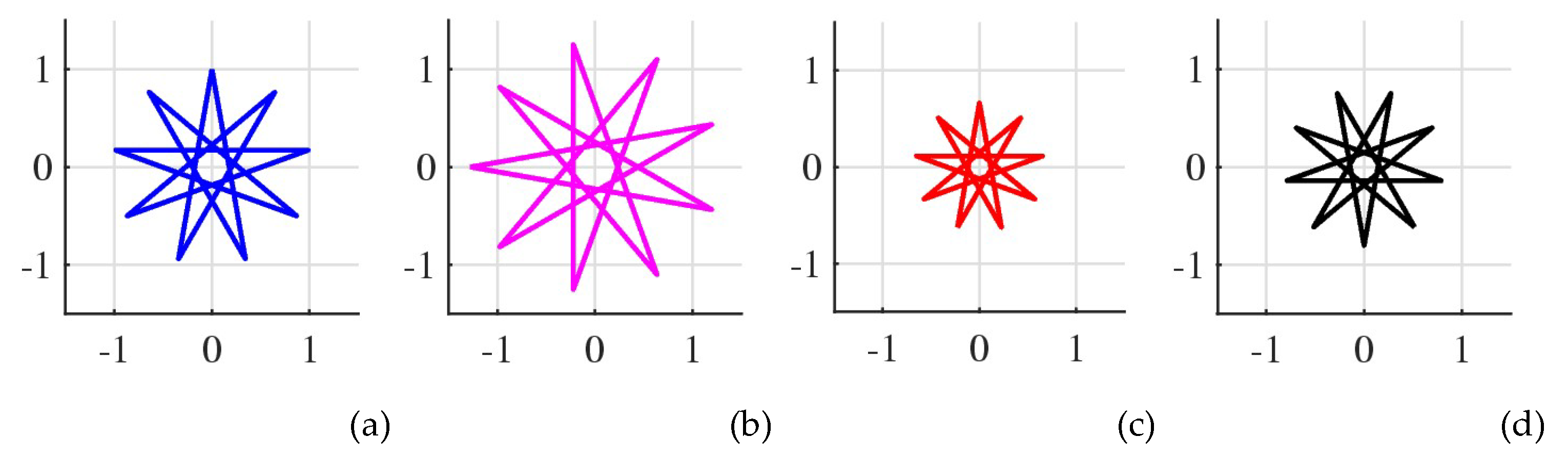
Figure 38.
The cross together with (a) 10 equal small crosses, (b) 10 golden pairs, and (c) 12 golden pairs.
Figure 38.
The cross together with (a) 10 equal small crosses, (b) 10 golden pairs, and (c) 12 golden pairs.
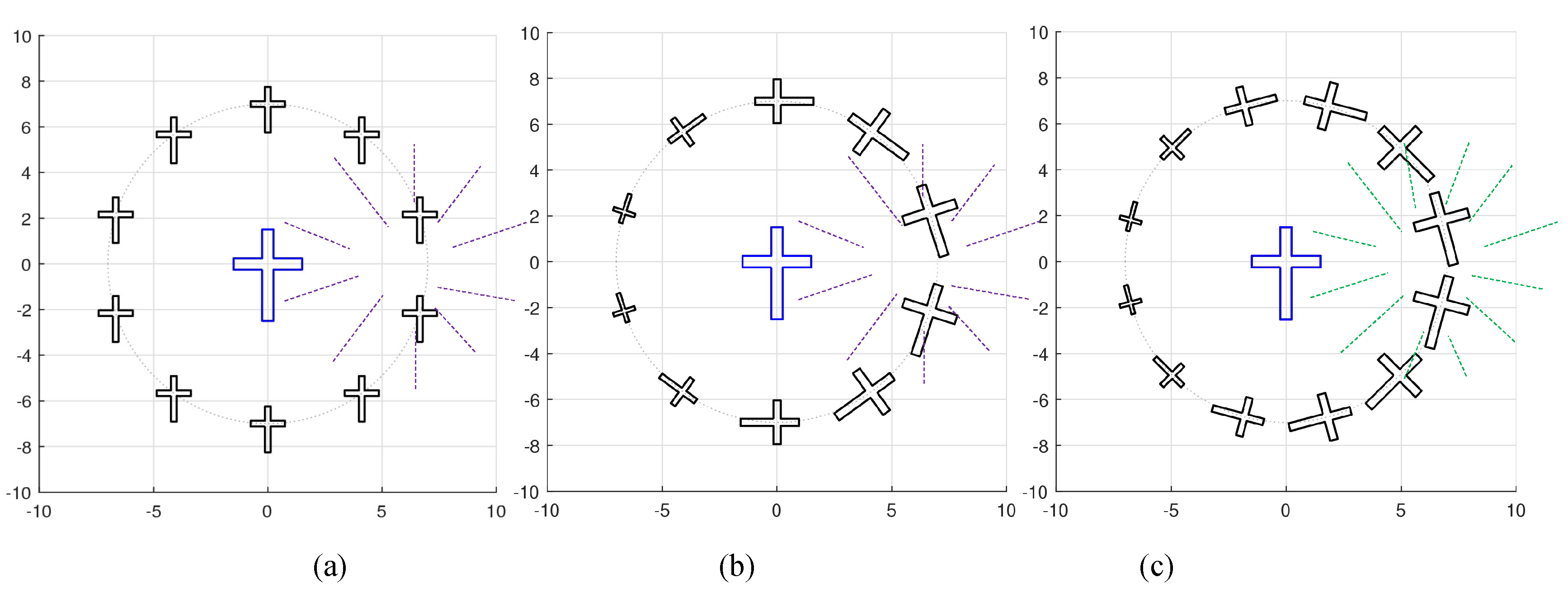
Figure 39.
The star together with (a) 12 equal small stars and (b) 12 stars of the golden pairs.
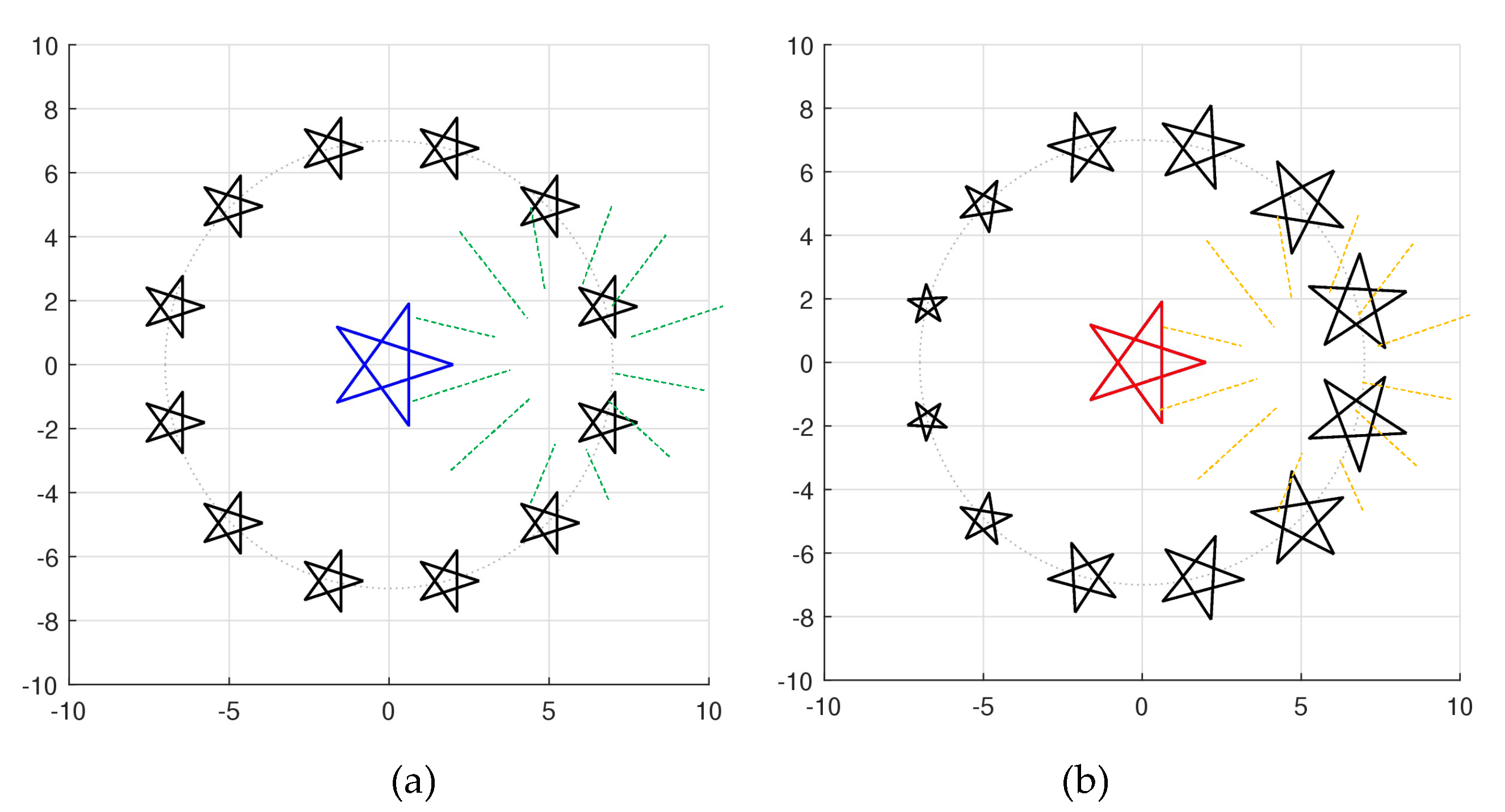
Figure 40.
The 7-pointed and 9-pointed stars together with their 12 stars of the golden pairs.
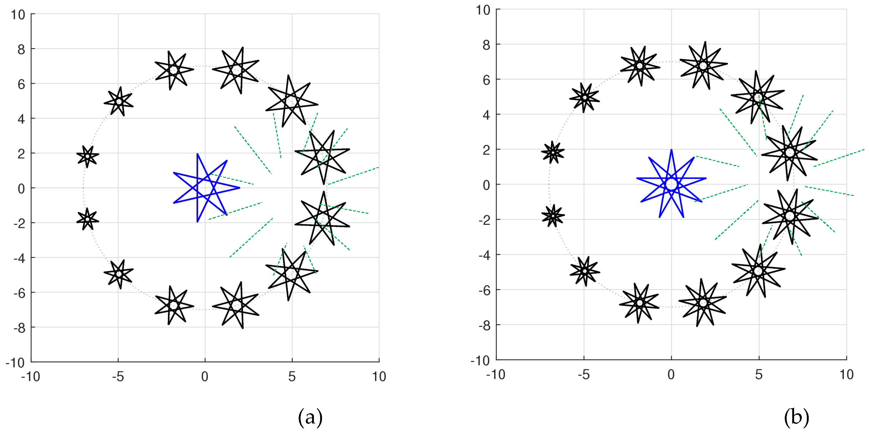
Figure 41.
The 108-points on the Archimedes spiral together with eight golden-pairs.
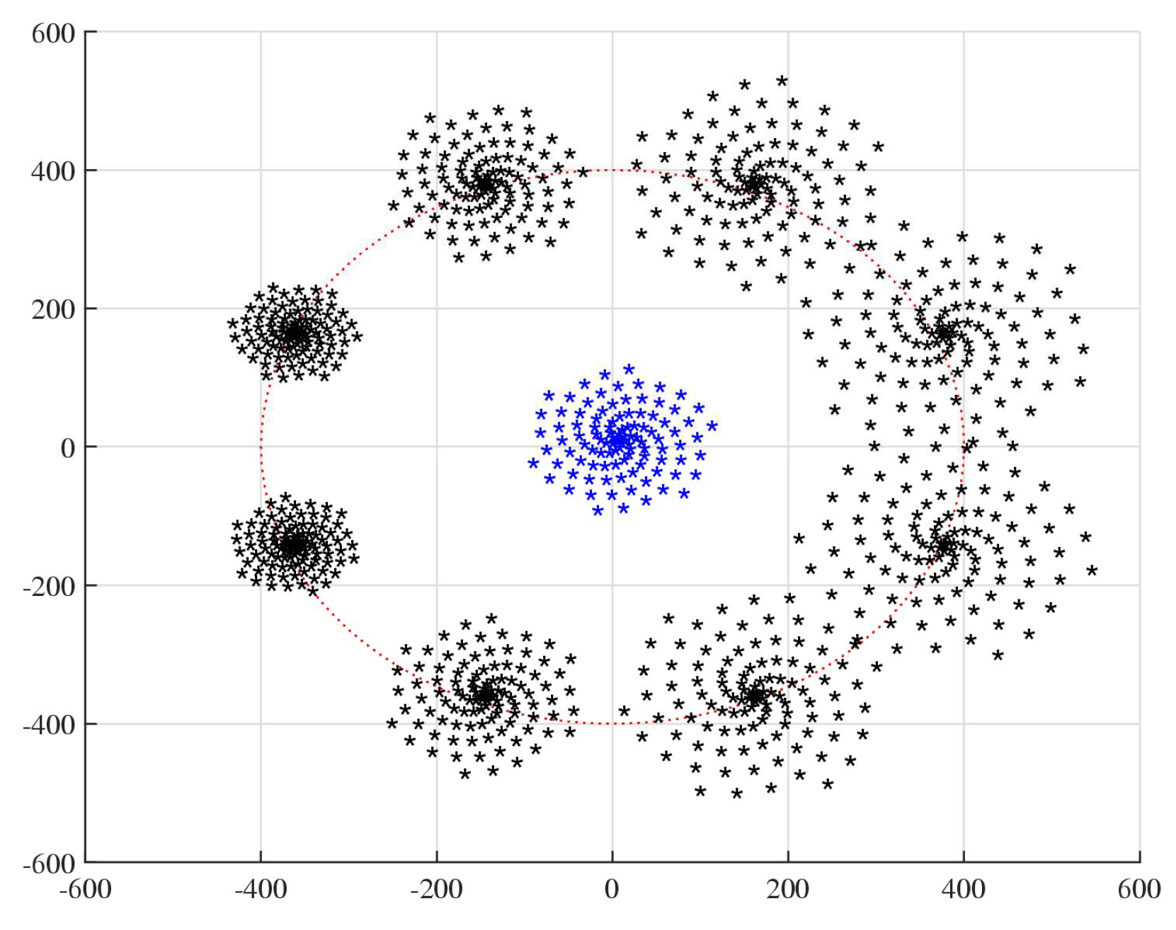
Figure 42.
The 2-D view of 108 golden (a) squares, (b) pentagons, (c) hexagons, and (d) heptagons.
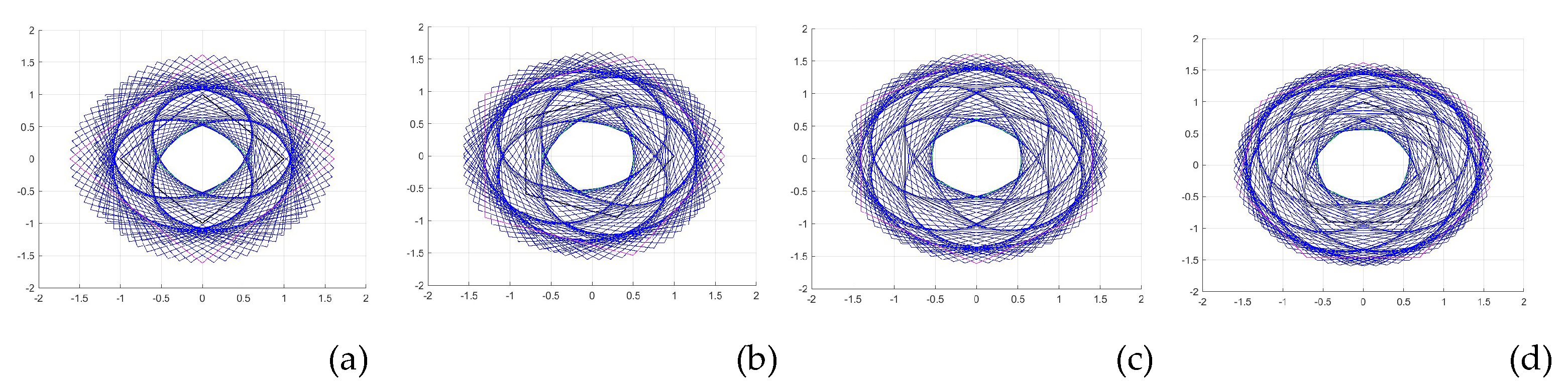
Figure 43.
3D composition of golden figures for (a) the square and (b) the dodecagon.
Disclaimer/Publisher’s Note: The statements, opinions and data contained in all publications are solely those of the individual author(s) and contributor(s) and not of MDPI and/or the editor(s). MDPI and/or the editor(s) disclaim responsibility for any injury to people or property resulting from any ideas, methods, instructions, or products referred to in the content. |
© 2025 by the authors. Licensee MDPI, Basel, Switzerland. This article is an open access article distributed under the terms and conditions of the Creative Commons Attribution (CC BY) license (http://creativecommons.org/licenses/by/4.0/).
Copyright: This open access article is published under a Creative Commons CC BY 4.0 license, which permit the free download, distribution, and reuse, provided that the author and preprint are cited in any reuse.


