Lagrangian for Non-Isolated Systems instead of Entropy for Isolated Systems

1. Introduction

In 2024 it has been 200 years since Sadi Carnot published his "Reflections on the Motive Power of Heat". Since that time Clausius, Kelvin, Maxwell, Boltzmann, Gibbs, and many other physicists and chemists have been working on entropy-based formulation and development of the Second Law of Thermodynamics for isolated systems. There are many ways to formulate the Second Law of Thermodynamics. For example, one of the axiomatic statements is: “There exists for every thermodynamic system in equilibrium an extensive scalar property called the entropy $S$, such that in an infinitesimal reversible change of state of the system, $dS=dQ/T$, where $T$is the absolute temperature and $dQ$is the amount of heat received by the system. The entropy of a thermally insulated system cannot decrease and is constant only if all processes are reversible” [1]. The purpose of this paper is to consider a more realistic case when non-isothermal systems are influenced by external fields.

Here we should remind that equilibrium Gibbs thermodynamics has three major laws, and it answers the question “How much?”, but not “How fast?”. Newtonian mechanics also is based on three laws. It answers the question “How fast?”. Indeed, the Second Law is $a=\mathrm{F}/m$, where acceleration $a$is proportional to the acting force$F$.

2. Methods

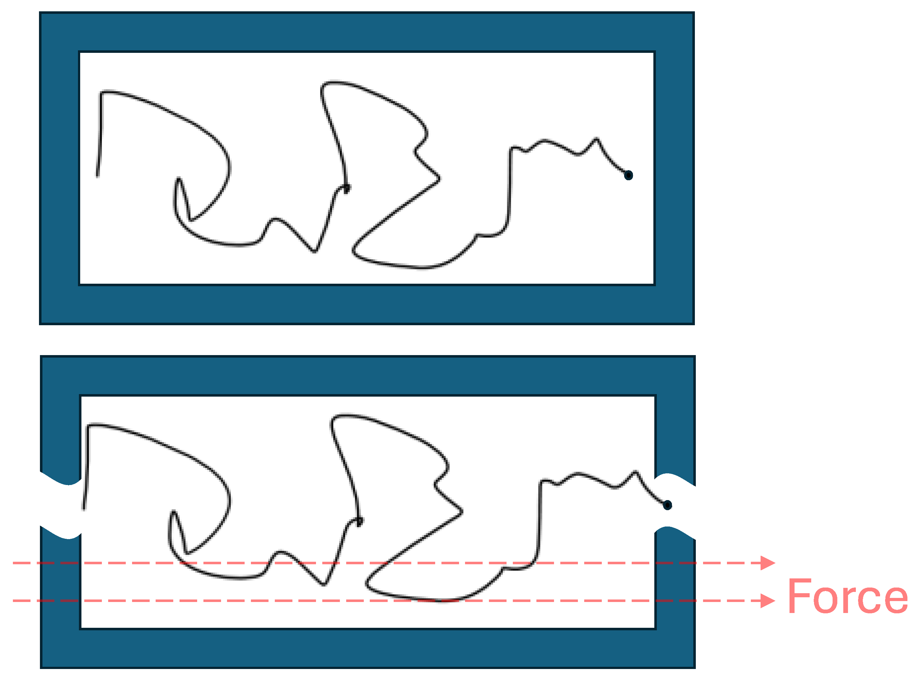
Figure 1 shows an isolated system (a); and influenced by an external force non-isolated system (b). If there are several forces, we should use ${\displaystyle \sum F_j}$. Of course, the isolated system is an idealization valid for a vacuum or a planetary system. In real systems, we should add a friction force, which is proportional to velocity, but has an opposite direction.

Very soon it becomes equal to the total of all applied forces. As a result, they balance each other, and transport reaches a steady state when the acceleration vanishes. After substitution it is the velocity and not acceleration, which becomes proportional to the total of all acting forces. In hydrodynamics, this is known as a Stokes’ equation. Instead of coefficient $1/m$ proportionality coefficient is $1/\zeta$, where $\zeta$ is proportional to the solution friction and depends on the particle shape [2]. To describe Brownian motion and diffusion of molecules Einstein suggested using molecular mobility$U$, which is $U=1/\zeta$ and is velocity per unit of acting molar force with units (cm/sec)/(newton/mol) [3]. For transport of each component, we usually need the flux J_i per unit of perpendicular area, which is proportional to the product of velocity $U_i{\displaystyle \sum _j{F}_{ji}}$ by concentration, i.e. $J_i=U_i{c}_i{\displaystyle \sum _j{F}_{ji}}$. If we deal with an ionic flux, the major driving force is the negative gradient of electric potential, multiplied by molar charge, $F_{ei}=-q_i{\displaystyle \frac{d{\psi }_e}{dx}}$, leading to Faraday’s law $J_i=U_i{c}_i{z}_{i}F{\displaystyle \frac{d\psi }{dx}}$. Here F is the Faraday constant and $z_i$ is an elementary ion charge. The product of J_i and a molar charge gives electric current, i.e. Ohm’s law, and electric conductivity is $U_i{c}_i{q}_i^2$. The same approach may be used for other fluxes and driving forces. To calculate any transport coefficient, we need only mobility and conjugated molar properties, such as molar charge, molar volume, etc. Based on the same mobility method is valid for major colloid and surface transport processes [4].

This approach [5,6], which we call physicochemical mechanics, allows systematic derivation of all major transport laws and their equilibrium relations. We described the rates of transport processes in non-isolated systems, influenced by external fields and how they reach equilibrium. For seven major driving factors, we suggested a Table with more than 7x7 transport laws and their equilibrium relations [7]. The typical value of these driving factors decreases from the left to the right column, and from the upper to the lower horizontal line. The Table may grow further if we add new driving factors, including mechanical deformations of solids or even optical trapping of single molecules [6].

Recalling that based on his Periodic Table of elements D. Mendeleev predicted properties of four yet unknown elements [8], we predicted one new phenomenon, which we called magneto tension [7]. In this case deformation of the liquid surface by a magnetic field is observed. Later, it was confirmed in experiments, and now it is called the Moses effect [9], reminding the description in the Old Testament of crossing of the Red Sea by Jews led by Moses.

3. Results

3.1. General Equation

Previously to describe transport of a chemical component i in isothermal and not isolated systems we suggested using a new general physicochemical potential, ${\mu }_{gi}$, where ${\mu }_{gi}={\mu }_i+{\displaystyle \sum _{j-1}{\chi }_{j-1}}{\psi }_{j-1}$. Here, ${\mu }_i={\mu }_{0i}+RT\ln c_i$ is the traditional chemical potential of this component. ${\psi }_{j-1}(x)$is the local field potential, and ${\chi }_{j-1}$is the conjugated molar property. For example, for electric field ${\psi }_e$ ${\chi }_e$ is the molar charge and ${\mu }_{ei}={\mu }_i+{\chi }_{ei}{\psi }_e$ is known as an electrochemical potential. The negative gradient $-d{\mu }_{gi}/dx$gives the total local force leading to transport of i. This potential-based conservative force does not depend on velocity [5]. Without external potential fields or for isolated systems it is reduced to traditional chemical potential, which is molar isobaric-isothermal Gibbs energy.

Chemical energy in transport processes dissipates into heat. Now, if local temperature also changes in the system, instead of used for isothermal processes gradient of chemical potential $-d{\mu }_i/dx$, because of energy dissipation into heat we suggest using

$${\displaystyle \frac{d{q}_i}{dx}}={\displaystyle \frac{d(s_{i}T)}{dx}}={\displaystyle \frac{Td{s}_i}{dx}}+{\displaystyle \frac{s_{i}dT}{dx}}$$

(1)

Here $s_i$is the local molar entropy of i-th component and q_i is its local molar heat (not charge!). Both terms ${\displaystyle \frac{Td{s}_i}{dx}}$ and ${\displaystyle \frac{s_{i}dT}{dx}}$ have units of molar force and may be called the entropic and thermal forces. They have positive signs, reflecting, for example, that at constant temperature the process is directed to the increase of entropy (the Second Law). Another typical situation is when the elementary process, such as movement of a piston, is isothermal, and ${\displaystyle \frac{s_{i}dT}{dx}}=0$.

Here it makes sense to recall the well-known phrase by J.W. Gibbs: “If we wish to find in rational mechanics an a priory foundation for the principles of thermodynamics, we must seek mechanical definition of temperature and entropy” [10]. Each conservative potential force $F_{ji}$ is proportional to the space gradient of its potential with a minus sign and it should be counteracting entropic force, i.e., an increase of entropy due to dissipation. In the steady state the total of the external forces minus thermal and entropic forces is balanced by friction forces and the directed mass transport reaches constant velocity. In equilibrium the total acting force minus thermal and entropic forces is zero, the total flux vanishes, and no directed friction counterforces are formed. According to the Second Law, the entropy of a closed isolated system in a spontaneous process increases and at equilibrium it reaches maximum. Now it is clear that this maximum is determined by the balance of entropic and other internal forces. At equilibrium only without external forces local temperature and entropy are constant and do not depend on x, giving suggested by Clausius $d{s}_i=d{q}_i/T$. For the whole Universe, this imaginary state is known as the heat death of the Universe.

In the presence of external forces, we have a general equation

$$J_i=U_i{c}_i({\displaystyle \frac{s_{i}dT}{dx}}+{\displaystyle \frac{Td{s}_i}{dx}}+{\displaystyle \sum _j{F}_{ji}})$$

(2)

3.2. Clausius Inequality, Fokker-Planck-Smoluchowski, Nernst and Van’t Hoff Laws

To understand this equation better, as usual, we will start with an ideal gas. It is known that at equilibrium molar entropy of an ideal gas per unit volume is $\mathrm{s}\hspace{0.17em}{=\mathrm{s}}_o-R\ln c+C_{\mathrm{v}}\ln T$[11], where $C_{\mathrm{v}}$is heat capacity. This expression should also be valid for local entropy in transport processes. Without ${\displaystyle \sum _j{F}_{ji}}$

$${\displaystyle \frac{d{q}_i}{dx}}={\displaystyle \frac{d(s_{i}T)}{dx}}=({\mathrm{s}}_{oi}-R\ln c_i+C_{\mathrm{vi}}\ln T){\displaystyle \frac{dT}{dx}}\hspace{0.17em}+T({\displaystyle \frac{d{s}_{0i}}{dx}}-{\displaystyle \frac{R}{c_i}}{\displaystyle \frac{d{c}_i}{dx}}+{\displaystyle \frac{C_{Vi}}{T}}{\displaystyle \frac{dT}{dx}})$$

After simplification, it is reduced to

$$d{s}_i={\displaystyle \frac{d{q}_i}{T}}-({\mathrm{s}}_{oi}-R\ln c_i+C_{\mathrm{vi}}\ln T){\displaystyle \frac{dT}{T}}$$

This leads to the well-known Clausius inequality $d{s}_i\ge {\displaystyle \frac{d{q}_i}{T}}$. In addition, when internal heat is used by gas to move a piston without equilibrium, the gas temperature decreases.

The flux becomes

$$J_i=U_i{c}_i{\displaystyle \frac{d{q}_i}{dx}}=U_i{c}_i[T({\displaystyle \frac{d{s}_{0i}}{dx}}-{\displaystyle \frac{R}{c_i}}{\displaystyle \frac{d{c}_i}{dx}})+({\mathrm{s}}_{oi}-R\ln c_i+C_{\mathrm{vi}}\ln T+C_{\mathrm{v}i}){\displaystyle \frac{dT}{dx}}]$$

(3)

Some simplifications are interesting:

• Both ${\mu }_i$ and $s_i$have the term Rlnc but with opposite signs. In the homogeneous and isothermal system ${\displaystyle \frac{d{s}_{0i}}{dx}}=0$ and $\hspace{0.17em}{\displaystyle \frac{dT}{dx}}=0$, leading to Fick’s law of diffusion $J_i=-RT{U}_i{\displaystyle \frac{d{c}_i}{dx}}=-D_i{\displaystyle \frac{d{c}_i}{dx}}\hspace{0.17em}\hspace{0.17em}$and Fokker-Einstein relation $D_i=RT{U}_i$. Mass conservation law ${\displaystyle \frac{dc}{dt}}=-{\displaystyle \frac{dJ}{dx}}$ in the presence of fields leads to the Fokker-Planck-Smoluchowski equation${\displaystyle \frac{\partial c}{dt}}=U{\displaystyle \frac{\partial }{\partial x}}[RT{\displaystyle \frac{\partial }{\partial x}}-{\displaystyle \sum _j{F}_j}]c$ [12]. Without external fields it is reduced to the Second Fick’s law of diffusion:

$${\displaystyle \frac{\partial c}{\partial t}}=RTU{\displaystyle \frac{{\partial }^{2}c}{\partial x^2}}$$

• When diffusion-driven ion flux is balanced by an electric field-driven flux in the opposite direction, in equilibrium $J_{Fick}=-J_{Faraday}$ and $-RT{U}_i{\displaystyle \frac{d{c}_i}{dx}}=U_i{c}_i{z}_{i}F{\displaystyle \frac{d\psi }{dx}}$. After integration it gives the Nernst law: $\Delta \psi ={\displaystyle \frac{RT}{z_{i}F}}\ln {\displaystyle \frac{c_1}{c_2}}$. For pressure we have $\Delta P={\displaystyle \frac{RT}{ \mathrm{v} ¯}}\ln {\displaystyle \frac{c_1}{c_2}}\simeq {\displaystyle \frac{RT}{ \mathrm{v} ¯}}\Delta c$. Thus, for small $\Delta c$we have Van’t Hoff law for osmotic pressure [11]. Instead of logarithmic dependences for concentrations, for the balance of electric field- and pressure-driven fluxes we have ${\displaystyle \frac{d\psi }{dP}}=-{\displaystyle \frac{ \mathrm{v} ¯}{z_{i}F}}=const$. Similar types of equilibrium relations should be valid for other potential-based forces at constant temperature.

3.3. Thermodiffusion. Soret and Dufour Effects

If the initial concentration is constant, and we have only a temperature gradient along the space coordinate x as a driving factor, the process is called thermodiffusion or the Soret effect. The flux should be

$$J_i=U_i{c}_i(C_{\mathrm{v}i}+s_{oi}-R\ln c_i+C_{\mathrm{v}i}\ln T){\displaystyle \frac{dT}{dx}}=-D_{Ti}{c}_i{\displaystyle \frac{dT}{dx}}$$

(4)

with thermodiffusion coefficient $D_{Ti}$. The Soret coefficient is the ratio S_T=D_Ti/D. The signs in front of terms with lnc and lnT are different, and we have two possible situations:

$a.\hspace{0.17em}\hspace{0.17em}\mathrm{If} \left|\ln c_i\right|\hspace{0.17em}<{\displaystyle \frac{s_{oi}+C_{\mathrm{v}i}(1+\ln T)}{R}}\hspace{0.17em}\hspace{0.17em}$, the temperature-driven flux is positive and directed to the hot side.

$\hspace{0.17em}b.\hspace{0.17em}\hspace{0.17em}\mathrm{If}\ln c_i>{\displaystyle \frac{s_{oi}+C_{\mathrm{v}i}(1+\ln T)}{R}}$, the flux is negative and directed to the cold side.

For ion transport through polymer membranes, the effect depends on both polymer and ion. For example, with 1 mM KCl solution at temperatures below 311K the direction of flux through the phenolsulfonic acid membrane was from the hot to the cold side, and at higher temperatures the flux was from the cold to the hot side [13]. It is possible to estimate at what concentration the flux should change its direction. Assuming that $J_i=$0, $s_{oi}=0$, and T=300K, and using that for one degree of freedom $C_{\mathrm{v}i}=R/2$, we get c=28.5 mol/m³ or 28.5 mM. Thus, our physicochemical mechanics approach leads to simple explanation why the flux changes its direction as the result of minor changes of temperature and concentration.

With time concentration gradient will be formed. In equilibrium of two driving factors, assuming for simplicity that ${\displaystyle \frac{d{s}_{0i}}{dx}}=0$,$C_{\mathrm{v}i}\ln T=0$, and $R\ln c_i=0$.

$$J_i=U_i{c}_i[T(-{\displaystyle \frac{R}{c_i}}{\displaystyle \frac{d{c}_i}{dx}})+(s_{0i}+C_{\mathrm{v}i}+C_{\mathrm{v}i}\ln T){\displaystyle \frac{dT}{dx}}]=0$$

$$(s_{0i}+C_{\mathrm{v}i})d\ln T=Rd\ln c_i$$

Further, using that established temperature difference is also small, after simplifications

$${\displaystyle \frac{\Delta T}{T_1}}\simeq {\displaystyle \frac{R}{s_{0i}+C_{\mathrm{v}i}}}{\displaystyle \frac{\Delta c_i}{c_{i1}}}$$

Usually, ${\displaystyle \frac{s_{0i}+C_{\mathrm{v}i}}{R}}>1$, and if $c_{i2}>c_{i1}$, we have $T_2>T_1$. Thus, the concentration gradient leads to small temperature gradient (known as the Dufour effect), and in considered conditions the higher temperature is in the area with higher concentration. The situation is different if $R\ln c_i$ is large. In this case using equation (3) in equilibrium and neglecting $s_{oi}$and two terms with $C_{\mathrm{vi}}$

$$R{\displaystyle \frac{d\ln c_i}{dx}}=-R\ln c_i{\displaystyle \frac{d\ln T}{dx}}.$$

After integration $\ln {\displaystyle \frac{T_1}{T_2}}=\ln {\displaystyle \frac{\ln c_{i2}}{\ln c_{i1}}}$ or ${\displaystyle \frac{T_1}{T_2}}={\displaystyle \frac{\ln c_{i2}}{\ln c_{i1}}}$. Now, if $c_{i2}>c_{i1}$ , T₂ is less than T₁. Thus, if the concentration is large, and the process is driven by diffusion, we have well-known in molecular physics situation when a substance is accumulated in a colder area. Evidently, there should be conditions (concentration and temperature) when the process changes its direction.

3.4. Thermoelectric Peltier-Seebeck and Thomson Effects

Further, it is easy to add electric forces and describe different thermoelectric effects, including Peltier-Seebeck and Thomson effects. For metals electron concentration is high. Because of that concentration gradient is low and the Peltier effect for electrons (the charge $z=-1$) is described by curs when a temperature difference is created between the metal junctions by applying a voltage difference across the terminals. For electrons element$J_T=U_i{c}_i(C_{\mathrm{v}i}+s_{oi}-R\ln c_i+C_{\mathrm{v}i}\ln T){\displaystyle \frac{dT}{dx}}=-J_{\psi }=-U_i{c}_{i}zF{\displaystyle \frac{d\psi }{dx}}$

Finally, $\Delta T=-{\displaystyle \frac{F}{C_{\mathrm{v}i}+s_{oi}-R\ln c_i+C_{\mathrm{v}i}\ln T}}\Delta \psi$

Temperature should be higher in the point with lower voltage. Nevertheless, as it was with thermodiffusion, changes of material properties may increase role of entropic force and concentration gradient, and may even change the sign of temperature dependence on voltage.

In its turn, the Seebeck effect is the voltage, generated by temperature difference. The voltage is proportional to the temperature difference between the two junctions. The proportionality constant is known as the Seebeck coefficient. By convention, its sign is the sign of the potential of the cold end with respect to the hot end. Seeback coefficient is not a constant and depends on temperature. The temperature dependence of a commercial thermocouple is usually expressed as an empirical polynomial function in powers of temperature. Now we have a unified approach to describe both thermodiffusion and thermoelectric effects.

Before the equilibrium is reached, the heat absorbed or created is proportional to the electrical current. The proportionality constant is known as the Peltier coefficient. In the Thomson (Lord Kelvin) effect, heat is absorbed or produced when current flows in a material with a temperature gradient. Similar to chemical or electron flux the heat should be proportional to both the electric current and the temperature gradient. Not surprisingly, the proportionality constant, known as the Thomson coefficient, is related to the Seebeck coefficient. We discussed here the simplest situation, but modern thermoelectric energy converters are based on semiconducting materials where voltage is generated at the contact area, and heat conductivity may be influenced by mobility of electrons, ions, and molecules, multiplied by their concentrations and molar heats carried by each of these components.

4. Discussion

The flux of each component is proportional to the difference of its molar potential forces and heat-based forces$-{\displaystyle \frac{d}{dx}}({\mathrm{v}}_i-T{s}_i)$. Instead of total kinetic energy in mechanics, we are using the heat content of each component. For influenced by external fields systems we can suggest a new equation

$${\displaystyle \frac{dL}{dt}}={\displaystyle \frac{d({\displaystyle \sum T{S}_i-{\displaystyle \sum V_i})}}{dt}}\ge 0,$$

(5)

where the new Lagrangian $L={\displaystyle \sum T{S}_i-{\displaystyle \sum V_i})}$ is the difference between total heat and total potential energy of all components. As a result of any transport processes the total potential energy ${\displaystyle \sum V_i}$decreases, dissipating in heat. The heat increases, so that L always increases. $dL/dt$ is zero when potential energy balances heat, reminding the equipartition theorem in statistical physics. For constant temperature and without external fields this again leads to entropy increasing with time, i.e., to the valid for isolated systems second Law of Thermodynamics.

The different signs in (5) remind minus in Onsager-Casimir reciprocal relations for magnetic field-driven transport [14,15]. The simple explanation is that both the magnetic forces and molar heat are related to velocity. Nevertheless, physicochemical mechanics and Onsager’s linear nonequilibrium thermodynamics are different. Traditional linear thermodynamics assumes that the flux is described by $J_k={\displaystyle \sum _j{L}_{ik}}{F}_j$.$F_j$here are not physical forces per mol, but so-called thermodynamic forces. To find these thermodynamic forces one must use the rate of entropy production, ${\displaystyle \frac{dS}{dt}}={\displaystyle \sum _k{J}_k{F}_k={\displaystyle \sum _{j,k}{L}_{k,j}{F}_j{F}_k}}$. For example, for energy transport, the thermodynamic force has units of 1/T. For mass transport definition of thermodynamic force is not unique, and it may be $-\nabla {\displaystyle \frac{\mu }{T}}$ or $-{\displaystyle \frac{\nabla \mu }{T}}$. Linear dependence for flux is possible because the system is near equilibrium. In physicochemical mechanics, all molar forces have the same newton/mol units and may be added. In equilibrium, two forces balance each other, which leads to the well-known equilibrium laws [6,7]. This cannot be done for thermodynamic forces, and Onsager’s nonequilibrium thermodynamics is not reduced to equilibrium thermodynamics. Transport coefficients $L_{kj}$in general are not known, and all we know is that for correctly found thermodynamic forces $L_{kj}=L_{jk}$[15]. Physicochemical mechanics easily leads to these relations, but it also shows that they are not valid for multicomponent diffusion because mobilities are different for different independent components [16].

If all physical forces are known, and the purpose is to find the rate of chemical transport, it is not necessary to calculate the rate of entropy production anymore. We also do not need, for example, Helmholtz’s free energy with its temperature and volume as natural variables. Simultaneously the same mobility may be used not only for three-dimensional media, but also for surfaces [4]. Chemical reactions are different, and we need mobility along the fourth, chemical reaction coordinate [21]. Chemical reactions usually are conducted at independent and constant temperature and pressure as variables, which leads to the Gibbs-Duhem equation,${\displaystyle \sum _i{N}_{i}d{\mu }_i=}-SdT+VdP$. For chemical transport both temperature and pressure may be driving factors, and now ${\displaystyle \sum _i{\mu }_{i}d{N}_i=}-TdS+PdV$ [6]. For steam engines, maximum Carnot’s efficiency near equilibrium is $(T_1-T_2)/T_1$, but important for biology voltage-driven transmembrane ion transport does not need changes of temperature. At the steady state and constant temperature this process because of the balance of electric and friction forces has a thermodynamic efficiency 50% [6].

Mechanical models and entropy of black holes attract the attention of theoreticians for more than 50 years [17,18]. Physicochemical mechanics gives an interesting prediction for black holes as non-isolated systems with gravitational forces. In strong gravitational fields not only a coordinate, but also gravitational acceleration, g, may increase towards the inner part of the hole. If x also increases towards the inner area of the hole, ${\displaystyle \frac{dg}{dx}}>0$. In this case, g-based potential increases inside the hole, and the g-based forces and mass transport is also directed outside. The total flux is determined by balance of two driving factors, $J_i=U_i{c}_i[-{\displaystyle \frac{d(M_{i}gh)}{dx}}+{\displaystyle \frac{d(s_{i}T)}{dx}}]$. Like heat-driven processes where we need two partial derivatives, for gravity we also need two partial derivatives. One is ${({\displaystyle \frac{\partial g}{\partial x}})}_{h=const}$, and another one is ${({\displaystyle \frac{\partial h}{\partial x}})}_{g=const}=1$. As long as the temperature is small and positive, the final flux will be determined by the balance of three driving forces, due to g, h, and $s_i$. The steady state is possible if for some reason these three forces balance each other. In the situation, when the entropy decreases inside the black hole due to gravity-induced ordering, this may lead to flux towards entropy increase and black hole evaporation with time.

We do not know much about black holes, but for the Earth atmosphere we must add terms related to the Sun light. Absorbed by the Earth surface solar radiation leads to atmosphere heating from one side. In addition, light absorption by air molecules leads to photoreactions and we can expect that transport of ion-radicals will be influenced by electromagnetic field, reminding mentioned above thermoelectric effects. The whole process may be called gravitothermoelectrodiffusion.

Thus, the number of terms is increased, but the general principle is still the same: we should add all energy- and entropy-related terms with proper signs. After that the total derivative along the space coordinate will give the total acting force, and the final steady state transport velocity or flux in the real media with friction will be proportional to this force. Note that we did not discuss here convection. Instead of molecular transport, it is based on movement of macroscopic fragments of gas or liquid, and it may be a dominant transport process because friction is important in this case only at the surface of this fragment.

We should also mention that a quite different approach is under development in quantum mechanics. For example, entropy and information flow were discussed for quantum systems strongly coupled to baths [19]. Usually, these systems include electrons with spin and their entanglement, but it is not clear what the space coordinate, local temperature and its gradients are in this case, which makes derivation of classical chemical transport laws describing diffusion, thermodiffusion, comparison with Onsager’s theory in nonequilibrium thermodynamics, and others at least not easy.

5. Conclusions

It is known that Einstein argued that the accepted formulation of quantum mechanics must be incomplete. Einstein also modestly wrote about the role of his relativity theory in physics: “It has not appreciably altered the predictions of theory, but it has considerably simplified the theoretical structure, i.e. derivation of laws, and – what is incomparably more important - it has considerably reduced the number of independent hypotheses forming the basis of theory” [20]. Our purpose here was to show that physicochemical mechanics with its reduced number of hypotheses does something similar for driven simultaneously by entropy, temperature, and external forces linear chemical transport and equilibria [21] as well as for exponential kinetics of elementary reactions [22]. Note that it is possible to derive Schrödinger equation based only on ideas from classical mechanics together with motion of spin [23].

References

- Z.S. Spakovszky. Thermodynamics and Propulsion. MIT lectures. web.mit.edu/16.unified/www/FALL/thermodynamics/notes/node38.html#SECTION05224000000000000000.
- G.G. Stokes. On the effect of internal friction of fluids on the motion of pendulums. Trans. of the Cambridge Philosoph. Soc. 1856, 9, part ii: 8–106. [CrossRef]
- A. Einstein. Investigations on the theory of the Brownian movement. Dover, N.Y., 1956. [CrossRef]
- N.M. Kocherginsky. Physicochemical mechanics and colloid science. Annals of Chem. Sci. Res. 2023, 4(2), 000581. [CrossRef]
- N.M. Kocherginsky. Semi-phenomenological thermodynamic description of chemical kinetics and mass transport, J. Non-Equilib. Thermodyn. 2010, 35, 97–124. [CrossRef]
- N.M. Kocherginsky. Physicochemical Mechanics with Applications in Physics, Chemistry, Membranology and Biology. Cambridge University Press, Cambridge, GB, 2024.
- N.M. Kocherginsky, M. Gruebele. Mechanical approach to chemical transport. Proc. of the Nat. Acad. of Sci. USA 2016, 113, 11116-11121. [CrossRef]
- M. Laing. The Different Periodic Tables of Dmitrii Mendeleev. J. Chem. Educ. 2008, 85(1), 63. [CrossRef]
- D. Laumann. Even liquids are magnetic: Observation of the Moses effect and the inversed Moses effect. The Phys. Teacher 2018, 56(6), 352-354. [CrossRef]
- J. Gibbs. Elementary Principles in Statistical Mechanics Developed with Especial Reference to the Rational Foundation of Thermodynamics. Charles Scibner’s Sons; New York, NY, USA, 1902.
- I. Prigogine and D. Kondepudi. Modern Thermodynamics: From Heat Engines to Dissipative Structures. J. Wiley, Chichester, USA, 1998.
- H. Risken. The Fokker-Planck Equation. Methods of Solution and Applications, 2nd edition, Springer, 1996.
- N. Lakshminarayanaiah. Transport Phenomena in Membranes. Academic Press, NY, London, 1969.
- P. Mazur and S. R. De Groot. On Onsager’s relations in a magnetic field. Physica 1953, XIX, 961-970. [CrossRef]
- R. de Groot and P. Mazur. Non-equilibrium Thermodynamics. Dover, N.Y., 1984.
- N.M. Kocherginsky and M. Gruebele. A thermodynamic derivation of the reciprocal relations. J. Chem. Phys. 2013, 138, 124502. [CrossRef]
- S.W. Hawking. Black hole explosions? Nature 1974, 248, 30–31.
- J.M. Bardeen, B. Carter, S.W. Hawking. The four laws of black hole mechanics. Comm. in Math. Phys. 1973, 31(2),161–170.
- N. Seshadri and M. Galperin. Entropy and information flow in quantum systems strongly coupled to baths. Phys. Rev. B 2021, 103, 085415. [CrossRef]
- A. Einstein. Relativity. The special and the general theory. Simon and Schuster, NY, USA, 2024, ISBN 1804175730.
- N.M. Kocherginsky. Physicochemical Mechanics and Nonequilibrium Chemical Thermodynamics. Entropy 2023, 25, 1332. [CrossRef]
- N. Kocherginsky. Physicochemical Mechanics Instead of Transition State Theory. J. Phys. Chem. A 2024, 128 (29), 5856-5860. [CrossRef]
- N.M. Kocherginsky. Interpretation of Schrodinger equation based on classical mechanics and spin. Quantum Stud.: Math. Found. 2021, 8, 217-227. [CrossRef]
Figure 1.
(a) Chaotic Brownian motion of a molecule in an isolated system; (b) Chaotic Brownian motion of a molecule in a non-isolated system, influenced by an external force.
Disclaimer/Publisher’s Note: The statements, opinions and data contained in all publications are solely those of the individual author(s) and contributor(s) and not of MDPI and/or the editor(s). MDPI and/or the editor(s) disclaim responsibility for any injury to people or property resulting from any ideas, methods, instructions or products referred to in the content. |
© 2025 by the authors. Licensee MDPI, Basel, Switzerland. This article is an open access article distributed under the terms and conditions of the Creative Commons Attribution (CC BY) license (http://creativecommons.org/licenses/by/4.0/).
Copyright: This open access article is published under a Creative Commons CC BY 4.0 license, which permit the free download, distribution, and reuse, provided that the author and preprint are cited in any reuse.