Submitted:
18 January 2025
Posted:
20 January 2025
You are already at the latest version
Abstract
River ice formation is common in high-latitude areas, where it significantly impacts the accuracy of river flow measurements. The most commonly used method to solve the ice-covered channel flow measurement problem is to combine physical boundary conditions, which effectively reduces the large amount of work required for measuring flow in frozen channels, especially for hard-to-obtain flow characteristic data. Through theoretical analysis, The research proposes a general formula applicable to flow discharge prediction in ice-covered channels. It is unaffected by the shape of the channel and somewhat unifies the flow prediction formulas for ice-covered channels. Two simplified flow discharge prediction formulas are proposed based on the general formula. Experimental data from the literature were collected to verify the applicability of the general formula and the two simplified formulas, comparing them with the Lotter, Sabaneev, Larsen, and Pavlovskiy formulas. The results show that the proposed general formula and the two simplified formulas are more accurate in estimating flow in ice-covered channels compared to traditional formulas.
Keywords:
ice-covered channel
; composite Manning coefficient
; discharge prediction
; ice cover roughness
; velocity distribution
1. Introduction
Ice-covered channels are widespread in high-latitude and high-altitude regions, and their freezing and thawing processes have a significant impact on local hydrological processes, ecosystems, and human activities1. In winter, the river surface freezes, while water still flows beneath, creating complex hydrodynamic conditions. The appearance of ice jams causes a significant rise in water levels upstream, leading to flooding disasters, destroying local infrastructure, and posing a serious threat to human life and property.
In non-frozen rivers, water levels are often continuously monitored by instruments at hydrological stations, and the monitoring data is then converted into flow discharge using the stage-discharge curve established in open-water flow[2,3]. However, the presence of ice cover alters the river's flow structure, causing changes in the stage-discharge relationship curve, a phenomenon that has garnered global attention[4,5,6,7]. After the river surface freezes, the combined effect of the roughness at the bottom of the ice cover and the bed roughness significantly reduces the flow velocity, leading to an increase in water depth. In practical applications, the flow capacity during the ice period is reduced by 30%-37% compared to the open-water conditions, significantly lowering the transport capacity[8,9]. Meanwhile, the position of the maximum flow velocity shifts downward compared to open-water flow, and as the ice cover roughness increases, the location of the maximum velocity gradually moves closer to the bed10. The velocity distribution and along-flow resistance, which directly affects the transport efficiency of water under the ice, making this research highly important11. To determine river flow affected by ice conditions, the velocity-area method is often employed12. This manual measurement method demands significant labor and may expose operators to safety risks. It is extremely necessary to develop a simple and effective method for estimating flow during freezing periods.
In hydraulic methods for calculating winter flow, the Manning equation has the inherent advantage of not needing flow velocity measurements, which are challenging to obtain in frozen conditions. Hydraulic calculations for ice-covered channels are concentrated on deriving the comprehensive resistance coefficient, which incorporates boundary friction effects. Since 1931, Pavlovskiy13 proposed the first calculation formula for ice-covered channels, and famous scholars such as Lotter14, Einstein15, Larsen16, and Sabaneev17 have continued to deepen the research and propose comprehensive roughness calculation formulas. Uzuner18 analyzed the research of these scholars and concluded that the Larsen formula is the best method, although it has fewer equations than unknowns and cannot provide a method for calculating partition depths. With the use of current methods, we can establish the stage-discharge relationship for rivers impacted by ice conditions in cold winter regions. Since it does not require the collection of region-specific ice data, this method allows for a more convenient improvement of flow estimation in ice-covered channels. Therefore, the aim of this research is to establish a physical formula that combines both comprehensiveness and simplicity for estimating flow in ice-covered channels.
The main structure of the research is as follows: (1) Based on the boundary conditions, we establish the relationship between comprehensive roughness, ice cover roughness, bed roughness, and the hydraulic radius of each section, and propose a general calculation method for comprehensive roughness applicable to ice-covered channels; (2) propose methods for calculating physical quantities; (3) compare the accuracy of the methods in this study with the Sabaneev, Larsen, and Pavlovskiy formulas in estimating flow in ice-covered channels and discuss the causes of errors in each formula; (4) develop two simplified formulas for calculating comprehensive roughness. Finally, the research is dedicated to improve the flow estimation method for ice-covered channels and provide a reference for winter river flow discharge measurement.
2. Methodology
2.1. Analytical Method for Ice-Covered Channel Resistance Calculation
When calculating the resistance of partially or completely frozen flows, the Manning equation or the Darcy-Weisbach equation is commonly used. In the case of the Manning equation, the transport capacity of frozen rivers can be expressed as[19,20]
Where is the mean velocity, is the hydraulic radius, is the comprehensive roughness of the total flow section, is the energy slope. Empirical formulas based on hydraulic radius are applied to calculate various coverage conditions from open-water to fully frozen channels. For rectangular cross-section channels, the formula can be expressed as21
Where is the channel width, is the flow depth, is the percentage of the cover.
Accurate calculation of the Manning coefficient for the entire flow section is crucial for using the Manning equation to estimate flow under ice cover conditions. In the study of ice-covered channels, the two-layer assumption proposed by Einstein15 is widely used, adopting a resistance partitioning approach. In this assumption, the location of the maximum flow velocity is used as the boundary, dividing the ice-covered flow area into two equivalent open-water flow layers: the ice cover section and the bed section. The two layers are assumed not to interfere with each other and are only influenced by the roughness of the ice roughness and the bed roughness. The fractal theory, introduced by French mathematician B.B. Mandelbrot in the 1970s, is used to describe self-similar and affine shapes in nature. This theory has found extensive applications in river dynamics22.
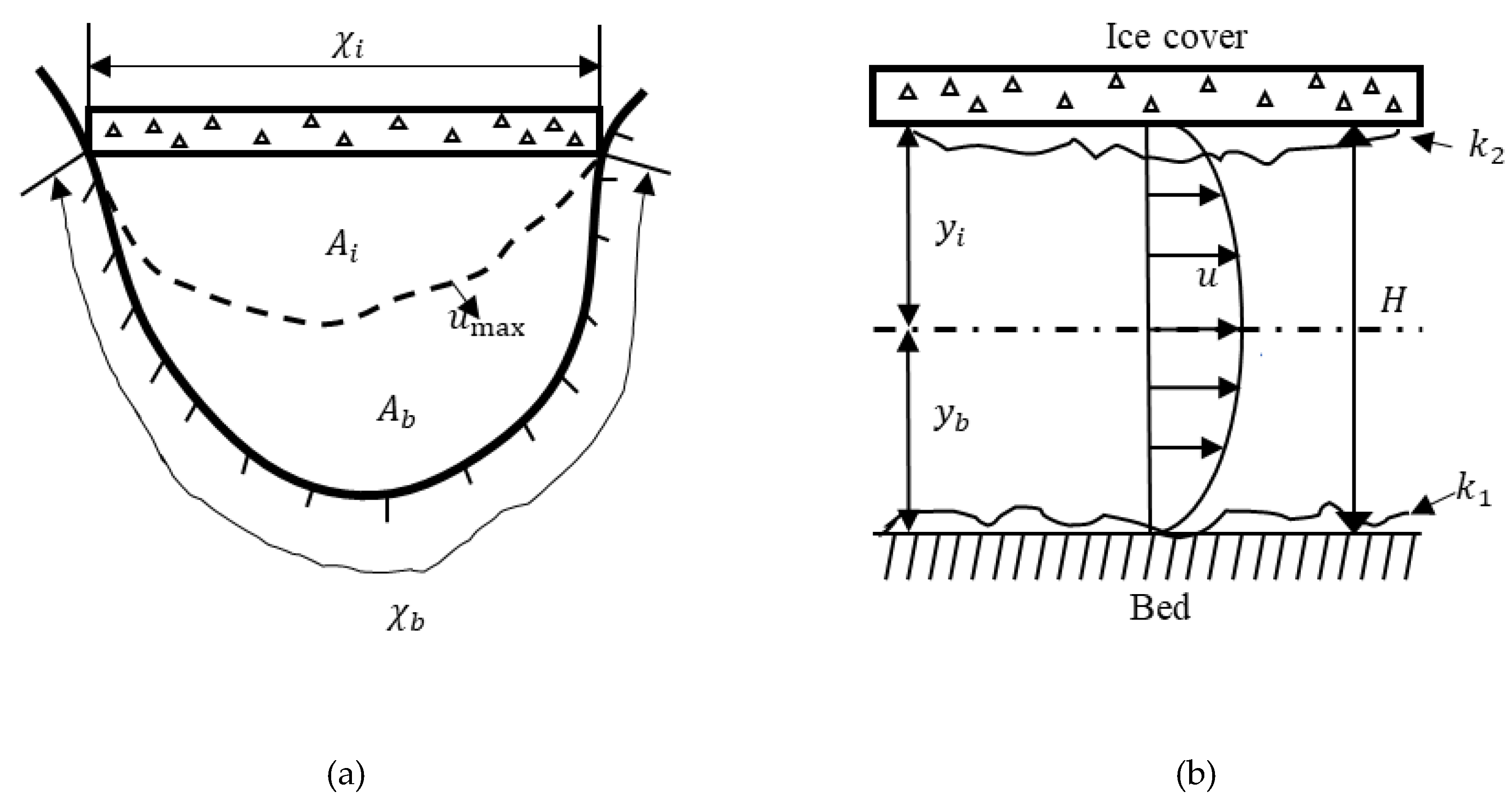
In Error! Reference source not found., is the total flow depth of the ice-covered channel, is the flow depth of the bed section, is the flow depth of the ice cover section, is the flow velocity, is the wetted perimeter of the ice cover section, is the wetted perimeter in the bed section, is the cross-sectional area of the ice cover section, is the cross-sectional area of the bed section.
Figure 1.
(a) Ice-covered channel's ice cover and bed sections (b) Velocity distribution in the ice-covered channel along the flow depth direction.
Figure 1.
(a) Ice-covered channel's ice cover and bed sections (b) Velocity distribution in the ice-covered channel along the flow depth direction.
2.2. General Resistance Formula for Ice-Covered Channels
According to the law of mass conservation, the total flow discharge in the channel equals the sum of the flow discharge in the ice cover section and the bed section
Where is the total flow discharge, is the flow discharge in the ice cover section, is the flow discharge in the bed section.
The hydraulic radius in the ice cover section and the bed section satisfies the relationship
Based on boundary conditions, it is known
By using Eq.(1) to express the flow discharge, we can derive
The total hydraulic radius can be expressed as
Where , is the ratio of the wetted perimeter in the bed section to that in the ice cover section, a dimensionless parameter.
Assuming , this assumption holds perfectly only when the flow is uniform. However, the flow in a frozen river may not be stable and uniform in fact. Despite this, many scholars still favor this assumption[23,24], and it has been extensively used in calculating the resistance of ice-covered channels.
From Eq.(3), Eq.(8) and Eq.(9), we can derive
By substituting Eq.(10) into Eq.(11), we get
Where , is the ratio of the hydraulic radius between the bed section and the ice cover section, a dimensionless parameter, , is the ratio of the Manning roughness between the ice cover section and the bed section, a dimensionless parameter.
If we assume i.e., the hydraulic radii of all sections are equal, by substituting into Eq.(12), we can obtain Lotter’s formulation14
If we assume , meaning the flow velocities of all sections are equal. Eq.(1) can be used to obtain
By substituting Eq.(14) into Eq.(12), we can derive Sabaneev's formulation17
If both assumptions of equal flow velocity and equal hydraulic radius are used, despite the serious issue that this leads to equal Manning’s roughness coefficients in the ice cover and bed sections, we can obtain Pavlovskiy’s formulation13
Based on the assumption of equal velocities, by adding the assumption that , we can obtain Sun Z’s formulation25
If we assume the channel is wide, meaning . and that the hydraulic radius of each section equals the flow depth of the respective section, substituting these assumptions into Eq.(12) yields Larsen’s formulation16
As discussed above, many resistance prediction formulas for ice-covered channels are simplifications of the general formula proposed in this study under specific assumptions. Eq.(12) provides a deeper explanation of the factors affecting resistance in ice-covered channels, which is significant for studying flow discharge in ice-covered channels.
2.3. Division of Regions in Ice-Covered Channels
The velocity of the channel is an important basis for studying sediment transport, river evolution, flow discharge, and other related issues26, By integrating the average flow velocity of the river, the transport capacity under specific flow depths can be computed. To derive the turbulent velocity distribution, Prandtl L. assumed (1) that the shear stress near the flow equals the wall shear stress, and (2) that the mixing length is proportional to the distance of the flow particle from the wall. In high Reynolds number flow, he derived the logarithmic velocity distribution formula for turbulent flow. However, this assumption has theoretical limitations, such as the need for fluid particles to pass through the mixing length before exchanging momentum with nearby particles, which contradicts the fact that momentum exchange occurs continuously as particles move. Additionally, when the logarithmic velocity distribution is applied to ice-covered channels, its inherent properties lead to discontinuities in the location of the maximum velocity point. Research[27,28,29,30] indicates that the logarithmic velocity distribution results in significant errors in the core flow area when describing the velocity distribution under the ice cover. When applying the logarithmic velocity distribution to describe flow beneath the ice cover, around 70% of the velocity distribution in the ice cover and bed sections aligns with the logarithmic distribution, but in about 30% of the area near the maximum velocity point, there is a significant discrepancy where the actual velocity is lower than the predicted value.
To address the issue of discontinuous velocity distribution in the theoretical model, Tsai and Ettema29, based on Odggard's research31, proposed using the two-power law to predict the velocity distribution under the ice cover, with two exponents representing the resistance in the ice cover and bed sections. The larger the value of the exponent, the smoother the boundary, and the smaller the flow resistance. Research by Chee and Haggag27, Teal29, and Li32 concluded that the two-power law can describe the continuous distribution of velocity with a single expression, avoiding the inherent flaws of the logarithmic velocity distribution law. Experiments and field observations indicate that the two-power law matches measurement data better[32,33] and facilitates the determination of the maximum velocity location, which has led to its application in research. The two-power law velocity distribution equation is
Where is the constant for the given flow velocity, and are the dimensionless parameters related to the bed and ice cover, and is the vertical depth. Teal et al. used over 22,300 vertical velocity profiles collected from 13 river flow measurement stations by the U.S. Geological Survey during the winter of 1988-1989, applying nonlinear regression methods. They estimated the exponent values to range from 1.5 to 8.5, with most values between 3 and 4. For open-channel flow, the exponent values range from 6 to 7.
The velocity gradient under the two-power law velocity distribution can be obtained from Eq.(19) as
Let , we can solve for the maximum velocity under the ice cover as
Where the maximum velocity occurs
Where is the depth where maximum velocity occurs, and , is the ratio of the exponents between the ice cover and bed sections.
2.4. New Predictor for Frozen River Estimation
By substituting Eq.(12) ino Eq.(1), we obtain
The research focuses on fully covered flow(), thus
Where is the width-to-depth ratio of the channel. If , then , which implies that the hydraulic radius of the flow section is half of the flow depth, a common assumption in wide channels.
Eq.(23) can be written as
Where is a physically based coefficient that indicates the correlation between the flow discharge of an ice−affected channel and that of an open−water channel. When the flow is converted to open−water flow, we easily find that . In this case, Eq.(25) simplifies to the Manning equation, indicating that the Manning equation is a special case with zero cover roughness34. By calculating the value of , the flow discharge of the ice-affected channel can be estimated using the stage-discharge curve established for open-water flow.
2.5. Estimation of Parameters
The Manning formula for steady, uniform flow in open channels is related to the Darcy-Weisbach coefficient through the following equation
Where is the Darcy-Weisbach resistance coefficient for the total flow cross-section,,and is the local gravitational acceleration. It is assumed that each section also satisfies a similar resistance relationship35.
Where and are the Darcy-Weisbach resistance coefficients for the bed and ice cover sections.
The relationship between the exponents and the Darcy-Weisbach resistance coefficients is described by36
where κ is the von Karman constant.
Therefore, we can obtain
From Eq.(8) and Eq.(9), we can obtain
Where is the velocity ratio between the ice cover section and the bed section.
From section2.3, we can get
From Eq.(35) and Eq.(36), we can obtain
If we continue the investigation, many interesting results can be found. Based on the previous discussion, the calculation process becomes relatively simple, and only the results are presented.
2.6. Estimation of and
In practical engineering, the flow cross-section of natural rivers is often simplified to a two-dimensional rectangular or trapezoidal shape, with geometric properties like channel width, flow depth, and slope easily measured directly. Based on the above basic information, the research provides three methods to estimate the exponents and .
- Given the velocity distribution along the cross-section, the regression method proposed by Attar and Li32 is applied to obtain the values;
- Given the Darcy-Weisbach resistance coefficients fb and fi, they can be estimated directly through Eq.(30) and Eq.(31);
- Given the Manning roughness coefficients nb and ni, by assuming an initial value of mb, iterative solutions are obtained using Eq.(10), Eq.(32), Eq.(33) and Eq.(37).
3. Results and Discussion
3.1. Verification of the Proposed Formula
3.1.1. Data Collection
The applicability of the proposed formula is verified using experimental data from fully covered channels, including 29 sets of laboratory measurements by Parthasarathy and Muste [34], Wei and Huang [35], Engmann [37], Smith and Ettema [38] and Zhang J [39] and 12 sets of field observations in natural river by Attar and Li [32] and Tatinclaux and Göğüs [40]. The geometric parameters and hydraulic conditions of the channel are listed in Error! Reference source not found..

Table 1.
Geometric parameters and hydraulic conditions used for validation.
| Data Sources | Runs | ||||||
|---|---|---|---|---|---|---|---|
| Smith and Ettema (1997) | SE-S2 | 0.912 | 1.37 | 0.181 | 4.51 | 7.56 | 0.0754 |
| SE-M2 | 0.912 | 1.29 | 0.195 | 4.79 | 5.72 | 0.0760 | |
| SE-R2 | 0.912 | 1.33 | 0.208 | 4.7 | 4.56 | 0.0756 | |
| SE-S4 | 0.912 | 1.34 | 0.182 | 4.59 | 7.69 | 0.0765 | |
| SE-M4 | 0.912 | 1.3 | 0.19 | 4.9 | 5.85 | 0.0755 | |
| SE-R4 | 0.912 | 1.3 | 0.209 | 4.7 | 4.56 | 0.0754 | |
| Tatinclaux and Gogus (1983) | TG-C1 | 425 | 0.5 | 5 | 5.73 | 2.44 | 1850 |
| TG-C2 | 425 | 0.5 | 4 | 5.47 | 2.44 | 1230 | |
| TG-C3 | 425 | 0.5 | 3.5 | 5.04 | 1.85 | 850 | |
| Parthasarathy and Muste (1994) | PM-R1 | 0.912 | 0.197 | 0.218 | 7.02 | 8.47 | 0.0501 |
| PM-R2 | 0.912 | 0.197 | 0.245 | 6.63 | 6.35 | 0.0501 | |
| PM-R3 | 0.912 | 0.197 | 0.29 | 5.73 | 4.75 | 0.0501 | |
| Wei and Huang (2002) | WH-Test 1 | 0.5 | 0.478 | 0.24 | 9.68 | 8.26 | 0.0501 |
| WH-Test 2 | 0.5 | 0.459 | 0.241 | 9.68 | 8.26 | 0.0501 | |
| WH-Test 3 | 0.5 | 0.446 | 0.242 | 9.68 | 8.26 | 0.0501 | |
| WH-Test 4 | 0.5 | 1.072 | 0.218 | 9.58 | 8.16 | 0.0699 | |
| WH-Test 5 | 0.5 | 1.124 | 0.199 | 9.48 | 8.08 | 0.0600 | |
| WH-Test 6 | 0.5 | 0.896 | 0.165 | 9.26 | 7.92 | 0.0401 | |
| WH-Test 7 | 0.5 | 0.774 | 0.144 | 9.26 | 7.92 | 0.0303 | |
| WH-Test 8 | 0.5 | 0.66 | 0.22 | 9.58 | 8.15 | 0.0507 | |
| WH-Test 10 | 0.5 | 2.845 | 0.192 | 8 | 3.15 | 0.0500 | |
| WH-Test 11 | 0.5 | 3.058 | 0.211 | 8 | 3.15 | 0.0602 | |
| WH-Test 12 | 0.5 | 2.526 | 0.201 | 8 | 3.15 | 0.0502 | |
| WH-Test 13 | 0.5 | 2.534 | 0.201 | 8 | 3.15 | 0.0502 | |
| WH-Test 15 | 0.5 | 2.572 | 0.236 | 3.45 | 3.04 | 0.0507 | |
| WH-Test 16 | 0.5 | 2.277 | 0.217 | 3.45 | 3.04 | 0.0412 | |
| J Zhang(2021) | Case1 | 1 | 1 | 0.15 | 6.35 | 4.84 | 0.0536 |
| Case2 | 1 | 1 | 0.185 | 7.13 | 5.31 | 0.0783 | |
| Engmann (1977) | EN-101 | 1.22 | 0.65 | 0.0497 | 3.1 | 6.46 | 0.0071 |
| EN-102 | 1.22 | 0.79 | 0.0649 | 4.12 | 8.08 | 0.0156 | |
| EN-103 | 1.22 | 2.49 | 0.0384 | 4.6 | 7.54 | 0.0127 | |
| EN-104 | 1.22 | 1.61 | 0.0396 | 4.6 | 7.54 | 0.0114 | |
| Attar and Li (2012) | S.W. Miramichi R., NB | 92 | 0.07 | 2 | 3.59 | 7.39 | 51 |
| Burnt R., ON | 32 | 0.04 | 1.9 | 3.2 | 5.48 | 10 | |
| Pembina R., AB | 74 | 0.13 | 0.7 | 3.23 | 6.25 | 12 | |
| Halfway R., BC | 39 | 0.8 | 0.54 | 2.77 | 5.96 | 7.4 | |
| Peace R., NWT | 525 | 0.04 | 4.5 | 5.44 | 9.22 | 1111 | |
| Yellowknife R., NWT | 72 | 0.01 | 3 | 3.55 | 5.92 | 24 | |
| Fraser R., BC | 95 | 0.1 | 1.3 | 3.25 | 6.37 | 32 | |
| Takhini R. YT | 46 | 0.08 | 1.4 | 3.12 | 5.96 | 14 | |
| Yukon R., YT | 145 | 0.4 | 2.5 | 3.69 | 7.06 | 246 |
3.1.2. Model Verifications
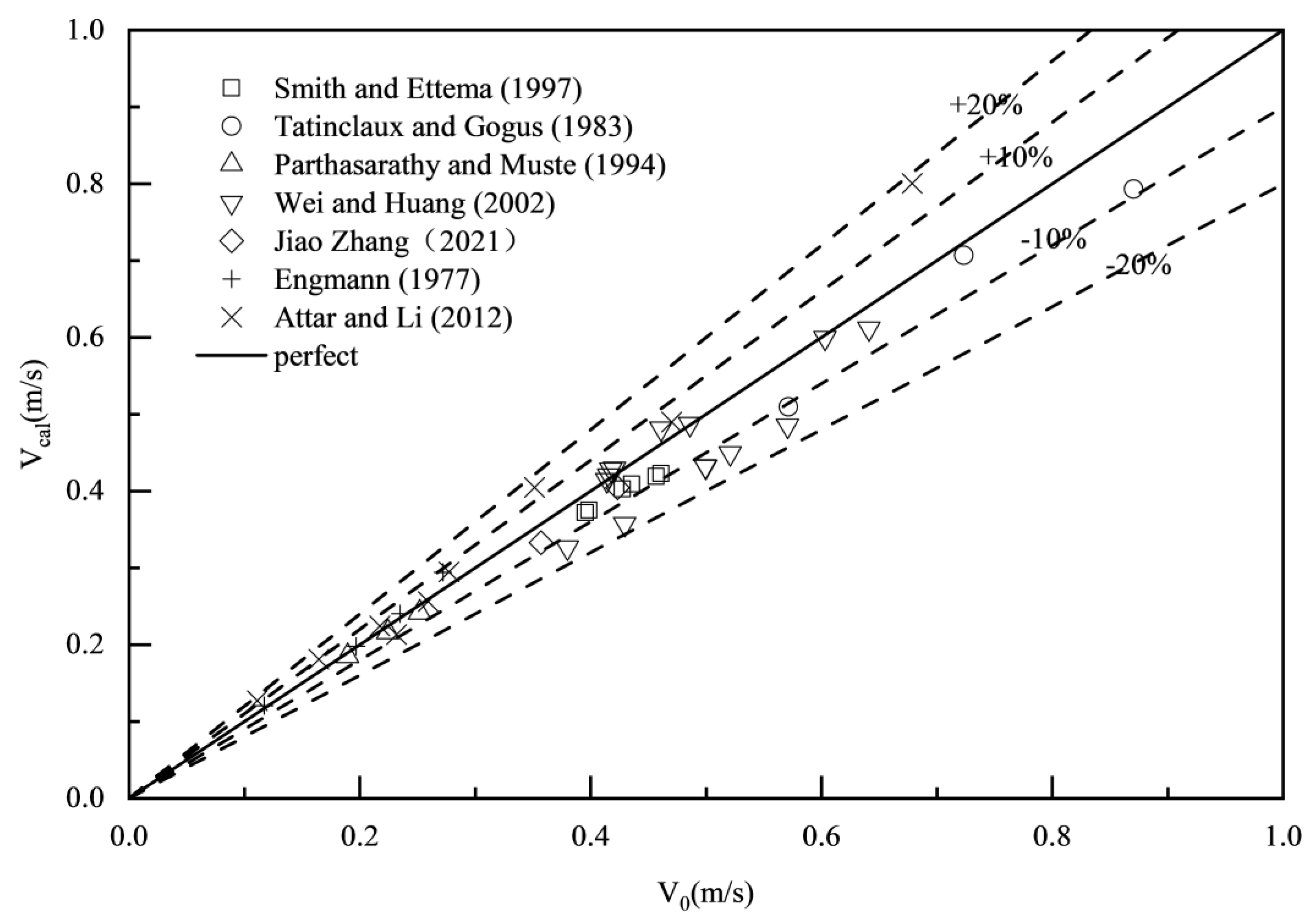
The proposed Eq.(23) is compared with the flow discharge results calculated using the traditional Lotter, Sabaneev, Larsen, and Pavlovskiy formulas. Since there are significant differences in flow discharge under different conditions, velocity errors are used instead of flow discharge for comparison. The percentage error in velocity is equal to the percentage error in flow discharge, making this substitution method valid. We use the relative error to evaluate the performance of each formula.
Where is the number of all verified conditions), is the calculated velocity, is the measured velocity.
The comparison of the measured velocity results with the actual values shows that the average error of the proposed formula Eq.(23) is 3.97%, with a maximum error of 15.08% and a minimum error of 0.31%, shown in Error! Reference source not found.; for the Lotter formula, the average error is 16.35%, the maximum error is 55.55%, and the minimum error is 0.31%, shown in Error! Reference source not found.; for the Sabaneev formula, the average error is 5.23%, the maximum error is 15.94%, and the minimum error is 0.40%, shown in Error! Reference source not found.; for the Larsen formula, the average error is 5.89%, the maximum error is 20.93%, and the minimum error is 0.18%, shown in Error! Reference source not found.; for the Pavlovskiy formula, the average error is 6.82%, the maximum error is 17.97%, and the minimum error is 0.11%, shown in Error! Reference source not found.. Compared to traditional formulas, the proposed formula Eq.(23) not only accurately predicts the flow discharge in ice-covered channels, but also shows a significant improvement in performance.
Figure 2.
Comparison of estimated results of Eq.(23) with the measured data.

Figure 3.
Comparison of estimated results of the Lotter formula with the measured data.
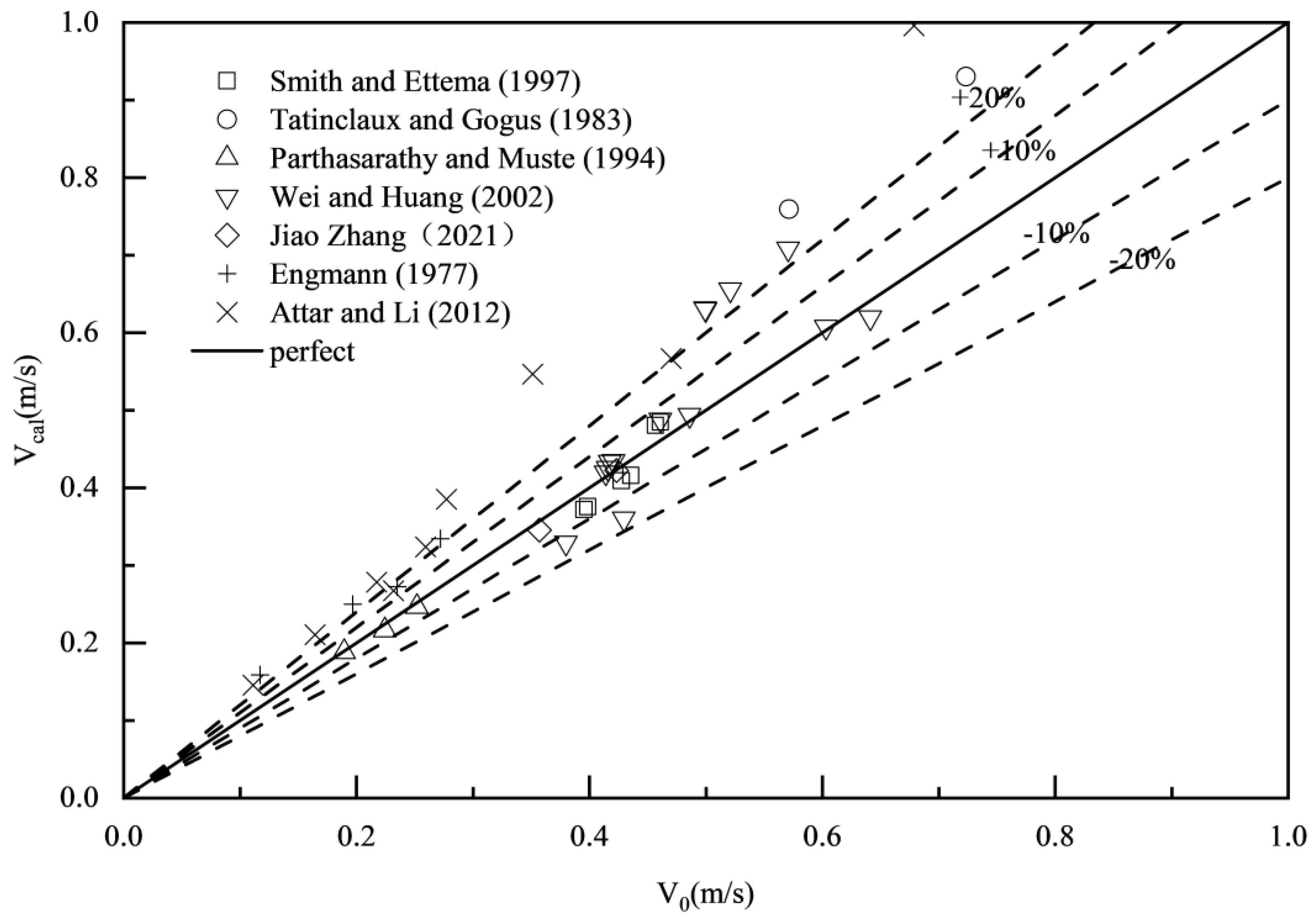
Figure 4.
Comparison of estimated results of the Sabaneev formula with the measured data.
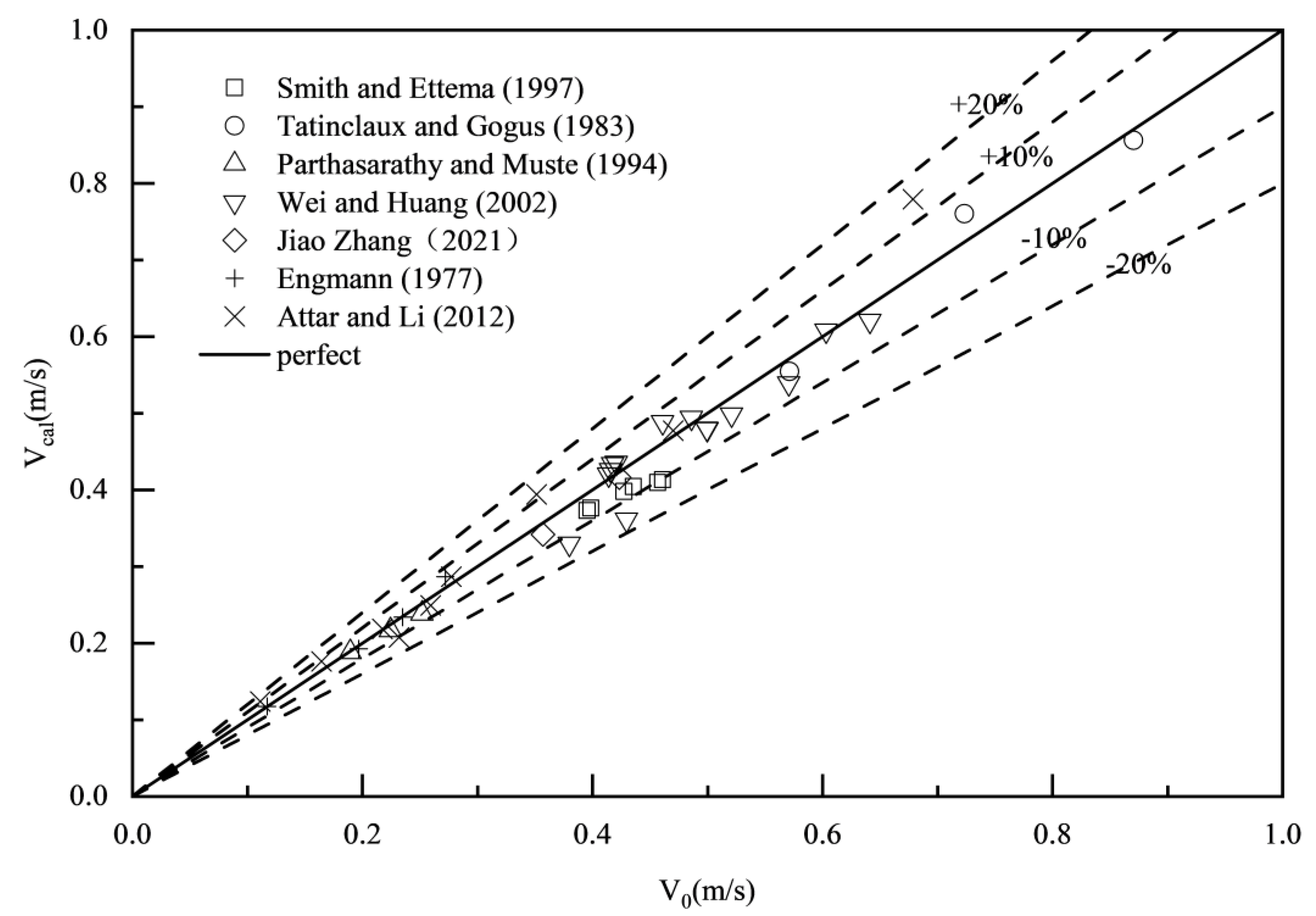
Figure 5.
Comparison of estimated results of the Larsen formula with the measured data.
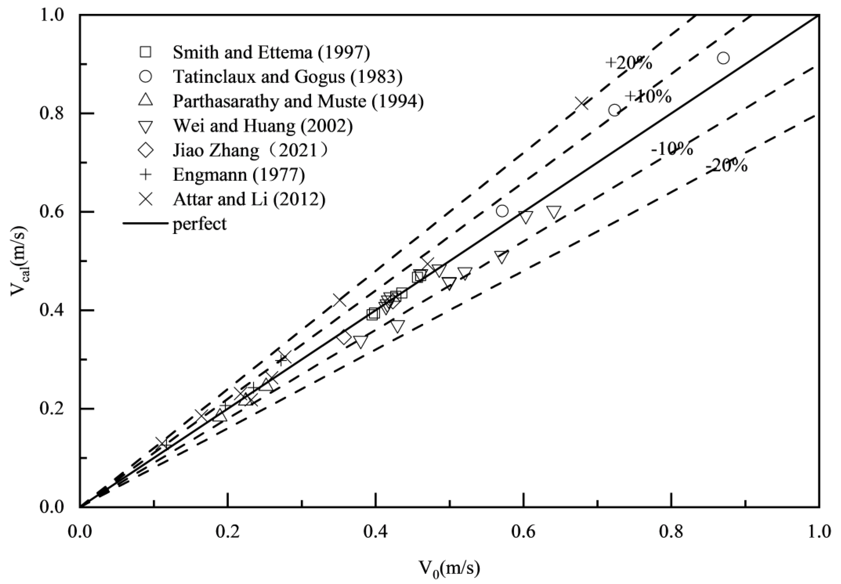
Figure 6.
Comparison of estimated results of the Pavlovskiy formula with the measured data.
3.2. Hydraulic Radius
It is widely assumed in past calculations of resistance in ice-covered channels that the hydraulic radius of the sections are equal, i.e., . This assumption does not reflect reality, as it leads to the conclusion that the ice cover roughness and bed roughness are nearly equal, which is obviously contradictory. As shown in Error! Reference source not found., in the given channel , there is a negative correlation between the hydraulic radius of the ice cover section and that of the bed section, and the total hydraulic radius is between the two. Studies indicate that in the vast majority of cases, the difference between the hydraulic radius of the ice cover section and the bed section and the total hydraulic radius exceeds 10%, and sometimes even exceeds 30%, making the assumption unreasonable.
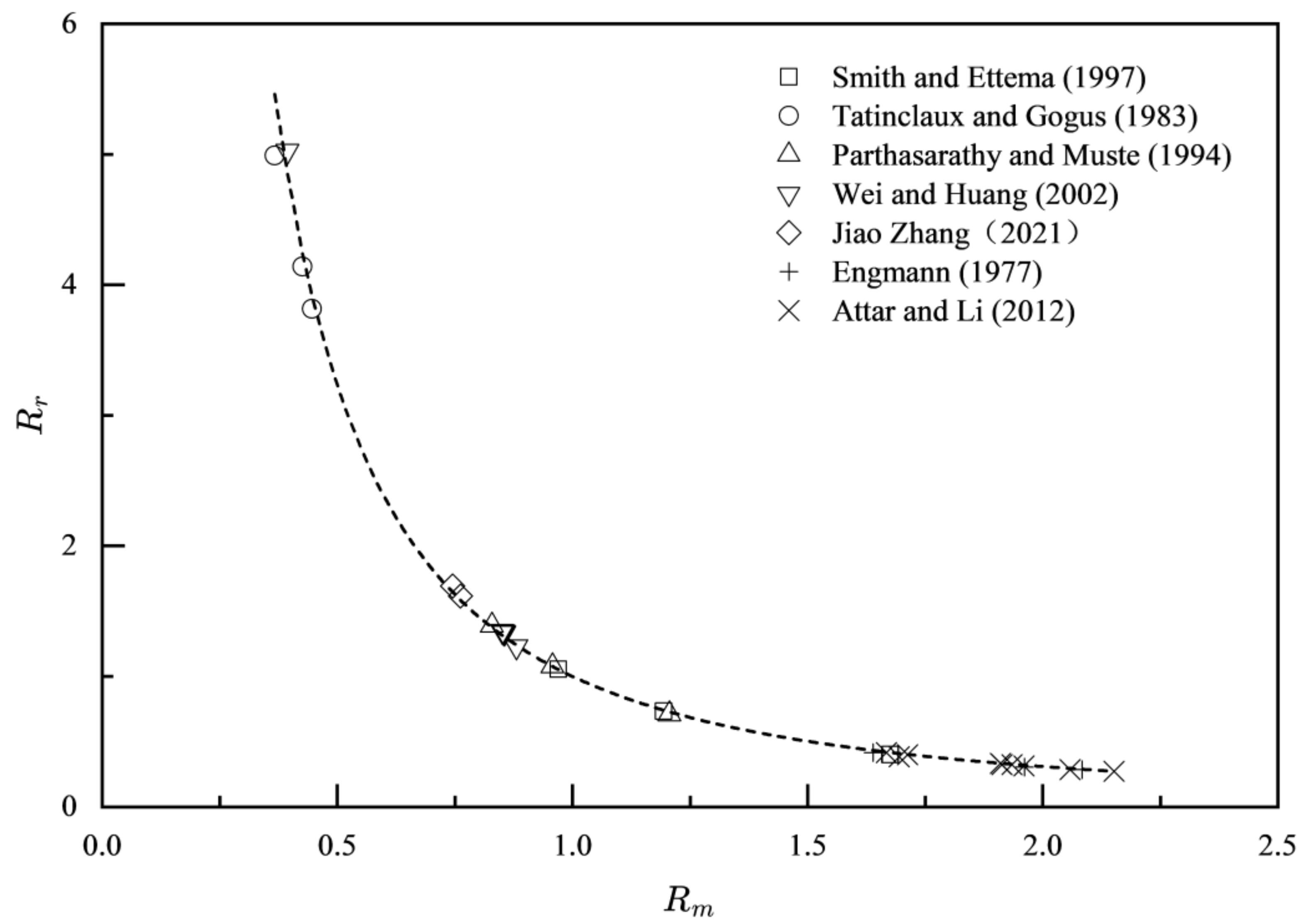
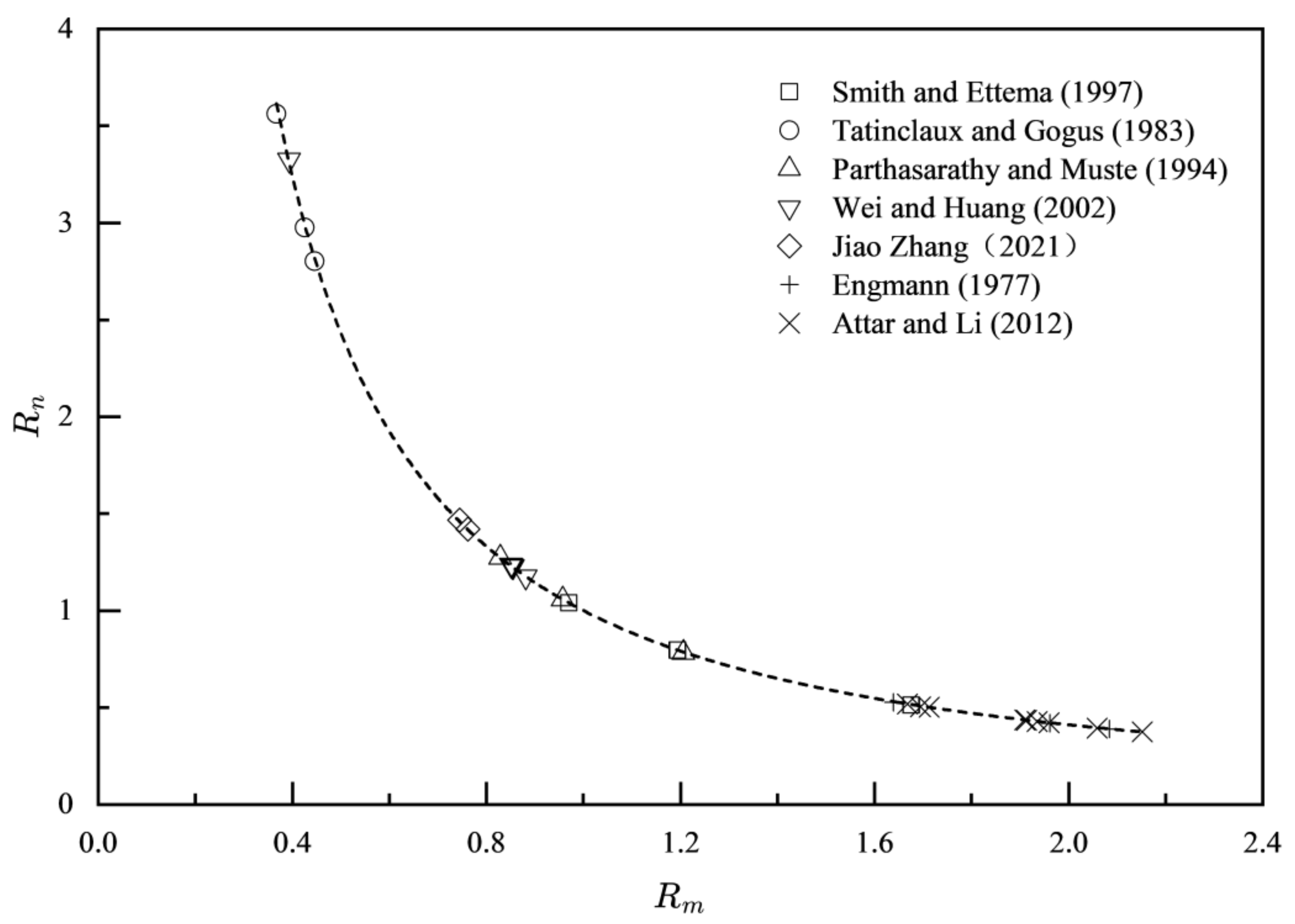
Error! Reference source not found. shows the trend of as varies. The result shows that the Pearson correlation coefficient between the hydraulic radius ratio and the exponent ratio is , indicating a strong negative correlation. Based on the data, we use a function to fit and and evaluate the fitting curve with the Coefficient of Determination (COD) and Standard Error (SE) indicators.
Where . Eq.(40) provides a simple method for calculating the Manning roughness or the exponent.
Figure 7.
(a) Comparison of , and (b) Magnified view of local details.
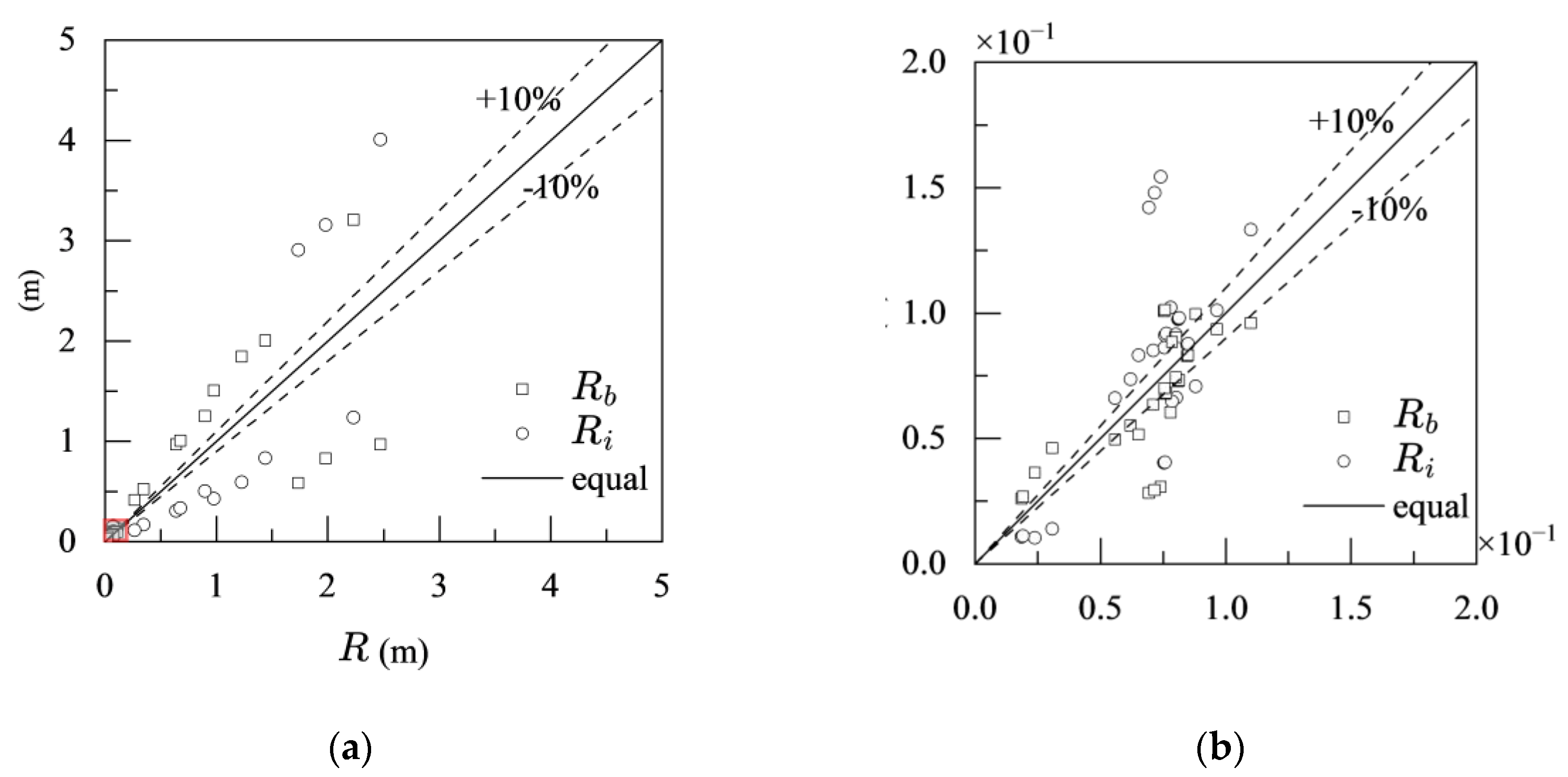
Figure 8.
Variations of and
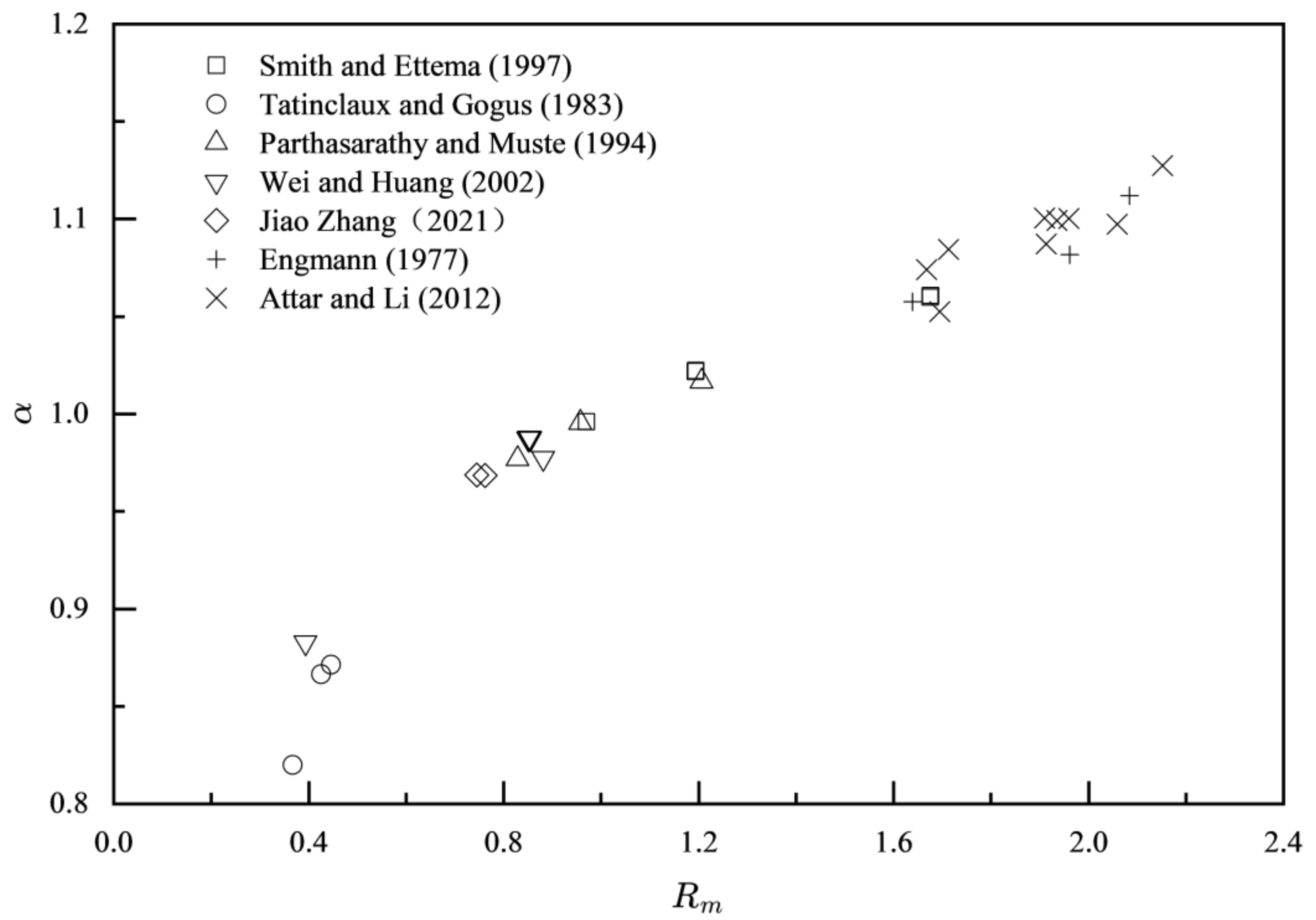
3.3. Velocity
The assumption of equal average velocity across sections is widely favored by researchers studying ice-covered channels[41,42,43]. According to the results of the study, the assumption of equal velocity across sections is not suitable, as the average velocity in each section is greatly influenced by the roughness of that section.
Error! Reference source not found. shows the relationship between and . The results show a positive correlation between and . In the validation data, values typically range from 0.9 to 1.1, suggesting that the assumption of equal velocity causes a 5% to 10% error in most cases. only when the ice cover roughness is equal to the bed roughness. The research advises against using the assumption of equal velocity to calculate flow discharge during the initial freezing stage of ice-affected channels in winter, as the large difference in roughness between the ice cover and bed would lead to large errors.
Figure 9.
Variations of and
3.4. Manning Resistance Coefficient
Teal29 pointed out that the larger the exponent, the smoother the boundary and the lower the flow resistance. In previous studies44, Eq.(14) was used to estimate flow resistance, and as discussed in Section 2.2, this simplified formula is based on the assumption of equal velocity. Section 3.3 demonstrates that the equal velocity assumption carries some degree of error, especially when the roughness difference between the ice cover and bed sections is significant. Therefore, the research delves further into the relationship between Manning's roughness, the exponents, and hydraulic radius. As shown in Error! Reference source not found., and display a distinct negative correlation, with a Pearson correlation coefficient of . By fitting the curve, we derived
Where .
By combining Eq.(40) and Eq.(41), we deduced
Figure 10.
Variations of and
3.5. Two Simplified Formulas for Flow Prediction
By substituting the results of Section 3.2 and Section 3.4 into Eq.(23), the research derived two simplified formulas for flow prediction.
Where and are empirical parameters, with the recommended values are,.
Where and are empirical parameters, with the recommended values are and .
Compared with measured data, the average error of the proposed formula Eq.(43) is 4.20%, with a maximum error of 15.17% and a minimum error of 0.23%, shown in Error! Reference source not found.; the average error of the proposed formula Eq.(44) is 4.16%, with a maximum error of 14.93% and a minimum error of 0.49%, shown in Error! Reference source not found.. The two simplified formulas, while maintaining high computational accuracy, greatly reduce the labor costs and time required for measurements and calculations in practical engineering, providing operators with more options to calculate flow discharge in ice-covered channels. For example, using the channel resistance before freezing to replace the bed resistance after freezing, or using methods to measure roughness height for estimating roughness, or measuring the exponents of velocity distribution, etc. Hence, we highly recommend using Eq.(43) or Eq.(44) to calculate flow discharge in ice-covered channels in practical engineering.
Figure 11.
Comparison of estimated results of Eq.(43) with the measured data.

Figure 12.
Comparison of estimated results of Eq.(44) with the measured data.

3.6. Shortcomings
The assumption of equal energy slopes in each section, as used by Larsen, P. A16 and Ashton, G. D45, essentially assumes that the flow under the ice cover is uniform, which is also adopted in this study. However, the flow in natural rivers is quite complex, and may not always form a stable uniform flow. The energy slope in the bed section is often smaller than that in the ice cover section46, which may negatively affect the accuracy of the research. While field measurements suggest the results are trustworthy, the data sample is limited, requiring more field data for validation.
Eq.(43) and Eq.(44) rely on the determination of empirical parameters, the research provides optional values, but more field data is needed in the future to determine the range of the parameters.
4. Conclusions
The research derives a flow discharge calculation equation for ice-covered channels based on physical conditions and provides two simple formulas, which can easily estimate the flow discharge in ice-covered channels. The analysis results are in strong agreement with laboratory measurements and field observations, showing that the formulas proposed in this study can be effectively used for flow discharge prediction in ice-covered channels. The main conclusions are as follows
- Assuming equal flow velocity or equal hydraulic radius in each section leads to errors in predicting resistance or flow discharge in ice-covered channels, especially the latter, which may result in unacceptable errors.
- Compared to commonly used traditional formulas, such as the Lotter formula, Sabaneev formula, Larsen formula, and Pavlovskiy formula, the general formula and two simplified formulas proposed in the research exhibit superior performance. It is recommended to use the methods or simplified formulas presented in the research for more accurate flow discharge prediction.
Author Contributions
Conceptualization, H.Z. and Z.M.; methodology, H.Z.; formal analysis, H.Z.; data curation, H.Z.; writing—original draft preparation, H.Z.; writing—review and editing, H.Z.; supervision, Z.M.; All authors have read and agreed to the published version of the manuscript.
Funding
This research received no external funding.
Data Availability Statement
Data are contained within the article.
Acknowledgments
We thank everyone who helped us during the completion of the thesis. We also thank the reviewers for their useful comments and suggestions.
Conflicts of Interest
The authors declare no conflicts of interest.
References
- Hou, Z.; Zhao, J.; Wang, Q.; et al. Discriminant analysis of the freeze-up and break-up conditions in the Inner Mongolia Reach of the Yellow River [J]. Journal of Water and Climate Change 2023, 14, 3166–3177. [Google Scholar] [CrossRef]
- Morse, B.; Hicks, F. Advances in river ice hydrology 1999–2003 [J]. Hydrological Processes: An International Journal 2005, 19, 247–263. [Google Scholar] [CrossRef]
- Chokmani, K.; Ouarda, T.B.M.J.; Hamilton, S.; et al. Comparison of ice-affected streamflow estimates computed using artificial neural networks and multiple regression techniques [J]. Journal of Hydrology 2008, 349, 383–396. [Google Scholar] [CrossRef]
- Liu, C.K.; Ma, R.; Qiu, X.; et al. Multi-scale simulation on joint operation of reservoir groups for flood control based on 3D GIS [J]. Yangtze River 2021, 52, 212–216. [Google Scholar]
- Shen, H.T.; Harden, T.O. The effects of ice cover on vertical transfer streamwise channels [J]. Water Resources Bulletin 1978, 14, 1112–1131. [Google Scholar] [CrossRef]
- Walker, J.F.; Wang, D. Measurement of flow under ice cover in North America [J]. Journal of Hydraulic Engineering, ASCE 1997, 123, 1037–1040. [Google Scholar] [CrossRef]
- Majewski, W. Flow in open channels under the influence of ice cover [J]. Acta Geophysica 2007, 55, 11–22. [Google Scholar] [CrossRef]
- Chai, Y.F.; Deng, J.Y.; Yang, Y.P.; et al. Evolution characteristics and driving factors of the water level at the same discharge in the Jingjiang reach of Yangtze River [J]. Acta Geographica Sinica 2021, 76, 101–113. [Google Scholar]
- Duan, W.G.; Xing, M.Y.; Huang, M.H.; Yang, J.B.; Sha, J.T. Observation and analysis of ice cover roughness in the South-to-North Water Diversion Middle Route Project [J]. Journal of Yangtze River Scientific Research Institute 2024, 41, 78–85. [Google Scholar]
- Hanjalić, K.; Launder, B.E. Fully developed asymmetric flow in a plane channel [J]. Journal of Fluid Mechanics 1972, 51, 301–335. [Google Scholar] [CrossRef]
- Fu, H.; Guo, X.; Yang, K.; et al. Distribution of vertical flow velocity upstream of an inverted siphon in the Middle Route of South-to-North Water Diversion Project [J]. Advances in Water Science 2017, 28, 922–929. [Google Scholar]
- Walker, J.F. Accuracy of selected techniques for estimating ice-affected streamflow [J]. Journal of Hydraulic Engineering 1991, 117, 697–712. [Google Scholar] [CrossRef]
- Pavlovsky, N.N. On a design formula for uniform movement in channels with nonhomogeneous walls [J]. Transactions of All-Union Scientific Research Institution of Hydraulic Engineering 1931, 3, 157–164. [Google Scholar]
- Lotter, G.K. Considerations on hydraulic design of channels with different roughness of walls [J]. Transactions, All-Union Scientific Research Institute of Hydraulic Engineering, Leningrad 1933, 9, 238–241. [Google Scholar]
- Einstein, H.A. Method of calculating the hydraulic radius in a cross section with different roughness [C]//Trans ASCE, 1942.
- Larsen, P.A. Head losses caused by an ice cover on open channels [J]. Journal of the Boston Society of Civil Engineers 1969, 56, 45–67. [Google Scholar]
- Sabaneev, A.A. On the computation of a uniform flow in a channel with nonuniform walls: Leningrad Polytech. Inst [J]. Trans, 1948 (5).
- Uzuner, M.S. The composite roughness of ice-covered streams [J]. Journal of Hydrological Research 1975, 13, 79–102. [Google Scholar] [CrossRef]
- Te Chow, V. Open channel hydraulics [M]. 1959.
- Yen, B.C. Dimensionally homogeneous Manning's formula [J]. Journal of hydraulic engineering 1992, 118, 1326–1332. [Google Scholar] [CrossRef]
- Tang TC, C.; Davar, K.S. Resistance to flow in partially-covered channels [M]. Fredericton, Canada: University of New Brunswick, 1985.
- Tian, F.; Yuan, X.; Wang, X.; et al. Review on disaster prevention fractal theory of nonlinear dynamic system in rivers (networks) at home and abroad [J]. J. Hydraul. Eng 2018, 49, 926–936. [Google Scholar]
- Beltaos, S.; Tang, P.; Rowsell, R. Ice jam modelling and field data collection for flood forecasting in the Saint John River, Canada [J]. Hydrological Processes 2012, 26, 2535–2545. [Google Scholar] [CrossRef]
- Li, S.S. Estimates of the Manning's coefficient for ice-covered rivers [C]//Proceedings of the Institution of Civil Engineers-Water Management. Thomas Telford Ltd 2012, 165, 495–505. [Google Scholar]
- Sun, Z.; Sui, J. Calculation of water level in a river reach with frazil ice jam [C]//Proc., IAHR Symp. 1990: 756-765.
- Bonakdari, H. Establishment of relationship between mean and maximum velocities in narrow sewers [J]. Journal of environmental management 2012, 113, 474–480. [Google Scholar] [CrossRef] [PubMed]
- Chee, S.P.; Haggag MR, I. Flow resistance of ice-covered streams [J]. Canadian Journal of Civil Engineering 1984, 11, 815–823. [Google Scholar] [CrossRef]
- Lau, Y.L. Velocity distributions under floating covers [J]. Canadian Journal of Civil Engineering 1982, 9, 76–83. [Google Scholar] [CrossRef]
- Teal, M.J.; Ettema, R.; Walker, J.F. Estimation of mean flow velocity in ice-covered channels [J]. Journal of Hydraulic Engineering 1994, 120, 1385–1400. [Google Scholar] [CrossRef]
- Dolgopolova, E.N. Velocity distribution in ice-covered flow [C]//Ice in surface waters: proceedings of the 14th international symposium on ice, New York, 27-31 July 1998. Volume 1. 1998: 123-129.
- Odgaard, A.J. River-meander model. I: Development [J]. Journal of Hydraulic Engineering 1989, 115, 1433–1450. [Google Scholar] [CrossRef]
- Attar, S.; Li, S.S. Data-fitted velocity profiles for ice-covered rivers [J]. Canadian Journal of Civil Engineering 2012, 39, 334–338. [Google Scholar] [CrossRef]
- Healy, D.; Hicks, F.E. Index velocity methods for winter discharge measurement [J]. Canadian Journal of Civil Engineering 2004, 31, 407–419. [Google Scholar] [CrossRef]
- Parthasarathy, R.N.; Muste, M. Velocity measurements in asymmetric turbulent channel flows [J]. Journal of Hydraulic Engineering 1994, 120, 1000–1020. [Google Scholar] [CrossRef]
- Wei, L.Y.; Huang, J.Z. Composite manning roughness coefficient of ice-covered flow [J]. Engineering Journal of Wuhan University 2002, 35, 1–8. [Google Scholar]
- Chen, G.; Zhou, M.; Gu, S.; et al. Analytical model for stage-discharge prediction in rectangular ice-covered channels [J]. Journal of hydraulic engineering 2016, 142, 06016006. [Google Scholar] [CrossRef]
- Engmann, E.O. Turbulent diffusion in channels with a surface cover [J]. Journal of Hydraulic Research 1977, 15, 327–335. [Google Scholar] [CrossRef]
- Smith, B.T.; Ettema, R. Flow resistance in ice-covered alluvial channels [J]. Journal of hydraulic engineering 1997, 123, 592–599. [Google Scholar] [CrossRef]
- Zhang, J.; Wang, W.; Li, Z.; et al. Analytical models of velocity, reynolds stress and turbulence intensity in ice-covered channels [J]. Water 2021, 13, 1107. [Google Scholar] [CrossRef]
- Tatinclaux, J.C.; Gogus, M. Asymmetric plane flow with application to ice jams [J]. Journal of Hydraulic Engineering 1983, 109, 1540–1554. [Google Scholar] [CrossRef]
- Komora, J.; Sumbal, J. Head losses in channels with ice cover [C]//Proc. 12th Congress of the Int. Assoc. for Hydraul. Res. 1967, 4, 270–274. [Google Scholar]
- Secil Uzuner, M. The composite roughness of ice covered streams [J]. Journal of Hydraulic Research 1975, 13, 79–102. [Google Scholar] [CrossRef]
- Carey, K.L. Observed configuration and computed roughness of the underside of river ice, St. Croix River, Wisconsin [J]. US Geological Survey Professional Paper 1966, 550. [Google Scholar]
- Beltaos, S. River ice jams: Theory, case studies, and applications [J]. Journal of Hydraulic Engineering 1983, 109, 1338–1359. [Google Scholar] [CrossRef]
- Ashton, G.D. River and lake ice engineering [M]. Water Resources Publication, 1986.
- Ghareh Aghaji Zare, S.; Moore, S.A.; Rennie, C.D.; et al. Estimation of composite hydraulic resistance in ice-covered alluvial streams [J]. Water Resources Research 2016, 52, 1306–1327. [Google Scholar] [CrossRef]
Disclaimer/Publisher’s Note: The statements, opinions and data contained in all publications are solely those of the individual author(s) and contributor(s) and not of MDPI and/or the editor(s). MDPI and/or the editor(s) disclaim responsibility for any injury to people or property resulting from any ideas, methods, instructions or products referred to in the content. |
© 2025 by the authors. Licensee MDPI, Basel, Switzerland. This article is an open access article distributed under the terms and conditions of the Creative Commons Attribution (CC BY) license (http://creativecommons.org/licenses/by/4.0/).
Copyright: This open access article is published under a Creative Commons CC BY 4.0 license, which permit the free download, distribution, and reuse, provided that the author and preprint are cited in any reuse.


