1. Introduction
In the evolving landscape of predictive analytics, high-dimensional time-series data, prevalent across various domains such as finance, healthcare, and engineering, presents significant challenges and opportunities for predictive modelling [
1,
2]. The development of sophisticated predictive models has become increasingly crucial due to the rising complexity and volume of such data [
3]. The advancement of predictive algorithms has been particularly impactful in fields where accurate and timely predictions can lead to substantial benefits, including financial gain, improved decision-making, resource allocation, and risk mitigation [
1]. Domains such as climate modelling, energy consumption forecasting, and biomedical signal processing are increasingly influenced by rapid advancements in computational techniques [
2]. The ability to forecast future trends with high accuracy is essential for researchers, practitioners, and policymakers, as it enables better planning and strategy development [
4]. These areas demand advanced analytical strategies that can accurately predict future states and adapt to rapid changes in dynamic conditions [
1].
Recent research in time-series forecasting has extensively explored various predictive models, ranging from simple methods such as traditional linear regressions and autoregressive models to more sophisticated machine learning and deep learning techniques [
2]. These methodologies have demonstrated significant potential in handling the nonlinear patterns typical in complex time-series data, which critically depend on the accurate selection of influential parameters affecting dynamic behaviours [
3]. To this end, current research has extensively utilised innovative deep learning architectures, including hybrid models and Transformer-based networks [
1,
4]. These technologies have markedly enhanced prediction accuracy by effectively harnessing large datasets and capturing intricate temporal dependencies and feature interactions [
1].
Despite significant advancements in forecasting methodologies, a noticeable gap persists in effectively determining the optimal amount of historical data that should be considered for accurate predictions [
3]. This aspect, typically addressed through the concept of
sliding window sizes, is critical because the choice of window size directly influences a model’s adaptability and its capacity to effectively capture and respond to relevant trends and anomalies – a topic that remains inadequately explored [
2]. Predominantly, existing approaches rely on fixed window sizes, often chosen arbitrarily, which fail to align with the dynamic nature of many real-world processes and can lead to significant inaccuracies in predictive outcomes [
1]. The selection of an appropriate window size is paramount, as it determines the model’s ability to learn from past trends and adapt to new developments, balancing the need to capture sufficient historical context without diluting the relevance of the most recent data [
4]. Therefore, the development of dynamic window sizing strategies capable of adjusting in real-time to changes in data patterns is not just beneficial but essential [
3]. Such strategies enhance not only the predictive accuracy but also the overall reliability of time-series forecasting models, addressing the critical need for models that can balance historical context with the acuity of recent data [
2].
To address this challenge, this work employs cryptocurrency markets as a case study due to their inherent high volatility and complex dynamics [
1]. The unpredictable nature of cryptocurrency time-series data provides an ideal environment for evaluating advanced predictive methodologies [
4]. By analysing cryptocurrency data, this study leverages state-of-the-art machine learning algorithms to identify optimal window sizes corresponding to different levels of market volatility [
3]. These optimal window sizes are then integrated to develop dynamic window sizing techniques that enhance the adaptability and accuracy of predictive models [
2]. This research aims to address the aforementioned gaps by introducing an innovative approach to window size optimisation across a variety of cryptocurrencies, allowing models to adjust their parameters in real time based on current data characteristics [
1]. The significance of this research is underscored by the critical need for robust, adaptive models that can handle the unpredictable nature of complex time-series data [
4]. By presenting this novel approach to window size optimisation, the study contributes to theoretical advancements in time-series forecasting and offers practical tools that can significantly improve decision-making in various domains [
2].
The benefits of this research are demonstrated through comprehensive experiments, comparing the performance of dynamically adjusting models against traditional static models [
3]. The dynamic models are evaluated based on accuracy and error metrics and are further assessed through actual predictions under varying data conditions [
1]. The results indicate that dynamic window sizing models outperform traditional static models, particularly in terms of prediction accuracy and responsiveness to changes in data patterns [
4]. These findings suggest that this methodology could set a new benchmark in predictive analytics for time-series forecasting [
2].
This introduction establishes the foundation for the subsequent sections of this work. It leads into an in-depth exploration of related literature, detailing the current state of research and introducing the novel methodologies developed within this investigation. The following methodology section outlines the strategies employed to dynamically optimise window sizes in time-series predictions, aiming to improve both the accuracy and responsiveness of forecasting models to changing data patterns. Subsequent sections provide a thorough examination of the data collection methods, experimental design, optimisation processes, and model development, as well as the performance metrics for these models. This systematic approach is followed by the presentation and discussion of the results, which assess the impact of dynamic window sizing on model performance, providing key insights and exploring the broader implications of these findings within the field of time-series forecasting.
1.1. Contributions
Emerging from the critical evaluation of current methodologies and the outlined objectives for this study, several key research questions/contributions have been formulated to guide the subsequent investigation.
- 1.
Correlation of Window Size with Model Performance and Volatility: This study systematically evaluates the relationship between window size and model performance across varying levels of market volatility. By establishing a clear correlation, the research identifies optimal window sizes that maximise predictive accuracy, tailored to specific volatility conditions.
- 2.
Development and Implementation of a Dynamic Window Sizing Framework: Building on the identification of optimal window sizes, this research introduces a dynamic window sizing framework that adjusts window sizes in real time based on current market fluctuations. The implementation demonstrates significant improvements in predictive accuracy over static window sizing approaches, providing a robust and adaptive solution for time-series forecasting.
- 3.
Comprehensive Comparative Analysis of Dynamic vs. Static Models: This research presents a thorough comparison between the dynamic window sizing model and traditional static window-size models, assessing them using metrics such as MSE, MAE, RMSE, and F1 score. The analysis demonstrates the dynamic model’s superiority in handling volatile cryptocurrency markets, establishing it as a more effective approach for time-series forecasting.
By addressing these questions, the research aims to contribute novel insights and methodologies to the field of financial forecasting, specifically within the context of cryptocurrency markets. The outcomes of this study are expected to provide significant advancements in both the theoretical understanding and practical applications of time-series forecasting models.
2. Related Work
Time-series forecasting in financial markets is a sequence-dependent analytical process where prediction accuracy relies on comprehending historical trends and data patterns. This sequential nature necessitates in-depth analysis of past behaviours to predict future outcomes. Accurately identifying influential parameters and selecting appropriate algorithms are crucial for enhancing the precision and reliability of predictive models, especially in volatile cryptocurrency markets. In this context, determining the optimal window size is fundamental, as it defines the length of historical data the models analyse, directly influencing their ability to recognize relevant patterns and adapt to rapid market changes.
2.1. In-Depth Analysis of Key Research
The adoption of advanced deep learning algorithms and integration of diverse data sources have significantly evolved the field of cryptocurrency price prediction, enhancing the accuracy and robustness of predictive models crucial for volatile markets. This section reviews pivotal studies that have established current paradigms and methodologies, highlighting key approaches and findings that have improved forecasting accuracy and facilitated optimal model configurations. Central to this discussion is the dynamic optimisation of window sizes, a critical factor in both cryptocurrency-specific and general financial time-series forecasting. The importance of adaptive strategies in window size determination is underscored, emphasising how these strategies enhance model responsiveness and predictive performance in highly fluctuating market conditions.
2.1.1. Algorithmic Models in Cryptocurrency Forecasting
Cryptocurrency price prediction has been a focus for researchers aiming to decipher market trends and price movements through the application of advanced machine learning and deep learning models. These studies leverage a variety of data-driven techniques to navigate the intricacies of highly volatile markets like those of cryptocurrencies. Notably, the use of sophisticated models such as Transformers and hybrid models have been at the forefront of cryptocurrency price prediction.
A notable study by Tanwar et al. [
5] investigates a hybrid deep learning model that amalgamates LSTM (Long Short-Term Memory) and GRU (Gated Recurrent Unit) networks to predict the prices of Litecoin and Zcash. They evaluated multiple window sizes — 1, 3, 7, and 30 days — to ascertain their impact on the model’s accuracy. Their findings demonstrate that hybrid models, when fine-tuned with varying window sizes, can significantly augment prediction accuracy, offering valuable insights into how different temporal dynamics influence predictive outcomes. Albariqi et al. [
6] propose a multilayer perceptron (MLP) and a recurrent neural network-based scheme to predict the price of Bitcoin for short and long time windows (2-60 days). By using data from Bitcoin’s blockchain, it was shown that MLP outperformed RNN, displaying the greatest accuracy, precision, and recall for both scenarios. [
6]. In a novel approach, Chiong et al. [
7] propose an ensemble model that combines sentiment analysis with the sliding window method to enhance stock market predictions. Their method involves the extraction of key sentiment-driven features from financial news which are then integrated with historical stock market data using a fixed sliding window size of five days.
Further exploring the capabilities of LSTM networks in cryptocurrency forecasting, Kumar et al. [
8] focused on predicting Bitcoin prices using an LSTM-based recurrent neural network. Through extensive training and optimisation with historical price data, they demonstrated that LSTM networks are proficient at predicting future market behaviours, highlighting their utility for traders and financial analysts. Innovative optimisation techniques have also been applied to LSTM models. Kelotra et al. [
9] implemented a Rider-monarch butterfly optimisation (MBO)-based deep convolutional LSTM network, utilising multiple technical indicators as inputs. Their MBO-ConvLSTM model closely aligned with actual price movements and achieved notably low mean squared error (MSE) and root mean squared error (RMSE) values, demonstrating its effectiveness in capturing relevant market signals. Furthermore, Kilimci et al. [
10] conducted a comparative analysis of various deep learning models, including hybrid configurations such as ConvLSTM, LSTM, CNN, and CNN-LSTM, each assessed with multiple input features comprising historical pricing data and technical indicators. Their findings revealed that ConvLSTM outperformed the other models, exhibiting superior accuracy and lower mean absolute percentage errors (MAPEs), thus affirming its potential for high-fidelity cryptocurrency price forecasting.
This detailed exploration of key research underscores the evolving landscape of cryptocurrency price prediction, where the integration of sophisticated algorithms and diverse data sources continues to push the boundaries of what is achievable in financial forecasting. These studies not only demonstrate the technical advancements but also highlight the critical role of choosing appropriate model configurations and input features to enhance prediction accuracy.
2.1.2. Window Size Optimisation in Financial Prediction Analysis
Following the exploration of window size optimisation in general time-series analysis, attention is directed towards the specific challenges and methodologies of window size optimisation in financial prediction analysis. Special attention is given to the inherently volatile financial markets, particularly within the cryptocurrency domain, where precision in window sizing plays a crucial role in enhancing prediction accuracy. The aim is to systematically review and synthesise the available studies to illustrate if and how various window size optimisation strategies effectively improve the performance of price forecasting models, highlighting how methodologies are specifically adapted to meet the demands of different financial environments.
Azlan et al. [
11] investigated the effects of different window lengths on the forecasting accuracy of an LSTM model using the S&P 500 daily closing prices. Testing window lengths of 25, 50, and 100 days, they found that the longest window of 100 days yielded the highest accuracy. This underscores the importance of selecting a window length that captures the specific volatility and trends of the dataset. Adding to the discussion on the benefits of optimised window lengths, Freitas et al. [
12] examined the impact of window size on univariate time-series predictions across various domains using machine learning algorithms, including ensemble methods like Bagging, Boosting, and Stacking, as well as Recurrent Neural Networks. They found that larger window sizes initially improve forecast accuracy but eventually plateau. Notably, ensemble methods sometimes outperformed more complex RNN setups, suggesting that simpler models with optimised window sizes can be more effective in certain scenarios. A contrasting approach is noted in studies such as those by Ng Shi Wen and Lew Sook Ling, and Lei et al. [
13,
14], who employed conventional window lengths in their cryptocurrency price prediction models without explicitly justifying their choice. This common practice of using arbitrary, conventional window sizes raises questions about the potential untapped improvements that might be achieved through more tailored window length selection.
Advancing machine learning applications in financial forecasting, Rajabi et al. [
15] developed a multi-layer perceptron-based method incorporating a Learnable Window Size (LWS) for Bitcoin price prediction. Their approach employs a primary deep neural network to determine the optimal window size by evaluating predictive accuracy across predefined window sizes ranging from one to seven days. This optimal window size is then utilised by a secondary neural network to predict the next day’s Bitcoin price, offering a structured yet flexible method for capturing temporal patterns and enhancing model robustness. Complementing these adaptive approaches, Ingale et al. [
16] introduced a stacked ensemble model that utilises diverse look-back windows to enhance predictive accuracy for next-day Bitcoin price forecasts. By integrating LSTM and GRU models with look-back windows ranging from 1 to 60 days, they demonstrated the effectiveness of tailoring window sizes based on dataset characteristics and volatility. Their findings suggest that while longer windows capture broader market trends, shorter windows are crucial for responding to immediate market shifts, emphasising the need for adaptive window sizing in financial forecasting models.
The studies by Shynkevich et al. and Oliveira et al. [
17,
18] complement these findings by examining the effects of various window sizes on stock price prediction accuracy. Shynkevich et al. found that the highest prediction performance was achieved when the input window length and forecast horizon were approximately equal, using technical indicators as inputs. Oliveira et al. conducted a comprehensive study on PETR4 stock, showing that smaller window sizes coupled with short prediction horizons could lead to better predictions, indicating a nuanced approach depending on the immediacy of the forecast required.
These studies collectively illustrate the significant impact of dynamic and adaptive window size optimisation on the efficacy of time-series forecasting models, particularly within volatile financial markets. The integration of dynamic window sizing techniques, utilising adaptive algorithms and machine learning models capable of real-time parameter adjustments, represents a considerable advancement in the field. They emphasise the necessity for meticulous and context-sensitive application of dynamic window sizing strategies, which not only enhance predictive accuracy but also align with the unique characteristics of the dataset and specific forecasting objectives. Such insights are crucial for refining financial prediction models in complex market dynamics that demand nuanced approaches to data analysis and model training.
2.2. Critical Evaluation and Identification of Research Gaps
Overview of Methodological Advances and Limitations
Window size optimisation in financial time-series forecasting, particularly within volatile cryptocurrency markets, has benefited from sophisticated deep learning models that integrate diverse inputs such as prices, technical indicators, and social media sentiment. However, these methods frequently lack a consistent rationale for selecting specific window sizes. This gap is particularly critical as the non-empirical selection of window lengths can severely impact the adaptability and accuracy of forecasts in such a rapidly changing market.
Identification of Key Research Gaps
Most existing studies continue to rely on static, arbitrary window sizes, which inadequately reflect dynamic shifts in market conditions and reduce forecasting accuracy. While advanced architectures are often employed, they seldom address the need for continuous, real-time window-size adjustments. The absence of robust, adaptive mechanisms highlights an essential shortcoming: models must not only respond to short-term fluctuations but also anticipate longer-term market trends to be effective in high-frequency decision-making contexts.
Proposed Directions for Bridging Research Gaps
To addresses these limitations, this work focuses on dynamic window-size optimisation tailored to the volatile nature of cryptocurrency markets. By developing hybrid deep learning architectures that adaptively adjust window sizes in response to real-time data, the approach aims to boost predictive performance. Leveraging broad data sources, including market indicators and sentiment analysis, further enriches model responsiveness. Validating the proposed models across multiple cryptocurrencies under various conditions will establish their robustness and potential applicability for real-time trading environments, risk management, and beyond.
3. Methodology
This section outlines the methodologies employed to explore the dynamic optimisation of window sizes in cryptocurrency market predictions, aiming to enhance the accuracy and adaptability of forecasting models in the face of market fluctuations.
3.1. Data Collection
Data collection in this study is designed to capture the volatile dynamics of cryptocurrency markets, supporting the dynamic optimisation of window sizes for time-series forecasting. The collected dataset includes high-frequency price, volume and trading data, and social media sentiment, incorporating a comprehensive total of 46 input features. Detailed methodologies are described in the following Sections.
3.1.1. Price and Volume Data Collection
This study’s price and volume data are collected using a custom-built Python web crawler specifically designed for high-frequency data acquisition from the Australian cryptocurrency exchange, Coinspot
1, collected from 1 January, 2024, to 30 August, 2024. The data is captured at 5-minute intervals for 50 cryptocurrencies selected to represent a broad spectrum of market dynamics and volatility profiles. These cryptocurrencies were chosen based on factors such as market capitalisation, liquidity, and varying volatility characteristics.
Each data point consists of timestamped price, trading volume and market capitalisation, which is crucial for constructing accurate values for the technical indicators (as will be shown in the following section) and for enabling dynamic window size adjustments in forecasting models. The data, comprising of a total of 3,482,851 data points is stored in a MongoDB database, selected for its efficiency in handling high-volume data and its flexibility with unstructured data, which is typical in web scraping scenarios. This setup ensures data integrity and rapid query responses, which are vital for real-time analysis.
3.1.2. Technical Indicators Derivation
The derivation of technical indicators from the collected price and volume data is a critical component of the data acquisition pipeline. Technical indicators such as Simple Moving Average (SMA), Exponential Moving Average (EMA), and Relative Strength Index (RSI) are derived from various calculations of the price and volume data, comprising a total of 27 indicators, to provide insights into market trends and momentum, which are instrumental for predictive models.
Each indicator is calculated using historical data periods that are typically used in practice, the size of which is aligned with the specific needs of the forecasting model, aiding in the assessment of market trends and momentum. For instance, the SMA and EMA might use a 200-period window to reflect long-term trends, while the RSI is calculated over a 14-period window to measure price momentum more precisely. A comprehensive list of the technical indicators used in this study, their mathematical formulations, and roles in the analysis, is detailed in
Table 1.
3.1.3. Social Media Sentiment Analysis
Sentiment analysis from social media platforms, particularly Reddit, is an integral part of the data collection strategy. It provides insights into market sentiment, which often precedes market movements.
Semantic Analysis
This research utilises findings from John et al. [
28] to analyse sentiment from social media text. The study assesses three distinct sentiment analysis methodologies: 1) the VADER method, as described by Hutto [
29]; 2) a neural network-based technique, implemented according to Stantic [
30]; and 3) a Sentiment Classifier that employs Word Sense Disambiguation, Maximum Entropy, and Naïve Bayes classifiers [
31]. The comparative analysis of these methods shows that they can effectively determine sentiment values for textual data associated with cryptocurrency discussions.
The efficacy of these methods is further evaluated against advanced sentiment analysis tools, considering both performance and computational efficiency. Studies indicate that VADER yields commendable results in sentiment classification and exhibits superior generalisation across diverse contexts compared to other benchmarked tools [
29,
32]. Although machine learning approaches and domain specific annotations can offer marginally more precise sentiment evaluations, the incremental gains do not justify the additional resource expenditure required for their implementation [
28,
30].
In this study, the sentiment analysis framework employs a modified version of VADER, developed at the Big Data and Smart Analytics lab at Griffith University. This enhanced version builds upon the foundational VADER model – a lexicon and rule-based model designed specifically for concise texts typical of social media platforms – which has demonstrated superior performance in comparative assessments. The VADER model integrates mechanisms for intensifying or mitigating sentiment based on punctuation and emoticons, providing a robust framework for quantifying sentiment in social media content [
29]. To further enhance its applicability and accuracy in social media sentiment analysis, the lexicon, which encompasses over 7,000 validated terms, has been extended with an additional 87 domain-specific terms, including "bullish", "bearish", "pump" and "dump", which have been semantically quantified to better suit the cryptocurrency domain.
Sentiment values are systematically aggregated over the specified 5-minute time intervals, generating a time series that accurately reflects the current sentiment trends, quantified on a scale from , quantified on a scale from -1 (indicating negative sentiment) to +1 (indicating positive sentiment). Beyond the typical aggregate sentiment (
), the analysis also includes the total sentiment (
), which is the sum of all sentiments within the interval, and the weighted sentiment
, which accounts for the influence of individual post and comment scores on the overall sentiment measure. These three metrics are formally defined in Equations (
1), (
2), and (
3).
The sentiment analysis methodology quantifies sentiment over designated 5-minute intervals using three primary metrics: average sentiment, total sentiment, and weighted sentiment. The following equations define these metrics, utilising shared variables for posts and comments.
where
and
are the average sentiments of posts and comments,
and
are the numbers of posts and comments within the interval,
and
represent the total sentiment scores from posts and comments,
and
denote the score and gilded status of posts, and
and
are the score and gilded status of comments, respectively.
3.2. Normalisation and Preprocessing
To facilitate robust and accurate training of the deep learning model, appropriate normalisation and preprocessing steps were implemented to handle the wide variation in price scales and ranges across different cryptocurrencies. The dataset encompasses 50 cryptocurrencies with widely varying price magnitudes, for example Bitcoin (BTC) in the range of approximately $50,000-$115,000AUD and Pepe (PEPE) in the range of approximately $0.000001-$0.00004AUD. Given this significant disparity, it was essential to implement a tailored normalisation strategy that preserved the intricate relationships and trends both within each cryptocurrency and across different cryptocurrencies, ensuring consistency and comparability for model training.
3.2.1. Challenges with Conventional Normalisation Techniques.
Standard normalisation techniques, such as Min-Max scaling and Z-score normalisation, were initially considered but found to be insufficient for this context:
Min-Max Scaling: This technique scales all data points to fit within a [0, 1] range, which, while simple, fails to capture the inherent variability in price dynamics across different cryptocurrencies. For instance, a cryptocurrency that has experienced a 7x price increase over a specific period would be scaled to the same [0, 1] range as another cryptocurrency that only experienced a 0.7x increase. Consequently, this method obscures the true extent of growth and price fluctuations, eliminating critical differences in volatility and trend strength across assets. Such distortion undermines the model’s ability to learn from the actual range and magnitude of price changes, thereby reducing predictive accuracy.
Z-Score Normalisation: Z-score scaling transforms data into a distribution centered around 0 with a standard deviation of 1, introducing negative values even for inherently positive metrics such as price, SMA, and EMA. This transformation is problematic for indicators like Momentum (MOM) and Trend Strength, where the sign of the value is crucial for interpreting the direction of price movements. Furthermore, by centering prices around 0, Z-score normalisation could disrupt the natural correlations between price-based indicators and introduce inconsistencies, particularly when aggregating data across an entire data set which are only calculated based from a specific window length of previous prices.
Log Scaling: While log scaling is often applied to handle data with large magnitudes, it tends to compress differences between values, which can diminish the visibility of meaningful trends and relationships (similarly to the min max scaling method), particularly for cryptocurrencies that have low volatility or exhibit minimal changes over time. Additionally, log scaling struggles with handling negative values (which are crucial for some metrics), making it unsuitable for metrics such as percentage change, which naturally range from negative to positive.
3.2.2. Custom Normalisation Approach.
To address these limitations, a tailored normalisation strategy was adopted, designed to maintain the intrinsic trends and relationships between indicators while ensuring cross-cryptocurrency and cross-indicator comparability. Each cryptocurrency’s price, volume and market cap data was individually normalised by dividing each by their respective maximum value within each cryptocurrency – effectively scaling all prices to fall within a consistent 0 to 1 range. Formally, for each cryptocurrency
c at time interval
i, the normalised metric (price, volume or market cap) is calculated as shown in Equation (
4):
where
represents the original metric for cryptocurrency
c at time
i, and
is the maximum observed value of
Z for cryptocurrency
c across all time intervals
n.
For example, the observed price range for BTC spanned approximately $50,000 to $115,000 AUD, and so therefore . Using the above normalisation, a BTC price of $50,000 becomes , and the maximum price of $115,000 becomes . Similarly, for PEPE, with an original price range of approximately $0.000001 to $0.00004 AUD and , a PEPE price of $0.000001 normalised to , and the maximum price of $0.00004 normalised to . This approach ensures that all cryptocurrencies were brought to a comparable scale, preserving the distinct variations, growth rates, and relative changes inherent to each asset while enabling deep learning models to learn effectively across all cryptocurrencies.
Following this, all technical indicators dependent on price and/or volume (Table 1) are recalculated using these normalised prices and volumes, ensuring that their values accurately reflect the underlying patterns and trends. This method preserved the inherent relationships both within each cryptocurrency’s indicators and across the different cryptocurrencies. In addition, the RSI metric was individually normalised by dividing by 100 to transform its original [0, 100] range into [0, 1], maintaining its structure and meaning.
3.3. Experimental Design
This study’s experimental design is methodically structured to identify, validate, and optimise window sizes for time-series forecasting in volatile cryptocurrency markets. The process begins with identifying optimal static window sizes for different market volatility levels through systematic evaluation across predefined window size ranges. The identified optimal window sizes form the basis for developing a dynamic window sizing model, which adjusts to changing market conditions to enhance forecasting accuracy and adaptability. The methodological approach involves segmenting the dataset based on predefined volatility categories, followed by a systematic evaluation of multiple window size configurations to determine the optimal settings for each category.
3.3.1. Model Setup
The experimental framework employs a hybrid Long Short-Term Memory (LSTM) and Gated Recurrent Unit (GRU) neural network (LSTM-GRU hybrid RNN) to capture the complex temporal dependencies inherent in high-frequency cryptocurrency market data. Given the similarity in data characteristics and modeling objectives, the model architecture and hyperparameters are selected based on the optimal configurations identified by Ter-Avanesov and Beigi [
33].
The model architecture consists of consists of alternating LSTM and GRU layers in the sequence LSTM-GRU-LSTM-GRU-LSTM, with each recurrent layer comprising 32 units and utilizing the hyperbolic tangent (
tanh) activation function. The models are optimised using the Adam optimiser with a learning rate of 0.000097, as these hyperparameters have demonstrated effectiveness in similar financial time-series forecasting tasks [
33]. A dropout rate of 0.023 is applied after each recurrent layer to prevent overfitting. The mean squared error (MSE) serves as the primary loss function.
Training is conducted over 50 epochs with a batch size of 32, incorporating with early stopping if the validation loss does not improve for 10 consecutive epochs allowing the network to achieve optimal performance without overfitting. A coin-type embedding layer is incorporated via the Keras functional API to differentiate between cryptocurrencies, enabling the model to capture distinct behavioural characteristics of each asset. The software environment utilises the Keras library for building and training the deep learning models, which is cloned from the Github repository
2. Model training and evaluation is executed on an in-house big data cluster equipped with NVIDIA A100-SXM4 GPUs (up to 80GB GPU memory per GPU, with MIG configurations for resource partitioning), CUDA Version 12.2, and up to 64GB of RAM per job allocation.
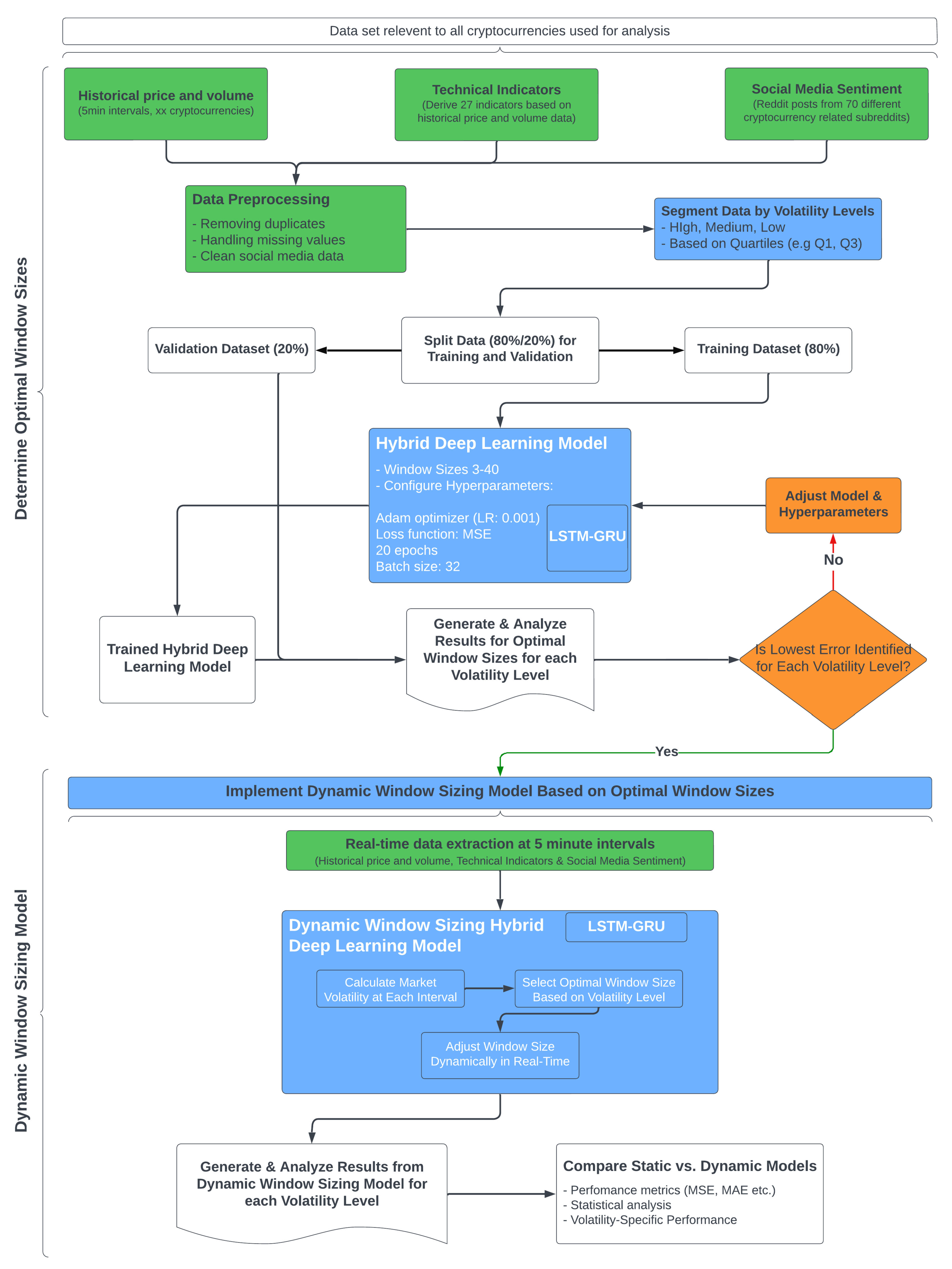
A detailed flowchart is provided in
Figure 1, which visually represents the entire methodological framework, which includes data collection, preprocessing steps, optimal window size identification, dynamic window sizing implementation, and evaluation.
3.3.2. Distinguishing Between Volatility Calculation Window and Prediction Window Size
Before detailing the methods for identifying optimal window sizes, and the implementation of the dynamic window sizing model within the proposed framework, it is essential to highlight the clear distinction between the volatility calculation window and the prediction window size, as each plays a unique and crucial function in the model’s architecture.
Volatility Calculation Window ()
The volatility calculation window, denoted as , is a fixed duration used to assess the underlying market volatility at any given time interval. This window is fixed, and is defined by calculating the standard deviation of cryptocurrency price returns over a specified historical period. The resulting volatility measure helps to classify the current market condition into categories such as high, medium, or low volatility. For example, a 30-day moving standard deviation of daily returns – which is typically used in practice to gauge general market volatility on a macroscopic level – will have a volatility calculation window of 30 time steps (about 1 month).
Prediction Window Size (W)
Contrasting, the prediction window size, denoted as W, is the variable that this study aims to optimise. It defines the period over which the model looks back in time to predict the next price point in the time series, essentially dictating the amount of recent data used for making predictions. The purpose of this paper is to not only optimise the prediction window size but also to dynamically adjust it based on the volatility level identified from the volatility calculation window. For instance, during periods of high volatility, a shorter prediction window may be used to enable the model to quickly adapt to rapid market changes. Conversely, during low volatility periods, a longer prediction window might be preferred to smooth out noise and capture more stable trends. This adaptive approach allows the forecasting model to maintain relevance and accuracy by aligning its input data window with current market dynamics.
Volatility
The volatility at time interval
t, denoted as
, is calculated as the standard deviation of the logarithmic returns over the last
intervals, up to the current time point
t. This is expressed in Equation (
5):
where the logarithmic return
is defined as:
In these equations,
denotes the number of intervals in the
volatility calculation window, and
is the price at the
i-th time interval.
represents the mean of the logarithmic returns over the last
intervals and is given by:
Thus, the volatility measures the dispersion of the logarithmic returns from their mean over the specified window of intervals.
Selecting an appropriate value for
, the volatility calculation window, is crucial as it can significantly impact the results. Traditional approaches typically use daily volatility, aligning with the daily trading cycles of financial markets, particularly stocks, which benefit from the availability of daily closing prices and simplifies the aggregation of volatility measures [
34,
35]. However, the high-frequency nature and unique characteristics of cryptocurrency trading necessitate a departure from these conventions. Cryptocurrency markets operate continuously, 24/7, and generate highly granular data at minute or even second intervals. This high-frequency nature an inherent volatility, requiring a more responsive and nuanced approach to volatility measurement. The dataset utilised in this study, characterised by 5-minute intervals, underscores the need for a volatility calculation window that captures these rapid and frequent fluctuations. Conventional methods prove inadequate for this context, making it imperative to adopt a methodology tailored to the distinctive dynamics of high-frequency cryptocurrency trading.
Hansen and Lunde [
36] underscored the effectiveness of a 30-day rolling window for traditional financial instruments, which aligns with the computation of realised variance from high-frequency intraday returns [
37,
38]. However, this approach does not directly translate to cryptocurrency markets due to their continuous operation, temporal precision and higher volatility. For instance, Guo et al. [
38] demonstrated the utility of using actual historical hourly volatility data, calculated as the standard deviation of minute returns over a one-hour period, highlighting the necessity for shorter, more adaptive windows in high-frequency trading environments.
Given these considerations, this study justifies the selection of a volatility calculation window of 60 intervals (i.e., ), corresponding to 5-minute data points, by the distinct nature of cryptocurrency trading. This 60-interval window, equating to a 5-hour period, provides a balanced approach that captures immediate market movements while maintaining a robust measure of volatility. The rapid fluctuations and dynamic environment of cryptocurrency markets demand a volatility measure that is both timely and sensitive to sudden changes. A 5-hour window is sufficiently short to reflect current market conditions and respond to abrupt price changes, yet long enough to mitigate the noise inherent in high-frequency data – a balance which is critical for developing accurate and reliable forecasting models.
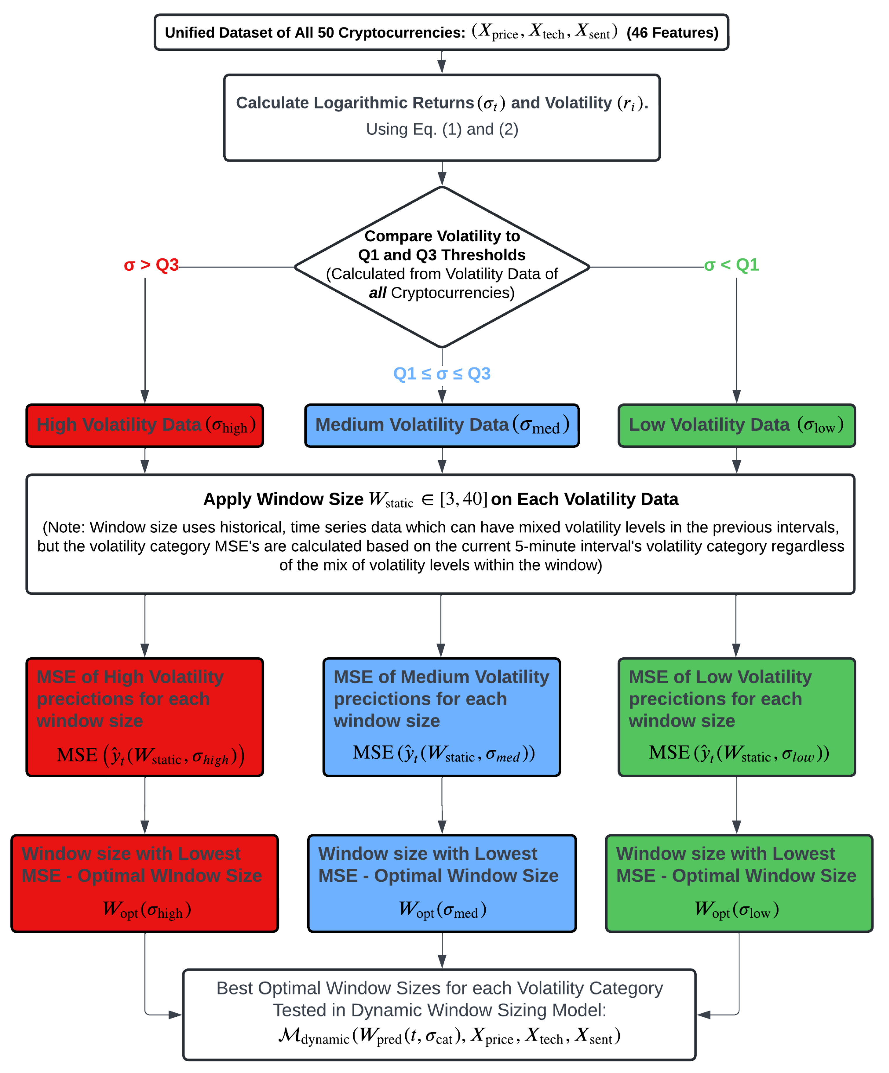
3.3.3. Window Sizing Optimisation Model ()
The following processes outlined in
Section 3.3.3 and
Section 4.2 are summarised visually in
Figure 2, which depicts the segmentation of data based on volatility levels and the corresponding selection of optimal window sizes.
The static deep learning model used for predicting cryptocurrency prices, denoted as
can be described by Equation (
8):
where
is the window size, and
represent the input features: historical price data, technical indicators, and social media sentiment, respectively. This model generates predictions
for future prices. Prior to model training, the logarithmic returns (given by Equation (
6)) are calculated to normalise the data, a standard approach in volatility calculations. The volatility (given by Equation (
5)) is then segmented into three volatility categories ((
)) – high, medium, and low – based on the quarliles of the volatily values for all the data across all cryptocurrencies. This is defined as follows, and is shown quantitatively in Equation (
9):
High Volatility (): Defined by volatility values above the third quartile (Q3), reflecting significant price movements.
Medium Volatility (): Encompassing volatility values between the first quartile (Q1) and the third quartile (Q3), representing moderate market fluctuations.
Low Volatility (): Defined by volatility values below the first quartile (Q1), indicating minimal price fluctuations.
To identify the optimal window size for each volatility category, the model is tested across a range of window sizes
. The optimal window size
for each volatility category
is determined by minimising the mean squared error (MSE) during training and validation, shown in Equation (
10):
where
represents the current volatility category, and
is the window size that minimises MSE for that specific category. These optimal window sizes –
,
, and
– provide valuable insights into the most effective static window sizes for each volatility category. These results serve as the foundation for developing the dynamic window sizing model, in which the prediction window size is dynamically adjusted in real-time based on current market volatility.
3.3.4. Development and Implementation of Dynamic Window Sizing Model ()
The dynamic window sizing model (distinct from the static model ) is specifically designed to adjust the window size in real-time based on current market volatility, ensuring the forecasting model’s responsiveness to fluctuations under various market conditions. This section outlines the quantitative and methodological framework employed to develop, implement, and validate the dynamic window sizing model.
The process begins with the real-time calculation of market volatility at each time interval, categorising it into one of the three predefined levels: high, medium, or low. These levels are determined using thresholds established during the initial optimisation phase, where the rolling standard deviation of logarithmic returns is computed to segment the volatilities – utilising both equations (
5) and (
9).
Based on the identified volatility category, the corresponding prediction window size,
, is dynamically selected. The dynamic window adjustment is formally expressed in Equation (
11):
The core deep learning model of this study, denoted as the
Dynamic Window Sizing Model (
), integrates the dynamically adjusted prediction window
at each time step
t , based on the volatility category
identified from real-time volatility. The dynamic window sizing model can be formally described by Equation (
12):
Unlike the static model, , used to detemine the optimal window sizes, the dynamic model adjusts the window size in real time, enabling it to better align with current market conditions. This dynamic adjustment improves the model’s predictive accuracy by using the appropriate amount of historical data, optimising the balance between short-term responsiveness and long-term trend recognition.
The implementation of the dynamic window sizing model is carried out within the same computational environment described in
Section 3.3.1. The model operates using the same static LSTM-GRU architecture, optimised with the Adam optimiser and Mean Squared Error MSE as the loss function. The real-time dynamic adjustments are managed within a high-performance computing environment, leveraging a GPU-accelerated architecture to handle the computational demands of continuous analysis and dynamic adjustment.
3.4. Comparison with Static Window Models
The dynamic window sizing model’s performance is compared against static models configured with fixed window sizes (3, 4, 5, 6, 7, 8, 9, 10, 12, 15, 20, 25, 30, 35, 40, 45, and 50 periods). These static sizes serve as benchmarks to quantify the improvements offered by dynamic adjustments.
For each window size (), the static models are trained and tested using the same dataset employed to identify the optimal window sizes for the dynamic model. This ensures a direct and fair comparison between the static and dynamic window approaches, with both models operating under identical data conditions.
The static window models, represented by their fixed , serve as baselines to evaluate the dynamic model’s responsiveness to changing market conditions. Specifically, the dynamic model adjusts the window size in real-time, whereas the static models maintain a fixed window size throughout the entire forecasting horizon. Each of these fixed window sizes is tested and compared to the dynamic window sizing model.
The effectiveness of the dynamic model is assessed by comparing its performance across varying volatility levels, focusing on predictive accuracy and the model’s ability to adapt to changing market conditions. The performance improvement achieved by the dynamic window sizing model compared to static models is quantified using the improvement ratio
, formally defined as:
where
refers to the mean squared error of the static model (with
), and
refers to the mean squared error of the dynamic model (with
defined by Equation (
11)) which adjusts the prediction window in real-time based on the identified volatility category
. This metric quantifies the percentage improvement in predictive performance achieved by implementing dynamic window sizing compared to static models, demonstrating how well the dynamic model adapts to varying market conditions and how it compares to models with fixed window sizes. The detailed definition of MSE and other performance metrics used in this analyse will be further expanded upon in the following section.
3.5. Model Evaluation Methodology
For clarity, this section quantitatively defines the evaluation process for predictive models in cryptocurrency price forecasting, with a focus on performance metrics based on the percentage change between consecutive price values. These include quantitative and directional accuracy metrics that are essential for assessing the model’s predictive performance.
3.5.1. Definition of Target Variable
The target variable for model prediction is the percentage change (
y) in cryptocurrency prices, defined for each time interval
i as follows:
where
and
represent the actual prices of the cryptocurrency at time intervals
i and
, respectively.
For clarity in distinguishing between predictions and real market outcomes, the following notation is adopted:
represents the predicted percentage change output by the model for the interval i; while
denotes the actual observed percentage change observed in the market for the same interval, serving as the ground truth for model validation.
3.5.2. Quantitative Performance Metrics
Several metrics are employed to quantitatively evaluate model performance, ensuring a thorough understanding of the forecasts’ accuracy and applicability in real-world scenarios. These metrics are calculated for both training and validation datasets.
Mean Squared Error (MSE)
MSE measures the average of the squared differences between predicted and actual values, emphasising larger errors, which is critical in financial applications for capturing risk.
Root Mean Squared Error (RMSE)
RMSE provides a scale-sensitive measure of error, particularly useful for comparing errors across different datasets or models.
Mean Absolute Error (MAE)
MAE gives a linear measure of the average error magnitude, minimising the influence of outliers and providing a straightforward understanding of error magnitude.
Directional Accuracy Metric ()
Particularly relevant for trading strategies, the directional accuracy,denoted as
, evaluates whether the model correctly predicts the direction of the percentage change, irrespective of its magnitude. This is quantified by Equation (
18):
where
denotes the indicator function, which takes the value 1 when the predicted and actual values share the same sign, and 0 otherwise. This metric evaluates the proportion of correct predictions in terms of the direction of market movements, focusing solely on sign accuracy rather than the magnitude of the change.
These metrics collectively form a overarching evaluation of the model’s predictive performance, ensuring a comprehensive assessment across both the magnitude and direction of market predictions. This allows for a deeper understanding of how well the models adapt to market conditions and how effectively they capture price movements.
4. Results and Discussion
An evaluation of the hybrid LSTM-GRU model was conducted to investigate how varying window sizes influence predictive accuracy in cryptocurrency price forecasting under multiple volatility conditions. The findings provide critical insights into the relationship between volatility and window size, offering both quantitative evidence and theoretical justification that underpin the development of a dynamic window sizing strategy.
4.1. Optimisation of Window Sizes for Volatility Categories
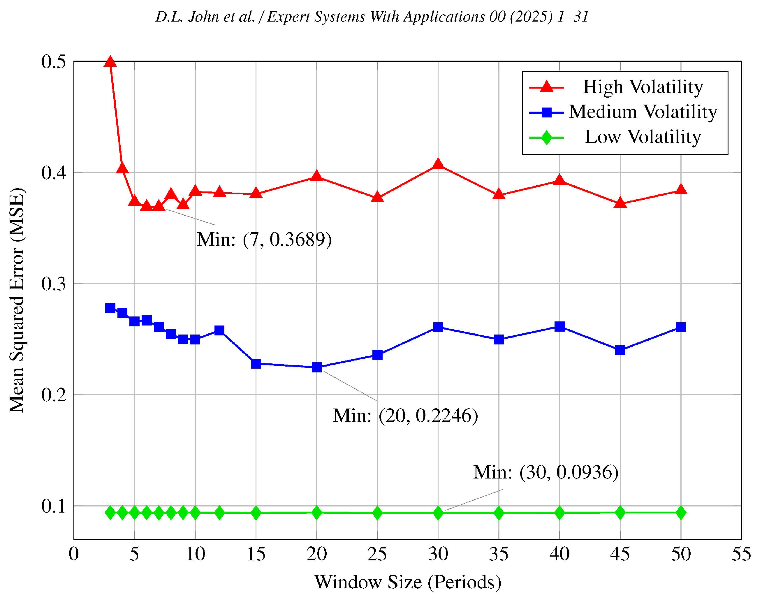
Figure 3 and
Table 4 present the MSE values obtained from the training and validation phases for high, medium, and low volatility data.
4.1.1. High Volatility Conditions
In high volatility conditions, characterised by rapid and significant price fluctuations, the model achieved its lowest validation MSE at a window size of 7, when aggregating results across all cryptocurrency datasets, with an MSE value of 0.3089 as shown in
Table 4. This indicates that, on average, shorter window sizes enhance predictive accuracy in highly volatile markets. Conversely, longer window sizes such as 30 and 40 yield increased MSE values, both in the combined dataset and in individual cryptocurrencies. This pattern is also evident in
Figure 3, where a local minimum is observed at a window size of 7 for the high volatility dataset for the combined data and individual cryptocurrencies.
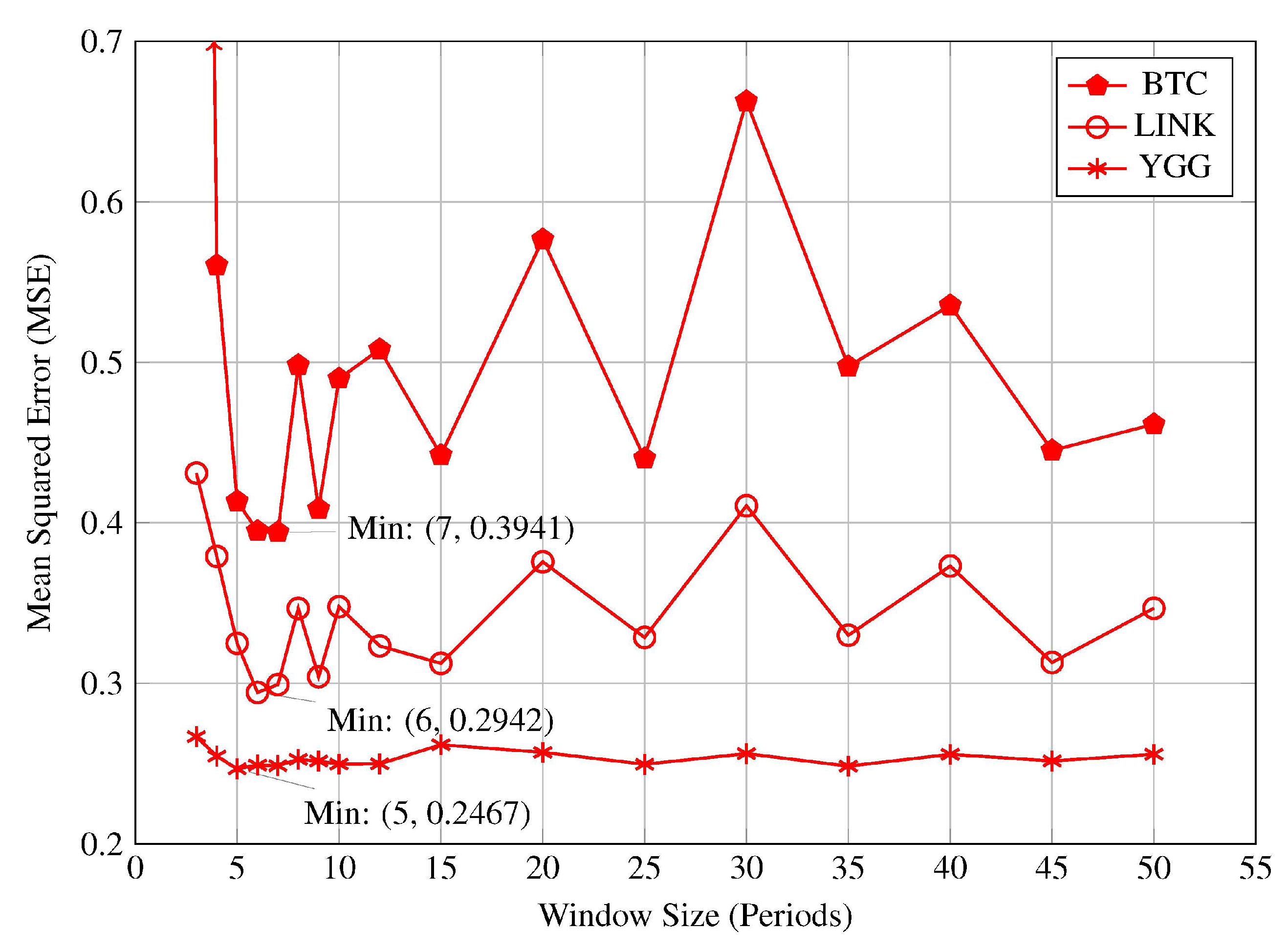
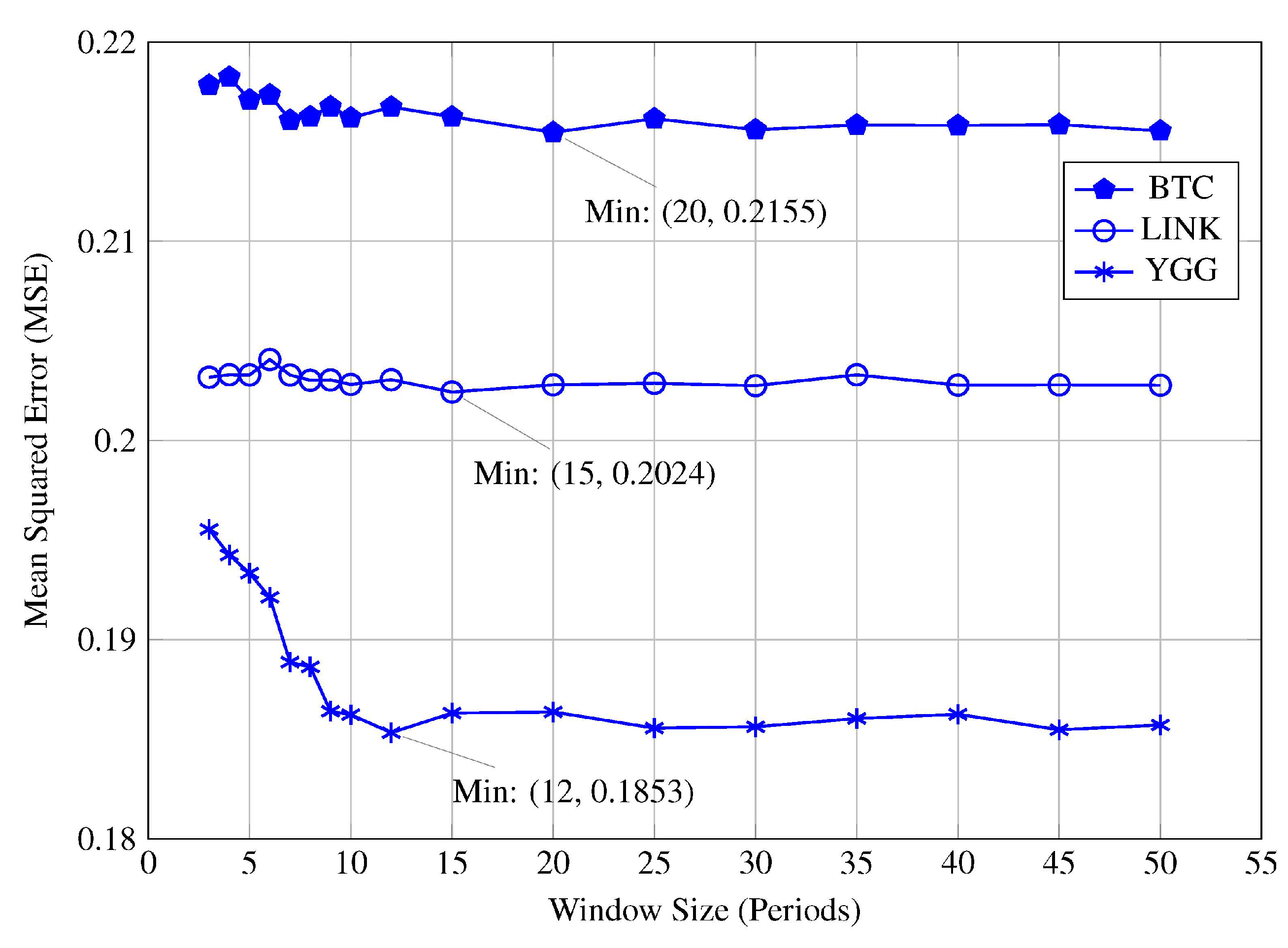
Further analysis of individual cryptocurrency datasets revealed that the model consistently achieved its lowest validation MSE within the window size range of 5 to 7, inclusive. This is illustrated in
Figure 4, which display the MSE profiles for Cryptocurrencies BTC, LINK, and YGG. This consistency across different cryptocurrencies reinforces the conclusion that shorter window sizes are more effective in capturing the rapid market dynamics inherent in high volatility conditions. The superior performance at window sizes 5 to 7 suggests that recent data holds greater relevance for forecasting future price movements when the market is experiencing high volatility. Including older historical data through longer window sizes does not improve, and may even degrade, the model’s performance under these conditions. The increased MSE values associated with longer window sizes imply that older data may introduce noise or outdated information that is not reflective of the current market dynamics. Therefore, in such scenarios, models should prioritise shorter window sizes that focus on recent data to enhance their responsiveness and predictive accuracy.
The observed preference for shorter window sizes in high volatility conditions can be theoretically justified by considering the characteristics of financial time-series data and the underlying market dynamics. In high-volatility markets, prices often shift rapidly due to news events, changing sentiment, or sudden supply–demand imbalances, rendering older data less informative because conditions evolve drastically in short intervals. According to the concept of
volatility clustering or
volatility persistence, periods of high volatility tend to cluster together, meaning that once volatility increases, it often remains elevated for some time [
39,
40,
41]. However, while volatility itself may persist, the direction and patterns of price movements during these periods can be highly unpredictable and erratic.
In such conditions, the most recent data carries more relevant information about the current state of the market. A shorter window size enables the model to concentrate on these recent observations, enhancing its ability to adapt quickly to new market information. This approach aligns with the need for models to be responsive and flexible in volatile environments, where relying on outdated data can hinder predictive accuracy. By focusing on the most current data, the model can better capture sudden market shifts and improve its forecasting performance.
The theoretical justification aligns with the experimental findings, supporting the conclusion that shorter window sizes are more effective in high volatility conditions. The model’s enhanced performance at window sizes 5 to 7 confirms that emphasising recent data is crucial when market conditions are rapidly changing. This understanding is critical for developing forecasting models that can adapt to high volatility environments, such as cryptocurrency markets, where price dynamics can be highly unpredictable.
4.1.2. Medium Volatility Conditions
In medium volatility conditions, characterised by moderate but consistent price fluctuations, the model achieved its lowest validation MSE at a window size of 20, with an MSE value of 0.2261, as shown in
Table 4. In contrast, both shorter window sizes (e.g., 3 to 7) and longer window sizes (e.g., 40 to 50) yielded higher MSE values.
Figure 3 also illustrates this pattern, revealing a local minimum at a window size of 20, which aligns with the optimal model performance under medium volatility conditions.
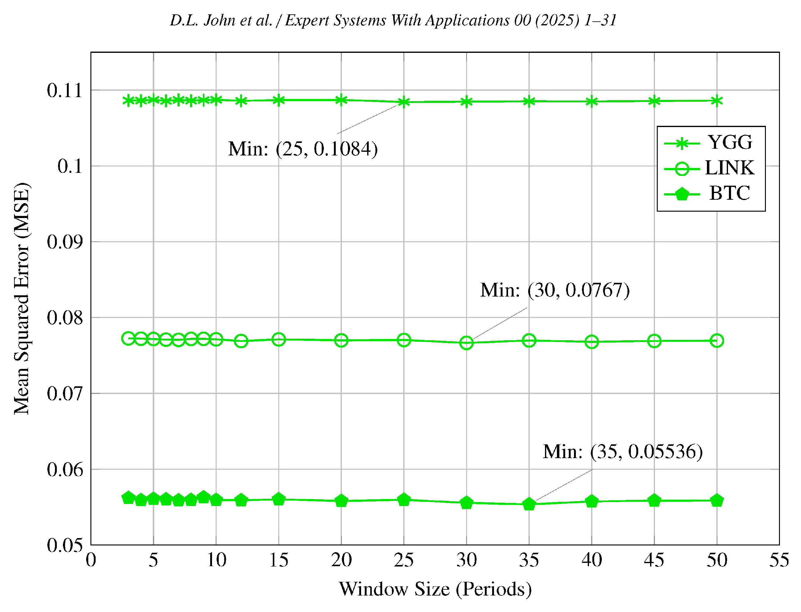
Moreover, analysis of individual cryptocurrency datasets revealed that the model consistently achieved its lowest validation MSE within the window size range of 12 to 20, inclusive, as illustrated in
Figure 5. This consistency across different cryptocurrencies suggests that intermediate window sizes strike an effective balance between recent and historical data, accommodating the moderate fluctuations characteristic of medium volatility markets. The comparatively higher MSE values at both shorter and longer windows imply that overly short windows may exclude useful older information, whereas longer windows can introduce outdated data, reinforcing the need for a moderate window length to capture gradual yet significant changes.
This observed preference can be theoretically justified by the nature of price movements in such markets. Medium volatility markets exhibit price fluctuations that are less extreme than those seen in high volatility settings but are more dynamic than low volatility conditions. This characteristic indicates that while recent data is important for capturing current trends, slightly older data also contributes valuable context that aids in identifying gradual shifts. The principle of mean reversion, which is more pronounced in medium and low volatility settings, suggests that asset prices often tend to revert towards a longer-term trend (i.e., their historical average), following short-term deviations [
42,
43,
44]. In medium volatility conditions, this mean-reverting tendency means that incorporating an appropriate range of historical data allows the model to recognise these cyclical adjustments and respond accordingly. By including both recent and somewhat older data through an intermediate window size, the model benefits from a more comprehensive view of ongoing market conditions, enhancing its ability to track gradual changes and forecast future movements more accurately.
The theoretical justification aligns with the quantitative findings, confirming that intermediate window sizes are most suitable in medium volatility conditions. The model’s improved performance at moderate window sizes suggests that medium volatility conditions benefit from a balanced approach, where the model leverages both recent data and slightly older trends. This understanding is essential for refining forecasting models in medium volatility environments, where market conditions are moderately volatile and require a nuanced balance between short-term responsiveness and long-term trend awareness.
4.1.3. Low Volatility Conditions
In contrast, the analysis under low volatility conditions, marked by gradual and stable price movements, demonstrates consistently low and stable MSE values across a range of window sizes. The minimum MSE occurs at a window size of 30, with values spanning narrowly between 0.0936 and 0.0941, as displayed in
Table 4.
Figure 3 illustrates the near-constant MSE across different window sizes, indicates that the model generalises effectively across different window sizes when volatility is minimal.
Analysis of individual cryptocurrencies under low volatility conditions supports this observation.
Figure 6 show that MSE values remain consistently low across all window sizes even for individual Cryptocurrencies such as AMP, AUROA, and SHIB. The model’s uniform accuracy across all window sizes suggests that the volume of historical data included has a negligible impact on forecasting accuracy. This consistency implies that in low volatility environments, where trends are steady and significant price shifts are uncommon, both recent and extended historical data are similarly effective. The negligible differences in MSE highlight that the model more effectively captures patterns in these environments, making the choice of window size less critical.
Theoretical justification for this stability lies in the steady nature of price movements in low volatility markets. In such settings, prices follow long-term trends influenced primarily by fundamental factors rather than sudden, unpredictable shifts. The concept of mean reversion is less pronounced compared to medium volatility conditions, as price deviations from the mean occur less frequently and with smaller magnitudes. Consequently, the choice of window size has limited impact, enabling reliable and consistent forecasting in these environments. This reinforces the model’s capacity to maintain high accuracy and adaptability under stable market conditions.
4.1.4. Impact of Window Size on Predictive Accuracy Across Volatility Levels
The analysis of MSE across varying market volatility levels reveals a consistent pattern: MSE values escalate progressively from low to high volatility, persisting across all tested window sizes. This trend, visually depicted in
Figure 3 and supported by empirical data in
Table 4, underscores the intrinsic relationship between market stability and forecasting accuracy. Specifically, increased price fluctuations are directly proportional to forecasting errors in predictive analyses.
The notably lower MSE observed in low volatility settings can primarily be attributed to the market’s minimal fluctuations. In these environments, the market exhibits stable and predictable patterns, allowing the model to capture underlying trends more accurately. Consequently, the smaller percentage changes in predictions – when incorrect – result in inherently minor errors due to the consistently low variability in the data. This characteristic renders the choice of window size less critical in low volatility conditions.
Conversely, medium volatility data display intermediate MSE values, reflecting the model’s capability to capture trends with reasonable accuracy. However, the increased variability introduces greater forecasting errors compared to low volatility scenarios. Similarly, high volatility data consistently exhibit the highest and most variable MSE values due to the larger percentage changes in price. In these conditions, incorrect predictions result in significantly larger errors, challenging the model’s predictive capabilities and resulting in greater discrepancies between forecasted and actual values. This variability underscores the model’s sensitivity to window size selection in higher volatility settings, highlighting the necessity for optimal window size configurations to improve predictive accuracy.
The empirical justification for these observations lies in the mathematical properties of the MSE calculation. MSE is defined as the average of the squares of the errors between predicted and actual values. In low volatility conditions, the errors between the model’s predictions and the actual values are consistently small due to the stable nature of the data, resulting in lower MSE values. Conversely, as volatility increases, the substantial fluctuations and inherent unpredictability of the market lead to larger prediction errors, thereby increasing the MSE. This pattern demonstrates the critical role of volatility in influencing predictive accuracy and underscores the importance of selecting optimal window sizes to manage the higher predictive uncertainty in medium and high volatility environments.
4.2. Optimal Window Sizes Across Volatility Categories
Based on the findings, distinct ranges of optimal window sizes were identified for each volatility category across the cryptocurrencies analysed. In
high volatility conditions, the MSE profiles exhibited minimum at a window sizes ranging 5 to 7 across all cryptocurrencies, with MSE values increasing for larger window sizes (see
Figure 3 and
Figure 4 and
Table 4). These minima at shorter window lengths indicate that shorter window sizes are optimal in highly volatile markets, as they captures the most recent and relevant fluctuations without the noise introduced by older, less pertinent data.
In
medium volatility conditions, the MSE profile showed pronounced minima at window sizes ranging from 12 to 20 (see
Figure 3 and
Figure 5 and
Table 4). Window sizes shorter than 12 failed to encompass essential historical trends necessary for accurate predictions, while longer window sizes began to incorporate outdated information that did not contribute to predictive accuracy. This suggests that intermediate window sizes are most effective in capturing the relevant market trends and enhancing predictive accuracy in medium volatility environments.
For
low volatility conditions, the MSE values remained relatively constant across all tested window sizes, indicating that the model’s predictive accuracy was less sensitive to the amount of historical data included (see
Figure 3 and
Figure 6 and
Table 4). However, a subtle minimum in MSE was noted at window sizes ranging from 25 to 35 periods, suggesting that including more historical data may be slightly beneficial. This implies that in stable markets, where trends are gradual and consistent, longer window sizes can be advantageous by capturing long-term patterns without the detriment of excessive noise. Consequently, larger window sizes ensure comprehensive inclusion of relevant historical data, thereby marginally enhancing predictive performance in low volatility environments.
4.2.1. Development and Configuration of the Dynamic Window Sizing Model
Building upon the identification of optimal window sizes for different volatility categories, the dynamic window sizing model, denoted as , was developed. The primary objective of is to adaptively adjust the prediction window based on real-time market volatility, thereby enhancing predictive accuracy across varying market conditions.
To construct , the previously identified optimal window sizes for high, medium, and low volatility categories were utilised: , , and . All of the combinations of these optimal window sizes – yielding a total of 27 configurations (3 × 3 × 3) – were systematically tested together across the dataset comprising 50 cryptocurrencies, to determine the most effective overall model configuration.
The performance of each configuration was assessed using key evaluation metrics: MSE, RMSE, MAE, and Directional Accuracy (
). The aggregation of these performance metrics are presented in
Table 5, which facilitated the identification of the overall optimal configuration.
that consistently yielded the lowest error rates and highest directional accuracy.
As shown in
Table 5, the dynamic model configuration yielding the lowest validation MSE and highest corresponds to the following optimal window sizes for each volatility category:
High Volatility: Optimal window size
Medium Volatility: Optimal window size
Low Volatility: Optimal window size
This optimal configuration represents the most effective combination of window sizes tailored to high, medium, and low volatility conditions, which serve as the foundation for the dynamic window sizing model. By adopting these optimal window sizes, this enables the model to dynamically select the appropriate window size () based on the current market volatility . This adaptive approach ensures that the prediction window is precisely aligned with prevailing market conditions, thereby enhancing predictive accuracy.
4.3. Performance Evaluation of the Dynamic Model
Following the development and configuration of the dynamic window sizing model
as detailed in
Section 4.2.1, its predictive performance was rigorously evaluated against all static models with fixed window sizes ranging from 3 to 50 periods. This evaluation aimed to ascertain the efficacy of the dynamic model in enhancing predictive accuracy across varying market volatility conditions.
Table 6 presents the performance metrics of the dynamic model
in comparison to static models with fixed window sizes. Additionally,
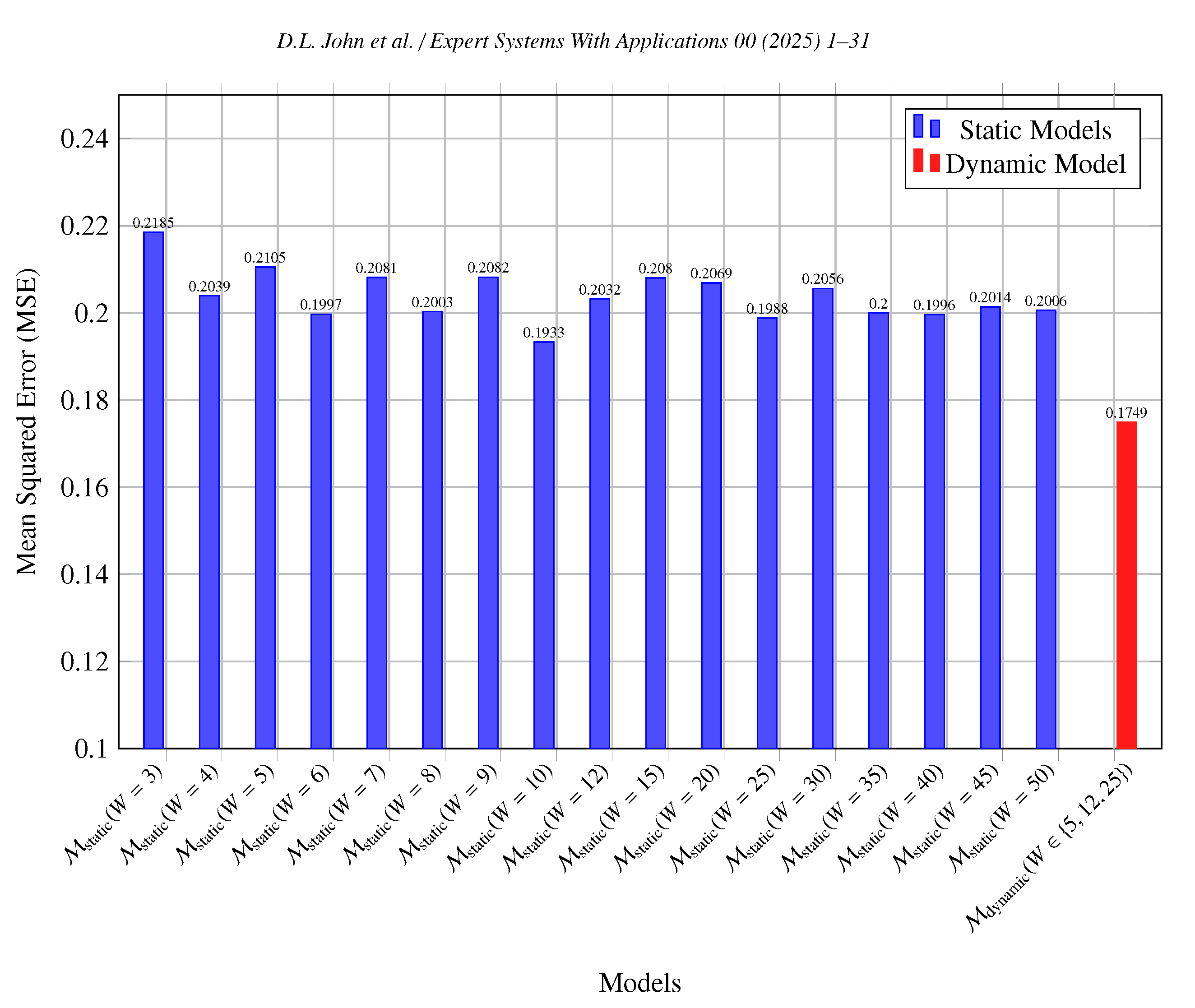
Figure 7 visualises the MSE values of static models across different window sizes alongside the dynamic model.
The comparative analysis, as illustrated in
Table 6 and
Figure 7, demonstrates that the dynamic window sizing model consistently outperforms all static models across all evaluated metrics. Specifically,
achieved the lowest MSE and MAE values of 0.1749 and 0.2281 respectively, coupled with the highest directional accuracy (
) of 56.77%, underscoring its superior predictive capabilities (see
Table 6). In contrast, the best-performing static model, with a window size of 10 periods, recorded an MSE of 0.1933, an MAE of 0.2883 and a directional accuracy (
) of 49.11%, but still underperformed relative to the dynamic model. This indicates that
not only reduces predictive errors but also enhances the model’s ability to accurately forecast price movements. The dynamic model’s superior performance can be visually seen in
Figure 7, which highlights its high predictive accuracy, adaptability and effectiveness in managing different market conditions. This visualisation complements the quantitative results presented in
Table 6, offering a clear and intuitive understanding of the advantages dynamic model’s have over static configurations.
Furthermore, demonstrated consistent performance across various cryptocurrency assets, highlighting its generalisability and robustness in diverse market conditions. The elevated directional accuracy () further emphasises the model’s proficiency in correctly predicting the direction of price movements, which is critical for strategic trading decisions.
This performance evaluation demonstrates that the dynamic window sizing model surpasses static models in predictive accuracy at varying volatility levels. By dynamically adjusting the prediction window based on real-time market volatility, effectively mitigates the limitations of static window sizing, providing a more reliable and accurate forecasting mechanism in the volatile cryptocurrency market.
5. Future Work
Although the dynamic window sizing methodology has demonstrated substantial improvements in cryptocurrency price forecasting, several opportunities exist for further enhancement and broader applicability. Extending the proposed framework to domains beyond cryptocurrency markets, such as high-frequency trading in equity markets, energy load prediction, or real-time network traffic analysis, may validate its generalisability. In these contexts, verifying the method’s adaptability and robustness would provide stronger evidence of its practical value and adaptability.
Refining the categorisation of volatility beyond the three broad classes employed in this study also warrants attention. Introducing more granular segmentation schemes may enable the model to adjust window sizes with greater precision, thus improving its capacity to track complex market scenarios. This refinement could be complemented by integrating reinforcement learning or other adaptive optimisation techniques, allowing the model to learn optimal strategies continuously from streaming data rather than relying on predefined thresholds. Such enhancements would promote long-term scalability and resilience, ensuring that the model remains effective even as underlying conditions evolve.
Additionally, investigating more advanced architectures and incorporating additional data sources offers another promising avenue. While this work integrates technical indicators and social media sentiment, introducing alternative data streams – such as blockchain transaction activity or macroeconomic indicators – may reveal latent patterns not captured by more conventional signals. Complementary architectural innovations, including Transformers, Temporal Convolutional Networks, or hybrid models that combine deep learning with probabilistic methods, could further improve the model’s ability to represent intricate temporal dependencies. Employing attention mechanisms within these architectures may enable selective focus on critical input segments, thereby enhancing interpretability and accuracy under dynamic market conditions.
Finally, addressing practical deployment constraints remains critical for real-time applications. Ensuring computational efficiency, accommodating low-latency requirements, and adopting parallelisation strategies will facilitate real-time execution at scale. Balancing accuracy and speed is of high importance, as delays or inefficiencies may hinder decision-making processes in live environments. By addressing these areas, future work can foster the development of more robust, versatile, and practically deployable models, ultimately extending the benefits of dynamic window sizing across a broader spectrum of time-series forecasting applications.
6. Conclusions
This research demonstrates that dynamically optimising window sizes based on market volatility significantly improves time-series forecasting performance, specifically within the cryptocurrency domain. By establishing that shorter historical windows enhance accuracy under high volatility, intermediate windows excel in medium volatility conditions, and longer windows marginally benefit low volatility scenarios, the study provides a clear framework for tailoring window sizes to prevailing market conditions.
The introduction of a hybrid LSTM-GRU model integrated with dynamic window sizing underscores the advantages of real-time adaptability. Compared to static window configurations, the dynamic approach consistently produces lower forecasting errors and higher directional accuracy. These outcomes confirm that incorporating volatility-driven window size selection better aligns the model’s training perspective with underlying market conditions, thus improving predictive reliability and interpretability.
This research provides valuable insights that extend beyond cryptocurrency markets, potentially informing a broad array of time-series forecasting tasks where adaptability and responsiveness are essential. By demonstrating how dynamically optimised window sizes can better align model inputs with rapidly changing data patterns, this work highlights the importance of refining how historical information is integrated into forecasting models. These findings set the stage for future advancements, including more granular approaches to volatility segmentation, the incorporation of additional data sources, and the exploration of alternative deep learning architectures. Taken together, these potential directions contribute to the development of more flexible and robust predictive models, capable of effectively navigating the evolving complexities of digital-era data streams.
References
- Wang, Z.; Chen, Y.; Hu, W. Deep Learning Models for Time Series Forecasting: A Review. IEEE Access 2021, 9, 123456–123469. [Google Scholar]
- Lara-Benítez, P.; Carranza-García, M.; Riquelme, J.C. Deep Learning-Based Time Series Forecasting: A Review. Artificial Intelligence Review 2021, 54, 537–574. [Google Scholar]
- Tao, Z.; Xu, Q.; Liu, X.; Liu, J. An Integrated Approach Implementing Sliding Window and DTW Distance for Time Series Forecasting Tasks. Applied Intelligence 2023, 53, 20614–20625. [Google Scholar] [CrossRef]
- Torres, A.; Ortega, J.A.; Díez, J.F. Deep Learning for Time Series Forecasting: Advances and Open Challenges. Information 2023, 14, 598. [Google Scholar]
- Tanwar, S.; Patel, N.P.; Patel, S.N.; Patel, J.R.; Sharma, G.; Davidson, I.E. Deep learning-based cryptocurrency price prediction scheme with inter-dependent relations. IEEE Access 2021, 9, 138633–138646. [Google Scholar] [CrossRef]
- Albariqi, R.; Winarko, E. Prediction of bitcoin price change using neural networks. In Proceedings of the 2020 international conference on smart technology and applications (ICoSTA). IEEE, 2020, pp. 1–4.
- Chiong, R.; Fan, Z.; Hu, Z.; Dhakal, S. A Novel Ensemble Learning Approach for Stock Market Prediction Based on Sentiment Analysis and the Sliding Window Method. IEEE Transactions on Computational Social Systems 2023, 10, 2613–2623. [Google Scholar] [CrossRef]
- Kumar, M.R.; Umar, S.; Venkatram, V. Short Term Memory Recurrent Neural Network-based Machine Learning Model for Predicting Bit-coin Market Prices. In Proceedings of the 14th International Conference on Advances in Computing, Control, and Telecommunication Technologies, ACT 2023, 2023, Vol. 2023-June, pp. 1683–1689.
- Kelotra, A.; Pandey, P. Stock market prediction using optimized deep-convlstm model. Big Data 2020, 8, 5–24. [Google Scholar] [CrossRef] [PubMed]
- Kilimci, H.; Yıldırım, M.; Kilimci, Z.H. The Prediction of Short-Term Bitcoin Dollar Rate (BTC/USDT) using Deep and Hybrid Deep Learning Techniques. In Proceedings of the 2021 5th International Symposium on Multidisciplinary Studies and Innovative Technologies (ISMSIT), 2021, pp. 633–637. [CrossRef]
- Azlan, A.; Yusof, Y.; Mohsin, M.F.M. Determining the Impact of Window Length on Time Series Forecasting Using Deep Learning. International Journal of Advanced Computer Research 2019, 9, 260–267. [Google Scholar] [CrossRef]
- Freitas, J.; Ponte, C.; Bomfim, R.; Caminha, C. The impact of window size on univariate time series forecasting using machine learning. In Proceedings of the Anais do XI Symposium on Knowledge Discovery, Mining and Learning, Porto Alegre, RS, Brasil, 2023; pp. 65–72. [Google Scholar] [CrossRef]
- Wen, N.S.; Ling, L.S. Evaluation of Cryptocurrency Price Prediction Using LSTM and CNNs Models. International Journal on Informatics Visualization 2023, 7, 2016–2024. [Google Scholar] [CrossRef]
- Lei, K.; Zhang, B.; Li, Y.; Yang, M.; Shen, Y. Time-driven feature-aware jointly deep reinforcement learning for financial signal representation and algorithmic trading. Expert Systems with Applications 2020, 140, 112872. [Google Scholar] [CrossRef]
- Rajabi, S.; Roozkhosh, P.; Farimani, N.M. MLP-based Learnable Window Size for Bitcoin price prediction. Applied Soft Computing 2022, 129, 109584. [Google Scholar] [CrossRef]
- Ingale, O. Exploration of Stacked Ensemble Models for Bitcoin Price Prediction Using Diverse Look-Back Windows, 2023. [CrossRef]
- Shynkevich, Y.; McGinnity, T.; Coleman, S.A.; Belatreche, A.; Li, Y. Forecasting price movements using technical indicators: Investigating the impact of varying input window length. Neurocomputing 2017, 264, 71–88, Machine learning in finance. [Google Scholar] [CrossRef]
- Andrade de Oliveira, F.; Enrique Zárate, L.; de Azevedo Reis, M.; Neri Nobre, C. The use of artificial neural networks in the analysis and prediction of stock prices. In Proceedings of the 2011 IEEE International Conference on Systems, Man, and Cybernetics, 2011, pp. 2151–2155. [CrossRef]
- TechCrunch. Twitter to end free access to its API 2023.
- Company, F. Elon Musk’s Twitter API Changes: Monetization and the Impact on Users 2023.
- AOL. Elon Musk backtracks on Twitter API decision after developer backlash, 2023.
- Press, T. Comparing Platform Research API Requirements, 2023.
- Blog, R. 13 Top Social Media APIs & Free Alternatives List - April, 2024, 2024.
- Roach, J. Why everyone is freaking out about the Reddit API right now. Digital Trends 2023.
- Help, R. Reddit Data API Wiki, 2024. Accessed: 2024-05-01.
- Reddit. Creating a Healthy Ecosystem for Reddit Data and Reddit Data API Access, 2023. Accessed: 2024-05-01.
- Reddit Data API Wiki. https://support.reddithelp.com/hc/en-us/articles/360043034832-Reddit-Data-API-Wiki, 2024.
- John, D.L.; Stantic, B. Machine Learning or Lexicon Based Sentiment Analysis Techniques on Social Media Posts. In Proceedings of the Asian Conference on Intelligent Information and Database Systems; Nguyen, N.T.; Tran, T.K.; Tukayev, U.; Hong, T.P.; Trawiński, B.; Szczerbicki, E., Eds. Springer, Springer Nature Switzerland, 2022, pp. 3–12.
- Hutto, C.; Gilbert, E. Vader: A parsimonious rule-based model for sentiment analysis of social media text. In Proceedings of the Proceedings of the International AAAI Conference on Web and Social Media, 2014, Vol. 8.
- Stantic, B.; Mandal, R.; Chen, E. Target Sentiment and Target Analysis. Report to the National Environmental Science Program. Reef and Rainforest Research Centre Limited, Cairns 2020.
- Kathuria, P. Sentiment classification using WSD, maximum entropy and Naive Bayes classifiers, 2014.
- Alaei, A.R.; Becken, S.; Stantic, B. Sentiment analysis in tourism: Capitalizing on big data. Journal of Travel Research 2019, 58, 175–191. [Google Scholar] [CrossRef]
- Ter-Avanesov, B.; Beigi, H. MLP, XGBoost, KAN, TDNN, and LSTM-GRU Hybrid RNN with Attention for SPX and NDX European Call Option Pricing. arXiv, 2024; arXiv:2409.06724. [Google Scholar]
- Bollen, B.; Inder, B. Estimating daily volatility in financial markets utilizing intraday data. Journal of Empirical Finance, 9, 551–562. [CrossRef]
- Fleming, J.; Ostdiek, B.; Whaley, R.E. Predicting stock market volatility: A new measure. The Journal of Futures Markets (1986-1998) 1995, 15, 265. [Google Scholar] [CrossRef]
- Hansen, P.R.; Lunde, A. A forecast comparison of volatility models: Does anything beat a GARCH (1, 1)? Journal of applied econometrics 2005, 20, 873–889. [Google Scholar] [CrossRef]
- Malladi, R.K.; Dheeriya, P.L. Time series analysis of cryptocurrency returns and volatilities. Journal of Economics and Finance 2021, 45, 75–94. [Google Scholar] [CrossRef]
- Guo, T.; Antulov-Fantulin, N. Predicting short-term Bitcoin price fluctuations from buy and sell orders. arXiv, 2018; arXiv:1802.04065. [Google Scholar]
- Gang-Jin Wang, Chi Xie, K.H.; Stanley, H.E. Extreme risk spillover network: Application to financial institutions. Quantitative Finance 2017, 17, 1417–1433. [CrossRef]
- Cont, R. Empirical properties of asset returns: Stylized facts and statistical issues. Quantitative Finance 2001, 1, 223–236. [Google Scholar] [CrossRef]
- Mandelbrot, B.B.; Mandelbrot, B.B. The variation of certain speculative prices; Springer, 1997.
- Poterba, J.M.; Summers, L.H. Mean reversion in stock prices: Evidence and Implications. Journal of Financial Economics 1988, 22, 27–59. [Google Scholar] [CrossRef]
- Lo, A.W.; MacKinlay, A.C. Stock market prices do not follow random walks: Evidence from a simple specification test. The review of financial studies 1988, 1, 41–66. [Google Scholar] [CrossRef]
- Chinthapalli, U.R. A Comparative Analysis on Probability of Volatility Clusters on Cryptocurrencies, and FOREX Currencies. Journal of Risk and Financial Management 2021, 14. [Google Scholar] [CrossRef]
Figure 1.
Flowchart illustrating the methodological framework for dynamic window sizing in cryptocurrency price forecasting, including data collection, preprocessing, optimal window size identification, dynamic adjustment, and evaluation
Figure 1.
Flowchart illustrating the methodological framework for dynamic window sizing in cryptocurrency price forecasting, including data collection, preprocessing, optimal window size identification, dynamic adjustment, and evaluation
Figure 2.
Flowchart depicting the process of data segmentation based on volatility categories and the selection of optimal window sizes through MSE minimisation.
Figure 2.
Flowchart depicting the process of data segmentation based on volatility categories and the selection of optimal window sizes through MSE minimisation.
Figure 3.
Comparison of validation MSE across different window sizes and volatility categories (high, medium, and low), showing how optimal window sizes vary for each condition.
Figure 3.
Comparison of validation MSE across different window sizes and volatility categories (high, medium, and low), showing how optimal window sizes vary for each condition.
Figure 4.
Comparison of MSE across different window sizes for three cryptocurrencies (BTC, LINK, and YGG) under high volatility conditions, highlighting the optimal window sizes for each asset.
Figure 4.
Comparison of MSE across different window sizes for three cryptocurrencies (BTC, LINK, and YGG) under high volatility conditions, highlighting the optimal window sizes for each asset.
Figure 5.
Comparison of MSE across different window sizes for three cryptocurrencies (BTC, LINK, and YGG) under medium volatility conditions, highlighting the optimal window sizes for each asset.
Figure 5.
Comparison of MSE across different window sizes for three cryptocurrencies (BTC, LINK, and YGG) under medium volatility conditions, highlighting the optimal window sizes for each asset.
Figure 6.
Comparison of MSE across different window sizes for three cryptocurrencies (BTC, LINK, and YGG) under low volatility conditions, highlighting the optimal window sizes for each asset.
Figure 6.
Comparison of MSE across different window sizes for three cryptocurrencies (BTC, LINK, and YGG) under low volatility conditions, highlighting the optimal window sizes for each asset.
Figure 7.
Comparison of MSE between static models with fixed window sizes, ranging from 3 to 50 periods, and the dynamic window sizing model. The dynamic model achieves a lower MSE than all static configurations, indicating superior predictive performance.
Figure 7.
Comparison of MSE between static models with fixed window sizes, ranging from 3 to 50 periods, and the dynamic window sizing model. The dynamic model achieves a lower MSE than all static configurations, indicating superior predictive performance.
Table 1.
List of technical indicators used, including their mathematical formulations and definitions.
Table 1.
List of technical indicators used, including their mathematical formulations and definitions.
| Technical Indicator |
Equation |
Definition |
| Simple Moving Avg. (SMA) |
|
Average closing price over a the last n periods. |
| Exponential Moving Avg. (EMA) |
|
Weighted average that gives more importance to recent prices. |
| Relative Strength Index (RSI) |
|
Measures price momentum to identify overbought or oversold conditions. |
| Moving Avg. Con/Div (MACD) |
|
Shows relationship between two EMA’s for buy and sell signals. |
| MACD Signal Line (MACDSig) |
|
Represents the exponential weighted moving average of the MACD, used to trigger buy or sell signals. |
| Standard Deviation (STDn) |
|
Calculates the standard deviation of the last price over the last n periods. |
| Upper Bollinger Band (BBU) |
|
Acts as a resistance level, typically indicating overbought conditions. |
| Lower Bollinger Bands (BBL) |
|
Acts as a support level, typically suggesting oversold conditions. |
| Moving Average Envelope (MAEn) |
|
A channel around the SMA of width , identifying overbought (Upper Envelope, UE) and oversold levels (Lower Envelope, LE). |
| Momentum (MOM) |
|
Measures the change in price indicating the strength of the trend. |
| Force Index (FI) |
|
Measures the strength of buying and selling pressure, indicating potential trend reversals. |
| Average Gain/Loss (AG, AL) |
|
Calculates average gain and loss in price (separately) over a specific number of periods. |
| Triangular Moving Average (TMA) |
|
A weighted moving average that is more responsive to recent price changes. |
| McGinley Dynamic Indicator (MDI) |
|
A dynamical adaptive moving average, reducing lag and providing smoother trends. |
| Price Volume Trend (PVT) |
|
Measures the relationship between price and volume, indicating the strength of price trends. |
| Volume Weighted Mov. Avg. (VWMA) |
|
Calculates average price weighted by trading volume to assess average entry price. |
| Trend Strength (TS) |
|
Indicates the strength of a trend by comparing short and long-term moving averages relative to the last price. |
| Up/Down Trend Indicator (UDTI) |
|
Assigns a trend direction based on the trend strength; positive for upward, negative for downward, and neutral for no trend. |
| Logarithmic Returns () |
|
Calculates the logarithm of the ratio of the current price to the previous price, indicating the continuous rate of return. |
| Volatility (VOL60) |
|
Calculates the standard deviation of the logarithmic returns over the last 60 periods, indicating market volatility. |
| Percent Change (PC) |
|
Measures the percentage change in price from the previous period to the current period. |
Table 2.
Example of preprocessed input data sequence for high volatility periods using a window size of 3, zero-padded to maintain consistent input dimensions.
Table 2.
Example of preprocessed input data sequence for high volatility periods using a window size of 3, zero-padded to maintain consistent input dimensions.
| Time Step |
Feature 1 |
Feature 2 |
⋯ |
Feature 46 |
| Padding 1 |
0 |
0 |
⋯ |
0 |
| Padding 2 |
0 |
0 |
⋯ |
0 |
| Padding 3 |
0 |
0 |
⋯ |
0 |
| Padding 4 |
0 |
0 |
⋯ |
0 |
|
|
|
⋯ |
|
|
|
|
⋯ |
|
| t |
|
|
⋯ |
|
Table 3.
Example of input data sequence for low volatility periods using a window size of 7, illustrating the use of full data without zero-padding.
Table 3.
Example of input data sequence for low volatility periods using a window size of 7, illustrating the use of full data without zero-padding.
| Time Step |
Feature 1 |
Feature 2 |
⋯ |
Feature 46 |
|
|
|
⋯ |
|
|
|
|
⋯ |
|
|
|
|
⋯ |
|
|
|
|
⋯ |
|
|
|
|
⋯ |
|
|
|
|
⋯ |
|
| t |
|
|
⋯ |
|
Table 4.
MSE values for training and validation data across different window sizes and volatility categories (high, medium, and low).
Table 4.
MSE values for training and validation data across different window sizes and volatility categories (high, medium, and low).
| Window |
High Volatility |
Medium Volatility |
Low Volatility |
| Size |
Training |
Val. |
Training |
Val. |
Training |
Val. |
| 3 |
0.4362 |
0.4984 |
0.2639 |
0.2681 |
0.0867 |
0.0941 |
| 4 |
0.3369 |
0.4027 |
0.2589 |
0.2634 |
0.0864 |
0.0940 |
| 5 |
0.3318 |
0.3733 |
0.2507 |
0.2559 |
0.0858 |
0.0940 |
| 6 |
0.3358 |
0.3691 |
0.2502 |
0.2569 |
0.0861 |
0.0940 |
| 7 |
0.3441 |
0.3689 |
0.2441 |
0.2509 |
0.0872 |
0.0938 |
| 8 |
0.3394 |
0.3797 |
0.2366 |
0.2445 |
0.0874 |
0.0939 |
| 9 |
0.3399 |
0.3704 |
0.2315 |
0.2398 |
0.0874 |
0.0941 |
| 10 |
0.3424 |
0.3824 |
0.2314 |
0.2398 |
0.0863 |
0.0939 |
| 12 |
0.3439 |
0.3814 |
0.2161 |
0.2328 |
0.0866 |
0.0939 |
| 15 |
0.34369 |
0.3805 |
0.2163 |
0.2281 |
0.0862 |
0.0938 |
| 20 |
0.3372 |
0.3958 |
0.2217 |
0.2246 |
0.0865 |
0.0940 |
| 25 |
0.3468 |
0.3768 |
0.2196 |
0.2357 |
0.0867 |
0.0937 |
| 30 |
0.3395 |
0.4065 |
0.2306 |
0.2457 |
0.0861 |
0.0936 |
| 35 |
0.3438 |
0.3793 |
0.2194 |
0.2347 |
0.0862 |
0.0939 |
| 40 |
0.3433 |
0.3923 |
0.2379 |
0.2514 |
0.0863 |
0.0938 |
| 45 |
0.3401 |
0.3716 |
0.2199 |
0.2301 |
0.0862 |
0.0939 |
| 50 |
0.3378 |
0.3835 |
0.2426 |
0.2507 |
0.0865 |
0.0940 |
Table 5.
Performance metrics for various combinations of optimal window sizes across volatility categories, used to determine the best configuration for the dynamic window sizing model.
Table 5.
Performance metrics for various combinations of optimal window sizes across volatility categories, used to determine the best configuration for the dynamic window sizing model.
|
|
|
MSE |
RMSE |
MAE |
|
| 5 |
12 |
25 |
0.1749 |
0.2281 |
0.3238 |
0.5677 |
| 5 |
12 |
30 |
0.2196 |
0.2544 |
0.4476 |
0.5024 |
| 5 |
12 |
35 |
0.1998 |
0.2440 |
0.4233 |
0.4956 |
| 5 |
15 |
25 |
0.2215 |
0.2556 |
0.4488 |
0.4854 |
| 5 |
15 |
30 |
0.2002 |
0.2480 |
0.4255 |
0.4918 |
| 5 |
15 |
35 |
0.2418 |
0.2660 |
0.4693 |
0.4779 |
| 5 |
20 |
25 |
0.1967 |
0.2449 |
0.4189 |
0.4849 |
| 5 |
20 |
30 |
0.1946 |
0.2436 |
0.4181 |
0.4920 |
| 5 |
20 |
35 |
0.2316 |
0.2706 |
0.4601 |
0.4862 |
| 6 |
12 |
25 |
0.2004 |
0.2441 |
0.4233 |
0.5084 |
| 6 |
12 |
30 |
0.1871 |
0.2355 |
0.4087 |
0.5027 |
| 6 |
12 |
35 |
0.1990 |
0.2397 |
0.4230 |
0.5042 |
| 6 |
15 |
25 |
0.2105 |
0.2494 |
0.4356 |
0.5051 |
| 6 |
15 |
30 |
0.2161 |
0.2513 |
0.4413 |
0.4963 |
| 6 |
15 |
35 |
0.3130 |
0.3019 |
0.5384 |
0.4951 |
| 6 |
20 |
25 |
0.3236 |
0.3326 |
0.5487 |
0.4906 |
| 6 |
20 |
30 |
0.2557 |
0.2799 |
0.4834 |
0.4857 |
| 6 |
20 |
35 |
0.2184 |
0.2531 |
0.4448 |
0.4774 |
| 7 |
12 |
25 |
0.4658 |
0.3741 |
0.6577 |
0.4900 |
| 7 |
12 |
30 |
0.1781 |
0.2301 |
0.3976 |
0.5108 |
| 7 |
12 |
35 |
0.2169 |
0.2620 |
0.4447 |
0.4958 |
| 7 |
15 |
25 |
0.2275 |
0.2635 |
0.4559 |
0.5005 |
| 7 |
15 |
30 |
0.1955 |
0.2453 |
0.4205 |
0.4967 |
| 7 |
15 |
35 |
0.3050 |
0.2927 |
0.5297 |
0.5007 |
| 7 |
20 |
25 |
0.2666 |
0.2937 |
0.4976 |
0.4795 |
| 7 |
20 |
30 |
0.2051 |
0.2477 |
0.4315 |
0.4877 |
| 7 |
20 |
35 |
0.6915 |
0.4464 |
0.8055 |
0.4932 |
Table 6.
Performance metrics for the dynamic window sizing model compared to static models with fixed window sizes ranging from 3 to 50 periods.
Table 6.
Performance metrics for the dynamic window sizing model compared to static models with fixed window sizes ranging from 3 to 50 periods.
| Window Size |
MSE |
MAE |
RMSE |
|
| 3 |
0.2185 |
0.2873 |
0.3884 |
0.4827 |
| 4 |
0.2039 |
0.2841 |
0.3741 |
0.4864 |
| 5 |
0.2105 |
0.2873 |
0.3810 |
0.4896 |
| 6 |
0.1997 |
0.2880 |
0.3696 |
0.4885 |
| 7 |
0.2081 |
0.2857 |
0.3782 |
0.4898 |
| 8 |
0.2003 |
0.2857 |
0.3700 |
0.4828 |
| 9 |
0.2082 |
0.2926 |
0.3786 |
0.4900 |
| 10 |
0.1933 |
0.2883 |
0.3693 |
0.4911 |
| 12 |
0.2032 |
0.2857 |
0.3738 |
0.4862 |
| 15 |
0.2080 |
0.2911 |
0.3787 |
0.4894 |
| 20 |
0.2069 |
0.2888 |
0.3774 |
0.4884 |
| 25 |
0.1988 |
0.2907 |
0.3684 |
0.4873 |
| 30 |
0.2056 |
0.2897 |
0.3770 |
0.4892 |
| 35 |
0.2000 |
0.2925 |
0.3723 |
0.4871 |
| 40 |
0.1996 |
0.2901 |
0.3691 |
0.4817 |
| 45 |
0.2014 |
0.2872 |
0.3711 |
0.4850 |
| 50 |
0.2006 |
0.2885 |
0.3716 |
0.4828 |
| Dynamic (5, 12, 25) |
0.1749 |
0.2281 |
0.3238 |
0.5677 |
|
Disclaimer/Publisher’s Note: The statements, opinions and data contained in all publications are solely those of the individual author(s) and contributor(s) and not of MDPI and/or the editor(s). MDPI and/or the editor(s) disclaim responsibility for any injury to people or property resulting from any ideas, methods, instructions or products referred to in the content. |
© 2025 by the authors. Licensee MDPI, Basel, Switzerland. This article is an open access article distributed under the terms and conditions of the Creative Commons Attribution (CC BY) license (http://creativecommons.org/licenses/by/4.0/).