
Submitted:
20 January 2025
Posted:
21 January 2025
You are already at the latest version
Abstract
This article proposes a two-stage process monitoring and fault diagnosis scheme for the high-dimensional data stream. In the first stage, we choose the exponentially weighted moving average (EWMA) statistic to construct the online monitoring statistic, then determine the change point of the data stream based on extreme value theory and multiple hypothesis testing procedures. In the second stage, when the data stream has an abnormal change alarm, it enters an out-of-control state, and we perform a fault diagnosis procedure on the data stream. Specifically, when an abnormal alarm occurs, we further utilize the numerical simulation procedures to detect these components that exhibit anomalies. In addition, to verify the performance of the proposed method, this work also conducts numerical simulations and case studies and compares them with other competitive methods.
Keywords:
High-dimensional data stream
; Statistical process control
; Online monitoring
; Statistical diagnosis
1. Introduction
In recent years, with the rapid development of modern sensing and data acquisition technology, real-time acquisition of high-dimensional data streams has become feasible in many application scenarios. Due to some observations that may shift in the data stream, the process transitions from the in-control (IC) state to an out-of-control (OC) state. Before proceeding, for an intuitive explanation, we present a simple example to illustrate IC and OC observations in a multi-dimensional data stream. As shown in Figure 1, a p-dimensional () time series data stream over time points is recorded. The IC observations s are independently and identically distributed (i.i.d.) multivariate normal random variables with the mean vector , and the covariance matrix . After a time point , components of the high-dimensional data experience an anomaly, resulting in a change of the data stream. This example mentioned two types of abnormal changes in a time series data stream: the mean drift change and the change of the covariance matrix. In this work, we only study data streams with mean drift changes.
As a result of the fact that the data stream may be high-dimensional and the variables are complexly related, we need to address the following two tasks: The first issue is online monitoring of the high-dimensional data stream, which aims to check whether the data stream has changed over time points and accurately estimates the change point after the change occurs. The second issue is fault diagnosis, which aims to identify the components that have undergone abnormal changes, it will help eliminate the root causes of the change.
The problem of process monitoring and diagnosis for high-dimensional streaming data based on statistical process control (SPC) methods has became an active research area. A series of articles has focused on sequential sampling for monitoring and diagnosis of high-dimensional stream. Zou et al.(2015)[1] developed a control chart based on a powerful goodness-of-fit test of the local cumulative sum statistics from each data stream for monitoring high-dimensional data streams. Li (2019)[2] proposed a two-stage monitoring procedure to control both the IC-ARL and Type-I errors at the levels specified by users. Li et al.(2020) [3] provide a computationally fast diagnostic procedure for high-dimensional data streams to control the weighted missed discovery rate at some satisfactory level. Ahmadi-Javid and Ebadi (2021) [4] proposed a two-step method for monitoring high-dimensional normally distributed multi-stream processes. Ebrahimi et al. (2021) [5] proposed an integrated monitoring and diagnostics approach for large-scale streaming data. For more recent research on the theory, method and application of monitoring and diagnosis for high-dimensional data streams, see ref. ([6,7,8,9,10,11,12,13,14]).
As the EWMA statistic is sensitive to small changes and includes the information of previous samples, thus we use it for online monitoring ([15]). At the first stage, we construct a monitoring statistic based on the EWMA statistic. Under certain conditions, we prove the asymptotic distribution of the monitoring statistic, and then obtain the threshold of online monitoring. At any time point, if the monitoring statistic value is greater than the threshold, a real-time alert is issued, indicating that the data stream is out of control. Hence, we move into the second stage, to identify the components that have undergone abnormal changes over time points, which belongs to the scope of fault diagnosis. Specifically, when the monitoring procedure proposed in the first stage alerts that the data stream is abnormal, we allow the monitoring procedure to continue running for a while, and obtain more sample data, then we conduct multiple hypothesis tests on the data before and after the alarm to determine which components of the data stream have experienced anomalies. The desired two-stage monitoring and diagnosis scheme in this study can not only correctly estimate the time point in time, but also identify the OC components of the data stream accurately.
The remainder of this article is arranged as follows. In Section 2, we formulate the online monitoring and fault diagnosis problem, present the preliminary research plan, and provide online monitoring and diagnosis strategies; furthermore, we provide the evaluation measures for monitoring and diagnostic results of high-dimensional data streams. In Section 3, we conduct numerical simulations on the proposed method and compare it with some other competitive methods.. Section 4 illustrates the practicality of the proposed method through a real data stream. The conclusions of this article are provided in Section 5.
2. Methodology
2.1. Problem Formulation
Suppose that we monitor a high-dimensional data stream over time points, where denotes a p-dimensional observation at time point t. In the IC state, the observations are generalized from , with and , ; however, after an unknown change point , the mean value changes from to , and the stream incurs mean shift and becomes OC. In many applications, there are usually only a few components of the data stream responsible for process changes, thus the shift is sparse with a small number of non-zero variables, while the majority of variables equal to zero.
As a result, this paper focuses on addressing the following two issues: The first one is to propose an effective online monitoring method that can accurately estimate the location of the change point. Once the data flow changes abnormally, it can issue an alarm in time. The second task is to accurately identify the components of abnormal changes in high-dimensional data streams while controlling the error rate after the alarm is issued.
2.2. The EWMA statistic
As is well known, the EWMA statistic is sensitive to small changes, and it includes information from previous samples [16]. Thus, an EWMA statistic is chosen in this study for monitor high-dimensional data stream, the multivariate EWMA sequence is defined by
where is a weigh parameter. As described in Feng et al(2020) [17], a smaller value of leads to a quicker detection of smaller shifts, the detailed comparison results are provided in the numerical simulation section.
Let , the j-th component of is denoted as
where is pre-arranged, i.e., for . It is obvious that when the data stream is IC, we have
As , we have , then the asymptotic distribution of is as follows,
Correspondingly, the j-th component of obeys the following normal distribution, i.e.,
where is the j-th diagonal element of . However, once the mean value has undergone abnormal changes, does not follow the multivariate normal distribution mentioned above.
2.3. Online Monitoring Procedure
In fact, the online monitoring of high-dimensional data streams can be considered as the following hypothesis testing problem, with the null and the alternative hypothesis:
It is obvious that the monitored data stream is IC up to time point t if is accepted, but a rejection of indicates that some components of the stream have changed abnormally after the time point .
Therefore, we construct the test statistic as the following max-normal form,
Intuitively, the larger value of , the more likely the observation undergoes abnormal at time point t, if exceeds a threshold, which implies that an anomaly occurred.
It should be noted that the mean and covariance values of are unknown, so the reasonable estimators of and are needed. Suppose be the initial IC data stream, the sample mean and covariance of these m observations are defined as and , respectively.
Consequently, the estimated max-normal monitoring statistic is defined as
where is the j-th main diagonal element of .
For simplicity, let , , it is obvious that, , . The monitoring statistic can be rewritten as
Let , then is a high-dimensional normal random vector with the mean vector of zero and the covariance matrix of for , where the diagonal for . In order to obtain the threshold of online monitoring, we need to prove the asymptotic distribution of the statistic when the null hypothesis holds.
To this end, this requires the following two assumptions:
(A.1) for some constant ;
(A.2) for some constant ;
Assumption (A1) and (A2) are mild and common assumptions that are widely used in the high-dimensional means test under dependence. Under the above two assumptions, Proposition 1 studies the asymptotic distribution of when the null hypothesis holds.
. Under the assumptions of (A.1) and (A.2), when the null hypothesis holds, for any , follows the the asymptotic distribution,
Proposition 1 shows that follows the type I extreme value distribution with the cumulative distribution function . The proof of this proposition is similar to that of Lemma 6 in Cai et al. 2014 [18], then we omit here.
Thus, the data stream shows abnormal change at time point t, if
where is the threshold at a given significance level , and
It should be noted that not all the observations of are considered as change points, and these points may also be outliers. Therefore, when occurs, we continue to monitor for a while to obtain some more observations, and if all the values of are greater than . Thus, the change-point can be estimated naturally by
In this case, we claim that the data stream changes abnormally after time point , and the process enters into an out-of-control state.
2.4. Fault Diagnosis Procedure
To this end, we first keep monitoring a p-dimensional data stream by using the monitoring statistics . After the OC alarm is issued, we enter into the second stage of statistical fault diagnosis to identify the components that have undergone abnormal changes. To this end, we continue to monitor the data stream for a while, and collect some more OC observations. The diagnostic problem can be regarded as the following multiple hypothesis testing. The null hypothesis and the alternative hypothesis are:
It is obviously that if is accepted, the j-th component of the stream is IC, otherwise, a rejection of indicates that the j-th component of the stream is OC when .
To address this problem, a diagnostic statistic is proposed as the following form,
where is the mean value of the observed samples, the sample variance is defined as that in Equation (6). It can be seen that if the value of is large, it indicates that abnormal changes may occur in the data stream. Therefore, it can be inferred that the null hypothesis in Equation (11) is rejected if too large to exceed a threshold.
In many applied multiple testing problems, there are many test strategies, such as the traditional critical value test methods and some FDR controlling procedures [19,20,20]. It is obvious that , , and as under the null hypothesis . Thus, the diagnostic statistic follows Chi-squared distribution,
In the diagnosis process, we should ensure that the global per-comparison error rate (PCER) can be controlled within a prespecified level . Without loss of generality, we assume the first components of the high-dimensional observations are IC, and the remaining components are OC when . The PCER can be defined as the expected number of Type-I errors divided by the number of hypotheses, that is,
Therefore, we need to determine such that the Equation (14) is satisfied, the choice of can be determined through numerical simulation. More specifically, we let the global per-comparison error rate equals , that is,
It is obvious that when Equation (15) is satisfied, the Equation (14) above is naturally controlled within and holds true.
For a given initial threshold value of , (such as ), the proportion of is denoted as when . Then, we repeat it B times (), the average values of over B replications can be used to approximate . Conversely, if Equation (15) is satisfied, we use numerical methods to obtain an approximate value, denoted as . Therefore, if is not larger than , we can control the the global per-comparison error rate at a level , otherwise if is larger than , this indicates that the th component of the data stream is abnormal.
2.5. Algorithm Steps
The main algorithm are summarized as the following steps.
| Algorithm 1 |
| 1 Given in-control data streams ; |
| 2 Calculate the sample mean and standard deviation of the IC observations; |
| 3 Observe p-dimensional data stream , the EWMA statistic as calculate |
| ; |
| 4 Construct global monitoring statistic ; |
| 5 If , then raise the OC alarm, the estimated change point is |
| . |
| 1 Collect n observations after the OC alarm signal occurs; |
| 2 Construct diagnostic statistic , ; |
| 3 Record the observations set with for as H, |
| let ; |
| 4 Randomly sample B times from data set H, the average of over B replications |
| is used to approximate ; |
| 5 Obtain , the diagnosed variables are the ones |
| corresponding to the indicators of . |
2.6. Performance Evaluation Measures
In the online monitoring phase, in order to measure the performance of the proposed monitoring method, we choose the following three metrics. The first is the accuracy of the change point estimation, that is, when the estimated value is close to the real change point , the change point estimation is accurate. The second is the Type-I error rate of online monitoring, which is the proportion of normal observations mistakenly identified as outliers. The last one is the power value of online monitoring, that is, the proportion of abnormal observations that are accurately identified. The Type-I error rate can be well controlled, meanwhile, the larger of the power value, approaching 100%, the better of the proposed monitoring method.
In the fault diagnosis stage, we define two relevant metrics to verify the effectiveness of the method, one is the false positive rate (FPR), a measure of the proportion of not-faulty variables that are incorrectly identified as faulty variables. The other is the true positive rate (TPR), defined as the percentage of the ratio of number of variables that are correctly detected as faulty over the number of all not-faulty variables. Without loss of generality, after an change point , the IC components of the stream are denoted as , and the OC components set is . At any time point t, the estimated OC components are defined as . Thus, the TPR and FPR values at time point t are defined as
where represents the number of elements in set A. Correspondingly, up to time point t, the average TPR and FPR values can be defined as follows,
In fact, we should ensure that the higher the average TPR value, the better; meanwhile, we should also ensure that the FPR value, the smaller, the better the performance.
3. Simulation Studies
In this section, we evaluate the proposed monitoring and diagnosis procedure through a simulation study, and compare it with some existing methods. In the experiments, the IC data stream follows , while the out-of-control stream follows , where is a parameter used to measure the degree of drift. For convenience, we assume that is equal to the vector here, is a sparse p-dimensional mean vector, with most components equal to zero and a few components equal to 1. That is, we assume that the abnormal change occurs after a time point , when , the process is IC, while , the components of its mean vector are equal to , and the remaining components are all equal to 0.
The covariance matrix , which characterizes the correlation between p-dimensional variables. In the simulation study, we assume that remains unchanged before and after the change occurs, the following three covariance matrix structures are considered.
(a) Independent case, is an identity matrix;
(b) Long-range correlation case, , , and is chosen;
(c) Short-range correlation case, is a block-diagonal matrix, within each block matrix, , , where d is the block size and , .
The method proposed in this paper is based on extreme value theory (EVT), so we refer to it as the EVT method. In addition, we simulated two other methods and compared their monitoring and diagnostic performance. The first method uses an adaptive principal component (APC) selection approach based on hard-thresholding to select the most susceptible sets according to an unknown change [5]; The second method proposed by Amir and Mohsen [4], which contains two steps, a single Hotelling chi-square chart and a Shewhart chart, we refer to it as the AM method. Thus, in the simulation study, we use these methods to monitor data streams, diagnose anomalous variables, and compare simulation results. All the results are obtained from 1,000 replicated simulations.
Table 1 shows the simulated type-I error and power values in the online monitoring phase by the proposed method, the standard deviations are included in the corresponding brackets. As shown in the table, when , the proportion ranges from 10% to 25%, the empirical type-I error values could be controlled around 5% in most cases. Moreover, with the increase of , the power value also increases. This phenomenon can be easily explained by the fact that, as the degree of abnormal data increases, making abnormal data more easily monitored.

Table 1.
Average percentage of the empirical type-I error values (%) and the power values (%) by the proposed monitoring procedure under different model settings, when , , , , and respectively.
Table 1.
Average percentage of the empirical type-I error values (%) and the power values (%) by the proposed monitoring procedure under different model settings, when , , , , and respectively.
| Models | =1.5 | =2.0 | =2.5 | |||||||||||
|---|---|---|---|---|---|---|---|---|---|---|---|---|---|---|
| (a) | 0.05 | 5.3(3.4) | 99.2(0.5) | 5.4(3.4) | 99.7(0.2) | 5.5(3.5) | 99.9(0.2) | |||||||
| 0.10 | 5.2(3.4) | 99.7(0.2) | 5.4(3.4) | 99.8(0.7) | 5.5(3.4) | 99.9(0.1) | ||||||||
| 0.20 | 5.6(3.6) | 99.8(0.2) | 5.6(3.1) | 99.9(0.1) | 5.7(3.6) | 100.0(0.1) | ||||||||
| (b) | 0.05 | 5.5(3.2) | 96.6(1.4) | 5.4(3.6) | 99.7(0.2) | 5.2(3.2) | 99.9(0.2) | |||||||
| 0.10 | 5.4(3.4) | 99.5(0.3) | 5.3(3.7) | 99.8(0.2) | 4.9(3.4) | 99.9(0.1) | ||||||||
| 0.20 | 5.4(3.6) | 99.7(0.2) | 5.3(3.5) | 99.8(0.2) | 5.3(3.3) | 100.0(0.1) | ||||||||
| (c) | 0.05 | 4.9(3.1) | 96.7(1.3) | 5.3(3.3) | 99.7(0.2) | 5.3(3.2) | 99.9(0.2) | |||||||
| 0.10 | 5.1(3.5) | 99.6(0.3) | 5.3(3.6) | 99.8(0.2) | 5.4(3.5) | 99.9(0.1) | ||||||||
| 0.20 | 5.1(3.2) | 99.7(0.2) | 5.4(3.5) | 99.9(0.2) | 5.4(3.4) | 100.0(0.1) | ||||||||
Figure 2 shows the change trend of the proposed monitoring statistics over time points in different model scenarios. In the three subfigures on the left, the proportion of abnormal data flow is , while in the three subplots on the right, the proportion of abnormal data flow is . In the high-dimensional data stream being monitored, the real change point time . From the results of Figure 2, it can be seen that in all three model scenarios, the values of monitoring statistics show a significant upward trend after the change point occurs. Compared to the three subplots on the left, the value of the monitoring statistic on the right shows a more significant upward trend after the change point occurs. This is because the graph on the right depicts the situation where abnormal data accounts for 20%, and the value of this monitoring statistic will increase significantly. It is worth noting that before the change point occurs, the values of monitoring statistics may exceed the threshold at certain time points, which is caused by outliers and is not surprising. In summary, from Figure 2, it can be seen that this monitoring statistic can effectively reflect the changing trend of high-dimensional data streams.
In Table 2, we present the monitoring results of three methods and compare them by estimating the time points of change, standard deviation, and the difference between the true and estimated values. From the results, it can be seen that, at a monitoring duration of , when the true change point is 200 or 400, as increases from 1.0 to 2.5, the difference and standard deviation between the estimated value and the true value gradually decrease, resulting in a large number of repeated simulations, and the probability of the difference being less than 3 is close to 100%.
Table 2.
Comparison of the three methods via change point estimation with , , , the real change point and 400 respectively. Bias: the absolute deviation of estimators; Sd: the standard deviations of estimators; %.
Table 2.
Comparison of the three methods via change point estimation with , , , the real change point and 400 respectively. Bias: the absolute deviation of estimators; Sd: the standard deviations of estimators; %.
| =200 | =400 | ||||||||||||||||
| Model | Method | Bias | Sd | Bias | Sd | ||||||||||||
| EVT | 1.0 | 6.3 | 3.8 | 24.0 | 7.1 | 5.0 | 23.6 | ||||||||||
| 1.5 | 2.1 | 1.2 | 89.0 | 2.2 | 1.2 | 88.5 | |||||||||||
| 2.0 | 1.1 | 1.1 | 99.5 | 1.2 | 0.8 | 99.5 | |||||||||||
| 2.5 | 0.7 | 0.7 | 100.0 | 0.6 | 0.7 | 100.0 | |||||||||||
| (II) | A-M | 1.0 | 9.4 | 4.5 | 13.5 | 10.3 | 3.7 | 5.6 | |||||||||
| 1.5 | 6.1 | 2.8 | 17.5 | 6.8 | 2.5 | 7.6 | |||||||||||
| 2.0 | 4.1 | 2.1 | 34.0 | 4.8 | 2.0 | 17.6 | |||||||||||
| 2.5 | 3.4 | 1.5 | 47.5 | 3.9 | 1.5 | 33.6 | |||||||||||
| APC | 1.0 | 11.4 | 8.6 | 15.1 | 6.9 | 6.7 | 33.4 | ||||||||||
| 1.5 | 5.2 | 3.2 | 33.5 | 3.1 | 1.7 | 66.5 | |||||||||||
| 2.0 | 3.6 | 1.9 | 56.5 | 2.3 | 0.9 | 92.6 | |||||||||||
| 2.5 | 2.9 | 1.1 | 78.4 | 1.8 | 0.7 | 97.5 | |||||||||||
| EVT | 1.0 | 6.9 | 4.8 | 27.5 | 8.0 | 5.1 | 15.5 | ||||||||||
| 1.5 | 2.4 | 1.3 | 81.5 | 2.3 | 1.4 | 86.0 | |||||||||||
| 2.0 | 1.3 | 0.8 | 100.0 | 1.0 | 0.9 | 97.5 | |||||||||||
| 2.5 | 0.9 | 0.7 | 100.0 | 0.8 | 0.7 | 100.0 | |||||||||||
| (III) | A-M | 1.0 | 12.0 | 3.9 | 4.0 | 13.7 | 2.9 | 3.0 | |||||||||
| 1.5 | 7.8 | 2.7 | 6.5 | 8.6 | 2.3 | 4.5 | |||||||||||
| 2.0 | 5.8 | 1.9 | 10.5 | 6.5 | 1.9 | 10.0 | |||||||||||
| 2.5 | 4.7 | 1.4 | 17.0 | 5.0 | 1.4 | 16.5 | |||||||||||
| APC | 1.0 | 15.4 | 12.3 | 13.5 | 8.7 | 9.9 | 33.5 | ||||||||||
| 1.5 | 6.9 | 4.9 | 25.5 | 4.5 | 3.3 | 49.5 | |||||||||||
| 2.0 | 4.4 | 2.7 | 51.5 | 2.5 | 1.5 | 78.5 | |||||||||||
| 2.5 | 3.0 | 1.3 | 76.5 | 1.9 | 0.9 | 91.5 | |||||||||||
As is well known, the size of can have an impact on the monitoring results of data streams, especially the EWMA statistic. So, in Table 3, we simulated the results of the first type of error, monitoring effectiveness, and change point estimation under different gamma value selections. From the simulation results in Table 3, it can be seen that when the gamma values are 0.2, 0.4, and 0.6, the type-I error values remain around 5%. However, as increases, the monitoring power values decrease and the change point estimation value also deteriorates. Meanwhile, as increases, the different choice of have little effect on the results, which confirms that the EWMA statistic is sensitive to small mean drifts.
Table 3.
Average percentage of type-I error values (%), power values (%) and change point estimators () by the proposed online monitoring procedure under different choices of , when , , and .
Table 3.
Average percentage of type-I error values (%), power values (%) and change point estimators () by the proposed online monitoring procedure under different choices of , when , , and .
| =1.0 | =1.5 | =2.0 | |||||||||||||||||||
| 0.2 | 4.8 | 80.4 | 209.5 | 4.9 | 97.1 | 202.8 | 4.9 | 98.4 | 201.4 | ||||||||||||
| 0.05 | 0.4 | 4.9 | 34.7 | 265.1 | 5.0 | 83.4 | 207.3 | 4.9 | 98.3 | 201.5 | |||||||||||
| 0.6 | 5.0 | 17.8 | 290.1 | 5.0 | 50.3 | 248.1 | 4.9 | 85.9 | 205.2 | ||||||||||||
| 0.2 | 5.0 | 92.9 | 206.0 | 5.0 | 97.9 | 201.6 | 4.9 | 98.8 | 200.8 | ||||||||||||
| 0.10 | 0.4 | 5.0 | 53.9 | 232.9 | 4.9 | 95.7 | 202.5 | 5.0 | 99.2 | 200.8 | |||||||||||
| 0.6 | 4.9 | 28.1 | 292.5 | 5.0 | 73.4 | 213.1 | 4.9 | 97.4 | 201.5 | ||||||||||||
| 0.2 | 5.0 | 95.9 | 204.1 | 5.0 | 98.3 | 201.5 | 4.9 | 99.0 | 200.4 | ||||||||||||
| 0.15 | 0.4 | 4.9 | 67.1 | 215.6 | 5.0 | 98.2 | 201.6 | 4.9 | 99.2 | 200.6 | |||||||||||
| 0.6 | 5.0 | 37.3 | 281.7 | 5.0 | 84.7 | 205.5 | 4.9 | 99.2 | 200.5 | ||||||||||||
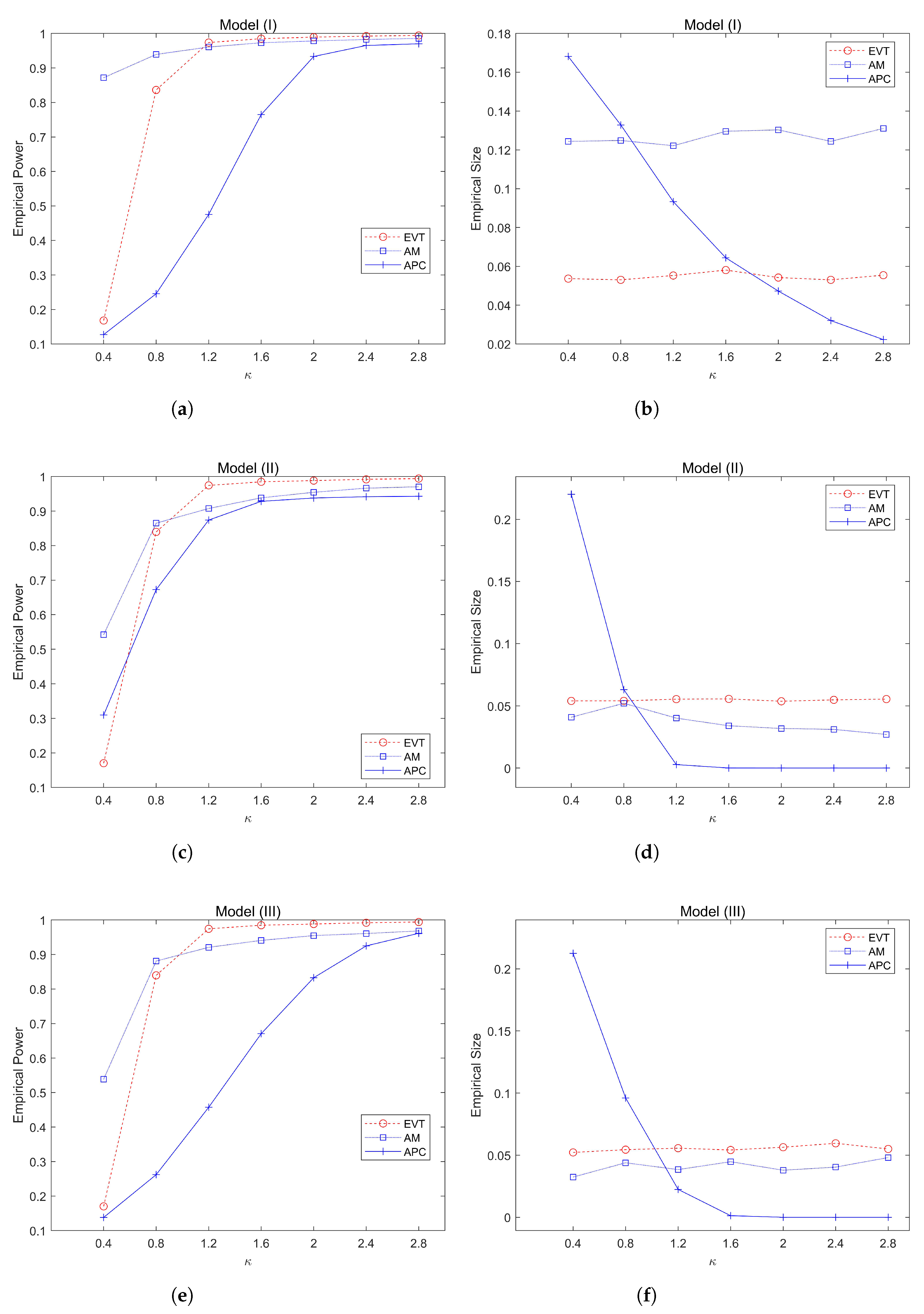
Figure 3 simulates the trend of asymptotic power values and the Type-I error values obtained by three different monitoring methods with the increase of under the three model settings. From Figure 3, it can be seen that on the left side, when or , the power value obtained by the AM method is slightly better than our method, but, when increases to 1.2 or even greater, the power values obtained by our EVT method are significantly better than the other two methods. On the right of Figure 3, it can be seen that the type-I error obtained using the EVT method can be effectively controlled at around 5%, while the AM method cannot control the type-I error effectively in model (I). The results by the APC method also have poor performance,
Table 4 lists the fault diagnosis results of high-dimensional data streams by using different diagnostic methods. We have calculated the values of two main indicators here, one is the correct recognition rate, and the other is the incorrect recognition rate. At the same time, we also considered the value of change point estimation during the online monitoring phase. The results show that as k increases, the change point estimation becomes closer to the true value. Regardless of the proportion of ps being equal to 5%, 10%, or 15%, the EVT method is significantly better than the other two methods. Furthermore, from the diagnostic results, the TP value of the EVT method is close to 100%. It should be noted that the AM method and APC method also have good diagnostic results, but considering the results of point estimation, overall, our method is superior to the other two methods.
Table 4.
Diagnosis accuracy of the proposed procedure, under different choices of and , when , , , and .
Table 4.
Diagnosis accuracy of the proposed procedure, under different choices of and , when , , , and .
| EVT | A-M | APC | |||||||||||||||||||
| TPR | FPR | TPR | FPR | TPR | FPR | ||||||||||||||||
| 1.0 | 212.3 | 99.1 | 0.8 | 213.6 | 100.0 | 0.9 | 210.5 | 71.1 | 4.4 | ||||||||||||
| 5% | 1.5 | 203.3 | 100.0 | 0.8 | 208.6 | 100.0 | 0.9 | 208.1 | 82.1 | 5.4 | |||||||||||
| 2.5 | 201.6 | 100.0 | 0.8 | 206.7 | 100.0 | 0.9 | 206.9 | 85.8 | 7.4 | ||||||||||||
| 1.0 | 206.5 | 99.3 | 1.3 | 209.5 | 100.0 | 0.9 | 209.9 | 84.8 | 10.3 | ||||||||||||
| 10% | 1.5 | 202.1 | 100.0 | 1.4 | 206.1 | 100.0 | 1.0 | 206.7 | 92.8 | 12.9 | |||||||||||
| 2.5 | 201.2 | 100.0 | 1.3 | 204.6 | 100.0 | 0.8 | 206.2 | 94.4 | 15.0 | ||||||||||||
| 1.0 | 204.5 | 99.5 | 1.6 | 209.8 | 100.0 | 0.6 | 208.1 | 91.8 | 12.6 | ||||||||||||
| 15% | 1.5 | 201.4 | 99.7 | 1.7 | 205.0 | 100.0 | 0.9 | 206.2 | 95.7 | 14.2 | |||||||||||
| 2.5 | 200.9 | 100.0 | 1.7 | 204.4 | 100.0 | 0.4 | 205.5 | 96.1 | 13.4 | ||||||||||||
4. Real Data Analysis
In order to verify the effectiveness of the method proposed in this article, we apply the proposed monitoring and diagnostic methods to analyze the real data set. The glass data contains Electron Probe X-ray Microanalysis (EPXMA) intensities for different wavelengths of sixteenth to seventeenth century archaeological glass vessels [21]. We consider this data as a high-dimensional data stream sorted by time points, with 180 time points and each observation containing 750 variables at each time point. Many literatures in abnormal point detection have analyzed this data set, such as Hubert et al. (2005)[22] performed the RobPCA method to analysis the glass data, and identified some row-wised outliers. Hubert et al. (2019)[23] also analyzed this data set by the proposed MacroPCA procedure, and flagged some outlying samples as outliers. In this section, we perform the proposed monitoring and diagnosis procedures on the glass data. Firstly, through preliminary data analysis, we found that 13 variables were missing or invalid. Therefore, for each observation, we first removed 13 variables and left 737 variables for further analysis. Thus, we obtained 180 high-dimensional time series data streams.
In the first stage, our goal is to monitor the time series data stream online and accurately detect abnormal data. So, we selected appropriate parameters and applied the online monitoring strategy proposed in this paper to the data stream, obtaining the results shown in the following figure. The results showed that from time point 57 onwards, there was a loss of control in the data flow, which is consistent with Hubert’s research conclusion.
Figure 4.
The data stream with IC observations (Solid Points), and OC observations (Hollow Circle) when monitoring data streams.
Figure 4.
The data stream with IC observations (Solid Points), and OC observations (Hollow Circle) when monitoring data streams.
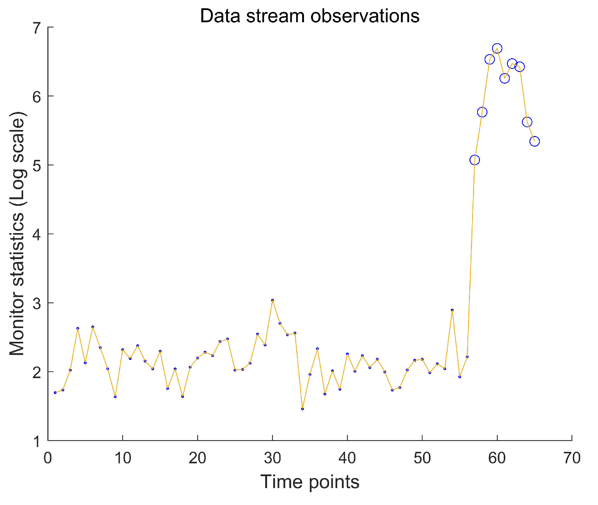
In the second stage, we apply the statistical diagnostic method proposed in this article to further analyze the out of control data stream and identify the variables that cause the data flow to become out of control. During the online monitoring phase, it can be observed that when , the data stream experienced a loss of control. Therefore, we allow the data stream to run for a certain time period (the time length is denoted as 5), and then performed fault diagnosis on the observed values that experienced the loss of control. According to the diagnostic analysis results, when the observation time point of the data stream is greater than 57, out of a total of 737 variables, 36 variables were detected to have undergone abnormal changes, resulting in abnormal drift of the data stream.
5. Conclusions
In this article, we studied the online monitoring and fault diagnosis of high-dimensional data streams. In the first stage, we proposed a online monitoring procedure based on EWMA statistics. As is well known, the EWMA statistic is more sensitive to small changes and it includes information from previous samples. Thus, an EWMA statistic is chosen in this study for monitor high-dimensional stream. We have constructed online monitoring statistics and provided corresponding online monitoring solutions. In the second stage, we constructed diagnostic statistics and provided corresponding statistical diagnostic algorithms. Finally, we validated the effectiveness of the method through numerical simulations and case studies. The simulation results show that our method can quickly and effectively monitor the timing of change points, and can effectively control the rate of erroneous monitoring. Compared with other existing methods, the proposed online monitoring and diagnosis methods have great advantages in controlling type-I errors and also has good power for identifying outlying points, especially for high-dimensional sparse data stream.
References
- Zou, C.; Wang, Z.; Zi, X.; Jiang, W. An efficient online monitoring method for high-dimensional data streams. Technometrics 2015, 57, 374–387.
- Li, J. A two-stage online monitoring procedure for high-dimensional data streams. J. Qual. Technol. 2019, 51, 392–406.
- Li, W.; Xiang, D.; Tsung, F.; Pu, X. A diagnostic procedure for high-dimensional data streams via missed discovery rate control. Technometrics 2020, 62, 84–100.
- Ahmadi-Javid, A.; Ebadi, M. A two-step method for monitoring normally distributed multi-stream processes in high dimensions. Qual. Eng. 2020, 33, 143–155.
- Ebrahimi, S.; Ranjan, C.; Paynabar, K. Monitoring and root-cause diagnostics of high-dimensional data streams. J. Qual. Technol. 2022, 54, 20–43.
- Liu, K.; Mei, Y.; Shi, J. An Adaptive Sampling Strategy for Online High-Dimensional Process Monitoring. Technometrics 2015, 57, 305–319.
- Huang, T.; Kandasamy, N.; Sethu, H.; Stamm, M. An Efficient Strategy for Online Performance Monitoring of Datacenters via Adaptive Sampling. IEEE Trans. Cloud Comput. 2019, 7, 155–169.
- Xiang, D.; Li, W.; Tsung, F.; Pu, X.; Kang, Y. Fault classification for high-dimensional data streams: A directional diagnostic framework based on multiple hypothesis testing. Nav. Res. Logist. (NRL) 2021, 68, 973–987.
- Du, L.; Zou, C. On-line control of false discovery rates for multiple datastreams. J. Stat. Plan. Inference 2018, 194, 1–14.
- Li, J. Efficient global monitoring statistics for high-dimensional data. Qual. Reliab. Eng. Int. 2020, 36, 18–32.
- Xian, X.; Zhang, C.; Bonk, S.; Liu, K. Online monitoring of big data streams: A rank-based sampling algorithm by data augmentation. J. Qual. Technol. 2021, 53, 135–153.
- Xiang, D.; Qiu, P.; Wang, D.; Li, W. Reliable Post-Signal Fault Diagnosis for Correlated High-Dimensional Data Streams. Technometrics 2022, p. 64.
- Colosimo, B.; Jones-Farmer, L.; Megahed, F.; Paynabar, K.; Ranjan, C.; Woodall, W. Statistical Process Monitoring from Industry 2.0 to Industry 4.0: Insights into Research and Practice. Technometrics 2024, 66, 1–35. [CrossRef]
- Hu, X.; Zhao, Y.; Yeganeh, A.; Shongwe, S. Two memory-based monitoring schemes for the ratio of two normal variables in short production runs. Comput. Ind. Eng. 2024, 198, 110690. https://doi.org/10.1016/j.cie.2024.110690. [CrossRef]
- Yoav, B.; Daniel, Y. A multivariate exponentially weighted moving average control chart. Ann. Stat. 2001, 29, 1165–1188.
- Lowry, C.A.; Woodall, W.H.; Champ, C.W.; Rigdon, S.E. A multivariate exponentially weighted moving average control chart. Technometrics 1992, 34, 46–53.
- Feng, L.; Ren, H.; Zou, C. A setwise EWMA scheme for monitoring high-dimensional datastreams. Random Matrices: Theory Appl. 2020, 9, 2050004.
- Cai, T.T.; Liu, W.; Xia, Y. Two-sample test of high dimensional means under dependence. J. R. Stat. Soc. 2014, 76, 349–372.
- Yoav, B.; Yosef, H. Controlling the false discovery rate: A practical and powerful approach to multiple testing. J. R. Stat. Soc. Ser. B (Methodological) 1995, 57, 289–300.
- Du, L.; Guo, X.; Sun, W.; Zou, C. False Discovery Rate Control Under General Dependence By Symmetrized Data Aggregation. J. Am. Stat. Assoc. 2021, 118, 1–34. [CrossRef]
- Lemberge, P.; De Raedt, I.; Janssens, K.H.; Wei, F.; Van Espen, P.J. Quantitative analysis of 16–17th century archaeological glass vessels using PLS regression of EPXMA and μ-XRF data. J. Chemom. A J. Chemom. Soc. 2000, 14, 751–763.
- Hubert, M.; Rousseeuw, P.; Branden, K. ROBPCA: A new approach to robust principal component analysis. Technometrics 2005, 47, 64–79. [CrossRef]
- Hubert, M.; Rousseeuw, P.; Van den Bossche, W. MacroPCA: An All-in-One PCA Method Allowing for Missing Values as Well as Cellwise and Rowwise Outliers. Technometrics 2019, 61, 459–473. [CrossRef]
Figure 1.
The data stream with IC data (gray) and OC data (color), when , , , , . The left subfigure is mean-shift case, and the right subfigure is the covariance shift setting.
Figure 1.
The data stream with IC data (gray) and OC data (color), when , , , , . The left subfigure is mean-shift case, and the right subfigure is the covariance shift setting.
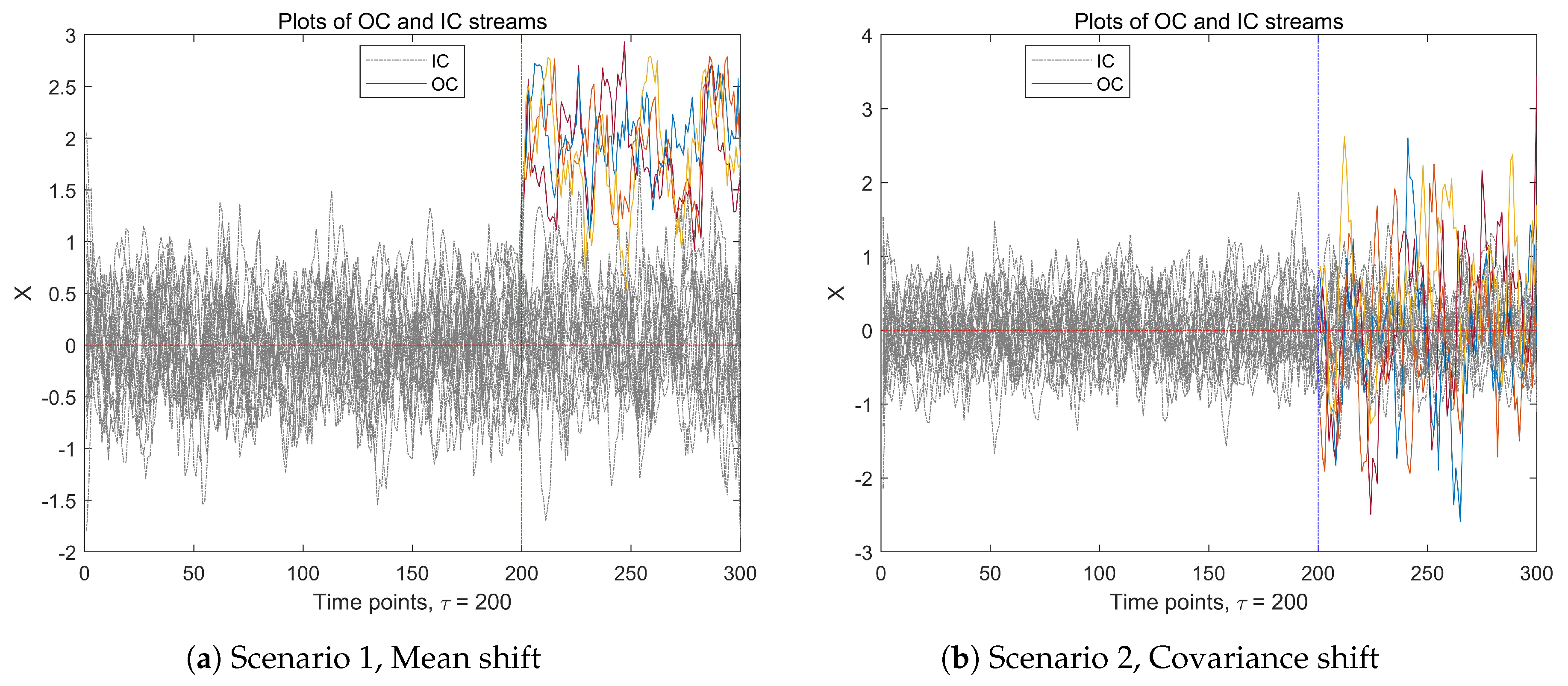
Figure 2.
The change trend of the monitoring statistic value, when , , , . The red dashed line represents the threshold line.
Figure 2.
The change trend of the monitoring statistic value, when , , , . The red dashed line represents the threshold line.
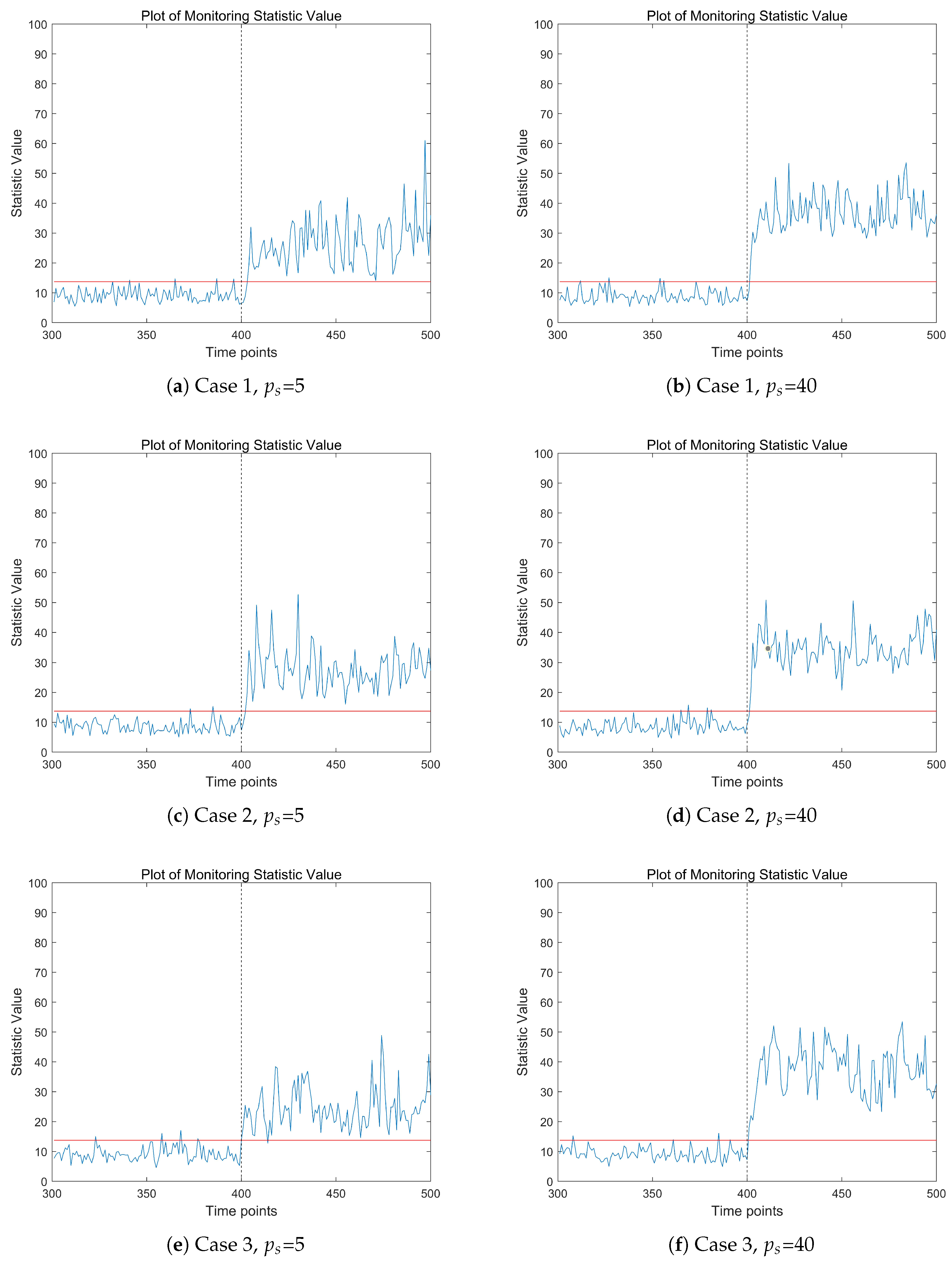
Figure 3.
The change trend of power and size values (%) by various procedures when , , , , with the increase of the parameter .
Figure 3.
The change trend of power and size values (%) by various procedures when , , , , with the increase of the parameter .
Disclaimer/Publisher’s Note: The statements, opinions and data contained in all publications are solely those of the individual author(s) and contributor(s) and not of MDPI and/or the editor(s). MDPI and/or the editor(s) disclaim responsibility for any injury to people or property resulting from any ideas, methods, instructions or products referred to in the content. |
© 2025 by the authors. Licensee MDPI, Basel, Switzerland. This article is an open access article distributed under the terms and conditions of the Creative Commons Attribution (CC BY) license (http://creativecommons.org/licenses/by/4.0/).
Copyright: This open access article is published under a Creative Commons CC BY 4.0 license, which permit the free download, distribution, and reuse, provided that the author and preprint are cited in any reuse.


