
Submitted:
19 January 2025
Posted:
20 January 2025
You are already at the latest version
Abstract
The rapid integration of Machine Learning (ML) in organizational practices has driven demand for substantial computational resources, incurring both high economic costs and environmental impact, particularly from energy consumption. This challenge is amplified in dynamic data environments, where ML models must be frequently retrained to adapt to evolving data patterns. To address this, more sustainable MLOps pipelines are needed that reduce environmental impacts while maintaining model accuracy. In this paper, we propose a model reuse approach based on data similarity metrics, allowing organizations to leverage previously trained models where applicable. We introduce a tailored set of meta-features to characterize data windows, enabling efficient similarity assessment between historical and new data. The effectiveness of the proposed method is validated across multiple ML tasks using cosine and Bray-Curtis distance functions, evaluating both model reuse rates and the performance of reused models relative to newly trained alternatives. The results indicate that the proposed approach can significantly reduce the frequency of model retraining while maintaining or even improving predictive performance, contributing to more resource-efficient and sustainable MLOps practices.
Keywords:
MLOps
; Frugal AI
; Machine Learning
; Meta-Learning
1. Introduction
In recent years, organizations across industries have increasingly adopted Machine Learning (ML) and Artificial Intelligence (AI) to optimize their operations, improve decision-making, and automate tasks [1]. This growing integration into business processes led to a dramatic rise in computational demands, driven not only by the scale of data involved but also by the increasing sophistication of the models being deployed. As ML techniques become a central pillar of modern operations, organizations are either investing in large-scale infrastructure to handle the significant computational requirements necessary for model training and deployment, or relying on cloud infrastructure and services [2].
Contributing to this increase in resource demand is the fact that training ML models has become simpler and more accessible than ever before. Advances in open-source libraries, cloud computing, and powerful pre-trained models have lowered the entry barrier to ML, making it easier for organizations to quickly implement and refine ML solutions [3]. However, this accessibility comes with a trade-off: as more models are developed and deployed, the computational footprint of ML projects continues to grow. The demand for computational resources is particularly steep and continuous in industries where data patterns are dynamic and models must be frequently retrained to adapt to new conditions.
The environmental implications of this trend are substantial. Training state-of-the-art ML models, especially deep neural networks, requires significant energy, leading to an increase in carbon emissions. Some estimates indicate that training a single large language model can emit as much carbon dioxide as five cars over their lifetimes [2]. This environmental cost is further magnified when multiple models are trained for different scenarios or updated frequently in dynamic data environments. Relying heavily on data labeling and continuous model retraining creates an unsustainable cycle of resource consumption, which, if unchecked, can have long-term negative consequences on both economic and environmental fronts [4].
Current practices in ML often default to “throwing resources at the problem,” continually training new models as data changes. While effective in the short term, this approach is neither resource-efficient nor sustainable, given the rising awareness of environmental impacts and the growing demand for responsible AI practices. A more sustainable Machine Learning Operations (MLOps) pipeline is essential: one that minimizes energy use and computational costs while also reducing dependency on human-intensive tasks like data labeling and managing the whole ML cycle. Reducing the need to develop new models in response to data shifts is one of the possible ways towards more efficient and sustainable ML operations.
In this paper, we propose an approach to improve MLOps efficiency by reusing past ML models based on data similarity metrics. The core idea is to assess the similarity between new and historical data to identify cases where previously trained models could be effectively reused. This approach not only saves resources by avoiding redundant model training, but also reduces the reliance on costly and time-intensive data labeling processes, as reusing a model circumvents the need to acquire new labeled datasets. This is especially relevant in the industry, in which the cost of labeling data is often a barrier to technology adoption.
This work is motivated by the needs of the manufacturing domain, particularly in the plastics industry, where quality inspection models are often specific to a product type or version, and where aspects such as machine wear, environmental changes or operator fatigue influence production processes, resulting in data shifts over time. Such variability can quickly render past models obsolete, highlighting the need for an approach that enables model reuse in dynamically changing environments. This work addresses these challenges by presenting a systematic approach to model reuse, providing insights into the potential for resource-efficient MLOps that align with sustainable AI practices [5].
2. Background
2.1. Machine Learning Operations
MLOps refers to the practice of deploying, managing, and maintaining machine learning models in production environments. It integrates DevOps principles with machine learning to streamline the model life-cycle from development to deployment, including continuous integration and delivery (CI/CD) pipelines, automated testing, version control, monitoring, and governance [6].
MLOps aims to enhance the efficiency and reliability of machine learning workflows by ensuring consistent and reproducible results. Key approaches to achieving effective MLOps include infrastructure automation, robust data management, model versioning, and real-time monitoring to promptly detect and resolve issues. These practices are essential for scaling machine learning solutions and maintaining their performance in real-world applications [7].
Despite its potential, many industrial machine learning projects fail to progress from proof of concept to production due to challenges in automation and operationalization [8]. The paradigm of MLOps addresses these issues by providing best practices, sets of concepts, and a development culture to automate and operate ML systems effectively [8].
The standardization and automation of the machine learning pipeline is also an opportunity to introduce sustainable practices and approaches such as those proposed in this paper which, if seamlessly integrated into the MLOps pipeline, will become a part of the organizational culture regarding machine learning, and maximize the benefits regarding sustainability.
2.2. Frugal AI
The Frugal AI vision focuses on creating AI solutions that are resource-efficient, cost-effective, and accessible. The goal is to achieve high performance while minimizing the use of data, computational power, time, or human resources. This approach is essential in industries where data is scarce, costly, or rapidly changing, making traditional AI methods less viable. Frugal AI techniques include computational optimizations such as model pruning, quantization, distillation, and leveraging pre-trained models through transfer learning [9]. Continuous learning methods such as active learning and rotation-based techniques also play a role [10].
On the data side, Frugal AI uses data reduction and generation strategies, including sampling methods, PCA, data augmentation, and synthetic data creation. These methods ensure efficient use of resources while maintaining or improving AI model performance. Additionally, Frugal AI aligns with Green AI principles by optimizing algorithms, improving hardware efficiency, and adopting sustainable data management practices to reduce environmental impacts [11].
2.3. Concept Drift
In the context of a dataset, concept drift refers to changes in the statistical properties of the target variable, which machine learning models aim to predict over time. These changes can degrade model performance as the underlying data distribution evolves, and they can occur at different speeds, severity and distributions [12]. Concept drift poses a significant challenge in maintaining accurate and reliable models, particularly in dynamic environments. There are several types of concept drift including sudden drift (abrupt changes in data distribution), gradual drift (slow and incremental changes over time), incremental drift (continuous but gradual changes) or recurrent drift (cyclical changes where old patterns reappear).
When addressing concept drift, organizations traditionally rely on strategies such as frequent model retraining, adaptive algorithms, and monitoring systems, to promptly detect and respond to changes. The impact of concept drift on model performance has been notably observed in clinical applications such as sepsis prediction, where data drift can significantly affect the accuracy of machine learning models [13].
Due to its nature, concept drift might have a significant impact on resource consumption in machine learning, due to the need to frequently train new models, which often also imply new labeled data. Approaches such as the one proposed in this paper may minimize this impact, more so in cases of recurrent drift, as repeating patterns in the data increase the likeliness of successfully retrieving a past machine learning model.
2.4. Meta-Learning
Meta-learning, or "learning to learn," aims to improve the efficiency and performance of machine learning algorithms by leveraging knowledge from prior learning tasks. It reduces the need for extensive trial-and-error by utilizing meta-data, which includes performance metrics of algorithms or dataset characteristics. Meta-features are specific characteristics of datasets that aid in this process. Examples of meta-features include simple statistical properties, advanced statistical measures, information-theoretic metrics, and model-based features. Rivolli et al. [14] categorized meta-features into several types: simple, statistical, information-theoretic, model-based, and landmarking meta-features.
Examples of meta-learning applications include hyperparameter optimization, model selection, and algorithm recommendation. In the past, we have worked extensively on meta-learning, which culminated in the development of an algorithm recommendation system that significantly reduced the time and resources spent on selecting an appropriate algorithm and doing hyperparameter tuning [15]. In this paper we build on this past experience.
3. Methodology
The main objective of this research is to propose an approach to reuse existing machine learning models to minimize the use of computational resources, taking advantage of the similarity between old and new data, and the respective models. This approach was developed to be used in various scenarios, but mainly in data streaming scenarios where data evolves over time, a phenomenon known as concept drift. By reusing models that were previously trained on similar data, it is possible to significantly reduce the need to (re)train new models from scratch, thus saving time and computational power. This section begins by briefly summarizing the methodology followed, which is then further detailed below.
The methodology was developed and validated using a large group of publicly available datasets, which were divided into fixed-size chunks to simulate data streaming over time. For each data block, a comprehensive set of meta-features is extracted using the PyMFE library [16]. These meta-features provide a detailed characterization of each data block across multiple dimensions, such as general characteristics, statistical properties, information theoretic metrics, model-based characteristics, and reference measures.
By characterizing data blocks with meta-features, we transform them into a suitable format for measuring similarity. Meta-feature vectors serve as a compact representation of data blocks, capturing essential information about their statistical and structural properties.
After the meta-features are extracted, the distance between data blocks is calculated using these meta-feature vectors. This distance calculation encodes the similarity between the new data block and those in the historic model pool, and it is based on that distance that a certain model is reused or not. The rest of this section describes the two distance metrics tested (Section 3.1), the process for finding a reduced set of meta-features suitable for retrieving past models (Section 3.2), and the process through which models are reused (Section 3.3).
3.1. Distance Metrics
Calculating the distance between two vectors is a key element in this work. In this section, we describe two widely used vector distance metrics, which we compared to implement the proposed approach.
3.1.1. Bray-Curtis Dissimilarity
In this work, the Bray-Curtis dissimilarity measures the proportional differences between two data blocks. It is calculated as depicted in equation 1.
where and are the values of the i-th feature in two data blocks being compared.
Under the Bray-Curtis approach, the distance between two feature vectors is computed based on the direct comparison of each pair of values in the vector, as depicted in Figure 1.
The Bray-Curtis dissimilarity thus measures the proportional differences between the data blocks based on the feature comparisons. Figure 2 depicts, through heatmaps and using the Bray-Curtis dissimilarity metric, the distance between each pair of data blocks in six datasets. The top row consists of real-world datasets, while the bottom row consists of synthetic datasets. In these images, a dark-blue color indicates a very small distance, whereas a dark red indicates a large distance. The diagonal has a zero distance as it represents the distance between each block and itself. The values of distance using the Bray-Curtis dissimilarity range between 0 (equal vectors) and 1 (completely different vectors).
3.1.2. Cosine Similarity
Cosine similarity, on the other hand, measures the cosine of the angle between two vectors in a multidimensional space. It is calculated as depicted in equation 2.
where is the dot product of the vectors, and and are the magnitudes of the vectors.
The intuition behind the cosine similarity is depicted in Figure 3, for a bi-dimensional feature space. In this representation, each arrow represents the feature vector of one data block, both starting at the origin. The closer the vectors are to each other, the more similar they are. The same principle applies in a higher-dimensional feature space, but its visualization becomes impracticable. Cosine similarity ranges from -1 to 1, where 1 indicates identical vectors, 0 indicates orthogonality (no similarity), and -1 indicates completely opposite vectors.
Figure 4 visually depicts the differences between the same datasets and blocks of data used in Figure 2, but now using the cosine similarity. While the heatmaps are similar to some extent, it is also visible that the notion of distance varies according to the distance metric used. The choice might thus impact the performance of model reuse policies, and several metrics should be tested and assessed.
3.2. Meta-Feature Selection
Given the variety of meta-features that can be considered, one prior aspect to model reuse is the selection of the set of meta-features to use. On the one hand, some of these meta-features might not be relevant at all and introduce entropy in the process. On the other hand, we want to find the minimum set of features that allow to efficiently reuse models. This has to do with computational efficiency aspects, as the extraction of meta-features from a block of data also has a computational cost. While extracting features generally has a much smaller computational cost than training a model, a large set of meta-features might reduce the advantages of the proposed approach. Thus, the selection of an appropriate set of meta-features is a key step in this process.
The methodology employed to achieve this is depicted in Figure 5. It consists of two main phases: selection and validation.
The first phase consisted in pre-selecting a set of meta-features for posterior validation. In this process, we used several datasets (already shown in Figure 2 and Figure 4), both real-world and synthetic, exhibiting different types of concept drift (gradual and abrupt). Real-world datasets include Airlines, CovType, and Electricity (Elec), while synthetic datasets include Agrawal-abrupt, Hyper_f, and Sea_a [17,18,19].
Each dataset was segmented into an arbitrary fixed-sized set of sequential blocks, based on its size. From each block, and based on our own previous work and experience [15], we extracted an initial set of 66 meta-features using the PyMFE library [16] and trained a Random Forest model with default settings using the scikit-learn library (v1.4). Performance metrics such as accuracy, precision, and recall were collected for each model, forming six meta-datasets. Each meta-dataset contained rows corresponding to the blocks of the original datasets, linking block characteristics (meta-features) to model performance.
Subsequently, Random Forest models (which we deem meta-models) were trained on each meta-dataset, with the goal of predicting accuracy based on the meta-features. The relative importance of each meta-feature in predicting model accuracy was assessed, and those with at least 1% relative importance (when compared to the most important meta-feature) were selected. This selection process was repeated across the six meta-datasets, and meta-features identified as important in at least three out of the six cases were pre-selected.
To ensure robustness and mitigate the effects of randomness, this process was repeated ten times. Each iteration resulted in a different reduced set of meta-features, ranging in number between five to ten. Finally, the ten meta-features with the highest selection frequency across all iterations were chosen. Table 1 presents these meta-features along with their frequencies.
The second phase consisted on the validation of the selected meta-features, specifically in their suitability for model reuse. In this phase, twenty-four datasets were used, which did not include the previous 6. Following a similar procedure to the first phase, each dataset was divided into fixed-sized blocks, and meta-features (both the initial set of 66 and the reduced set of 10) were extracted. One model was trained for each block of data, which was then (both the blocks of data and the models) randomly assigned to one of two groups.
The first group is the model pool, which simulates the existing past models and their corresponding blocks of training data. The second group is the validation group, which simulates future blocks of data that are arriving, and the corresponding models that would be trained on these data. The goal is to compare the would-be models with the retrieved models, in order to assess the quality of the retrieval approach.
For each block in the validation group (representing new incoming data), the closest block from the pool was identified. We then retrieved the corresponding model from the pool, and compared its predictive performance on the new block of data against the performance of its respective model. That is, the model that would have been trained with that new data. We did this using both sets of meta-features (10 and 66), in order to assess both groups of meta-features in terms of number of meta-features (complexity) vs. predictive performance of the reused models.
Since the size of the pool might affect the results, as larger pools will potentially hold better candidate models, the experiments were conducted with varying pool sizes (10% to 50% of the blocks) and repeated five times to account for randomness in the distribution of data and models between the pool and validation groups. The effects of both groups of meta-features on the quality of the retrieved models, discussed in detail in Section 4, indicates that the smaller set of 10 meta-features performs at a comparable degree to the larger set, while being computationally less intensive.
3.3. Model Reuse
This section describes the proposed methodology for reusing machine learning models based on similarity between blocks of data, measured using the selected set of meta-features. In this process of model reuse there are three key elements, which are described next.
The pool consists of a group triplets of size n, in which n represents the number of data blocks received in the past via streaming, and for which machine learning models have been trained. Thus, and , and represent, respectively, the model trained with block i, the performance metrics of (e.g. accuracy, precision, recall) and the vector of meta-features of block i. There is also a temporal relationship between these triplets, so that comes before in time than . While the order in which data blocks are received (and models trained) is not currently relevant, in the future we will experiment with more complex distance functions, which might include the freshness of the data.
The second relevant element is the distance function to be used to estimate the similarity between sets of data. As previously described, each block of data is characterized by a vector of meta-features, that is intended to represent core properties of the data. As shown in Section 3.1, namely through Figure 2 and Figure 4, the function used influences how data similarity is measured. Some aspects to bear in mind when selecting the distance function are that each dimension in the feature vector might have very different ranges of values (with some contributing proportionally more to the total distance than others), and that one may want to attribute different weights to each dimension depending, for example, on the relative frequency of each one during the selection process (Table 1). Testing and evaluating different distance functions is thus paramount.
Finally, there is also the need to define a maximum distance threshold. While the approach consists in selecting the closest model, or more precisely the model whose training data is closest to the current block of data, it may happen that the closes block of data is not close enough. This maximum distance threshold thus defines the point after which, instead of reusing a model, we choose to train a new one, based on the new data. The selection of this threshold significantly impacts the performance of the approach. Setting it to a low value will lead to a very low model reuse rate, but a higher confidence on the quality of the models reused. Conversely, it this threshold is very high, the number of reused models will rise significantly, but eventually their average predictive performance will be lower. This threshold cannot also be defined in an absolute manner, as it depends on several aspects including the distance function used or the characteristics of the data stream. Instead, it should be defined empirically.
Finally, with these three elements, the problem of model reuse can be formalized as follows: the goal is to select the model from the pool such that the distance between and (the meta-features vector of model ) is minimized. That is,
where represents a distance function between meta-feature vectors, and k is the index of the model in the pool with the smallest distance to .
Thus, the selected model is given by:
To test the assumption that similarity metrics combined with meta-features are a good proxy to predict model performance, we devised the methodology depicted in Figure 6, which was validated with 24 datasets and which is similar to the methodology followed for selecting the reduced set of meta-features.
For each dataset, the process begins with splitting each dataset into fixed-sized blocks, to simulate windows of streaming data. The size of each block was defined arbitrarily based on the size of the dataset. For each block, a machine learning model was trained and its performance metrics recorded. Specifically, we used Random Forest classifiers with scikit-learn v1.4 and the default hyper-parameters. It is important to note that no effort was made to optimize each individual ML model, as the primary goal of this work is to validate the proposed approach rather than to find the optimum model for each specific use case. For each block of data we also extracted the meta-features vector using the PyMFE package (v0.4.3). This results in the previously described group of triplets in the shape of .
The next step involved splitting this group of triplets into two sub-groups: the pool sub-group (representing the historic of data and models that exists at time t) and the validation sub-group, which represents all the data that arrived after time t, and the corresponding models. We tested pools of different sizes, ranging from 10% to 50% of the total data, at 10% intervals.
For each data block in the validation group, which represents newly arrived data, we retrieved the closest block from the pool. As described previously, this was done taking into consideration the distance between the vectors of meta-features and each of the two distance metrics used, for comparison. In essence, once the closest block of data to be reused was identified, if its distance to the new block was smaller than a predefined threshold, the corresponding model from the pool was reused. Otherwise, a new model was trained on the new block. Actually, a new model is also trained when a model is reused from the pool, in order to allow a performance comparison between both. However, in a real use-case models would only be trained when no model in the pool is similar enough.
To evaluate the idea of selecting past machine learning models based on the similarity of current data to the training data, we ran a parallel experiment in which models were randomly selected from the pool. That is, we aimed to assess whether selecting models from an historic pool according to data similarity and meta-features is significantly better than selecting them randomly from the same pool.
The performance of the selected models (distance-based: Bray-Curtis and cosine similarity) on the new data block was assessed using the Root Mean Squared Error (RMSE) metric. To minimize the effect of randomness, each experiment was repeated five times for each dataset and pool size, resulting in a total of 5 * 5 (pool sizes) * 6 (datasets) = 150 experiments. This procedure was repeated for each of the five different distance metrics, leading to a total of 750 experiments.
To summarize, our methodology employs meta-feature extraction and similarity measurement to facilitate the efficient reuse of machine learning models in data streaming scenarios. By leveraging both Bray-Curtis dissimilarity or cosine similarity metrics, we aim to identify and utilize previously trained models on similar data blocks, thereby reducing the computational resources required for model (re)train.
4. Results
This section presents the outcomes of validating the reduced group of meta-features, and of subsequently using them to reuse past machine learning models. The section is therefore structured into two primary subsections: Meta-feature Selection and Model Reuse.
We consider two main metrics to assess the performance of the proposed approaches in what concerns retrieving and reusing past models: correlation of accuracies and average distance of accuracies. The correlation of accuracies measures reliability, through the degree to which the accuracies of reused models when predicting on new data align with those of the models that would be trained on the same new data. The average distance of accuracies evaluates prediction accuracy, through the absolute differences in performance.
4.1. Meta-feature selection
This section presents the results of validating our methodology with 24 datasets, distinct from those used in selecting the reduced set of meta-features. We evaluate our approach using two key indicators: (1) the correlation between the accuracy of each model in the validation group (the new model, trained on the new data) and the accuracy of the model reused from the pool on the same new block of data, and (2) the Mean Absolute Difference (MAD) between the accuracy of models in the validation group and the reused models. The correlation metric assesses how well-aligned the retrieved models are with models trained on the new data, while MAD measures the performance gap between them. Table 2 summarizes the findings for the 24 datasets with a pool size of 20%.
Overall, for a 20% pool size, using the selected 10 meta-features preserved a strong correlation compared to the full set of 66 meta-features across various datasets, independently of the distance function used. In some cases, such as Social_Network_Ads, bank_10000, and hyper_f, the reduced set even outperformed the full set. However, there were instances, such as cardio_vascular_10000 and pima_indians_diabetes, where using only 10 meta-features resulted in poorer correlation and/or increased error. These results suggest that a case-by-case selection of meta-features may be necessary for different use cases, as outlined in our methodology. For a 20% pool size, the reduction to 10 meta-features outperformed the full set of 66 in terms of correlation for 62.5% of the datasets and achieved a smaller MAD in 37.5% of the datasets.
It is also useful to visually depict the results of the proposed approach. Figure 7 shows the accuracy of the specifically trained models against the retrieved model, using the reduced set of meta-features and the Bray-Curtis distance, for six datasets. It can be seen how the retrieved models are generally well aligned with the actual models that would be trained on the new block of data. Figure 8 is similar, but the retrieval was done using cosine similarity rather than the Bray-Curtis distance. It can be seen that there are datasets for which it is generally harder to reuse models (e.g. CovType), and also that Bray-Curtis seems a better distance metric to reuse models than cosine similarity, as corroborated by Table 3.
Table 3 summarizes the outcomes for varying pool percentages from 10% to 50% using different meta-feature sets. On average, the identified group 10 meta-features achieves better correlation between validation and reused model accuracies in 2 out of 5 pool sizes compared to using all 66 features. It also yields a lower average MSE in 4 out of 5 cases. The analysis of datasets on an individual basis shows that the group of 10 features outperform the full set in terms of correlation for 54-63% of problems, depending on the pool size. A similar 38-46% advantage is observed for the average MSE. This confirms a reduced meta-feature set can effectively characterize datasets for the purpose of model retrieval, while lowering computational overhead. When comparing both distance metrics investigated, it is clear from the table that across all 24 datasets and 5 pool sizes tested, Bray-Curtis generally holds better results than cosine similarity.
4.2. Model reuse
While the previous section analyzed the performance of both distance metrics investigated in reusing models, this section adopts a more realistic approach to the problem by looking at it as a time-series one. That is, while to validate the reduced set of meta-features we selected data and models at random to attribute them to both pools (historic and validation), we now take the streaming data in the order it was produced, as would have happened in reality. At a given point in time t, we thus assume that every model trained until is available to be reused. In each new timestamp t in which a new window of data is available, we decide whether to reuse a model or to train a new one. The criteria for doing so has to do with the maximum distance threshold and the distance between each past block of data and the current one. The only exception to this is the first iteration, in which there are no past models, so a new model is always trained.
In this case, we look at two main metrics. First, we want to calculate the percentage of models that were effectively reused, as this provides insights into the computational resources that are saved when not training models. Second, we look at the quality of the retrieved models when predicting on the new data, when compared with the models that would actually be trained on the new data. This means that, for validation purposes, we train one model for each block of data. However, in a real use-case, there would be no model being trained when an old one is retrieved, which would result in the saving of computational resources, time, and eventually human resources as well if data labeling was necessary.
The effect of the proposed methodology on model reuse can be intuitively perceived in Figure 9 to Figure 12. In these figures, each line represents the performance of models over time for a given machine learning problem. The blue line can be seen as the baseline, and it shows the RMSE over time when specific models are trained for each new block of data. The green line, on the other hand, shows the RMSE over time of the proposed approach, in which some models are reused. These lines overlap when there is no good candidate model to be reused (according to the threshold defined). When a model is reused, its RMSE measured on the new data is displayed, as well as its id. This is shown as a label above the red dot. That is, a label for Model n indicates that, at that moment in the stream, model n was reused rather than a new model being trained. Model indexes start at 0.
These figures also highlight the effect of using different thresholds: the higher the threshold, the more models are reused, as expected. However, the quality of the models may be lower. While the results are more precisely detailed in the Tables below, it can be seen that the proposed approach results in models that are generally aligned with the traditional approach, in which one model is trained for each new block of data.
More specifically, Figure 9 and Figure 10 show the performance of the proposed approach for two datasets (Airlines and Sea) for varying threshold levels, defined empirically, and using the cosine distance to retrieve models.
Figure 9.
Plot of average RMSE values per threshold and model index using the Cosine method (Airlines Dataset)
Figure 9.
Plot of average RMSE values per threshold and model index using the Cosine method (Airlines Dataset)
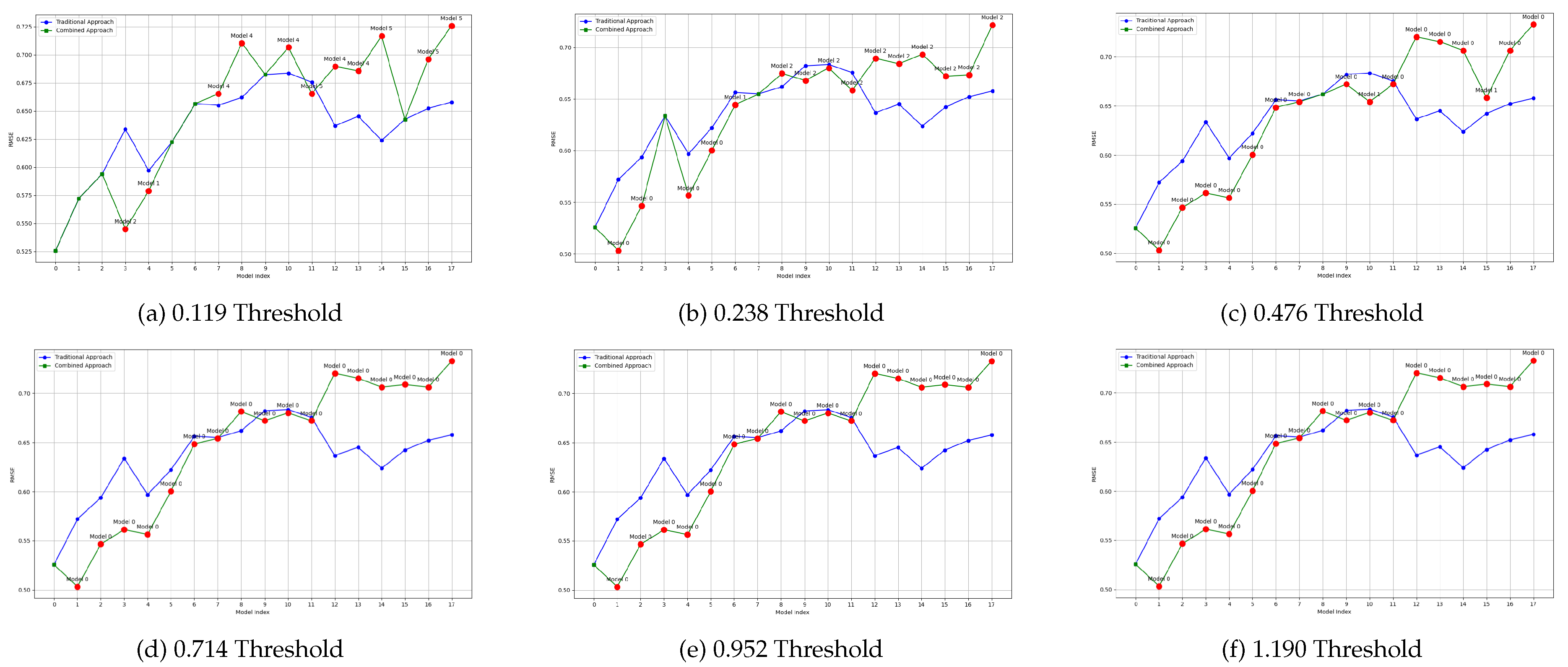
Figure 10.
Plot of average RMSE values per threshold and model index using Cosine method (Sea Dataset)
Figure 10.
Plot of average RMSE values per threshold and model index using Cosine method (Sea Dataset)
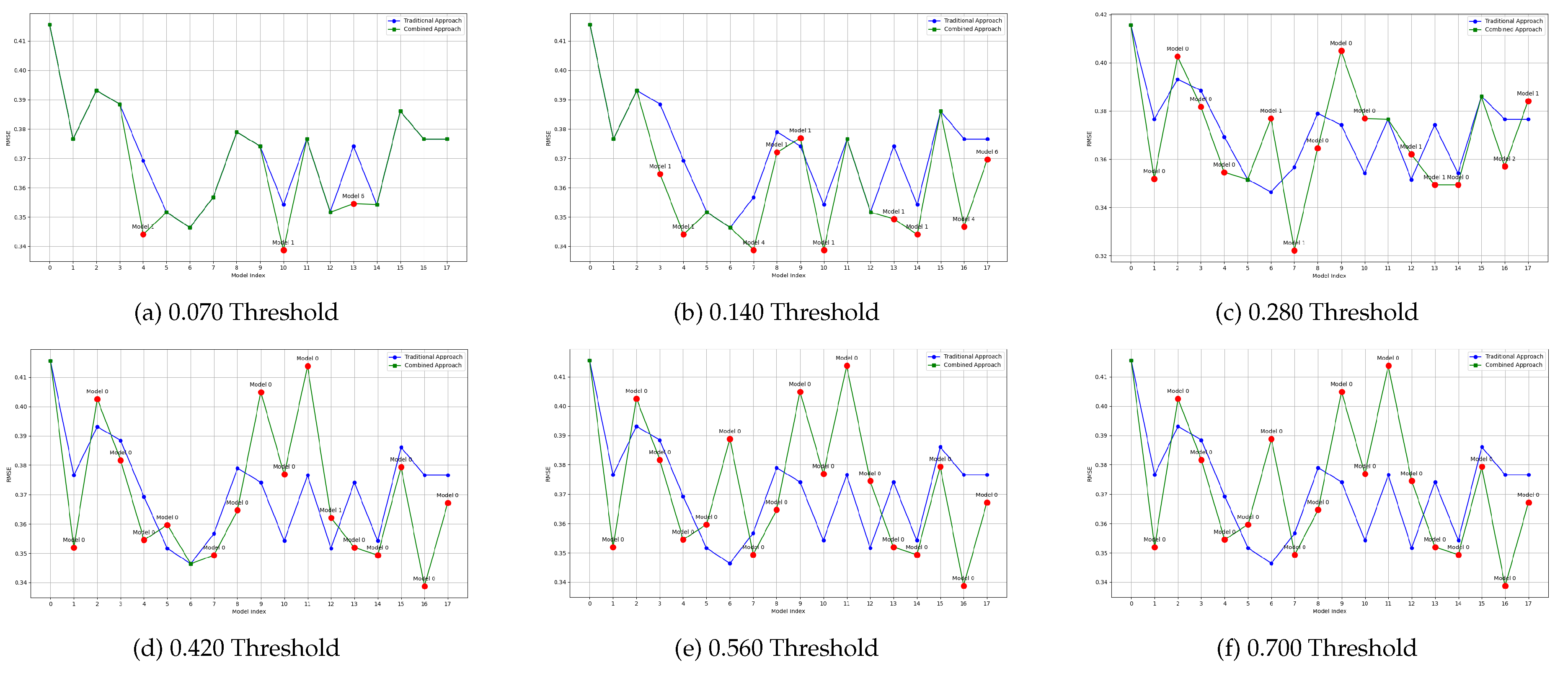
Figure 11 and Figure 12 show the results for the same datasets, but using the Bray-Curtis distance to determine which models to reuse. As previously mentioned, it can be seen how more models are reused when a higher threshold is used. It can also be seen, independently of the distance metric used, that the models reused are in some case better than the actual models, and in other cases worse. More detail is thus provided in the Tables below.
Figure 11.
Plot of average RMSE values per threshold and model index using the Bray-Curtis method (Airlines Dataset)
Figure 11.
Plot of average RMSE values per threshold and model index using the Bray-Curtis method (Airlines Dataset)
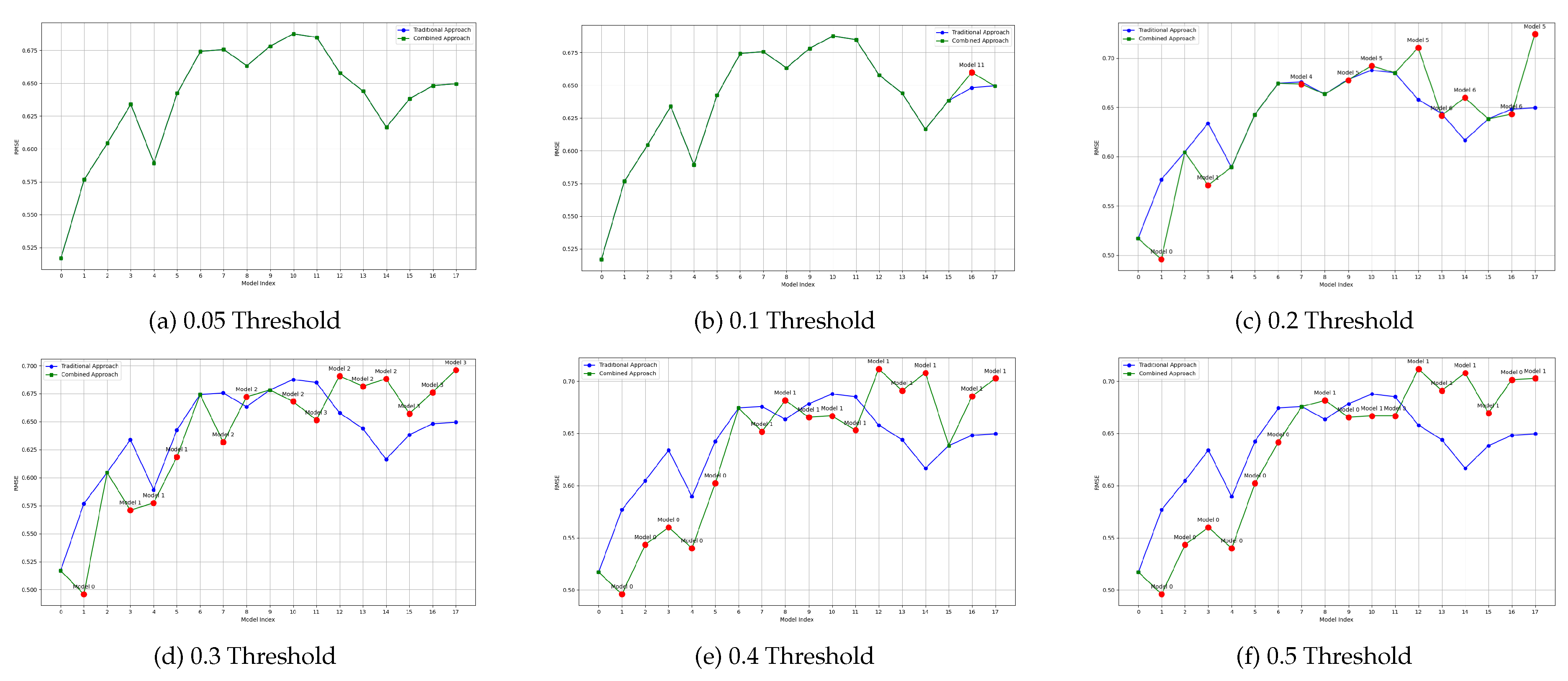
Figure 12.
Plot of average RMSE values per threshold and model index using the Bray-Curtis method (Sea Dataset)
Figure 12.
Plot of average RMSE values per threshold and model index using the Bray-Curtis method (Sea Dataset)
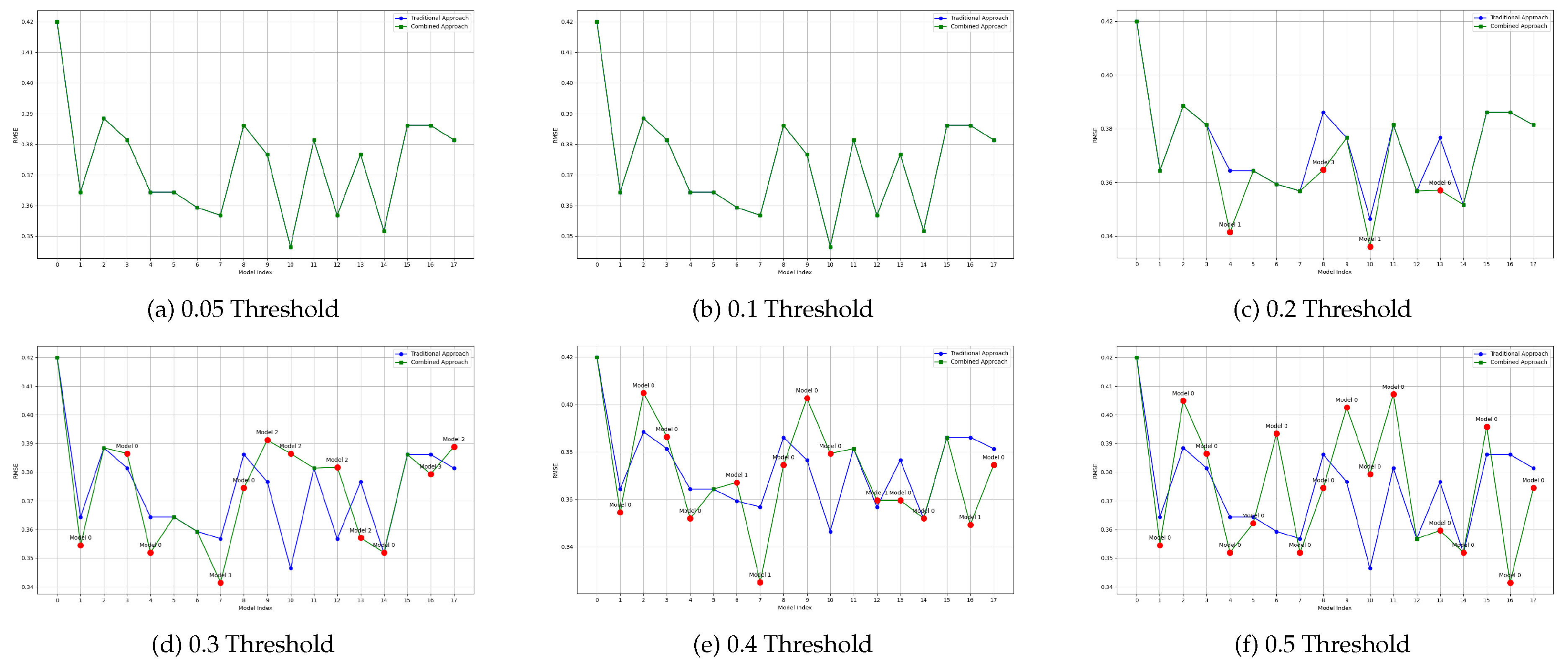
Table 4, Table 5, Table 6 and Table 7 summarize the results of this evaluation, for the two datasets that were also depicted in Figure 9 to Figure 12. In this case, since the goal is to evaluate the quality of the retrieved models, we compare the proposed approach with a random selection of a past model. That is, in both cases we select a model from the past pool, but we compare selecting it randomly with selecting it based on the proposed approach: using the reduced set of meta-features and one of the two distance metrics investigated.
Table 4 and Table 5 summarize the results for different levels of threshold for the Airlines dataset, using the cosine and Bray-Curtis distance metrics, respectively. When using the Cosine distance, the retrieved models have a very similar performance to that of models retrieved randomly. However, when using the Bray-Curtis distance, the proposed approach outperforms the random selection of models in 4 out of the six thresholds tested. The rate of models reused is however slightly smaller in the second case, ranging between 0% and 88.89% (Bray-Curtis) against 61.11% to 94.44% (Cosine similarity).
The proposed approach for reusing models in data streaming scenarios has proven promising, as it often matches or outperforms the performance of traditional approaches. This validates the hypothesis that data similarity metrics can be a good predictor of model performance, and a computationally inexpensive way of selecting the most promising group of pre-trained models. Nonetheless, as has been shown, it must be kept in mind that the results depend largely on the configuration used, and especially on a balance between the number of reused models and their computational performance. The ideal values to achieve this balance must be, in a first instance, searched through empirical processes, such as the one described here, and depend also on the constraints of the organization (e.g. the available computational resources or budget).
5. Conclusions and Future work
In this paper, we addressed the increasingly relevant need for sustainable and resource-efficient MLOps practices in light of the growing computational and environmental demands associated with machine learning. By proposing a novel approach that leverages data similarity metrics to enable the reuse of previously trained models on-the-fly, we take a step forward towards minimizing the need for training new models and, consequently, to minimizing the need for labeling data by organizations, which often represents an adoption barrier or a cutoff in model quality.
With the reuse of models, machine learning pipelines also become more autonomous and less dependent on human activities and expertise, as each model that is reused is a model that did not need to be trained, and whose data did not need to be labeled.
All of this relies on using meta-features that accurately describe the properties of data and its relationship with the downstream model quality. As such, the process of meta-feature extraction also has a computational cost which must not be discarded. Since one of the goals of this work is to improve sustainability indicators, we also set out to identify a reduced of meta-features that could accurately achieve this. We have shown that a reduction from the original 66 to a set of 10 meta-features maintained or slightly improved the performance of the retrieved models, showing that this reduced set of meta-features was enough.
Lastly, another relevant factor that was studied is the function used to compute the distance between meta-feature vectors, i.e., between windows of data. We have compared the performance of the cosine and Bray-Curtis distance, and concluded that Bray-Curtis is the best approach.
We tested and validated this work on a comprehensive set of streaming and batch datasets, some of them with concept drift, both natural and synthetic. We did not always achieve better results than with traditional approaches, but it can be stated that in the majority of the cases, results were equivalent or better. However, it must also be stated that achieving better results than traditional approaches was never the main goal. The main goal was to achieve equal or better results, while minimizing the number of machine learning models trained. And we consider that goal achieved since in most of the cases, the number of models trained can be significantly reduced, often by 70% to 90%, without a significant loss in predictive performance. These results thus show that data distance metrics can indeed be used as a proxy to reuse previously trained models.
Despite the fact that this approach was extensively validated, there are still a few limitations. First and foremost, it is clear that this approach must be tailored to each specific use-case, especially in what concerns the definition of the threshold to retrieve past models. This threshold is paramount as it defines the percentage of models that are reused, as well as their expected quality, since less similar data blocks will, in principle, hold less suited models. Nonetheless, the empiric process described here, in which several thresholds are objectively evaluated, can be followed in other use-cases to identify the best threshold to use.
Another limitation not yet addressed is that of the size of the pool. The solution described in this paper assumes that the pool can grow forever. This is not realistic as there are resource limitations for the amount of models that can be stored, and also since as the model pool grows, so too does the computational complexity for choosing a model. Thus, in future work, we are implementing this process for pools of limited size, in which the models of the pool are managed according to their age or their inter-similarity.
Moreover, we are also working on migrating to pool of models to an ensemble of models. That is, instead of maintaining a pool of models but only using the most suitable one at each moment, we are using all the models in the pool in the form of an ensemble. This significantly improves the predictive quality of the models, at the cost of some computational complexity. In this version, the size of the pool / ensemble becomes even more important, and it will be up to the organization to decide between one approach or the other, depending on resource and costs constraints.
The final limitation that is currently being addressed is that of deciding when to run the process of selecting a new model. In this work, we trigger the process at regular intervals, for each window of data. However, there are cases in which the statistical patterns of the data being generated did not change significantly, so there’s no need to change the model. We are currently incorporating outlier and concept drift detection, so that the process is only triggered when significant changes to the data are detected, further optimizing resource consumption.
All in all, we believe that the proposed approach is a promising one to minimize resource consumption and human intervention in modern MLOps, making them more efficient and sustainable.
Author Contributions
Conceptualization, D.C. and B.S.; methodology, D.C.; software, E.P. and D.T.; validation, D.C. and R.M.; data curation, E.P. and D.T.; writing—original draft preparation, D.C. and R.M.; writing—review and editing, B.S. and R.M.; visualization, E.P. and D.T.; supervision, D.C.; funding acquisition, D.C. and B.S. All authors have read and agreed to the published version of the manuscript.
Funding
This work has been supported by the European Union under the Next Generation EU, through a grant of the Portuguese Republic’s Recovery and Resilience Plan (PRR) Partnership Agreement, within the scope of the project PRODUTECH R3 – "Agenda Mobilizadora da Fileira das Tecnologias de Produção para a Reindustrialização", Total project investment: 166.988.013,71 Euros; Total Grant: 97.111.730,27 Euros.
Conflicts of Interest
The authors declare no conflicts of interest. The funders had no role in the design of the study; in the collection, analyses, or interpretation of data; in the writing of the manuscript; or in the decision to publish the results.
References
- Jordan, M.I.; Mitchell, T.M. Machine learning: Trends, perspectives, and prospects. Science 2015, 349, 255–260. [Google Scholar] [CrossRef] [PubMed]
- Strubell, E.; Ganesh, A.; McCallum, A. Energy and policy considerations for modern deep learning research. In Proceedings of the Proceedings of the AAAI conference on artificial intelligence, 2020, Vol. 34, pp. 13693–13696.
- LeCun, Y.; Bengio, Y.; Hinton, G. Deep learning. nature 2015, 521, 436–444. [Google Scholar] [CrossRef] [PubMed]
- Henderson, P.; Hu, J.; Romoff, J.; Brunskill, E.; Jurafsky, D.; Pineau, J. Towards the systematic reporting of the energy and carbon footprints of machine learning. Journal of Machine Learning Research 2020, 21, 1–43. [Google Scholar]
- Govindan, K. How artificial intelligence drives sustainable frugal innovation: A multitheoretical perspective. IEEE Transactions on Engineering Management 2022, 71, 638–655. [Google Scholar] [CrossRef]
- Gupta, P.; Bagchi, A. MLOps: Machine Learning Operations. In Essentials of Python for Artificial Intelligence and Machine Learning; Springer Nature Switzerland: Cham, 2024; pp. 489–518. [CrossRef]
- Ruf, P.; Madan, M.; Reich, C.; Ould-Abdeslam, D. Demystifying mlops and presenting a recipe for the selection of open-source tools. Applied Sciences 2021, 11, 8861. [Google Scholar] [CrossRef]
- Kreuzberger, D.; Kühl, N.; Hirschl, S. Machine Learning Operations (MLOps): Overview, Definition, and Architecture. IEEE Access 2023, 11, 31866–31879. [Google Scholar] [CrossRef]
- Kim, J.; Chang, S.; Kwak, N. PQK: model compression via pruning, quantization, and knowledge distillation. arXiv 2021, arXiv:2106.14681 2021. [Google Scholar]
- Liu, B. Lifelong machine learning: a paradigm for continuous learning. Frontiers of Computer Science 2017, 11, 359–361. [Google Scholar] [CrossRef]
- Bol’on-Canedo, V.; Mor’an-Fern’andez, L.; Cancela, B.; Alonso-Betanzos, A. A review of green artificial intelligence: Towards a more sustainable future. Neurocomputing, 1280. [Google Scholar]
- Suárez-Cetrulo, A.L.; Quintana, D.; Cervantes, A. A survey on machine learning for recurring concept drifting data streams. Expert Systems with Applications 2023, 213, 118934. [Google Scholar] [CrossRef]
- Rahmani, K.; Thapa, R.; Tsou, P.; Casie Chetty, S.; Barnes, G.; Lam, C.; Foon Tso, C. Assessing the effects of data drift on the performance of machine learning models used in clinical sepsis prediction. International Journal of Medical Informatics 2023, 173, 104930. [Google Scholar] [CrossRef] [PubMed]
- Rivolli, A.; Garcia, L.P.; Soares, C.; Vanschoren, J.; de Carvalho, A.C. Characterizing classification datasets: a study of meta-features for meta-learning. arXiv 2018, arXiv:1808.10406 2018. [Google Scholar]
- Palumbo, G.; Carneiro, D.; Guimares, M.; Alves, V.; Novais, P. Algorithm recommendation and performance prediction using meta-learning. International journal of neural systems 2023, 33, 2350011. [Google Scholar] [CrossRef] [PubMed]
- Alcobaça, E.; Siqueira, F.; Rivolli, A.; Garcia, L.P.F.; Oliva, J.T.; de Carvalho, A.C.P.L.F. MFE: Towards reproducible meta-feature extraction. Journal of Machine Learning Research 2020, 21, 1–5. [Google Scholar]
- Gomes, H.M.; Bifet, A.; Read, J.; Barddal, J.P.; Enembreck, F.; Pfharinger, B.; Holmes, G.; Abdessalem, T. Adaptive random forests for evolving data stream classification. Machine Learning 2017. [Google Scholar] [CrossRef]
- Blackard, J.A.; Dean, D.J. Comparative accuracies of artificial neural networks and discriminant analysis in predicting forest cover types from cartographic variables. Computers and Electronics in Agriculture 2000, 24, 131–151. [Google Scholar] [CrossRef]
- Harries, M.; Wales, N.S. Splice-2 comparative evaluation: Electricity pricing, 1999.
Figure 1.
Intuition behind the Bray-Curtis Dissimilarity.
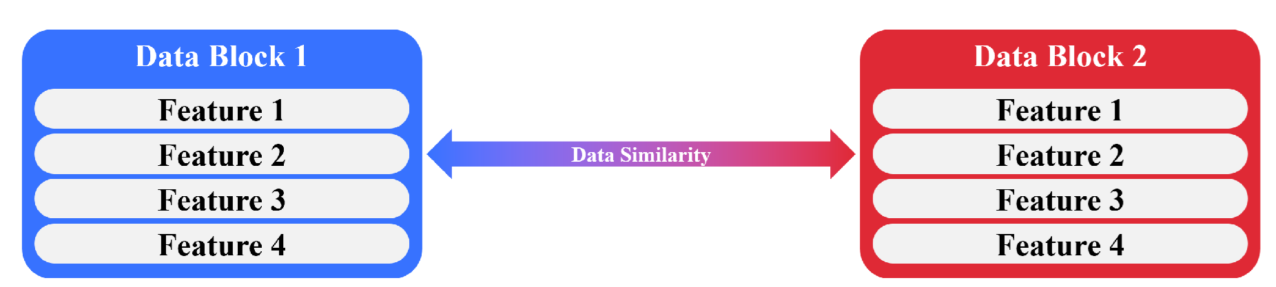
Figure 2.
Heatmap visualization of distances between blocks of data for both real-world (upper row) and synthetic (lower row) datasets using the Bray-Curtis dissimilarity.
Figure 2.
Heatmap visualization of distances between blocks of data for both real-world (upper row) and synthetic (lower row) datasets using the Bray-Curtis dissimilarity.
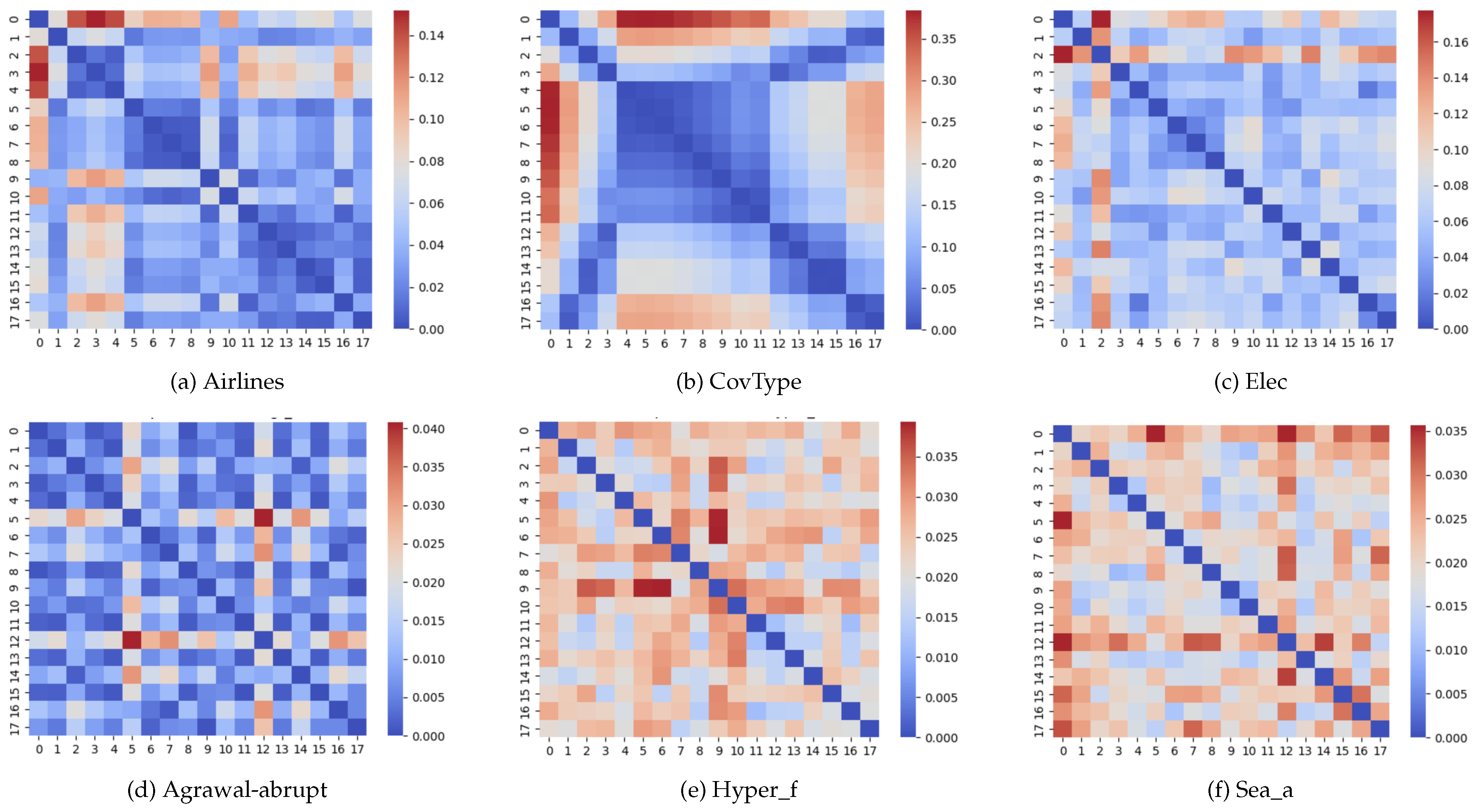
Figure 3.
Intuition behind the cosine similarity.
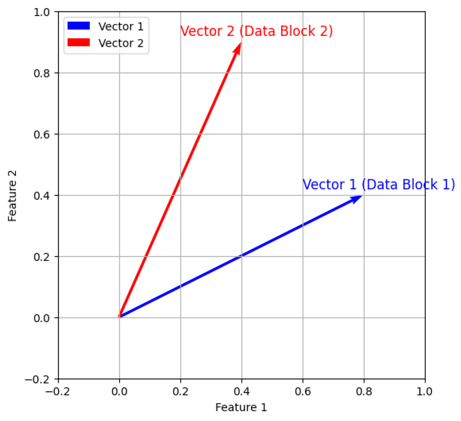
Figure 4.
Heatmap visualization of distances between blocks of data for both real-world (upper row) and synthetic (lower row) datasets using the cosine distance.
Figure 4.
Heatmap visualization of distances between blocks of data for both real-world (upper row) and synthetic (lower row) datasets using the cosine distance.
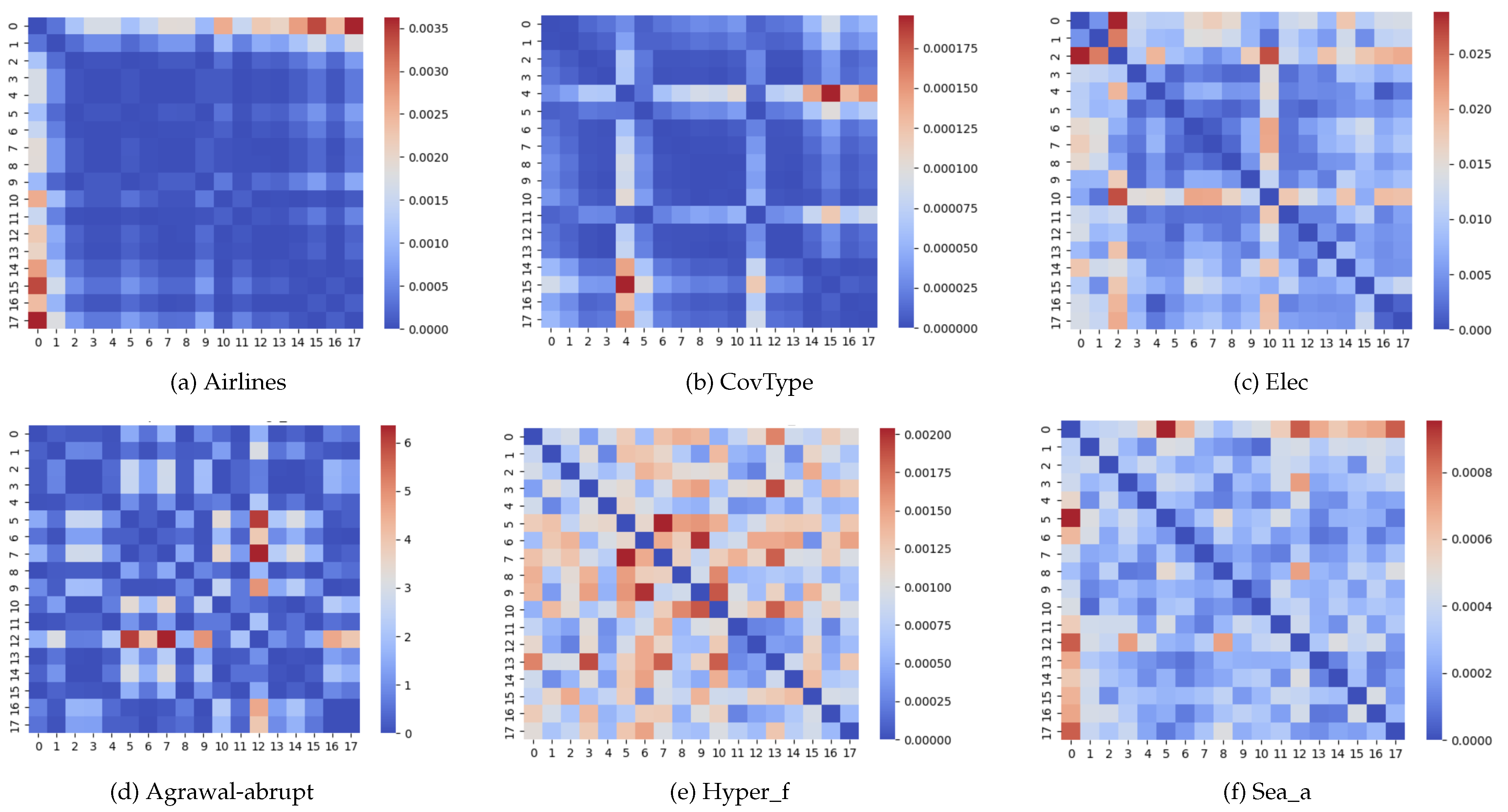
Figure 5.
Methodology followed for selecting and validating a reduced set of meta-features.
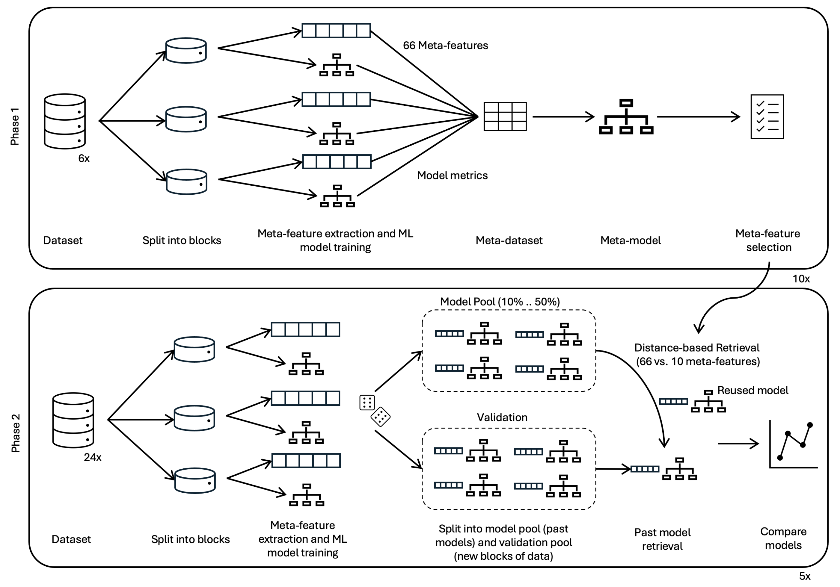
Figure 6.
Process followed to validate the proposed approach.
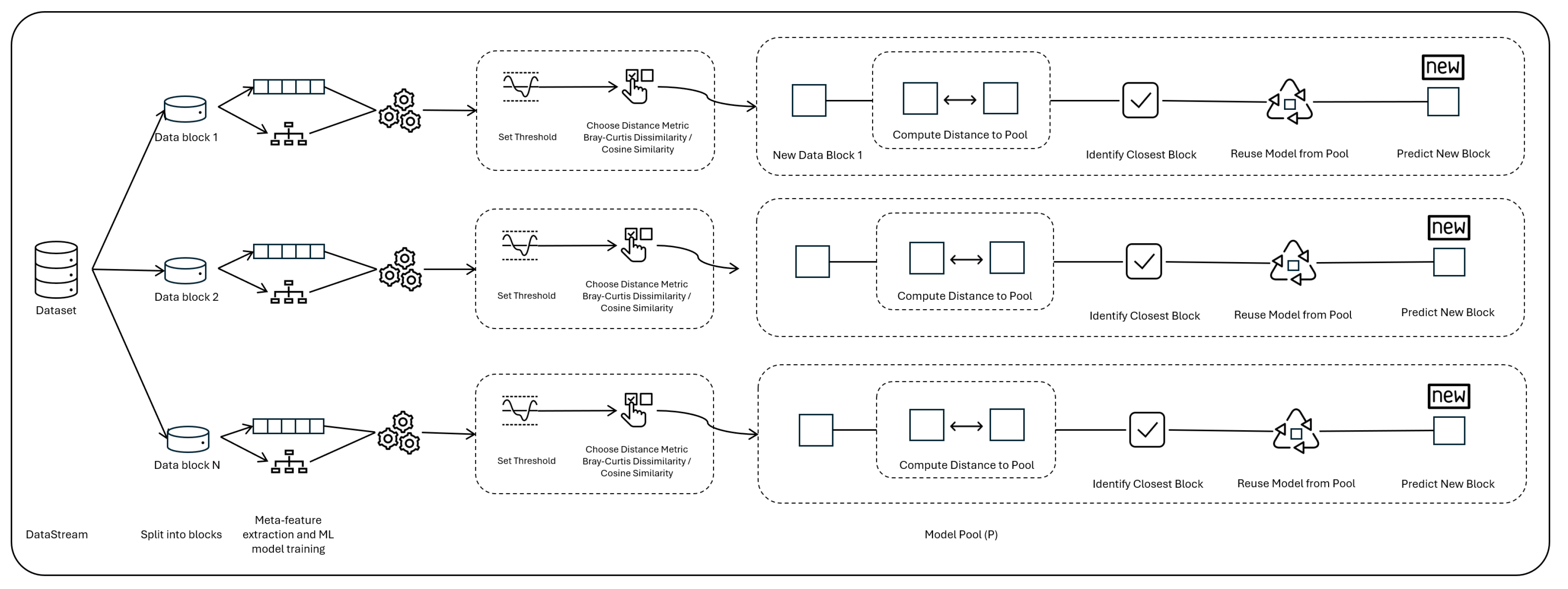
Figure 7.
Comparison of the accuracy of a specifically trained model vs. the accuracy of a reused model (using the Bray-Curtis distance) for three real (first row) and synthetic (second row) datasets.
Figure 7.
Comparison of the accuracy of a specifically trained model vs. the accuracy of a reused model (using the Bray-Curtis distance) for three real (first row) and synthetic (second row) datasets.
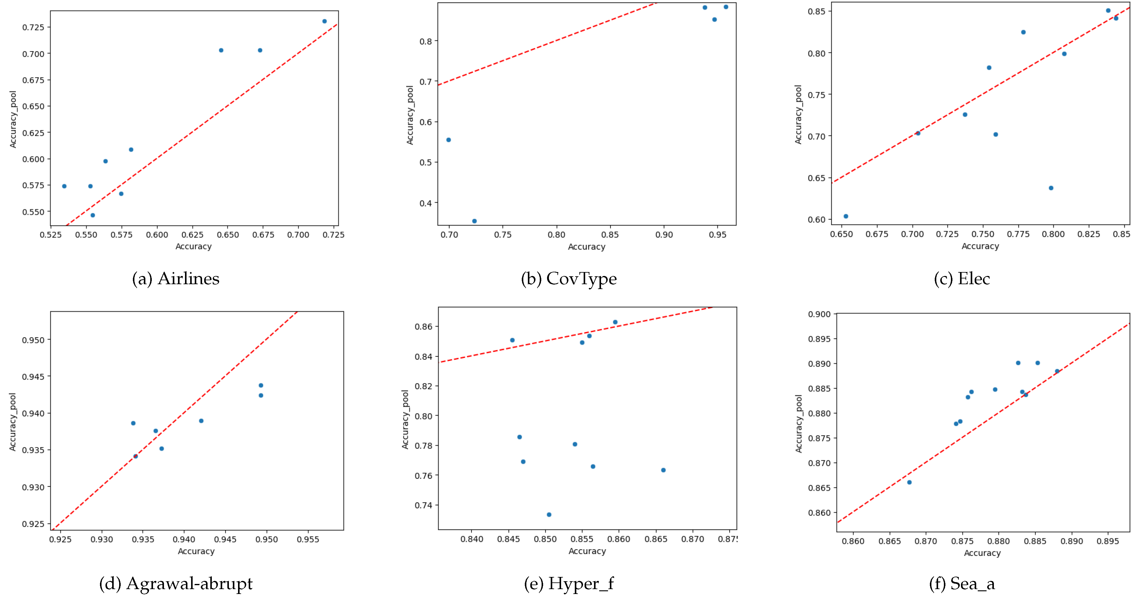
Figure 8.
Comparison of the accuracy of a specifically trained model vs. the accuracy of a reused model (using the cosine distance) for three real (first row) and synthetic (second row) datasets.
Figure 8.
Comparison of the accuracy of a specifically trained model vs. the accuracy of a reused model (using the cosine distance) for three real (first row) and synthetic (second row) datasets.
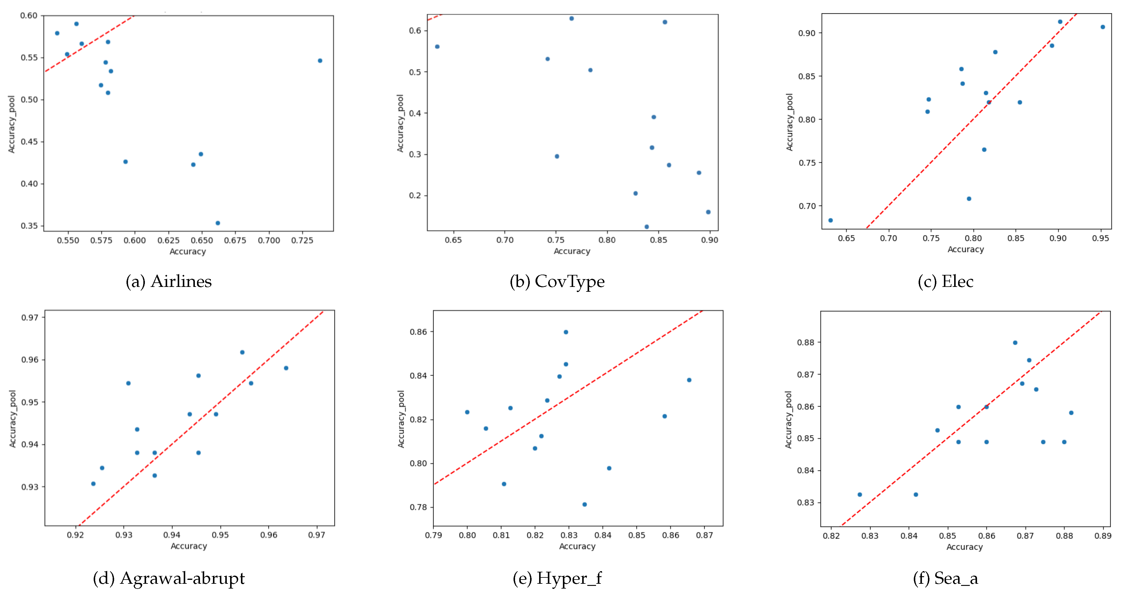

Table 1.
Reduced set of 10 selected meta-features and their frequency over the 10 iterations of the process.
Table 1.
Reduced set of 10 selected meta-features and their frequency over the 10 iterations of the process.
| Meta-feature | Description | Frequency |
|---|---|---|
| nre | Normalized relative entropy | 10 |
| one_nn.mean | Performance of the 1-Nearest Neighbor classifier | 9 |
| freq_class.sd | Relative frequency of each distinct class | 9 |
| linear_discr.sd | Performance of the Linear Discriminant classifier | 9 |
| elite_nn.mean | Performance of Elite Nearest Neighbor | 7 |
| naive_bayes.sd | Performance of the Naive Bayes classifier | 5 |
| linear_discr.mean | Performance of the Linear Discriminant classifier | 4 |
| best_node.mean | Performance of the best single decision tree node | 4 |
| naive_bayes.mean | Performance of the Naive Bayes classifier | 2 |
| mean.sd | Mean value of each attribute (standard deviation) | 2 |
Table 2.
Performance Comparison between the two sets of meta-features and the two distance metrics used, for a pool size of 20%.
Table 2.
Performance Comparison between the two sets of meta-features and the two distance metrics used, for a pool size of 20%.
| Dataset | 66 Meta-Feat. | 10 Meta-Feat. (BC) | 10 Meta-Feat. (Cos) | |||
|---|---|---|---|---|---|---|
| Corr | MAD | Corr | MAD | Corr | MAD | |
| airlines | 0.85 | 0.04 | 0.80 | 0.04 | 0.21 | 0.08 |
| elec | 0.54 | 0.06 | 0.60 | 0.01 | -0.43 | 0.19 |
| general_data | 0.32 | 0.07 | 0.46 | 0.05 | 0.02 | 0.06 |
| german_credit | 0.69 | 0.05 | 0.80 | 0.06 | 0.09 | 0.07 |
| SN_Ads | 0.81 | 0.05 | 0.91 | 0.01 | 0.44 | 0.20 |
| agr_a | 0.84 | 0.01 | 0.87 | 0.01 | 0.84 | 0.01 |
| cardio_10k | 0.74 | 0.01 | 0.40 | 0.07 | 0.54 | 0.02 |
| pima | 0.74 | 0.06 | 0.48 | 0.06 | 0.50 | 0.05 |
| sea_a | 0.43 | 0.01 | 0.85 | 0.05 | 0.80 | 0.01 |
| wpbc | 0.71 | 0.13 | 0.07 | 0.03 | 0.92 | 0.08 |
| abalone | 0.42 | 0.04 | 0.51 | 0.19 | 0.86 | 0.02 |
| cardio_dv3 | 0.72 | 0.01 | 0.73 | 0.02 | 0.59 | 0.02 |
| bank_10k | 0.08 | 0.78 | 0.85 | 0.01 | -0.36 | 0.15 |
| covtype | 0.57 | 0.27 | -0.12 | 0.08 | -0.37 | 0.48 |
| wine_red | 0.74 | 0.06 | 0.34 | 0.11 | 0.78 | 0.08 |
| credit_1k | 0.37 | 0.03 | 0.69 | 0.01 | -0.28 | 0.05 |
| wine_green | -0.31 | 0.08 | 0.02 | 0.02 | 0.85 | 0.05 |
| Housing | -0.05 | 0.18 | 0.79 | 0.01 | -0.04 | 0.14 |
| fram_heart | 0.71 | 0.02 | 0.58 | 0.06 | 0.69 | 0.01 |
| hyper_f | 0.35 | 0.02 | 0.74 | 0.02 | -0.19 | 0.02 |
| HR_Attr | 0.93 | 0.01 | 0.86 | 0.02 | 0.95 | 0.01 |
| wdbc | 0.20 | 0.05 | 0.29 | 0.38 | 0.35 | 0.08 |
| world_food | -0.07 | 0.03 | 0.03 | 0.09 | -0.13 | 0.07 |
| calories_9k | 0.73 | 0.01 | 0.02 | 0.06 | 0.87 | 0.01 |
Table 3.
Summary of the results for different pool sizes when comparing 66 vs. 10 meta-features.
| Pool Size | 66 Meta-Feat. | 10 Meta-Feat. (BC) | 10 Meta-Feat. (Cos) | |||
|---|---|---|---|---|---|---|
| Corr | MAD | Corr | MAD | Corr | MAD | |
| 10% | 0.45 | 0.067 | 0.37 | 0.07 | 0.47 | 0.08 |
| 20% | 0.50 | 0.09 | 0.52 | 0.06 | 0.35 | 0.08 |
| 30% | 0.53 | 0.064 | 0.42 | 0.062 | 0.43 | 0.10 |
| 40% | 0.45 | 0.062 | 0.47 | 0.06 | 0.36 | 0.11 |
| 50% | 0.58 | 0.09 | 0.51 | 0.06 | 0.40 | 0.12 |
Table 4.
Average RMSE values per threshold using Cosine method (Airlines Dataset)
| Threshold | Random | Proposed | Avg. Difference | Models Reused (%) | ||
|---|---|---|---|---|---|---|
| Avg | Sum | Avg | Sum | |||
| 0.12 | 0.63 | 11.42 | 0.65 | 11.68 | -0.01 | 61.11 |
| 0.24 | 0.64 | 11.48 | 0.00 | 83.33 | ||
| 0.48 | 0.64 | 11.50 | 0.00 | 88.89 | ||
| 0.71 | 0.64 | 11.59 | -0.01 | 94.44 | ||
| 0.95 | 0.64 | 11.59 | -0.01 | 94.44 | ||
| 1.19 | 0.64 | 11.59 | -0.01 | 94.44 | ||
Table 5.
Average RMSE values per threshold using Braycurtis method (Airlines Dataset)
| Threshold | Random | Proposed | Avg. Difference | Models Reused (%) | ||
|---|---|---|---|---|---|---|
| Avg | Sum | Avg | Sum | |||
| 0.05 | 0.64 | 11.48 | 0.64 | 11.48 | 0.00 | 0.00 |
| 0.10 | 0.64 | 11.49 | 0.00 | 5.55 | ||
| 0.20 | 0.64 | 11.50 | 0.00 | 55.55 | ||
| 0.30 | 0.64 | 11.45 | 0.00 | 77.78 | ||
| 0.40 | 0.63 | 11.39 | 0.01 | 83.33 | ||
| 0.50 | 0.64 | 11.44 | 0.00 | 88.89 | ||
Table 6.
Average RMSE values per threshold using Cosine method (Sea Dataset)
| Threshold | Random | Proposed | Avg. Difference | Models Reused (%) | ||
|---|---|---|---|---|---|---|
| Avg | Sum | Avg | Sum | |||
| 0.07 | 0.37 | 6.70 | 0.37 | 6.64 | 0.00 | 16.67 |
| 0.14 | 0.36 | 6.54 | 0.01 | 55.55 | ||
| 0.28 | 0.37 | 6.67 | 0.00 | 77.78 | ||
| 0.42 | 0.37 | 6.67 | 0.00 | 88.89 | ||
| 0.56 | 0.37 | 6.73 | 0.00 | 94.44 | ||
| 0.70 | 0.37 | 6.73 | 0.00 | 94.44 | ||
Table 7.
Average RMSE values per threshold using BrayCurtis method (Sea Dataset)
| Threshold | Random | Proposed | Avg. Difference | Models Reused (%) | ||
|---|---|---|---|---|---|---|
| Avg | Sum | Avg | Sum | |||
| 0.05 | 0.37 | 6.73 | 0.37 | 6.73 | 0.00 | 0.00 |
| 0.10 | 0.37 | 6.73 | 0.00 | 0.00 | ||
| 0.20 | 0.37 | 6.65 | 0.00 | 22.22 | ||
| 0.30 | 0.37 | 6.74 | 0.00 | 66.67 | ||
| 0.40 | 0.37 | 6.69 | 0.00 | 77.78 | ||
| 0.50 | 0.38 | 6.77 | 0.00 | 88.89 | ||
Disclaimer/Publisher’s Note: The statements, opinions and data contained in all publications are solely those of the individual author(s) and contributor(s) and not of MDPI and/or the editor(s). MDPI and/or the editor(s) disclaim responsibility for any injury to people or property resulting from any ideas, methods, instructions or products referred to in the content. |
© 2025 by the authors. Licensee MDPI, Basel, Switzerland. This article is an open access article distributed under the terms and conditions of the Creative Commons Attribution (CC BY) license (http://creativecommons.org/licenses/by/4.0/).
Copyright: This open access article is published under a Creative Commons CC BY 4.0 license, which permit the free download, distribution, and reuse, provided that the author and preprint are cited in any reuse.


