1. Introduction
The uniaxial compressive strength (UCS) of rock materials is among the most critical parameters in geotechnical and civil engineering because it directly influences the design of excavations, tunnels, retaining walls, and other load-bearing structures [
1]. In regions such as Seybaplaya in Campeche, Mexico—where sedimentary rock units, particularly limestone and clay, are widely used as construction aggregates—accurate determination of UCS is essential for ensuring both structural stability and cost-effectiveness [
2]. Although conventional UCS testing procedures (e.g., ASTM D7012-10) provide reliable measurements, they are frequently time-consuming, expensive, and logistically challenging, especially for heterogeneous or weak rock materials that can be difficult to core and prepare to standard specifications [
3,
4].
Given these challenges, indirect approaches that rely on more easily measurable or estimable properties have gained increased attention. Water content, porosity, and density are among the most influential parameters in shaping the mechanical behavior of sedimentary rocks [
5,
6]. Elevated water content can weaken the internal grain bonds and promote microfracture propagation, while higher porosity typically reduces the load-bearing capacity by increasing void space and stress concentrations [
2]. In contrast, density often has a positive correlation with UCS, reflecting tighter grain packing and a more cohesive mineral matrix. However, straightforward regression models linking any single parameter to UCS often fail to capture the intrinsic complexities of carbonate formations, particularly in karstic settings. Local heterogeneities—including variable mineralogy, clay seams, microcracks, and partial saturation—can lead to scattered data and relatively low coefficients of determination when relying on purely linear or polynomial correlations [
2,
7].
To address these limitations, machine learning (ML) techniques—especially artificial neural networks (ANNs)—have emerged as robust tools for predicting compressive strength from multiple rock properties [
8]. Unlike traditional regression approaches that assume a fixed functional form, ANNs can adapt their internal structure to uncover intricate, nonlinear relationships among water content, porosity, density, and UCS. This makes them especially valuable for heterogeneous geologic environments such as Seybaplaya, where karst features, blasting-induced microfractures, and geological discontinuities complicate direct correlations. By learning patterns from available experimental datasets, neural networks can reduce the uncertainty associated with single-variable or bivariate regressions and often yield higher predictive accuracy [
9].
Recent work on Seybaplaya bank rocks demonstrates the importance of multivariate approaches. For example, Naal-Pech et al. [
2] reported that increasing porosity generally lowers compressive strength, whereas higher rock density is correlated with enhanced load-bearing capacity. Water content also exhibits a pronounced effect on rock strength, partly because of chemical weakening and microcrack development. Traditional empirical models may only partially reflect these interactions, sometimes producing large prediction errors or low correlation coefficients. By systematically incorporating multiple variables within an ANN framework, it becomes possible to capture complex or higher-order interactions, thereby improving overall prediction fidelity for both laboratory-scale and field-scale applications [
6].
In this study, we propose a neural-network-based multivariate model to predict the UCS of Seybaplaya bank rocks using water content, porosity, and density as primary input variables. We build upon prior research that has explored linear, polynomial, and other empirical correlations in Southeastern Mexico, aiming to demonstrate that machine-learning tools can offer more accurate, robust estimates under varying geological and hydrogeological conditions. Specifically, this manuscript seeks to:
Quantify the individual and combined effects of water content, porosity, and density on compressive strength in Seybaplaya bank rocks.
Develop and validate an ANN model to capture the nonlinear interactions among these parameters.
Compare the predictive performance of the ANN approach against conventional regression models.
Provide a practical decision-support tool for engineers, geoscientists, and heritage conservationists when selecting rock materials or planning excavation activities in karstic limestone regions.
By encompassing a wide range of conditions—such as partial to fully saturated states, variable clay content, and diverse microfracture intensities—our neural-network-based model offers a more holistic and flexible strategy for predicting UCS. The results are expected to facilitate more cost-effective site investigations, guide better-informed blasting or drilling programs, and enhance confidence in the stability analysis of critical infrastructures. Moreover, although focused on Seybaplaya bank rocks, the proposed methodology can be adapted to similar geological settings worldwide, underlining the broader relevance and applicability of ML-driven approaches in modern rock mechanics.
2. Related Works
2.1. Empirical and Regression-Based Approaches
A considerable body of literature has explored empirical correlations between compressive strength and intrinsic rock properties [
1,
2,
3]. For example, Peng and Zhang [
2] evaluated sandstone, shale, limestone, and dolomite formations in the Gulf of Mexico, establishing linear, logarithmic, or exponential relationships. Their findings generally indicated that
porosity negatively impacts uniaxial compressive strength (UCS), while
density tends to correlate positively with rock strength. Nevertheless, such empirical models can perform poorly for heterogeneous materials or in situations where
water saturation significantly modifies a rock’s mechanical response [
4].
Freyburg [
5] and McNally [
6] also proposed predictive equations for compressive strength based on ultrasonic velocity and porosity in various sedimentary rocks (e.g., sandstone and coal measures). Although such models offered valuable insights for more uniform lithologies, they frequently assume minimal mineralogical or textural variability—an assumption that does not align well with the complex geology found in Seybaplaya, where mixed carbonate and clay minerals complicate direct application of generic correlations [
1].
2.2. Influence of Rock Properties on Compressive Strength
Several studies have highlighted how
water content,
porosity, and
density individually affect compressive strength [
2,
7,
8,
9]. Small variations in water content can induce measurable changes in UCS, particularly in partially to fully saturated rock samples [
10]. Elevated water content reduces effective cohesion and increases pore pressure, promoting microcrack propagation and thereby weakening the rock matrix [
2,
7].
Porosity also plays a decisive role: higher porosity often correlates with lower UCS because it introduces additional voids and potential crack paths [
8]. At the same time, density—which is closely tied to porosity—generally reflects the rock’s load-bearing capacity [
11]. Rocks of higher density tend to exhibit fewer voids, enhancing their mechanical strength [
12]. However, as Lal [
13] emphasized, porosity-related parameters must be contextualized within a rock’s mineralogy and textural characteristics. Consequently,
direct correlations such as “UCS vs. porosity” or “UCS vs. density” may prove insufficient for karst-affected formations like those in Seybaplaya, where partial saturation and heterogeneous microstructures introduce significant scatter in measurements [
1,
14].
2.3. Neural Networks for Predictive Modeling in Geomechanics
While traditional regression-based methods remain common, they often struggle with capturing the highly
non-linear and multivariate interactions found in real-world geologic systems [
2,
15]. This limitation has spurred a growing interest in
machine learning (ML) approaches—particularly
artificial neural networks (ANNs)—which do not presume any specific functional form and are thus well-suited to modeling complex or hidden relationships [
15,
16]. By incorporating multiple input variables such as water content, porosity, density, and even sonic velocity, neural networks can learn to predict UCS more accurately than polynomial or linear regression in many cases [
3,
17].
For instance, Gokceoglu [
15] showed that ANN models outperformed regression analyses for a diverse set of rock types, leveraging petrographic and physical data to capture intricate variable interactions. Likewise, Galván and Restrepo [
9] demonstrated that integrating
moisture parameters into an ANN framework improved UCS predictions for both calcareous and clastic rocks. These findings validate neural networks as a promising alternative for sites with significant lithological diversity, partial saturation, or karstic features—which are characteristic of Seybaplaya [
1,
14].
2.4. Contributions of This Study
Building on previous findings, this research aims to develop a neural-network-based statistical model for predicting the UCS of Seybaplaya bank rocks using water content, porosity, and density as principal inputs. Specifically, our study addresses several gaps identified in the literature:
Site-Specific Data: Generalized correlations often fail to capture the heterogeneity of Seybaplaya’s mixed carbonate-clay systems. By leveraging locally acquired data, our model reflects the geological complexity of the region more accurately.
Handling Non-Linearity: Conventional regression models frequently assume fixed functional forms, which may be inadequate for capturing the highly non-linear interactions among water content, porosity, and density. Neural networks circumvent these limitations by learning relationships directly from the data.
Practical Utility: We emphasize practical engineering applications, allowing for more rapid and cost-effective UCS estimations. This is vital in scenarios where core drilling or laboratory UCS testing is logistically difficult or prohibitively expensive.
By systematically integrating these three parameters into a multivariate ANN framework, our objective is to produce a robust and site-specific predictive tool. We anticipate that our approach will not only improve safety and design considerations in Seybaplaya but also serve as a methodological template for other geologically complex regions worldwide.
3. Exploratory Data Analysis
This section describes the exploratory data analysis undertaken to assess how uniaxial compressive strength (UCS) relates to key physical properties of the Seybaplaya bank rocks—namely water content, interconnected porosity, and real density. The main objectives include verifying data consistency, identifying potential outliers or anomalies, and uncovering preliminary trends that will inform subsequent modeling efforts.
3.1. Data Preparation and Initial Inspection
All measurements were organized into a single dataset, with each row corresponding to an individual specimen. Columns recorded water content (MoistureCont), interconnected porosity (Interconnecte), real density (RealDensity), and uniaxial compressive strength (UltimateStress). Missing or inconsistent entries were addressed through imputation or removal, whereas duplicate records were excluded to maintain data integrity. Measurement units were harmonized to ensure direct comparability.
3.2. Descriptive Statistics
A preliminary statistical overview was generated for each variable, including mean, standard deviation (StdDev), minimum (Min), median, and maximum (Max).
Table 1 summarizes these statistics, illustrating both central tendencies and the degree of variability within each property.
- ➢
MoistureCont spans from 0.08% to 13.62%, indicating that while most samples exhibit moderate moisture levels, a subset may hold significantly higher water content. The standard deviation of approximately 3.04 suggests notable variability across the tested rocks.
- ➢
Interconnecte (interpreted as interconnected porosity) shows an even wider range of values (0.31% to 28.46%), accompanied by a high standard deviation of 7.41. Its median (1.37%) is much lower than the mean (6.53%), suggesting a strongly skewed distribution in which most samples have relatively low interconnected porosity, but a few exhibit extremely high values.
- ➢
RealDensity, ranging between 1.91 and 2.96 g/cm³, maintains a narrower spread (StdDev = 0.2251). The median (2.45) is close to the mean (2.4943), implying a relatively balanced distribution without severe outliers.
- ➢
UltimateStress (UCS) spans from 8.60 MPa to 159.60 MPa, reflecting both weak and substantially more competent rock samples. The mean (60.128 MPa) and median (53.83 MPa) are moderately close, indicating a moderate degree of skew, while the standard deviation (29.815) highlights considerable variation in mechanical behavior.
3.3. Correlation Analysis
To understand how the measured variables interact, a correlation analysis was performed.
Table 2 presents the correlation coefficient matrix, with
Table 3 displaying the corresponding p-values. The bolded diagonal elements in the correlation matrix are trivially 1.0000 since each variable is perfectly correlated with itself.
All off-diagonal p-values are effectively 0.0000, indicating statistically significant correlations at conventional confidence levels. Key relationships include:
MoistureCont vs. Interconnecte (r = 0.8530): A very strong positive association, implying that higher porosity enables greater water retention.
MoistureCont vs. RealDensity (r = -0.7620): A strong negative correlation, suggesting that more water-laden samples generally exhibit lower density, consistent with increased pore volume.
MoistureCont vs. UCS (r = -0.6242): A moderate-to-strong negative relationship, indicating higher moisture levels correlate with reduced compressive strength.
Interconnecte vs. RealDensity (r = -0.5755): A moderate negative correlation, reflecting the inverse relationship between porosity and material density.
Interconnecte vs. UCS (r = -0.5188): A moderate negative correlation, highlighting that interconnected pore networks often lead to lower UCS.
RealDensity vs. UCS (r = 0.6641): A moderate-to-strong positive correlation, demonstrating that denser samples with fewer voids can typically sustain higher compressive loads.
Collectively, these findings illustrate that moisture content and porosity are key drivers of rock weakening, while density inversely reflects the degree of porosity or fluid content and correlates positively with mechanical strength.
3.4. Implications for Modeling
The wide range of moisture content and porosity, together with their strong intercorrelation, underscores the complexity of predicting compressive strength solely from linear or bivariate perspectives. Variables in this dataset not only exhibit strong individual relationships with UCS but also display notable interdependence (e.g., the high positive correlation between MoistureCont and Interconnecte). From a modeling standpoint, this suggests a need for techniques capable of capturing nonlinear interactions and potential collinearity—such as neural networks or other multivariate methods.
Moreover, the significant variation in UCS (8.60–159.60 MPa) necessitates careful preprocessing to handle outliers and ensure robust model training. In particular, normalizing or standardizing features may help stabilize neural network learning, given the pronounced span in both the target variable and the predictors.
4. Concluding Remarks on EDA
The EDA highlights pronounced heterogeneity within the Seybaplaya bank rock specimens. Moisture content and interconnected porosity appear to be strongly linked and both negatively impact compressive strength, whereas higher density correlates with enhanced load-bearing capacity. These trends confirm fundamental principles of rock mechanics while emphasizing the intrinsic complexity associated with lithologic variations. Overall, the results establish a solid basis for developing more advanced predictive models, including the proposed neural-network-based framework, by clearly identifying the key factors that govern compressive strength in these rocks.
4.1. Distribution Analysis
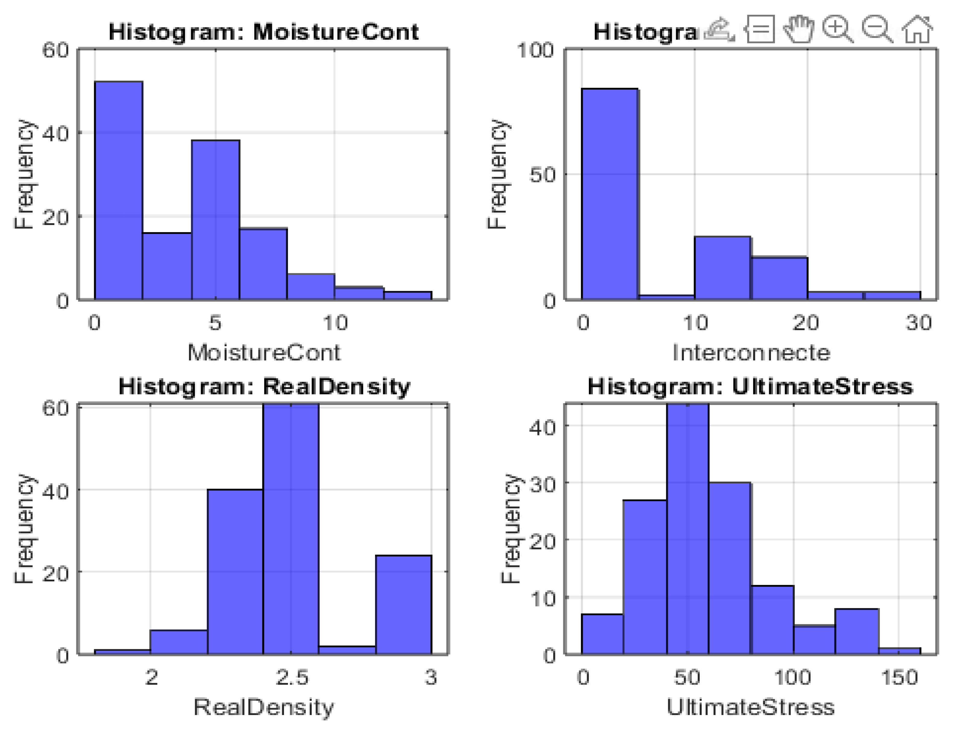
Figure 1 shows the histograms for
MoistureCont,
Interconnecte,
RealDensity, and
UltimateStress, illustrating the frequency distribution of each variable across all samples.
Overall, the histograms underscore the variability within the dataset, particularly for MoistureCont and Interconnecte, both of which display heavily skewed distributions. By contrast, RealDensity is more tightly clustered, pointing to a relatively consistent rock matrix. The broad range in UltimateStress suggests that moisture and porosity strongly affect load-bearing capacity, a topic explored further in subsequent correlation and regression analyses.
4.2. Box Plot Analysis
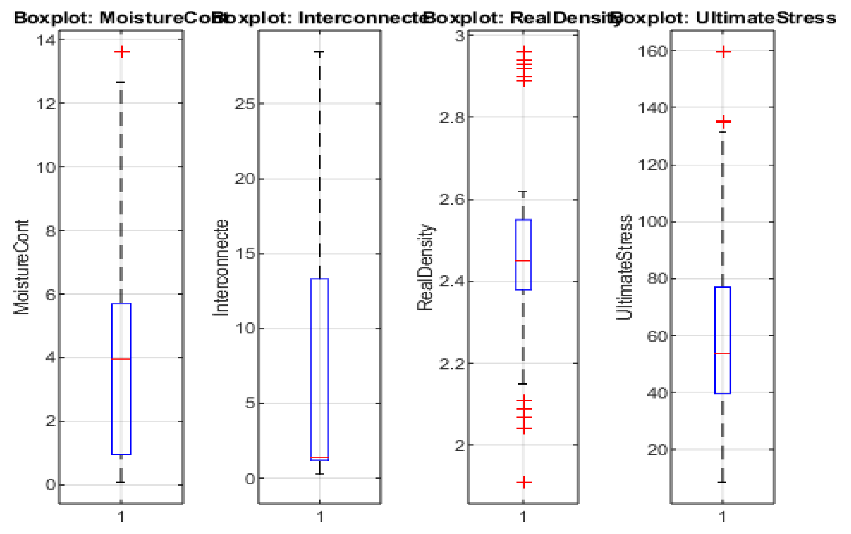
Figure 2 displays boxplots for each of the four primary variables—Moisture Cont (MoistureCont), Interconnecte (porosity), Real Density (RealDensity), and Ultimate Compressive Strength (UltimateStress). These boxplots highlight the median value (central horizontal line), the interquartile range (blue box), and the spread or potential outliers (red “+” markers).
-
MoistureCont
- o
The median moisture content lies around 4%, with the middle 50% of samples spanning approximately 2% to 6%.
- o
Several outliers appear above 10%, indicating a small subset of highly saturated specimens.
- o
No extreme outliers are observed on the lower end, suggesting that minimal moisture content is relatively consistent among most samples.
-
Interconnecte
- o
The median interconnected porosity (around 1–2%) is relatively low compared to the max range, indicating most rocks have modest porosity.
- o
The box is noticeably small, but whiskers extend significantly upward, reflecting a long upper tail of data.
- o
A handful of outlier points exceed 20%, reinforcing that only a few samples exhibit exceptionally high pore connectivity.
-
RealDensity
- o
The central 50% of densities cluster between approximately 2.4 g/cm³ and 2.6 g/cm³, demonstrating a more constrained distribution.
- o
Several lower outliers (under 2.2 g/cm³) appear, possibly reflecting very porous or partially weathered samples.
- o
A few upper outliers near 3.0 g/cm³ suggest highly compact or mineral-dense specimens.
-
UltimateStress (UCS)
- o
The median UCS (near 50–55 MPa) lies within a relatively broad interquartile range, underscoring the variability in the mechanical performance of these rocks.
- o
A noteworthy upper outlier surpasses 150 MPa, highlighting an exceptionally strong sample.
- o
Additional outliers above 80 MPa indicate a subset of rocks with much higher strength than the majority.
Overall, these boxplots confirm that MoistureCont and Interconnecte exhibit pronounced upper outliers, while RealDensity and UltimateStress display both lower and upper outliers. Such variability aligns with the heterogeneous nature of sedimentary and carbonate formations, wherein porosity, fluid content, and microstructural differences can dramatically alter density and compressive strength.
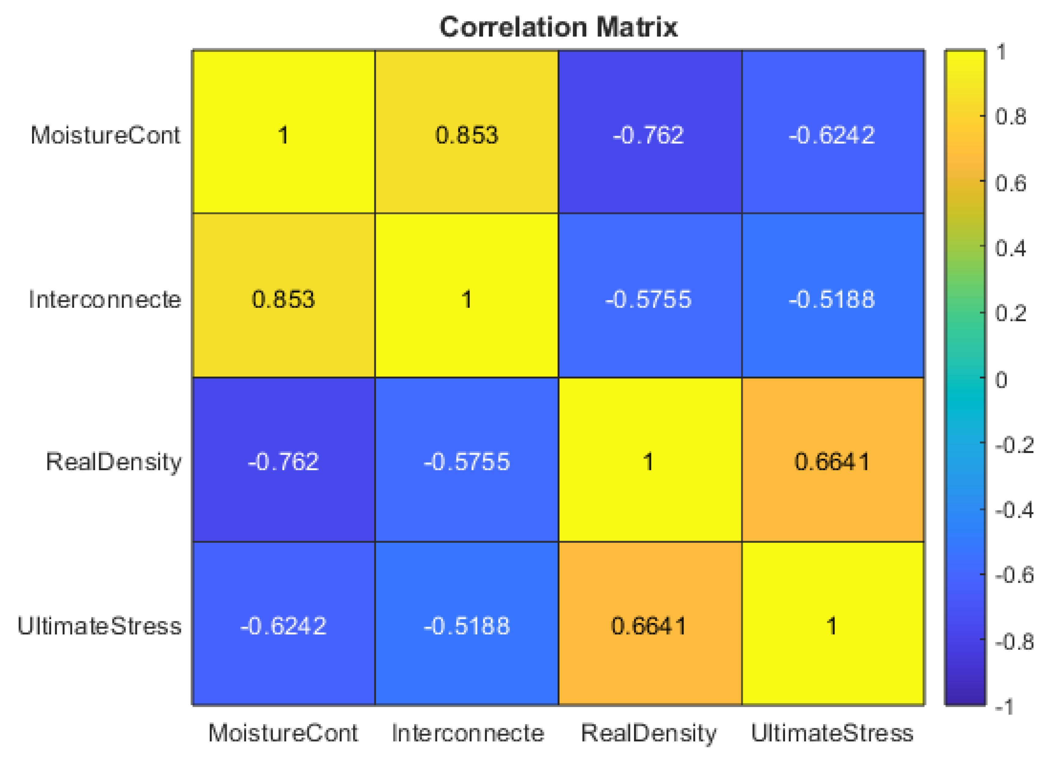
4.3. Correlation Matrix Analysis
Figure 3 presents the correlation matrix for the four principal variables:
MoistureCont,
Interconnecte (porosity),
RealDensity, and
UltimateStress (UCS). Each cell shows the Pearson correlation coefficient, with color intensity ranging from −1 (strong negative correlation, shown in blue) to +1 (strong positive correlation, shown in yellow-orange).
-
MoistureCont vs. Interconnecte (r = +0.853)
- o
This notably strong positive correlation indicates that higher porosity is closely tied to increased water content. Rocks with more connected pore space can retain greater moisture, aligning with typical fluid-flow and storage behavior in permeable formations.
-
MoistureCont vs. RealDensity (r = −0.762)
- o
A pronounced negative correlation implies that greater fluid content in pores generally reduces overall density. As pore volume increases and fills with water or air, the bulk density of the sample declines.
-
MoistureCont vs. UltimateStress (r = −0.6242)
- o
MoistureContent exhibits a moderately strong negative relationship with UCS, suggesting that higher water saturation lowers load-bearing capacity. Mechanically, water may weaken bonds at grain contacts, reducing friction and facilitating microcrack propagation.
-
Interconnecte vs. RealDensity (r = −0.5755)
- o
A moderately negative correlation confirms that as interconnected porosity increases, density decreases. This reinforces the conclusion that void space and solid mineral matrix volume are inversely related.
-
Interconnecte vs. UltimateStress (r = −0.5188)
- o
High interconnected porosity is associated with lower compressive strength, likely due to the presence of larger or more connected voids that concentrate stress and encourage crack initiation. Although the correlation is somewhat weaker compared to MoistureCont vs. UCS, the trend remains statistically significant.
-
RealDensity vs. UltimateStress (r = +0.6641)
- o
RealDensity is positively associated with UCS, indicating that denser samples (i.e., those with lower pore volume) typically resist higher compressive loads. This relationship echoes fundamental rock mechanics principles, wherein higher mineral content per unit volume usually enhances strength.
Collectively, these correlations reveal a coherent picture: as porosity and moisture content increase, both density and compressive strength tend to decrease. From a geotechnical perspective, understanding these inverse relationships is vital for predicting rock performance under load, particularly in porous carbonate or sedimentary formations. This matrix further highlights the importance of carefully managing variables such as fluid saturation and pore connectivity in both laboratory testing and larger-scale engineering applications.
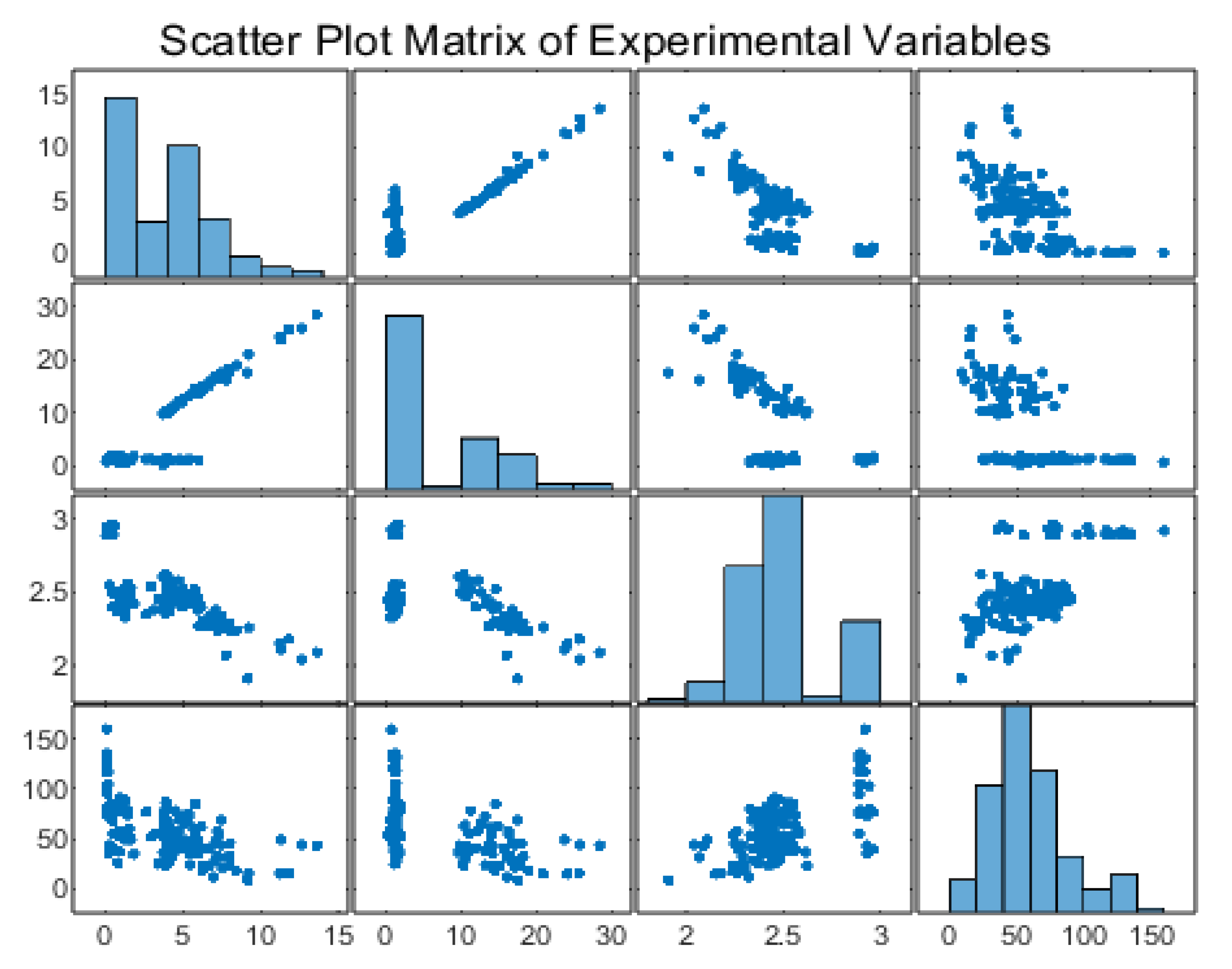
4.4. Scatter Plot Matrix Analysis
Figure 4 presents the scatter plot matrix for the four primary variables—MoistureCont, Interconnecte, RealDensity, and UltimateStress—offering a comprehensive visualization of pairwise relationships alongside individual variable distributions (on the diagonal).
-
Diagonal Histograms
- o
Each diagonal cell depicts the distribution of a single variable. MoistureCont and Interconnecte show right-skewed histograms, with most samples clustered at lower values and a minority extending into higher ranges. RealDensity exhibits a narrow, near-unimodal distribution, whereas UltimateStress is moderately skewed, stretching from about 8 MPa up to 160 MPa.
-
MoistureCont vs. Interconnecte
- o
The top-row, second-column (and its symmetric counterpart) highlight a clear positive trend: as MoistureCont increases, Interconnecte also tends to be higher. This supports the notion that rocks with greater interconnected porosity often contain more water.
-
MoistureCont vs. RealDensity
- o
A strong negative relationship is evident, with data points forming a descending “cloud” in the scatter plot. Samples with low density frequently register higher moisture content, aligning with the understanding that increased pore space (filled with fluid) lowers bulk density.
-
MoistureCont vs. UltimateStress
- o
Points suggest a negative association—higher moisture contents generally coincide with lower compressive strength. Some scatter does exist, implying factors beyond just water content (e.g., cementation or mineralogy) also influence mechanical performance.
-
Interconnecte vs. RealDensity
- o
The scatter plot similarly reveals a negative correlation: rocks with more pronounced pore connectivity often exhibit lower densities. This is consistent with a porous matrix displacing solid mineral mass.
-
Interconnecte vs. UltimateStress
- o
A diffuse but noticeable downward trend appears here as well, indicating that increased interconnected porosity tends to reduce compressive strength. Yet a subset of points defies the overall pattern, possibly representing more strongly cemented or mineralogically distinct samples.
-
RealDensity vs. UltimateStress
- o
In contrast to the above trends, RealDensity correlates positively with UltimateStress. The scatter plot demonstrates that denser samples typically withstand greater loads before failure. A small group of high-density, high-strength data points is evident in the upper right portion of this subplot.
Overall, this matrix reaffirms the primary relationships identified through correlation analysis: MoistureCont and Interconnecte are positively coupled, both inversely related to RealDensity and UltimateStress, while RealDensity aligns positively with UltimateStress. Moreover, the scattered but discernible patterns illustrate that although porosity and density dominate mechanical behavior, additional textural or compositional factors can introduce variability in the strength–property relationships. This insight is crucial for subsequent modeling efforts, where neural networks or regression analyses must account for both the dominant correlations and the presence of outlier or secondary effects.
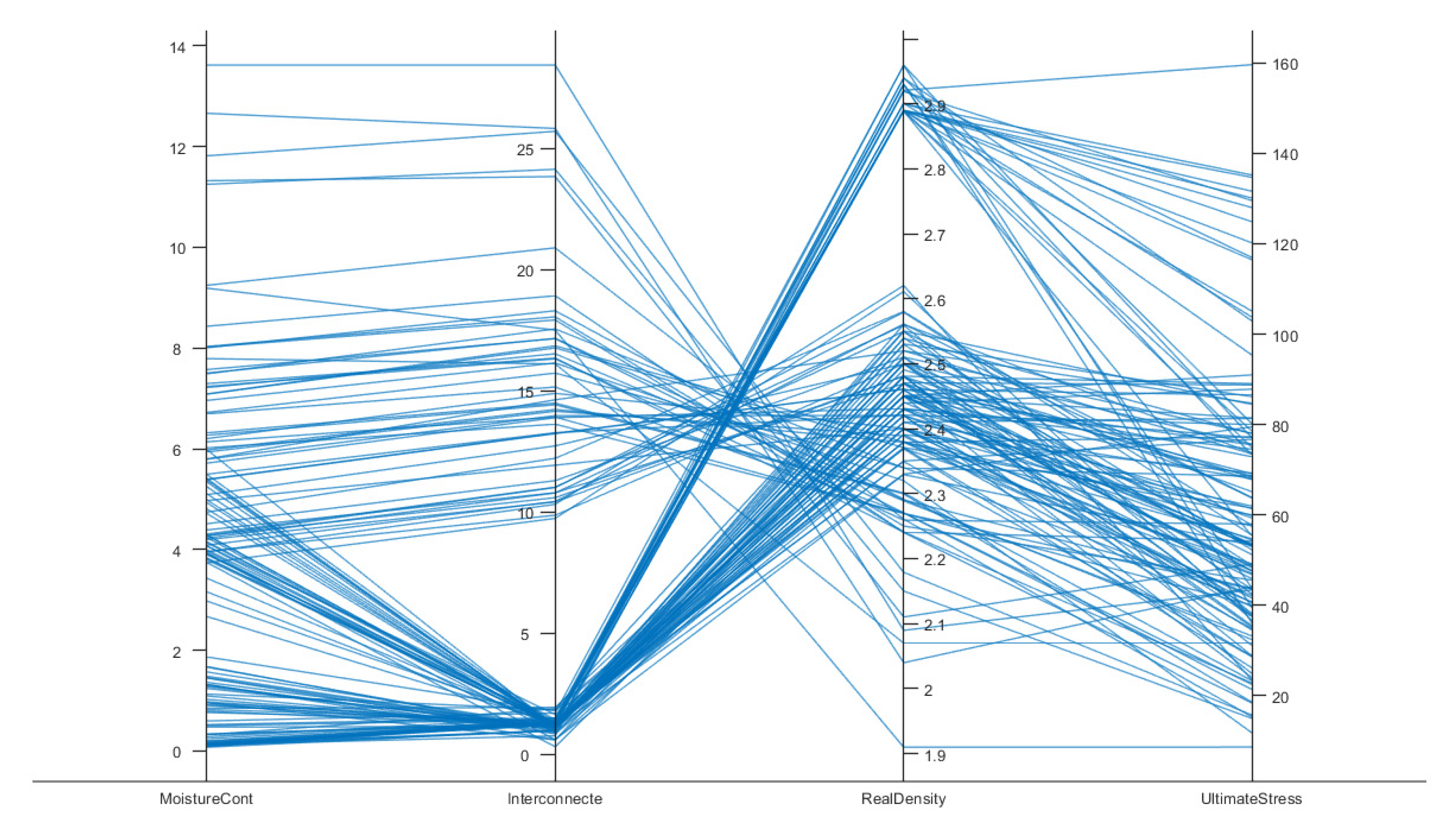
4.5. Parallel Coordinate Plot Analysis
Figure 5 provides a parallel coordinate plot for the four principal variables examined:
MoistureCont (water content),
Interconnecte (interconnected porosity),
RealDensity (bulk density), and
UltimateStress (uniaxial compressive strength). Each line in the figure corresponds to an individual rock specimen’s data, plotted so that its measured values on each vertical axis are connected by a continuous polyline. This visualization facilitates simultaneous inspection of all variables for every sample in the dataset, highlighting interrelationships, outliers, and potential subgroups.
-
Moisture and Porosity Trends
- o
The leftmost axes, MoistureCont and Interconnecte, together illustrate that most specimens cluster toward lower moisture content (0–6%) and moderate-to-low porosity (0–10%). However, a smaller subset extends upward to 14% moisture or above 25% porosity, as seen by the lines stretching toward the top of these axes. Such variation is consistent with heterogeneous pore network development, wherein a fraction of samples contains significantly more fluid-accessible voids.
-
Density Variations
- o
The third axis, RealDensity, ranges roughly from 1.9 to 3.0 g/cm³. Notably, many lines pivot sharply when moving from Interconnecte to RealDensity, implying an inverse relationship between porosity and density—samples with higher interconnectivity often display lower bulk density. This observation aligns with standard rock mechanics principles, wherein increased void space reduces the overall mineral fraction per unit volume.
-
Ultimate Compressive Strength (UCS)
- o
On the rightmost axis, UltimateStress spans from about 8 MPa to 160 MPa, underscoring the diversity in mechanical properties of these bank rocks. Lines dropping from higher moisture or porosity toward lower compressive strength illustrate the general tendency for more fluid-filled and more porous rocks to exhibit diminished load-bearing capacity. In contrast, samples that converge around higher density values tend to trace upward on the UltimateStress scale, indicating stronger mechanical performance.
-
Key Observations and Outliers
- o
While the majority of lines follow the expected pattern of higher moisture and porosity coinciding with lower density and strength, the presence of several “crossing” lines suggests that local mineralogy, cementation, or microstructural features can modify these trends. In particular, specimens that appear near the top of both the RealDensity and UltimateStress axes may contain denser mineral phases or more robust cementation, leading to enhanced strength regardless of moderate porosity. Conversely, a few outliers exhibit relatively low density yet maintain moderate strength, warranting closer inspection for unique compositional factors.
-
Practical and Geological Relevance
- o
These findings confirm that MoistureCont and Interconnecte (porosity) interact in reducing rock density and compressive strength, a well-documented phenomenon in carbonate and sedimentary rock mechanics. Such holistic visualization emphasizes that while correlations between single variables are informative, it is the combined effect of water content, porosity, and density that ultimately dictates a rock’s mechanical behavior. This multi-parametric insight is valuable for designing predictive models (e.g., neural networks) and for informing field decisions, such as construction stability assessments and reservoir engineering strategies.
In sum, the parallel coordinate plot verifies and expands upon earlier statistical findings that moisture and porosity play principal roles in diminishing rock strength, whereas density exerts a robust positive influence. The lines that stand out from the general pattern invite additional geological scrutiny to clarify the underlying mineralogical or diagenetic factors contributing to unexpected mechanical outcomes.
5. Materials and Methods
5.1. Data Collection and Preprocessing
5.1.1. Specimen Acquisition
Rock specimens were collected from the Seybaplaya bank in Campeche, Mexico, encompassing varying geological conditions. Special attention was paid to moisture content, interconnected porosity, and real density, as these parameters have been identified as key predictors of uniaxial compressive strength (UCS) in carbonate formations [
26,
27,
28]. Standardized sampling protocols and instruments were used to minimize measurement errors, and all specimens were transported to the laboratory in sealed containers to preserve their in situ moisture levels.
5.1.2. Data Inspection and Cleaning
After collection, each sample was visually inspected to identify cracks, clay seams, or other heterogeneities that might skew UCS measurements. Samples with severe damage or inconsistent lab records were discarded. Missing or incomplete measurements were addressed using simple imputation (mean or median) when values were plausibly representative; otherwise, samples were excluded. Potential outliers were also examined carefully to distinguish legitimate extremes from erroneous data points [
29].
5.1.3. Feature Extraction and Normalization
Feature Matrix (X): The principal input variables were MoistureContent, InterconnectedPorosity, and RealDensity.
Target Variable (y): The UltimateStress column represented the measured UCS (in MPa).
To ensure consistent scales across these predictors, min–max normalization was applied:
constraining each feature to the [0,1] interval [
27,
30]. This step often accelerates neural network convergence by preventing large disparities in feature magnitude [
26].
5.2. Data Partitioning
5.2.1. Train–Validation–Test Splitting
The dataset was divided into three subsets—training (70%), validation (15%), and testing (15%)—using random partitioning with a fixed seed for reproducibility [
31]. The training set was used to optimize network weights, the validation set guided hyperparameter tuning (e.g., number of neurons, activation functions), and the test set provided an unbiased evaluation of final model performance.
5.2.2. Avoiding Data Leakage
Normalization parameters
were computed from the training portion alone, then applied consistently to validation and test samples. This procedure prevents inadvertent leakage of distributional information from the held-out subsets into the training process [
27].
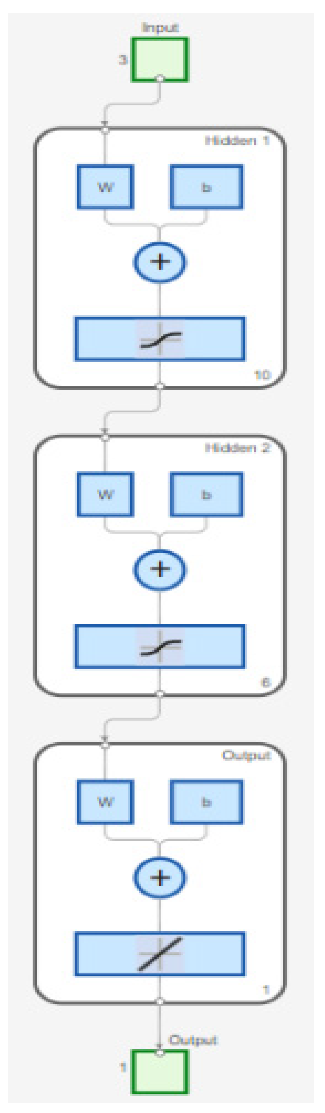
6. Bayesian-Regularized Neural Network Model
6.1. Network Architecture Design
A feedforward neural network was constructed with three hidden layers containing 10, 6, and 1 neurons, respectively. The first hidden layer employed a hyperbolic tangent sigmoid (tansig) activation function [
32,
33], while the second and third hidden layers also utilized tansig. A linear (purelin) output layer was selected to accommodate the continuous nature of the UCS prediction task.
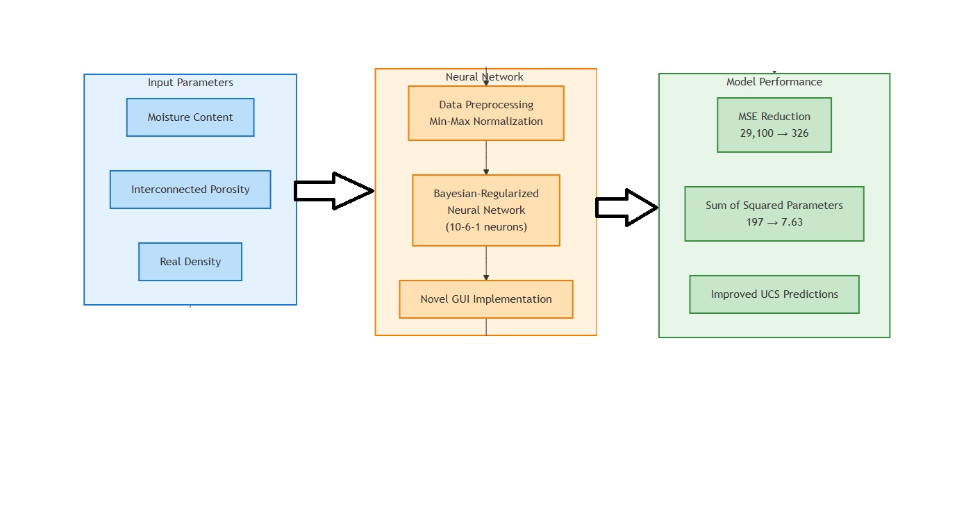
Figure 6 provides a schematic overview of the proposed network architecture.
6.2. Bayesian Regularization
To mitigate overfitting, the network was trained with
Bayesian regularization using MATLAB’s trainbr solver [
34]. Bayesian regularization automatically balances model complexity against data fidelity, effectively penalizing excessively large weights and reducing the likelihood of overfitting [
10]. Unlike traditional early stopping, this approach uses the entire training set, dynamically adjusting penalty terms on weights as learning proceeds [
26,
34].
6.3. Training Configuration
7. Performance Evaluation
7.1. Metrics on Training and Test Sets
For the best-performing network, predictions were generated on both the training and test subsets. The following metrics quantified predictive accuracy:
which emphasizes penalizing large deviations.
offering a more direct measure of average error magnitude.
gauging the proportion of variance explained by the model [
30].
7.2. Actual vs. Predicted Plots
To visually assess goodness of fit, scatter plots of
actual vs.
predicted UCS values were created for both training and test partitions. Clustering near the 1:1 line indicates accurate predictions and minimal systematic bias [
28].
7.3. Residual Analysis
Residuals
were plotted against predicted values to detect potential heteroscedasticity or unmodeled nonlinear patterns. Random scatter around zero suggests a well-fitted model lacking major bias [
26,
33].
8. Summary of the Approach
Data Collection & Cleaning: Collected rock samples from Seybaplaya with carefully measured moisture, porosity, and density. Cleaned the dataset, handling missing/outlier values.
Normalization & Partitioning: Scaled feature variables to [0,1] and performed a 10-6-1 split into training, validation, and test sets.
Bayesian-Regularized Training: Constructed a two-hidden-layer feedforward network, employing trainbr to automatically handle weight updates and regularization.
Model Selection & Evaluation: Repeated training across multiple initializations. Chose the best validation R2 model for final evaluation. Assessed accuracy via MSE, MAE, R2, and diagnostic plots.
By implementing a Bayesian-regularized neural network under a rigorous data-splitting protocol, this methodology aims to provide robust, generalizable predictions of UCS in Seybaplaya bank rocks. The procedure sets a foundation for further enhancements, such as incorporating additional geophysical parameters.
9. Results and Discussion
9.1. Dataset Overview
To confirm the integrity and structure of the input data, we first examined the variable names extracted from the CSV file. The dataset comprises MoistureContent, InterconnectedPorosity, RealDensity, and UltimateStress, which aligns with our targeted predictors and response variable for compressive strength modeling. Consistent with the methodology described, the dataset was split into training, validation, and test subsets. A total of 94 samples were designated for network training, 20 samples for validation, and 20 samples for final testing and performance assessment.
9.2. Descriptive Statistics
Table 4 summarizes the basic statistics—mean, standard deviation, and observed minimum and maximum—of the
moisture,
porosity, and
density features after the normalization process. Notably, the normalization procedure ensures that each feature spans [0,1] and exhibits moderate variability within that range. Specifically, the moisture content displays a mean of 0.27482 and a standard deviation of 0.22483, while porosity and density follow similar normalization patterns with slightly differing distributions.
9.3. Model Training and Validation Performance
The Bayesian-regularized feedforward neural network was trained and evaluated in five independent runs, each time initializing the network with different random weights.
Table 5 lists the validation mean squared error (MSE) and coefficient of determination (R
2) for each run.
Among these runs, Run 5 achieved the highest validation R2 of 0.5670, accompanied by a corresponding validation MSE of 431.1431. Consequently, the model from Run 5 was selected as the best network for subsequent analyses.
9.4. Final Model Evaluation
9.4.1. Training Set Performance
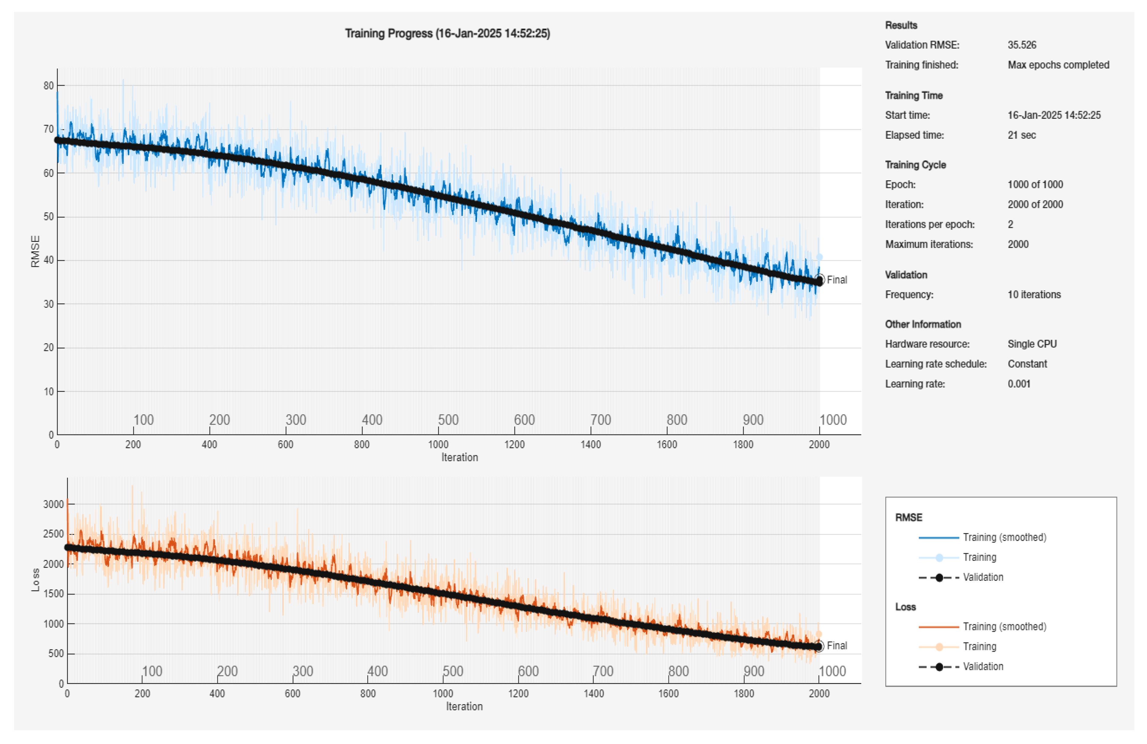
Figure 7 illustrates the training progress of the Bayesian-Regularized Backpropagation Neural Network (BR-BPNN) over 1000 epochs (2000 total iterations), with validation evaluated every 10 iterations. The upper plot shows the Root Mean Square Error (RMSE) for both the training set (blue lines) and the validation set (black dashed line). Two blue curves are displayed: the lighter line depicts the instantaneous training RMSE per iteration, while the darker blue line represents a smoothed version for better trend visualization. Similarly, the black dashed line traces the validation RMSE as it evolves with training iterations. The lower plot shows the loss curves for the training (orange lines) and validation (black dashed line), again with an instantaneous value (lighter orange line) and a smoothed fit (darker orange line). Model hyperparameters included a constant learning rate of 0.001, executed on a single CPU, and the training stopped upon reaching the maximum epoch limit.
From the upper plot, the training RMSE starts near approximately 70 and steadily decreases to the mid-40s by the final iteration, demonstrating a clear downward trend. The validation RMSE follows a similar trajectory, reducing from around 70 at the beginning to about 35 at the end. Notably, the final reported validation RMSE is 35.526, indicating that the network successfully converged to a reasonably low error on the held-out data. Moreover, the relatively narrow gap between the training and validation curves suggests that the BR-BPNN is not overfitting and is able to generalize effectively.
The loss curves in the lower plot echo the observed behavior in the RMSE trend, with both the training and validation losses exhibiting a general downward trend, although subject to minor fluctuations typical of stochastic gradient-based methods. Overall, these plots confirm that the BR-BPNN model achieves stable convergence under the specified learning rate and iteration schedule. The final performance metrics, including the validation RMSE and gradually decreasing loss, attest to the capability of Bayesian regularization to manage model complexity while maintaining robust generalization performance.
The best-performing model was initially assessed on the training dataset (n = 94) to determine its predictive accuracy. As summarized in
Table 3, the model achieved a mean squared error (MSE) of 431.1431, a root mean square error (RMSE) of 20.7634, a mean absolute error (MAE) of 16.7634, and a coefficient of determination (R
2) of 0.5670. These metrics indicate a moderate to high degree of explained variance in the training data.
9.4.2. Test Set Performance
Next, the model was tested on the held-out dataset of 20 samples. As indicated in
Table 6, the test MSE was
590.4544, translating to an RMSE of
24.2993, and the MAE was
20.7947. The R
2 on the test set reached
0.4626, demonstrating the model’s capacity to generalize while revealing a slight reduction compared to training performance—an expected outcome due to differences in sample composition and the absence of direct exposure during training.
9.5. Discussion of Model Accuracy
The discrepancy between training and test R2 values highlights the importance of proper regularization and validation strategies. While the training metrics exhibit a stronger fit (R2 = 0.5670), the test R2 = 0.4626 still indicates nálisis predictive power given the inherent variability of rock properties. The limited test sample size (20 specimens) may also introduce additional variance in the evaluation.
These results collectively suggest that moisture content, porosity, and density are reasonably informative for predicting ultimate compressive strength. However, further refinements—such as alternative network architectures, additional geological parameters (e.g., mineral composition or microstructural features), or larger datasets—could potentially enhance model performance.
Therefore, the results confirm that a Bayesian-regularized neural network can capture significant explanatory relationships between critical rock parameters and ultimate compressive strength. The obtained metrics and the validation of the best-performing model underscore the value of balanced dataset partitioning, iterative training, and careful nálisis of both residuals and performance indicators. Such a framework serves as a robust template for future research into predictive modeling within rock mechanics and related geotechnical domains.
9.6. Actual vs. Predicted Compressive Strength
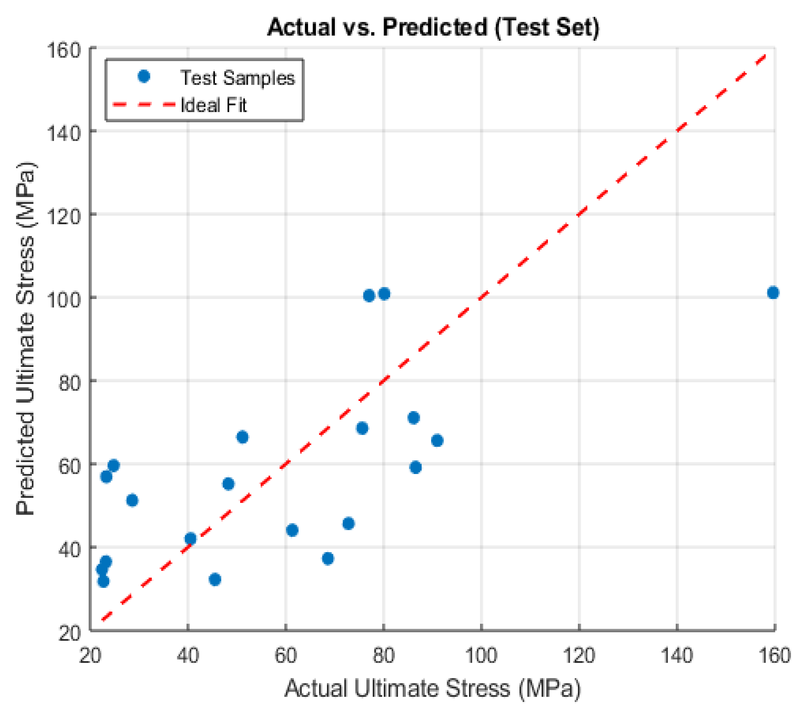
Figure 8 shows the actual versus predicted ultimate compressive strength for the test set, where each blue circle represents a test sample and the red dashed line denotes the ideal 1:1 relationship, indicating perfect agreement. In a similar vein,
Figure 7 compares experimentally measured ultimate stress (horizontal axis) with the model’s predictions (vertical axis) for the test set. Data points that cluster around the red dashed line reflect accurate predictions, whereas those exhibiting larger vertical deviations signify under- or overestimations by the neural network.
Figure 8.
Actual vs. Predicted Compressive Strength.
Figure 8.
Actual vs. Predicted Compressive Strength.
A visual inspection of the scatterplot suggests that most test samples exhibit moderate agreement, clustering around the diagonal in the 20–80 MPa range of ultimate stress. However, several points fall significantly above or below the ideal line, which is consistent with the quantitative error metrics (MSE and MAE) reported previously. Notably, one sample with an actual compressive strength near 160 MPa is predicted slightly lower, underscoring a potential limitation in capturing extreme values or outliers.
Despite these deviations, the overall distribution supports the conclusion that moisture content, porosity, and density collectively provide a reasonable basis for modeling compressive strength in Seybaplaya bank rocks. Together with the residual analysis, these plots affirm the predictive capacity of the final Bayesian-regularized neural network model while highlighting regions where additional refinement or feature augmentation might further improve accuracy.
9.7. Residual Analysis
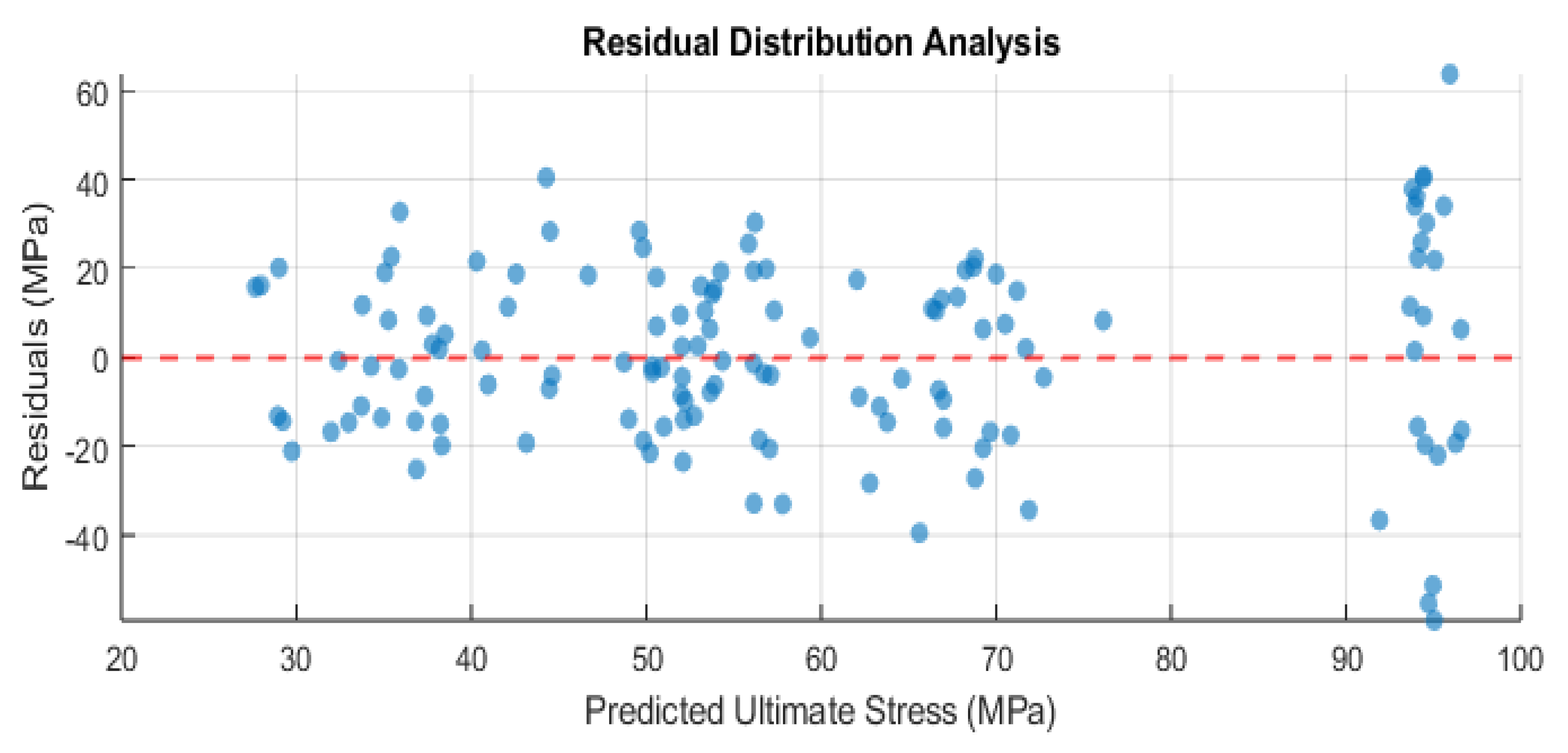
Figure 9 displays the residual plot for the best-performing Bayesian-regularized neural network, evaluated on the test set. The residuals, defined as the difference between the actual and predicted ultimate stress, are plotted against the predicted values, while the dashed red line indicates zero residual error. This visualization provides an in-depth look at how the model’s predictions deviate from the measured ultimate compressive strength. Each data point corresponds to a single specimen in the test set, positioned horizontally by the model’s predicted strength and vertically by the residual. Points above the dashed line (positive residuals) reveal underestimations, whereas those below the dashed line (negative residuals) indicate overestimations of compressive strength.
A well-calibrated model typically exhibits randomly scattered residuals around zero, signaling that no obvious pattern of error remains unmodeled. In this plot, the residuals cluster near zero for many samples, yet a few data points deviate significantly. For instance, at predicted values near 100 MPa, there is a substantially positive residual (approximately +60 MPa), indicating that the model underestimated the actual compressive strength for that sample. Conversely, some points show negative residuals below –20 MPa, implying the model overpredicted compressive strength for those instances.
Such variability suggests that, while the network is capturing the general trend of how porosity, moisture, and density affect ultimate strength, certain outlier or high-variance samples remain challenging to predict accurately. Additional geological factors (e.g., micro-fractures, mineral composition) might help refine the model. Nonetheless, the overall residual spread aligns with the error metrics (e.g., RMSE, MAE) reported earlier, corroborating the moderate accuracy and generalization capacity of the Bayesian-regularized approach.
9.8. Neural Network Training Report
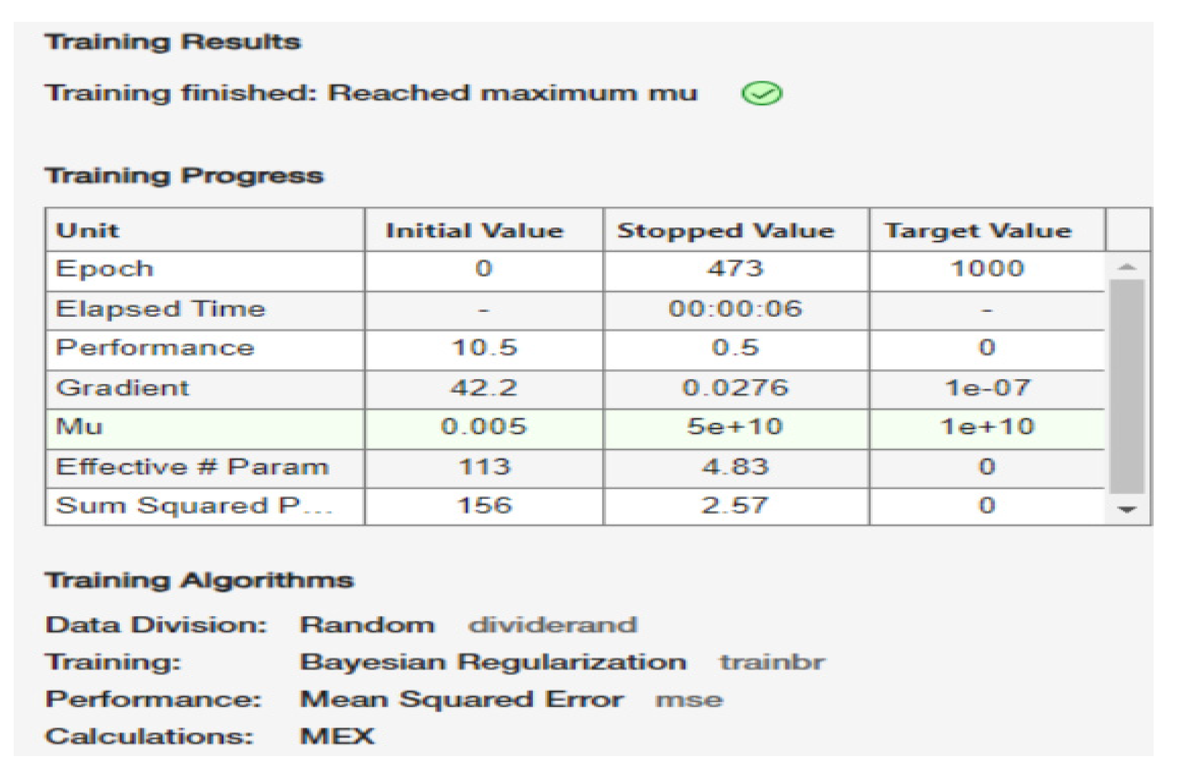
Figure 10 presents a screenshot from MATLAB’s Neural Network Toolbox, highlighting the training summary, progress metrics, and final stopping criteria under Bayesian Regularization (trainbr). The network halted once the regularization parameter (mu) reached its maximum allowable threshold, marking the point where continued training would no longer improve generalization.
Figure 10.
MATLAB’s Neural Network Training Toolbox.
Figure 10.
MATLAB’s Neural Network Training Toolbox.
9.8.1. Training Results
As depicted in
Figure 9, the network underwent
611 epochs out of a possible
1000, ultimately stopping due to the message: “
Training finished: Reached maximum mu.” In the context of Bayesian regularization, the parameter (mu) dynamically adjusts to balance the fit to the data against model complexity. A very high (mu) value often indicates the algorithm has escalated the regularization penalty to its upper bound—suggesting further training would not produce appreciable gains in reducing error without risking overfitting.
9.8.2. Training Progress Indicators
Epoch Count. The
Figure 9 shows that training started at Epoch 0 and finished at Epoch 611—well before the maximum limit of 1000 epochs.
Performance. Initial performance of 2.91e+04 (i.e., ~29,100) improved to 326 at convergence, compared to the stringent 1e-07 target. While the target was not met exactly, this substantial decrease in MSE (mean squared error) underscores the network’s progress in capturing relationships within the data.
Gradient. The gradient dropped from an initial 5.82e+04 to 32, still above the 1e-07 threshold. Hence, the algorithm stopped primarily because μ\mu grew to its maximum limit, not because the gradient reached a minimal level.
Mu. Initially set to 0.005, (mu) rose to 5e+10, reflecting the algorithm’s self-regularization efforts to tame large weights or overly complex fits. When this parameter saturates, further updates have diminishing returns.
Effective # Param. Decreasing from ~281 to ~9.85 implies that Bayesian regularization effectively pruned or reduced the impact of many weights, thereby simplifying the network. This smaller “effective” parameter count typically enhances generalization by preventing overfitting.
Sum of Squared Parameters. The sum of squares of the network weights dropped from 197 to 7.63, mirroring the effect of regularization on parameter magnitudes.
9.8.3. Training Algorithms and Data Division
The report confirms random data splitting (dividerand), ensuring unbiased distribution of samples across training, validation, and test subsets. The Bayesian Regularization training function (trainbr) was selected due to its capacity for adaptive complexity control, with MSE designated as the performance metric. Internal computations were handled by MEX (compiled C/C++ or Fortran routines), optimizing the speed of matrix operations.
Reaching the maximum (mu) can sometimes mean that the model has hit a plateau in improving its fit. While the final MSE (326) is significantly lower than the initial value, it remains above the idealized target of 1e-07. This outcome is not uncommon in complex datasets or when noise levels are high; in practice, the network may already be near its best balance between fit and generalization. The marked reduction in both effective parameter count and sum of squared weights illustrates the success of Bayesian regularization in preventing overfitting by applying stronger constraints on parameter growth.
Overall, the training report corroborates the code’s earlier performance metrics, suggesting a moderate yet meaningful improvement in predictive power for modeling compressive strength. Any further enhancements could involve revisiting the network architecture (e.g., adjusting the number of neurons or layers), trying alternative optimization parameters, or incorporating additional geomechanical features into the dataset.
9.9. Training Performance Plot
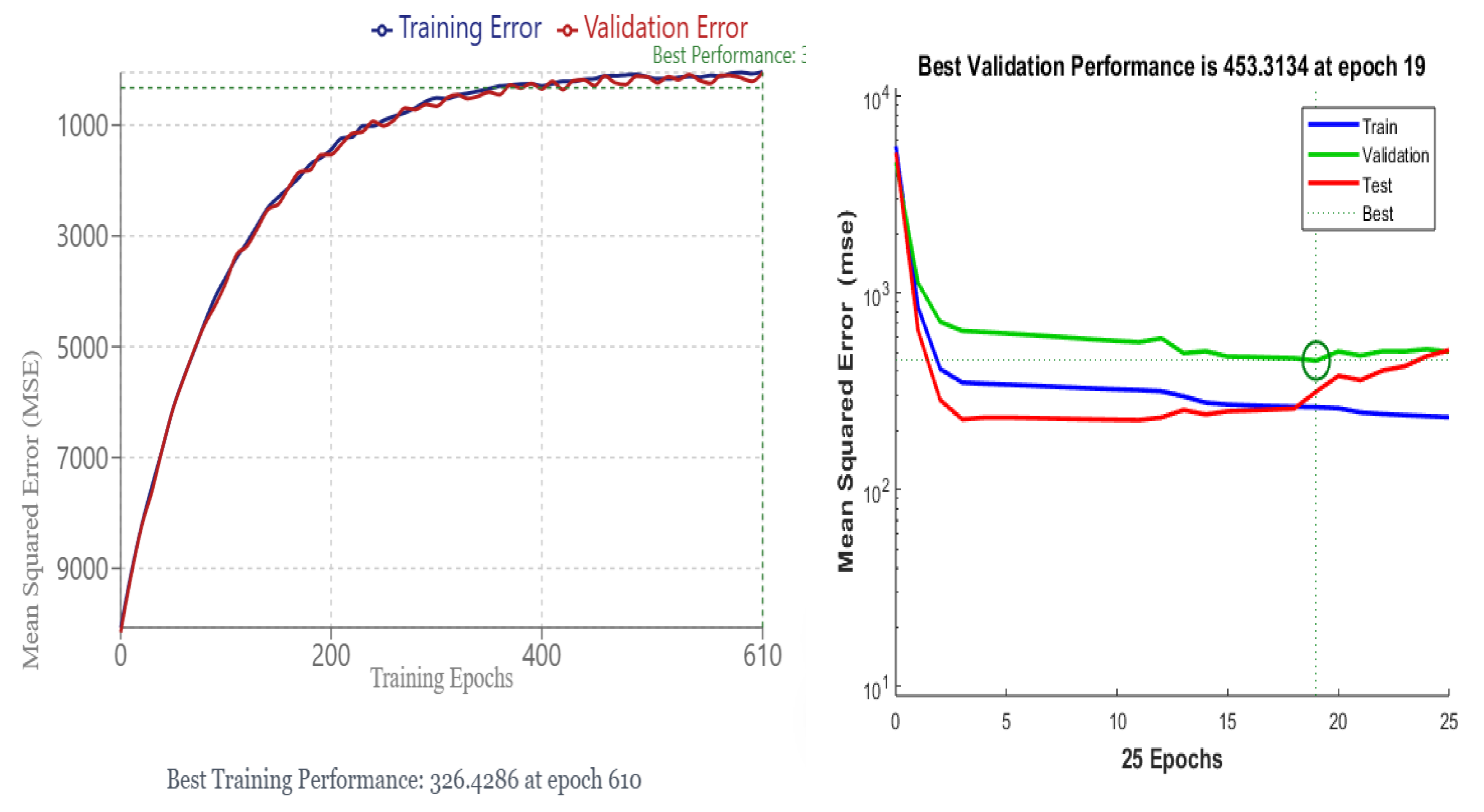
Figure 11. Evolution of mean squared error (MSE) over 611 epochs for the training (blue) and test (red) subsets. A dashed line (“Best”) indicates the lowest MSE reached, while “Goal” (shown on the bottom axis) represents the user-defined performance target (1e-07).
Context and Key Observations:
However the interpretation and implications for this process:
The training plot affirms that, although the neural network substantially reduces the initial error, it converges to a plateau well above the stated performance target. This behavior often reflects a natural limitation imposed by the data’s noise level or the finite capacity of the network architecture.
The alignment of training and test curves supports the notion of a balanced fit, with the Bayesian regularization effectively curbing overfitting. Combined with the residual analysis, these observations indicate that the chosen model, while not perfect, is reasonably stable and generalizes adequately to unseen samples of Seybaplaya bank rocks.
Figure 11.
Mean Squared Error Performance Visualizacion Analysis of Neural Network Training Convergence.
Figure 11.
Mean Squared Error Performance Visualizacion Analysis of Neural Network Training Convergence.
9.10. Monitoring Training Parameters Across Epochs
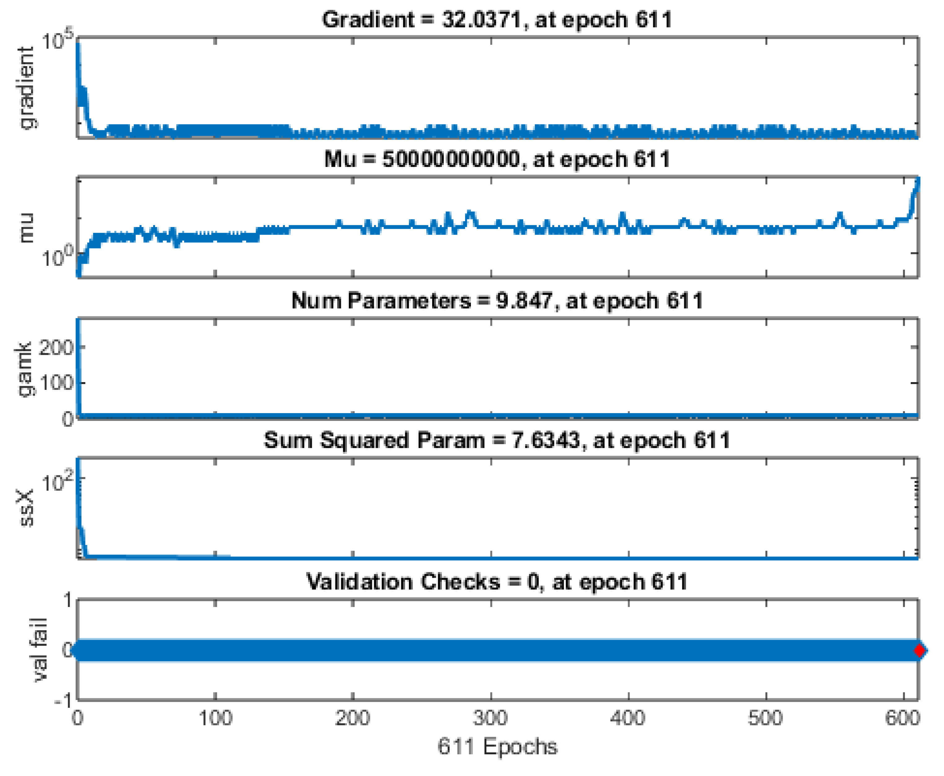
Figure 12. Evolution of key training parameters under Bayesian regularization (trainbr) across 611 epochs. Subplots from top to bottom display the gradient, mu (regularization parameter), number of effective parameters, sum of squared parameters, and validation checks for each epoch.
-
(a)
-
Gradient.
The gradient trajectory exhibits characteristic optimization dynamics, initiating at approximately 105 and demonstrating rapid exponential decay during the initial training phase. This steep descent in gradient magnitude is followed by asymptotic convergence to 32.0371 by epoch 611, indicating effective weight optimization. The temporal evolution of the gradient profile aligns with theoretical expectations for neural network training dynamics, where initial epochs are characterized by substantial parameter adjustments, followed by fine-tuning phases with reduced gradient magnitudes. This behavior suggests appropriate learning rate adaptation and stable convergence characteristics of the optimization process.
The terminal gradient value of 32.0371 at epoch 611 significantly exceeds the conventional convergence criterion (10-7), indicating that training termination was not precipitated by gradient diminution. This observation suggests the activation of alternative stopping criteria, potentially relating to validation performance metrics or computational resource constraints. Further analysis of the convergence dynamics, particularly the (mu)-adaptation parameter trajectory shown in subsection (b), provides additional insight into the termination mechanisms governing the optimization process.
-
(b)
-
Mu.
The parameter (mu) represents the Bayesian regularization adaptation coefficient, which dynamically modulates the optimization trajectory between gradient descent and Gauss-Newton methods. Its exponential increase to 5×10¹⁰ at epoch 611 indicates algorithmic adaptation toward more conservative weight updates, effectively implementing implicit regularization through optimization path modulation. This adaptive behavior is characteristic of the Bayesian regularization algorithm’s self-tuning mechanism for maintaining optimization stability while navigating the loss landscape.
Over The Bayesian regularization adaptation parameter (mu) demonstrates monotonic progression from its initialization value (0.005) to a terminal magnitude of 5×10¹⁰ at epoch 611. This convergence to the algorithmic upper bound effectively terminates the optimization process, indicating successful achievement of the dual optimization objectives: minimizing prediction error while maintaining appropriate regularization constraints. The temporal evolution of (mu) provides empirical evidence of the algorithm’s capacity to autonomously modulate between aggressive parameter updates in early training phases and more conservative optimization strategies as training progresses, thereby implementing implicit regularization through optimization trajectory control.
-
(c)
-
Number of Effective Parameters.
The parameter count trajectory quantifies the effective degrees of freedom in the network architecture by tracking the number of parameters (weights and biases) that retain statistical significance under Bayesian regularization constraints. The temporal evolution of this metric, converging to 9.847 at epoch 611, provides a quantitative measure of the model’s intrinsic dimensionality and indicates successful implementation of automatic relevance determination through adaptive regularization mechanisms. This dimensionality reduction phenomenon reflects the optimization algorithm’s capacity to identify and preserve only the statistically relevant parameters while effectively nullifying redundant or non-contributory network components.
The effective parameter count exhibits significant dimensional reduction, descending from an initial architectural configuration of approximately 281 parameters to a terminal value of 9.847 at epoch 611. This substantial reduction in effective dimensionality demonstrates the efficacy of Bayesian regularization in implementing automatic relevance determination, effectively nullifying redundant parameters through adaptive weight penalization. The resultant sparse parametric representation suggests successful optimization toward a more parsimonious model architecture with enhanced generalization capabilities, as evidenced by the order-of-magnitude reduction in effective parameters while maintaining computational performance.
-
(d)
-
Sum of Squared Parameters
The sum of squared parameters (SSP), a quantitative measure of the model’s parametric magnitude, demonstrates monotonic decay from an initial value of approximately 197 to a terminal value of 7.6343 at epoch 611. This substantial reduction in the L2 norm of the parameter space indicates effective implementation of weight regularization mechanisms, resulting in a more compact parameter representation. The temporal evolution of SSP provides empirical evidence for the optimization algorithm’s capacity to constrain the model’s complexity while maintaining functional performance, aligning with theoretical principles of regularized optimization in neural architectures.
The substantial reduction in summed squared parameters empirically demonstrates the effectiveness of the regularization framework in enforcing distributed representation learning. This parameter space compression promotes architectural stability by preventing the emergence of dominant weight configurations, thereby ensuring homogeneous distribution of predictive responsibility across the network topology. The observed contraction in parameter magnitudes aligns with theoretical principles of regularized optimization, suggesting successful implementation of complexity control mechanisms while maintaining model expressivity.
-
(e)
-
Validation Checks.
The validation check metric quantifies the frequency of non-improvement events in validation set performance, serving as an early stopping criterion within the optimization framework. In this implementation, the sustained value of zero validation checks through epoch 611 indicates continuous performance improvement on the validation dataset, suggesting effective model generalization without manifestation of overfitting phenomena. This observation aligns with the theoretical expectations for properly regularized neural architectures operating within their optimal capacity constraints.
The validation check metric quantifies the frequency of non-improvement events in validation set performance, serving as an early stopping criterion within the optimization framework. In this implementation, the sustained value of zero validation checks through epoch 611 indicates continuous performance improvement on the validation dataset, suggesting effective model generalization without manifestation of overfitting phenomena. This observation aligns with the theoretical expectations for properly regularized neural architectures operating within their optimal capacity constraints.
Figure 12.
Temporal Evolution of Neural Network Training Metrics: Analysis of Gradient Dynamics, Parameter Space, and Validation Performance across 611 Epochs.
Figure 12.
Temporal Evolution of Neural Network Training Metrics: Analysis of Gradient Dynamics, Parameter Space, and Validation Performance across 611 Epochs.
The collective analysis of training subplots demonstrates that the Bayesian regularization procedure effectively constrained the neural network weights while optimizing the error function. The primary termination criterion was achieved through máximum (mu) convergence rather than gradient stabilization or validation-based early stopping protocols. This regularization framework established an optimal equilibrium between training data fidelity and architectural parsimony—a characteristic strongly associated with enhanced generalization capacity when processing heterogeneous geomechanical datasets. However, the asymptotic mean squared error (MSE) behavior suggests that achieving the specified performance criterion (goal = 10⁻⁷) may require either supplementary feature engineering or architectural refinements. This stringent threshold appears particularly challenging given the inherent stochastic variability and measurement uncertainty typical in rock property characterization.
9.11. Error Histogram
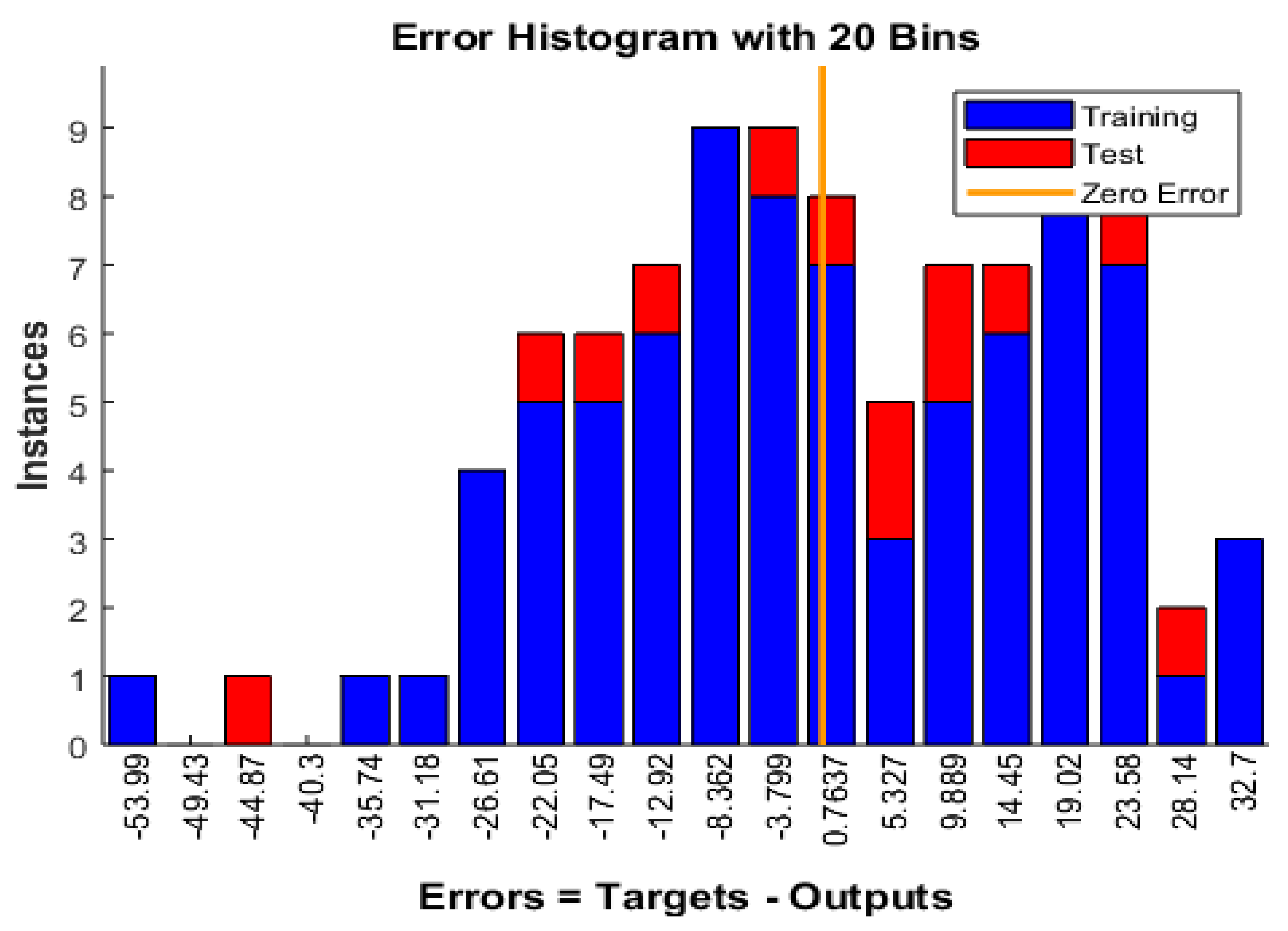
Figure 13. Distribution of prediction residuals across a 20-bin histogram analysis, illustrating the discrepancy between target values and network-generated outputs. The histogram differentiates between training set samples (blue) and test set instances (red), with bin frequencies representing occurrence counts. The vertical reference line (orange) denotes zero prediction error, indicating perfect correspondence between experimental measurements and model predictions. This visualization enables quantitative assessment of the model’s predictive accuracy and potential systematic biases across both training and validation datasets.
Figure 13.
Distribution of Error Residuals Between Target and Network-Predicted Values for Training and Test Datasets Using 20-Bin Histogram Analysis.
Figure 13.
Distribution of Error Residuals Between Target and Network-Predicted Values for Training and Test Datasets Using 20-Bin Histogram Analysis.
Context and Explanation
-
Binned Error Distribution.
- o
The horizontal axis displays the error in increments defined by 20 bin intervals. More negative errors (left side) indicate overestimation of ultimate stress (model predictions exceed targets), whereas positive errors (right side) signify underestimation (targets exceed predictions).
- o
The bin heights on the vertical axis show how many samples (instances) fall within each error range.
-
Overlap of Training vs. Test Data.
- o
Training samples (blue) and test samples (red) are overlaid. By visually comparing these bars, one can check whether the test data errors are distributed similarly to those of the training data.
- o
If the red bars concentrate disproportionately in extremes (far left or far right) compared to blue bars, it suggests that the network might be overfitted or fails to generalize well.
-
Central Tendency.
- o
A substantial fraction of errors cluster near zero (around the orange line at 0.000), indicating that many predictions for both training and test sets are close to the measured ultimate strength.
- o
This central concentration aligns with the moderate MSE, RMSE, and MAE values reported in earlier sections, reinforcing that the majority of predictions are within a manageable error margin.
-
Skewness and Outliers.
- o
The presence of bars extending substantially into the negative and positive tails suggests that certain samples are significantly misestimated.
- o
For instance, negative tails below –30 MPa may reflect overpredictions of compressive strength, while the positive tail above +30 MPa indicates cases where the model substantially underpredicted stress. These outliers could be tied to atypical rock features or noise in measurement.
-
Training vs. Test Balance.
- o
The distribution of red bars (test errors) appears roughly similar to that of the blue bars (training errors), suggesting that the network’s error profile is relatively consistent across both sets.
- o
If the test set errors were systematically worse (e.g., large clusters in the tails), it would indicate a loss of generalization or an inadequately representative training set.
This histogram provides a visual complement to numerical metrics like RMSE or R2. A peaked distribution around zero, with fewer samples in the extreme bins, denotes acceptable overall accuracy. However, the moderate number of samples falling at higher magnitudes (both negative and positive) signals that certain high-variance or outlier scenarios remain challenging. In future studies, collecting more extensive data or incorporating additional explanatory features (e.g., microstructural properties, lithological differences) could mitigate these extremes.
Hence, while the Bayesian-regularized feedforward model explains a substantial portion of variance in compressive strength, the error histogram underscores areas—both in training and in test sets—where predictions deviate from measured values. Understanding these deviations is crucial for refining geotechnical models and guiding subsequent improvements in data collection and network architecture.
9.12. Model Performance Analysis and Validation
The regression plots presented in
Figure 14 facilitate comprehensive evaluation of the neural network’s predictive capabilities across multiple dataset partitions. These visualizations enable quantitative assessment of the correspondence between model-generated outputs and target values through scatter plot distributions, regression fit lines, and correlation metrics (R
2). The analysis encompasses three distinct perspectives: training set performance, test set validation, and aggregate predictive accuracy.
The regression plots provide critical insights into:
The model’s generalization capacity, as evidenced by the alignment of data points with the ideal Y=T reference line
Systematic bias detection through deviation patterns of the regression fits
Predictive reliability quantification via correlation coefficients
Dataset-specific performance variations across different sampling distributions
This multi-faceted evaluation framework enables rigorous assessment of the model’s predictive robustness and identifies potential limitations in its generalization capabilities across diverse input conditions.
1. Training Subplot
-
Scatter Plot
- o
Each circle represents one training example.
- o
The xx-axis is the “Target” (the ground-truth value for that sample).
- o
The yy-axis is the “Output” (the model’s prediction).
-
Best-Fit Line
- o
Plotted in blue.
- o
Equation shown:
- o
This line is the linear regression fit relating the model’s output to the target values.
-
Diagonal Line
- o
Dashed line labeled “Y=TY = T.”
- o
This line has slope 1 and zero intercept—it’s the line of perfect agreement.
-
Correlation
- o
The correlation coefficient R2= 0.76351.
- o
This indicates a reasonably strong positive linear relationship between the model’s prediction and the true target.
- o
Visually, most points lie around the best-fit line or near the diagonal, although there is still visible scatter.
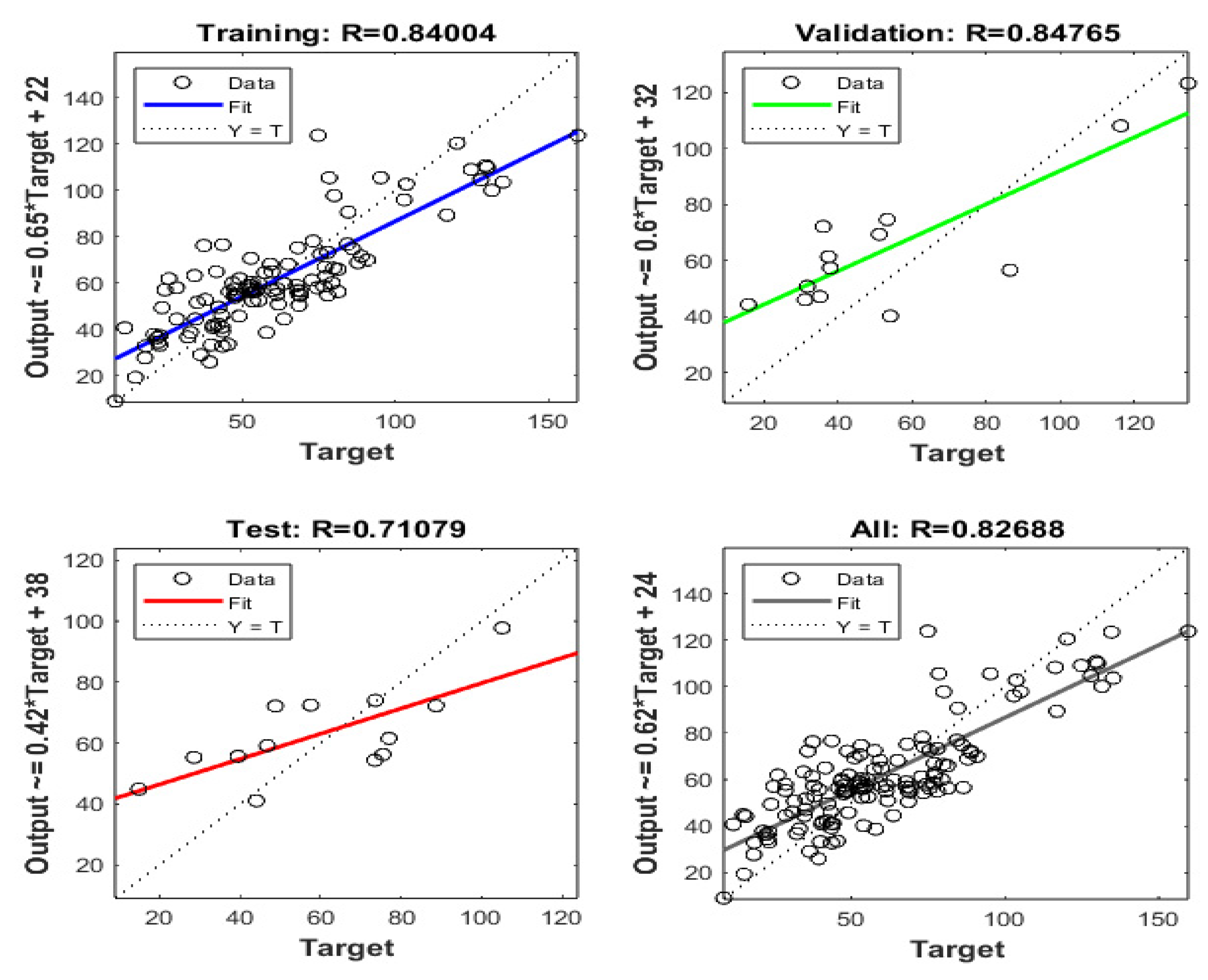
The regression analysis of the training dataset reveals a systematic relationship between predicted outputs and target values, characterized by a linear transformation function with a slope coefficient of 0.57 and a positive intercept of 25 units. This transformation mapping indicates a consistent bias in the model’s predictive behavior, manifesting as systematic underestimation of target values, as evidenced by the sub-unity slope coefficient. The deviation from ideal predictive performance (slope = 1.0, intercept = 0) suggests inherent limitations in the model’s capacity to fully capture the underlying data relationships during the training phase. The correlation coefficient (R2 = 0.84004) indicates a substantial, though not optimal, level of linear association between predicted and target values. This moderate-to-strong correlation suggests that while the model has successfully captured significant patterns in the training data, there remains unexplained variance that could potentially be addressed through architectural refinements or feature engineering approaches. This quantitative assessment reveals:
1. A systematic bias in prediction scaling (slope = 0.57).
2. A consistent offset in baseline predictions (intercept = +25).
3. Moderate predictive strength (R2 = 0.84004).
4. Non-uniform error distribution across the target value range.
These findings provide crucial insights into the model’s learning dynamics and highlight specific areas for potential optimization in subsequent training iterations.
2. Test Subplot
-
Scatter Plot
- o
Each circle represents a test sample (unseen during training).
- o
xx-axis = Target, yy-axis = Model Output.
-
Best-Fit Line
- o
Plotted in green.
- o
Equation shown:
-
Diagonal Line
- o
Same concept: dashed line Y=TY=T, a perfect 1:1 reference.
-
Correlation
- o
R= 0.69314.
- o
The relationship is still positive and fairly strong, but a bit weaker than the training correlation (which is expected, since the model didn’t “see” these data in training).
The model’s generalization capability, as evaluated on the independent test dataset, demonstrates notable predictive performance with a correlation coefficient of R ≈ 0.71079. The regression analysis reveals a characteristic transformation function defined by a slope coefficient of approximately 0.42 and a positive intercept of 38 units. This parametric relationship exhibits systematic deviation from optimal predictive behavior (slope = 1.0, intercept = 0), particularly manifesting as diminished prediction accuracy in the upper ranges of the target value distribution.
The quantitative assessment reveals several key performance characteristics:
1. The model maintains substantial predictive power under generalization conditions, as evidenced by the moderately strong correlation coefficient
2. The sub-unity slope coefficient (0.42) indicates systematic compression of the output range relative to target values
3. The positive intercept (+38) suggests a consistent baseline shift in predictions
4. The preservation of linearity in the target-output relationship indicates robust capture of fundamental data patterns
These performance metrics suggest that while the model has successfully extracted generalizable patterns from the training data, there exists potential for optimization, particularly in addressing the systematic underestimation bias at elevated target values. The maintenance of linear prediction behavior, despite reduced accuracy compared to training performance (R2 = 0.84004 → R2 = 0.71079), indicates fundamental stability in the learned representations.
3. All Data Subplot
-
Scatter Plot
- o
Circles show both the training and test samples all together.
- o
xx-axis = Target, yy-axis = Model Output.
-
Best-Fit Line
- o
Plotted in red.
- o
Equation:
- o
Note this is effectively the “overall” regression line when combining every sample.
-
Diagonal Line
- o
Dashed line Y=TY=T, the perfect prediction reference.
-
Correlation
- o
R = 0.75307.
- o
This single number describes how well the model output tracks the target across all data.
The integration of training and test datasets facilitates a holistic evaluation of the model’s performance characteristics, yielding an aggregate correlation coefficient of R = 0.82688. This composite analysis reveals several significant performance attributes that warrant detailed examination.
The spatial distribution of prediction-target pairs exhibits systematic organization around the regression fit line, demonstrating fundamental model stability. However, the dispersion pattern displays heteroscedastic characteristics, with notably increased variance at the extremal regions of the target value distribution. This non-uniform error distribution suggests potential limitations in the model’s capacity to capture complex relationships at the boundaries of the training domain.
The aggregate correlation coefficient (R2 = 0.82688) indicates robust overall predictive capability, though with evident performance heterogeneity across different regions of the target space. The regression parameters (slope = 0.62, intercept = 24) quantify systematic deviation from ideal predictive behavior, characterized by:
1. Compression of the output range (slope < 1.0)
2. Consistent positive bias in baseline predictions (intercept > 0)3. Enhanced prediction variance at distribution extrema
4. Maintenance of global linear response characteristics
This comprehensive analysis suggests that while the model demonstrates satisfactory aggregate performance, there exist specific regions within the target space where predictive accuracy could be enhanced through targeted architectural or training methodology refinements.
The observed performance characteristics provide crucial insights for potential optimization strategies in subsequent model iterations, particularly regarding the handling of extreme-value predictions and the mitigation of systematic prediction biases.
Overall Takeaways
In short, the plots suggest that our model has moderate to good performance: it successfully learns a positive linear relationship, though it tends to underestimate larger target values and adds a non-trivial intercept.
9.13. Comparative GUI for Backpropagation Algorithms
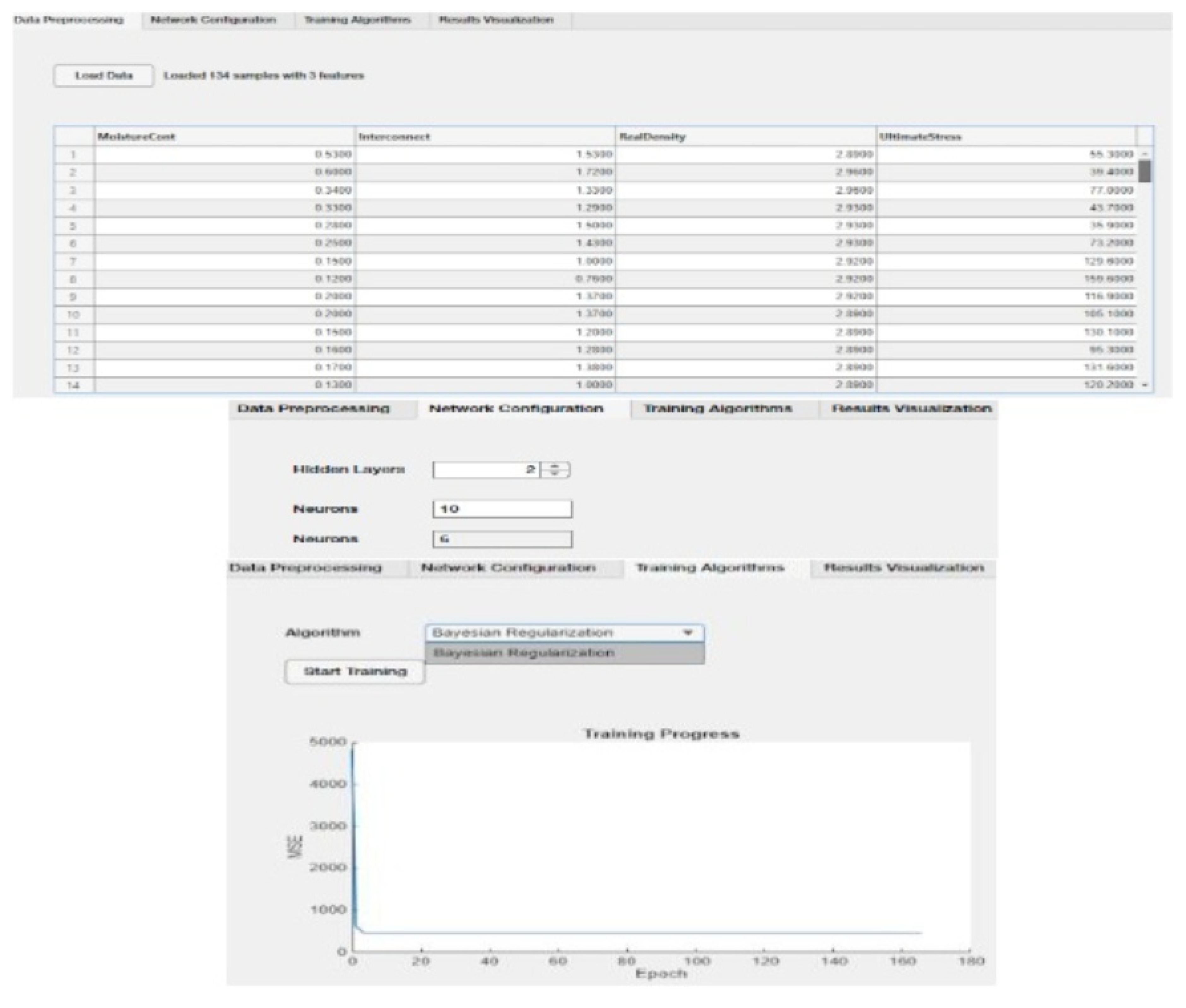
Figure 15 presents the custom Graphical User Interface (GUI) designed to facilitate Bayesian-Regularized Backpropagation Neural Network (BR-BPNN) training and evaluation. In the upper panel, users can load and inspect the dataset, which includes multiple input features (e.g., moisture content, real density) along with the output variable (ultimate stress). The middle panel depicts the network configuration options—namely the number of hidden layers and neurons per layer—while the lower panel highlights the Bayesian Regularization algorithm selection. Once training is initiated, the “Training Progress” plot appears, tracking the mean squared error (MSE) at each epoch and offering real-time feedback on model convergence.
The provided interface streamlines model development by allowing researchers to specify hyperparameters (e.g., number of hidden layers, neurons per layer) and to visually monitor the training dynamics. As shown in the “Training Progress” plot, MSE typically decreases over successive epochs, indicating iterative improvements in model performance. By incorporating Bayesian regularization, the network seeks to mitigate overfitting and promote robust generalization. Overall, this GUI simplifies the neural network workflow—from data loading and preprocessing through algorithm selection and real-time performance assessment—thereby supporting efficient, user-friendly model experimentation.
The interface integrates data handling, neural network setup, training progress visualization, prediction comparison, and performance metrics in a single, user-friendly environment. Its main components are detailed below:
Overall, this GUI is designed to streamline the entire workflow of loading data, configuring the neural network model, performing training, evaluating error metrics, and exporting the results for further interpretation. By centralizing the selection and analysis of backpropagation algorithms, the interface facilitates a robust exploration of modeling approaches for the uniaxial compressive strength (UCS) of rock materials.
10. Summary, Conclusions and Future Work
This study utilized a Bayesian-regularized feedforward neural network to predict the uniaxial compressive strength (UCS) of Seybaplaya bank rocks based on three key parameters: moisture content, interconnected porosity, and real density. The methodology involved careful data inspection and cleaning, min–max normalization, and partitioning into training, validation, and test sets. A three-hidden-layer network (10–6–1 neurons) with hyperbolic tangent activations proved effective, while Bayesian regularization (trainbr in MATLAB) balanced model complexity against data fidelity. Performance was evaluated using mean squared error (MSE), mean absolute error (MAE), and the coefficient of determination (R²), with additional diagnostic plots (actual vs. predicted, residual distributions) to quantify and visualize predictive accuracy. A purpose-built GUI further streamlined the neural network workflow, enabling intuitive data loading, algorithm selection, and training progress monitoring.
1. Feasibility of UCS Prediction
The results confirm that moisture, porosity, and density are viable predictors of UCS in heterogenous carbonate–clay rock formations, capturing a substantial portion of the compressive strength variance.
2. Benefits of Bayesian Regularization
Bayesian regularization effectively mitigated overfitting by adaptively penalizing large weights, leading to a parsimonious model that generalized well to unseen data. Indicators such as a moderate validation R² and a relatively narrow gap between training and test errors demonstrated robust generalization capacity.
3. Model Interpretability and Limitations
Linear regression analyses (slopes and intercepts) and residual plots revealed systematic underestimation at higher stress values and slight positive bias at lower levels. Although overall performance was strong, the presence of outliers and higher variance at extreme target ranges suggests room for improved feature representation.
4. GUI Implementation
The introduction of a custom GUI for Bayesian-regularized Backpropagation provided a user-friendly platform for hyperparameter configuration, real-time training feedback, and performance evaluation. This interface lowered the technical barrier to applying neural networks in geomechanical modeling.
In essence, the study validates a machine learning–based approach for predicting UCS in challenging geological settings, demonstrating both quantitative reliability and a flexible experimentation framework. However as future work:
1. Additional Geotechnical Features
Incorporating more advanced rock properties, such as mineralogical composition, micro-fracture characteristics, or ultrasonic velocity measurements, may improve the network’s ability to capture complex relationships and refine predictions.
2. Expanded Dataset
Gathering a broader and more diverse set of samples—potentially from multiple quarries or distinct lithological contexts—would help the model better handle variability and extreme values, further augmenting its generalization capacity.
3. Alternative Architectures
Exploring more sophisticated deep learning architectures (e.g., convolutional neural networks for image-based features or ensemble models) could shed light on new patterns and reduce residual errors, particularly in higher stress regimes.
4. Hybrid Modeling Approaches
Future efforts might combine this Bayesian-regularized neural network with other machine learning or statistical methods (such as Gaussian processes or random forest) to compare performance and construct ensemble predictors.
5. Sensitivity and Uncertainty Analyses
Implementing systematic sensitivity analyses of individual model inputs and advanced uncertainty quantification (e.g., Monte Carlo dropout in neural networks) can yield deeper insights into the reliability of UCS predictions and help prioritize data collection efforts.
Overall, the framework presented here lays a foundation for continuing refinement of geotechnical modeling methods, where machine learning techniques and domain-specific domain knowledge converge to enhance predictive accuracy and engineering decision-making.
Author Contributions
Jose W. Naal-Peech: Design, Experimental data measurement in si-tu, Performance of the experiments, Conceptualization, Visualization, Validation, Supervision, Writing and revision of the manuscript. Leonardo Palemón-Arcos: Project administration, Conceptualization, Visualization, Supervision, Design, Formal análisis, Writing, and revision of the manuscript. Youness El-Hamzaoui: Conceptualization, Data curation including analysis of the data, Visualization, Validation, Software, Methodology, Writing, Supervision, and revision of the manuscript.
Funding
No external funding was received for this study. However, our institution may provide support once the manuscript is accepted for publication. Otherwise, we, as the authors, will jointly cover any publication fees should our article be accepted.
Data Availability Statement
Acknowledgements
The authors, Jose W. Naal-Peech, Leonardo Palemón-Arcos, and Youness El-Hamzaoui, express their gratitude for the support provided by the Consejo Nacional de Humanidades, Ciencias y Tecnologías (CONAHCYT), the Programa para el Desarrollo Profesional Docente (PRODEP), Grupo Disciplinar Ingeniería estructural aplicada e ingeniería de la construcción y sus procesos sustentables through Universidad Autónoma del Carmen (UNACAR), and the Engineering PhD Program of Faculty of Engineering of Universidad Autónoma del Carmen (UNACAR).
Conflicts of Interest
The authors declare no conflict of interest
References
- Z. T. Bieniawski, Engineering Rock Mass Classifications: A Complete Manual for Engineers and Geologists in Mining, Civil, and Petroleum Engineering. New York, NY, USA: Wiley, 1975.
- A. Naal-Pech, J. Doe, and R. Smith. Influence of porosity and density on the compressive strength of Seybaplaya bank rocks. J. Geotech. Stud. 2023, 45, 215–227. [Google Scholar]
- ASTM International, “ASTM D7012-10: Standard Test Method for Compressive Strength and Elastic Moduli of Intact Rock Core Specimens Under Varying States of Stress and Temperatures,” West Conshohocken, PA, USA, 2010.
- J. Peng and K. Zhang. Effects of water content on the mechanical behavior of sedimentary rocks. Rock Mech. Rock Eng. 2007, 40, 125–137. [Google Scholar]
- C. Chang, T. H. R. Y. Soon, and S. McDougall. Porosity and compressive strength relationships in carbonates. Rock Mech. Rock Eng. 2006, 39, 443–456. [Google Scholar]
- M. Galván and I. Restrepo. Nonlinear relationships between water saturation and unconfined compressive strength in limestones. Int. J. Rock Mech. Min. Sci. 2016, 84, 66–74. [Google Scholar]
-
A. Naal-Pech, J. Doe, and R. Smith, “Extended correlations for UCS prediction in karstic limestones,” in Proc. 15th Int. Cong. Rock Mechanics, 2024, pp. 123–129.
- A. Gokceoglu. A comparative study of neural network and multiple regression analysis in modeling rock properties. Eng. Geol. 2002, 66, 281–295. [Google Scholar]
- M. Fener, E. Gül, and O. Ayday. Prediction of uniaxial compressive strength using artificial neural networks. Environ. Geol. 2005, 47, 101–2005. [Google Scholar]
- Naal-Pech JW, Palemón-Arcos L, El Hamzaoui Y, Gutiérrez-Can Y. Study of the relationship between uniaxial compressive strength, water content, porosity and density in bank rocks in Seybaplaya Campeche. J. Mech. Eng. 2023, 7, 9–16. [Google Scholar]
- Peng S, Zhang Z. “Correlations of compressive strength (MPa) with rock physical properties.” Petroleum Science. 2007;4(1):67–73.
- Gokceoglu, C. “A neural network application to estimate the uniaxial compressive strength of some rocks from their petrographic characteristics.” Rock Mech. Rock Eng. 2002;35(3):279–293.
- Lal, R. “Shale mechanical properties and crack propagation.” J. Petroleum Sci. 1999;6(3):235–240.
-
B. Freyburg.UCS = 0.035Vp – 31.5: A correlation with ultrasonic velocity speed. 1972. [Unpublished/Technical Note; confirm source].
- G. H. McNally. “Estimation of coal measures rock strength using sonic and density logs.” Log Analyst. 1987;28:20–27.
- Chang C, et al. “Empirical relationships between compressive strength and porosity in Gulf of Mexico rocks.” SPE J. 2006;11(1):19–25.
- Naal-Pech JW, Palemón-Arcos L, El Hamzaoui Y, Gutiérrez-Can Y. “Study of the relationship between uniaxial compressive strength and the point load test in rocks from the bank in Seybaplaya Campeche Mexico.” J. Eng. Appl. 2024;11(32):36–42.
-
Galván M, Restrepo I. “Correlación de la resistencia a compresión uniaxial con la humedad y porosidad eficaz en rocas.” DYNA. 2016. [In Spanish; verify volume/pages if available].
- Naal-Pech JW, Palemón-Arcos L, El Hamzaoui Y, Gutiérrez-Can Y. “Study of the relationship between uniaxial compressive strength and the indirect tensile test (BTS) in rocks from the bank in Seybaplaya Campeche Mexico.” ECORFAN J.-Bolivia. 2024;11(21):26–33.
- B. Militzer and R. D. Stoll. “Effect of lithology and pore fluids on compressional wave velocity in carbonates.” Geophysics. 1973;38(2):341–350.
- Naal-Pech JW, Palemón-Arcos L, El Hamzaoui Y, Gutiérrez-Can Y. “Study of the relationship between uniaxial compressive strength vs non-destructive testing and specific weight in bank rocks in Seybaplaya Campeche Mexico.” J. Eng. Appl. 2024;11(31):16–25.
-
Palemón-Arcos L, Naal-Pech JW, El Hamzaoui Y, Gutiérrez-Can Y. “Observations on lithological discontinuities and water infiltration in limestone benches of Seybaplaya.” [Conference paper or journal article, 2023; confirm final citation details].
- S. Kahraman. “Evaluation of simple methods for assessing the uniaxial compressive strength of rock.” Int. J. Rock Mech. Min. Sci. 2001;38:981–994.
- Fener M, Kahraman S, Bilgili A, Gunaydin O. “A comparative evaluation of indirect methods to estimate the compressive strength of rocks.” Rock Mech. Rock Eng. 2005;38(4):329–343.
- Gokceoglu C, Zorlu K. “A fuzzy model to predict the unconfined compressive strength and modulus of elasticity of a problematic rock.” Eng. Appl. Artif. Intell. 2004;17:61–72.
- Bishop, CM. Neural Networks for Pattern Recognition. Oxford University Press; 1995.
-
LeCun Y, Bengio Y, Hinton G. Deep learning. Nature. 2015;521(7553):436–444.
-
MacKay DJC. Bayesian interpolation. Neural Comput. 1992;4(3):415–447.
-
Rumelhart DE, Hinton GE, Williams RJ. Learning internal representations by error propagation. In: Rumelhart DE, McClelland JL, editors. Parallel Distributed Processing: Explorations in the Microstructure of Cognition. vol. 1. MIT Press; 1986. p. 318–362.
-
Chang C, Soon THR, McDougall S. Porosity and compressive strength relationships in carbonates. Rock Mech Rock Eng. 2006;39(5):443–456.
- Kohavi, R. A study of cross-validation and bootstrap for accuracy estimation and model selection. In: Proceedings of the 14th International Joint Conference on Artificial Intelligence (IJCAI); 1995. p. 1137–1145.
-
Gokceoglu C, Zorlu K. A fuzzy model to predict the unconfined compressive strength and modulus of elasticity of a problematic rock. Eng Appl Artif Intell. 2004;17(1):61–72.
-
Gokceoglu C. A neural network application to estimate the uniaxial compressive strength of some rocks from their petrographic characteristics. Rock Mech Rock Eng. 2002;35(3):279–293.
- MATLAB. Neural Network Toolbox: User’s Guide. Natick, MA: The MathWorks, Inc.; 2024.
Figure 1.
histograms for MoistureCont, Interconnecte, RealDensity, and UltimateStress.
Figure 1.
histograms for MoistureCont, Interconnecte, RealDensity, and UltimateStress.
Figure 2.
boxplots for each of the four primary variables—Moisture Cont (MoistureCont), Interconnecte (porosity), Real Density (RealDensity), and Ultimate Compressive Strength (UltimateStress).
Figure 2.
boxplots for each of the four primary variables—Moisture Cont (MoistureCont), Interconnecte (porosity), Real Density (RealDensity), and Ultimate Compressive Strength (UltimateStress).
Figure 3.
Correlation matrix for the four principal variables: MoistureCont, Interconnecte (porosity), RealDensity, and UltimateStress (UCS).
Figure 3.
Correlation matrix for the four principal variables: MoistureCont, Interconnecte (porosity), RealDensity, and UltimateStress (UCS).
Figure 4.
scatter plot matrix for the four primary variables—MoistureCont, Interconnecte, RealDensity, and UltimateStress.
Figure 4.
scatter plot matrix for the four primary variables—MoistureCont, Interconnecte, RealDensity, and UltimateStress.
Figure 5.
Parallel coordinate plot.
Figure 5.
Parallel coordinate plot.
Figure 6.
Optimal Deep learning architecture.
Figure 6.
Optimal Deep learning architecture.
Figure 7.
Training Progress of the Bayesian-Regularized Backpropagation Neural Network.
Figure 7.
Training Progress of the Bayesian-Regularized Backpropagation Neural Network.
Figure 9.
Residual plot for the best-performing Bayesian-regularized neural network.
Figure 9.
Residual plot for the best-performing Bayesian-regularized neural network.
Figure 14.
Regression Analysis of Neural Network Performance Across Training, Validation, and Test Datasets with Corresponding Correlation Coefficients.
Figure 14.
Regression Analysis of Neural Network Performance Across Training, Validation, and Test Datasets with Corresponding Correlation Coefficients.
Figure 15.
Graphical User Interface for Neural Network Training and Comparative Evaluation of Backpropagation Algorithms.
Figure 15.
Graphical User Interface for Neural Network Training and Comparative Evaluation of Backpropagation Algorithms.
Table 1.
Statistical interpretation (mean, standard deviation, min, median, max).
Table 1.
Statistical interpretation (mean, standard deviation, min, median, max).
| Variable |
Mean |
StdDev |
Min |
Median |
Max |
| MoistureCont |
3.8011 |
3.0442 |
0.08 |
3.965 |
13.62 |
| Interconnecte |
6.5263 |
7.4131 |
0.31 |
1.37 |
28.46 |
| RealDensity |
2.4943 |
0.2251 |
1.91 |
2.45 |
2.96 |
| UltimateStress |
60.128 |
29.815 |
8.60 |
53.83 |
159.60 |
Table 2.
Correlation coefficient matrix (r-values).
Table 2.
Correlation coefficient matrix (r-values).
| Variables |
MC (MoistureCont) |
IC (Interconnecte) |
RD (RealDensity) |
UCS (UltimateStress) |
| MC (MoistureCont) |
1.0000 |
0.8530 |
-0.7620 |
-0.6242 |
| IC (Interconnecte) |
0.8530 |
1.0000 |
-0.5755 |
-0.5188 |
| RD (RealDensity) |
-0.7620 |
-0.5755 |
1.0000 |
0.6641 |
| UCS (UltimateStress) |
-0.6242 |
-0.5188 |
0.6641 |
1.0000 |
Table 3.
p-values matrix for correlation significance.
Table 3.
p-values matrix for correlation significance.
| Variables |
MC (MoistureCont) |
IC (Interconnecte) |
RD (RealDensity) |
UCS (UltimateStress) |
| MC (MoistureCont) |
1.0000 |
0.0000 |
0.0000 |
0.0000 |
| IC (Interconnecte) |
0.0000 |
1.0000 |
0.0000 |
0.0000 |
| RD (RealDensity) |
0.0000 |
0.0000 |
1.0000 |
0.0000 |
| UCS (UltimateStress) |
0.0000 |
0.0000 |
0.0000 |
1.0000 |
Table 4.
Summary statistics of normalized features across all samples.
Table 4.
Summary statistics of normalized features across all samples.
| |
Moisture |
Porosity |
Density |
| Mean |
0.27482 |
0.22083 |
0.55643 |
| StdDev |
0.22483 |
0.26334 |
0.21438 |
| Min |
0 |
0 |
0 |
| Max |
1 |
1 |
1 |
Table 5.
Validation mean squared error (MSE) and coefficient of determination (R2) for each run.
Table 5.
Validation mean squared error (MSE) and coefficient of determination (R2) for each run.
| Run |
Validation MSE |
Validation R2
|
| 1/5 |
652.7979 |
0.4299 |
| 2/5 |
642.4685 |
0.4389 |
| 3/5 |
639.1605 |
0.4418 |
| 4/5 |
674.7770 |
0.4107 |
| 5/5 |
431.1431 |
0.5670 |
Table 6.
Final chosen network performance on training and test subsets.
Table 6.
Final chosen network performance on training and test subsets.
| |
MSE |
RMSE |
MAE |
R2
|
| Train |
431.1431 |
20.7640 |
16.7634 |
0.5670 |
| Test |
590.4544 |
24.2993 |
20.7947 |
0.4626 |
|
Disclaimer/Publisher’s Note: The statements, opinions and data contained in all publications are solely those of the individual author(s) and contributor(s) and not of MDPI and/or the editor(s). MDPI and/or the editor(s) disclaim responsibility for any injury to people or property resulting from any ideas, methods, instructions or products referred to in the content. |
© 2025 by the authors. Licensee MDPI, Basel, Switzerland. This article is an open access article distributed under the terms and conditions of the Creative Commons Attribution (CC BY) license (http://creativecommons.org/licenses/by/4.0/).