Submitted:
17 January 2025
Posted:
17 January 2025
You are already at the latest version
Abstract
This paper proposes an obstacle avoidance strategy for an underwater robot that integrates Hidden Markov Chains (HMC) with a fuzzy controller. The HMC predicts a vector of future states, leveraging the maximum state probabilities to guide the behavior of the fuzzy controller. The proposed fuzzy controller utilizes five inputs: the robot’s state predictions (crisp sets), instantaneous linear velocity, underwater depth, and yaw and pitch velocities, modeled with Gaussian and sigmoid membership functions. It generates three outputs, also using Gaussian and sigmoid functions, corresponding to the robot’s actuators: the propulsion motor, the steering motor, and the ballasting motor, which operates through an integrated hydraulic piston system. The paper also develops physics-based models for the propulsion, steering, and ballasting systems, alongside sensor fusion models that provide real-time control feedback. Additionally, it presents the robot’s platform and system architecture, designed with multi-threaded, real-time control capabilities. Experimental and simulation results validate the effectiveness of the proposed strategy, demonstrating robust obstacle avoidance in underwater navigation.
Keywords:
underwater-robotics
; Markov-Decision
; Fuzzy-control
; model-based-control
; intelligent-navigation
; smart-obstacle-avoidance
; robot-architecture
1. Introduction
In recent years, the field of mobile robotics has seen significant advancements, particularly in the domain of underwater exploration. Autonomous Underwater Vehicles (AUVs) represent a cutting-edge class of mobile robots, uniquely designed to navigate the complex underwater environment with a wide range of intelligent functionalities. A review of underwater robotic functionalities such as localization, navigation and multiple sensing techniques can be found in [1]. AUVs are distinguished from Remotely Operated Vehicles (ROVs) by their ability to operate independently without direct human intervention. Unlike ROVs, which require a tethered connection to a surface vessel, AUVs are powered by their own onboard energy sources, allowing them greater freedom and versatility in their operations. The impetus for advancing AUV technology primarily stems from the need to collect vital oceanographic data, including measurements of temperature, salinity, and ocean currents. These vehicles play a crucial role in inspecting underwater infrastructures such as pipelines, submarine cables, and oil platforms. Beyond these applications, AUVs are instrumental in generating high-resolution bathymetric maps and aiding in the discovery and exploration of sunken vessels. They are invaluable assets in marine biological research, providing insights into marine life and underwater ecosystems. Additionally, they serve important purposes in surveillance and reconnaissance missions.
The development of UAVs in experimental environments with real-time performance and planning algorithms presents significant challenges. Achieving stability requires addressing critical factors such as real-time pathfinding algorithms, dynamic obstacle avoidance, path optimization, and sufficient processing speed, particularly when contending with hydrodynamic currents. A comprehensive review of these issues was presented by Li et al. [2]. Kot et al. [3] reviewed two decades of research on collision avoidance and path planning for AUVs, comparing simulations with real-world implementations. They found that real-world applications predominantly rely on simpler, reactive behaviors.
This research presents an obstacle avoidance strategy for an underwater robot by integrating Hidden Markov Chains (HMC) with a fuzzy controller. The purpose of the HMC approach is to predict the robot’s next action for real-time obstacle evasion. The output of the HMC provides inferred states that serve as critical input to one of the fuzzy sets in the fuzzy controller, which estimates numerical values for the robot’s actuators. The proposed fuzzy controller incorporates five inputs: the robot’s state prediction quantized by crisp sets, instantaneous linear velocity, underwater depth, yaw velocity (angular azimuth), and pitch velocity (elevation angle), using a mix of Gaussian and sigmoid membership functions. Feedback information is obtained from ultrasonic sensors positioned at the six cardinal points (front, back, left, right, down, and up), a three-axis gyroscope, a three-axis accelerometer, and a liquid pressure sensor. The fuzzy controller generates three outputs, with a combination of Gaussian and sigmoid functions, one for each of the robot’s actuators: the propulsion motor, steering motor, and a ballasting motor integrated into a hydraulic piston system. These outputs are interpreted by optical encoders that measure the motors’ rotary information. Physics-based models for the propulsion, steering, and ballasting systems are developed, along with sensor fusion models that enable control feedback. Additionally, the paper introduces the robot’s platform and system architecture. Experimental and numerical simulation results demonstrate the effectiveness of the proposed strategy in achieving robust obstacle avoidance for underwater navigation. As an initial validation, experimental results are presented using a prototype tested in a pool, assuming an ideal static fluid without external hydrodynamic forces.
Section 2 reviews relevant state-of-the-art works. Section 3 describes the architecture and design of the robotic platform architecture. Section 4 derives deterministic models for the robot’s actuators and sensors. Section 5 describes the hidden Markov chain model that predicts the robot’s state transitions for obstacle avoidance. Section 6 provides a comprehensive description of the fuzzy navigation control system. Section 7 deduces the kinematics and dynamics of the robotic submarine’s motion actuators. Finally, Section 8.
2. Related Work
The work reported by Cheng et al. [4] reviewed the growing importance of autonomous underwater vehicles (AUVs) in marine exploration, emphasizing path planning and obstacle avoidance. Their work provides a comprehensive overview of existing path planning methods, classifying them as global or local based on obstacle awareness, and offers valuable insights for new researchers and future research directions. In their work, Xu et al. [5] presented a comprehensive analysis of path planning technologies employed in autonomous underwater vehicle (AUV) missions. The authors reviewed a spectrum of algorithms, encompassing both traditional and intelligent methodologies, providing a comparative assessment of their respective advantages and limitations.
Chen et al. [6] conducted real-world experiments on underwater obstacle avoidance using a Remotely Operated Vehicle (ROV). Fuzzy logic controlled the ROV’s depth and heading based on sensor data, with sonar aiding in heading adjustments. This approach ensured control stability and effective obstacle avoidance. Lin et al. [7] proposed a recurrent ANN with convolution for online obstacle avoidance in UUVs, focusing on feature extraction with reduced parameters. This method utilizes sonar and deep learning techniques. Bhopale [8] proposed a model-free reinforcement learning approach to adapt to environmental changes without manual tuning, using an ANN for state approximation for AUV obstacle avoidance in unknown environments. The stydy of Yang et al. [9] proposed a novel path planning solution for underwater robots using an N-step Priority Double DQN algorithm. This approach effectively addresses dynamic obstacle avoidance in realistic 3D underwater environments, incorporating real ocean current data. By introducing an experience screening mechanism, the algorithm enhances stability and adaptability without relying on prior experience.
Research by [10] proposed an obstacle avoidance approach for submarine robots centered on a ’motion balance point’, aimed at long operation times and high energy efficiency. It combined local obstacle avoidance planning, control, and hydrodynamics, tracking dynamic obstacle avoidance through models of velocity, acceleration, and Singer acceleration. Zhang [11] discusses improving real-time obstacle avoidance in underwater robots using an enhanced artificial potential field method to address collision and path smoothness issues. The method employs a dynamic adjustment factor implemented in ROS, demonstrating effective real-time obstacle avoidance. The work of [12] introduced a 3-D obstacle avoidance algorithm for Autonomous Underwater Vehicles (AUVs) using the sphere cross-section method, employing Dubins-like curves for smooth trajectory planning. Yan et al. [13] proposed a real-time reactive obstacle avoidance algorithm for AUVs using forward-looking sonar. The algorithm simplifies obstacle outlines to convex polygons and introduces a memory-based solution for handling U-shaped obstacles. Wu [14] developed a dynamic obstacle avoidance method for AUVs within a velocity vector coordinate system, particularly for deep-sea exploration. This method addresses the complex relationship between velocity and displacement.
Yao [15] proposed a control method for AUVs to track 3D linear paths while avoiding obstacles. This method combines kinematic model predictive control with a dynamic controller utilizing sliding mode control to improve waypoint path tracking, reduce angle errors, and prevent saturation. Sun et al. [16] developed a control algorithm combining model predictive control for trajectory replanning and obstacle avoidance with sliding mode control for robust trajectory tracking in uncertain underwater environments, ensuring effective obstacle avoidance and stable tracking while reducing thruster saturation. Yu [17] proposes a robust nonlinear model predictive control scheme for high-speed waypoint tracking and real-time obstacle avoidance in large-scale, underactuated AUVs operating in unknown environments. It includes a dynamic sensing and collision avoidance scheme that transforms nonconvex obstacles into convex constraints. Li et al. [18] proposed a strategy that combines an enhanced A* algorithm with Model Predictive Control to improve path planning and obstacle avoidance for Unmanned Underwater Vehicles (UUVs). This approach uses a kinematic and dynamic UUV model for 3D path planning and supports real-time re-planning for dynamic obstacles.
3. Robotic Platform
This section provides a comprehensive overview of the development and design of the underwater robotic platform’s architecture deployed experimentally in this research. It outlines the construction of the mechanical physical system and electronic instrumentation, alongside the modular design of the robot’s components. The software modules are elaborated at a multithread level to enable real-time operations. Additionally, the development of Autonomous Underwater Vehicles (AUVs), Remotely Operated Vehicles (ROVs), or Unmanned Underwater Vehicles (UUVs) can yield cost-effective robotic vehicles focused on robotics research, which may be achieved with a low-cost design approach, as referenced in [19].
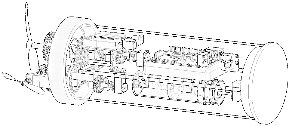
Figure 1a depicts three main views of the proposed robot: rear, top, and lateral, along with their corresponding planes and Cartesian axes. It also shows the location of proprioceptive sensors such as an inertial measurement unit (IMU), a pressure sensor, and an exteroceptive sensor Red-Green-Glue Depth (RGBD) (not covered in this manuscript). Additionally, a graphical representation of other exteroceptive sensors, such as the acoustic cones of ultrasonic sonars is illustrated, situated along the six cardinal axes: front and back (), up and down (), and left and right ().
In addition, Figure 1b shows a photo of the robotic submarine that was developed to carry out the experimental issues of this research.
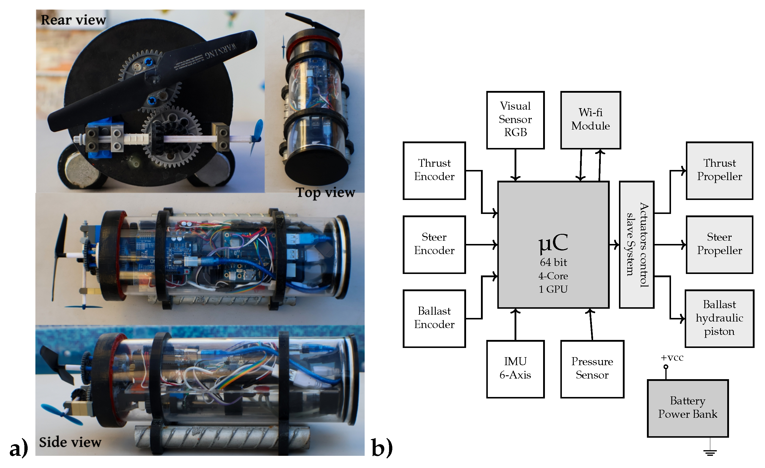
Figure 2 illustrates the modular-level instrumentation diagram of the robotic architecture design (Figure 2b). It includes two electronic boards: the Orange PI, a 64-bit, quad-core 1.5 GHz RISC mini-computer serving as the master system, and an Arduino ATmega328P control and sensing module card acting as the slave computer. The master computer primarily coordinates and synchronizes sensory data and control signals to the actuators.
The three actuators (propulsion, steering, and ballast) are DC motors controlled via pulse width modulation (PWM), with feedback provided by rotation data through pulse encoder integration. The master computer runs a 64-bit Linux operating system equipped with matrix calculation libraries and manages WiFi ports for TCP/IP communication.
Additionally, Figure 2a presents illustrations of the transparent chassis with the master-slave board assembly and other instrumentation devices.
The computational architecture of the robot is designed as a real-time system leveraging a multi-threaded framework to support concurrent execution of various processes. These processes are categorized into three primary classes:
- a.
- Sensing threads: Responsible for acquiring and preprocessing data from the robot’s sensors in real-time.
- b.
- Control and actuation threads: Handle decision-making and command transmission to the robot’s actuators, ensuring responsive and precise execution of tasks.
- c.
- Computation and planning threads: Perform intensive arithmetic and logical calculations, such as trajectory planning and optimization algorithms.
To enable seamless inter-thread communication and coordination, the system employs shared memory techniques coupled with mutual exclusion mechanisms to prevent data conflicts and ensure thread-safe operations. This structure allows for efficient real-time data flow and processing, crucial for the robot’s functionality in dynamic environments.
The entire system, including all threads and routines, was implemented in C/C++ using the GNU Compiler Collection (GCC). To ensure a robust, efficient, and portable foundation for resource management and real-time operations, the implementation adhered to the POSIX standard, leveraging features within the C++ standard library. This approach facilitated the development of a clean, well-structured, and maintainable codebase.
For computational tasks involving numerical linear algebra and matrix operations, the Armadillo C++ library was employed, providing a high-performance and user-friendly interface. Additionally, real-time visualization of experimental data during runtime was seamlessly integrated using the Sciplot library, enabling dynamic and interactive monitoring of the system’s performance.
The algorithms executed within the threads operate at varying frequencies, tailored to the specific requirements of each process. These threads interact with reserved memory locations to read and write data, ensuring efficient data management and coordination. Synchronization mechanisms are employed to seamlessly integrate these operations, enabling precise low-level control of the actuators while simultaneously handling large volumes of data from the sensors. This architecture ensures real-time responsiveness and robust system performance, even in data-intensive and dynamic environments.
4. Sensor and Actuator Models
This section describes the sensor and actuator configuration relevant to the obstacle avoidance task. While the experimental robot prototype incorporates a comprehensive array of sensors, only those directly pertinent to the scope of this manuscript are presented herein. Specifically, the system employs optical incremental encoders for precise measurement of motor shaft angular displacement, an inertial measurement unit (IMU) integrating a three-axis gyroscope and a three-axis accelerometer for inertial navigation, and a pressure sensor for depth determination. The optical encoders operate as transducers, converting the continuous rotational motion of the motor shafts into a discrete pulse train at TTL voltage levels.
4.1. Observation Models
An observer model, commonly referred to as an observer, is a mathematical representation of a system designed to estimate its internal states based on observed inputs and outputs. In real-world robotics applications, such as the one discussed in this manuscript, it is often impractical or impossible to directly measure all internal states of the system.
Sensor measurements are typically noisy and influenced by various factors, such as environmental interference and inherent sensor inaccuracies, which can compromise the reliability of the readings. Observers address these challenges by leveraging a system model to estimate states that are either unmeasurable or significantly affected by noise. This approach enhances the overall accuracy and robustness of state estimation, enabling more effective system control and decision-making.
Therefore, we initially consider the angular velocity model derived by an optical encoder from the rotational motion of each motor, such that:
Here, represents the instantaneous number of pulses measured by the encoder, while R is a constant defining the encoder’s resolution in pulses per revolution. Both parameters are dimensionless. Here, represents the observation, rather than a measurement. Based on this, the following Proposition 1 is established.
Proposition 1
(Encoder’s rotary velocity). The numerical derivative is defined using the backward divided difference method, truncated through the Taylor series expansion. This approach allows for a high-precision calculation of the derivative as a function of time:
By substituting the encoder model at different points in time, we derive an expression that depends on the number of pulses measured by the encoder and the corresponding time:
Here, represents the time interval used for the control and sampling cycle.
Therefore, Proposition 1 applies generally for any of the robot’s rotary actuators: propulsion, steer and ballast.
The robot’s proprioceptive motion measurements were conducted using an IMU that comprises a three-axis gyroscope and a three-axis accelerometer. These components are utilized for inferring observations across various physical units. Fundamentally, measurements of Euler angles and Cartesian accelerations were taken, with the IMU centrally positioned at the midpoint of the submarine.
The roll (), pitch (), and yaw () angles, as well as the angular acceleration around the axes, are inferred from the raw gyroscope data. To estimate any Euler rotation angle, the trapezoidal integration method was employed. This approach is a precise online numerical calculation method and becomes more accurate as the number of segments increases.
where n is the number of samples accumulated between and . are the time integration limits.
Besides, the angular accelerations observations are estimated by
where is the measured time of data sampling.
Moreover, the linear accelerations of the robot’s body under inertial effects is measured by the accelerometer devices, and the linear velocity is inferred by
Additionally, the pressure transducer, when subjected to a hydraulic load, requires a calibration model, such that
where is the absolute pressure. is the atmosphere pressure. is a measurement of atmosphere pressure just above the water surface, and is the the measurement of the transducer at an arbitrary underwater depth.
Therefore, the instantaneous underwater pressure is inferred by the following observer model,
The ultrasonic sonar, which measures the distance between the robot’s main points and obstacles, is set within a unified coordinate system anchored to the robot’s center. All obstacles are represented in Cartesian coordinates as . According to Figure 1a, the front () and back () sonars are longitudinally aligned along the x-axis. The left () and right () sonars are transversely aligned along the y-axis. The bottom () and top () sonars are vertically aligned along the z-axis.
All components measured by each sonar transducer on the horizontal -plane, are inferred by
and
Likewise, considering the vertical -plane the z component is obtained by
where, is the orientation angle of each sonar sensor, such that , and . In addition, over the -plane .
4.2. Rotary Actuators
This section details the derivation of the kinematic model for the DC motors responsible for robot actuation. To address the influence of hydrostatic pressure on motor performance, particularly potential reductions in rotational power with increasing depth, a third-degree polynomial adaptive adjustment model is proposed. This model aims to dynamically compensate for these losses and maintain the desired motor speed.
The primary strategy is to develop an empirical model of each motor’s kinematic behavior. This empirical model comprises experimental data as a tuple, including the motor’s angular velocity correlated with a specified digital word (dimensionless), which is obtained through a controlled experiment. The digital word refers to a natural number linked to varying pulse width modulation (PWM) frequencies. By writing a digital word to the computer’s PWM port, a desired motor velocity is set. Upon acquiring the empirical model, as illustrated in Figure 3, a theoretical model is then derived.
This theoretical model is a mathematical function that closely replicates the real empirical model with higher precision. Additionally, the empirical model can be further analyzed mathematically.
The plot Figure 3 illustrates the experimental performance of the propulsion and sterring motors angular velocity in relation to their digital control word (PWM).
Hence, the regression model that optimally approximates the empirical model is represented by the following system in Equation 10, derived utilizing the least squares method.
where n is the total number of experimental data. Thus, estimating the coefficient of interest, algebraically arrange for the inverse solution,
The polynomial representation for motor velocity control as a function of is expressed as:
This implies that the digital output is estimated in relation to a specified angular velocity.
5. Robot’s State Prediction
This section describes the proposed Hidden Markov Chain (HMC) model for predicting seven process states of a submarine robot to avoid obstacles. Probabilities in each state are calculated based on separate observations, which are the distances measured by six proximity sensors positioned at the robot’s cardinal points. The purpose of this approach is to predict the robot’s next action tasks for obstacle evasion in real-time. The output of the HMC are inferred states that serve as critical input to one of the fuzzy sets in the fuzzy controller, which estimates numerical values for the robot’s actuators (see Section 6). The proposed HMC features a non-stationary stochastic state transition matrix, where state transition probabilities change instantaneously according to probability observations as functions of obstacles proximity. During state prediction, the probabilities of hidden states are calculated, and the state with the highest probability at the current time is used as the input to the fuzzy controller.
A hidden Markov chain is a statistical model used to represent systems that transition between states in a Markov process, where the states themselves are not directly observable (hidden). Instead, you can observe a sequence of outputs or emissions, which are probabilistically related to the underlying hidden states. Hidden states are the states the system transitions through, which are not directly visible. The observations are the observable sensor data.
The transition probabilities or for simplicity notation , define the likelihood of transitioning from one hidden state to another. The emission probabilities represent the probability of a particular hidden state.
The study by Brito et al. [20] presented a Markov chain-based approach to model the sequential steps of autonomous underwater vehicle (AUV) missions, from prelaunch to recovery, with the goal of identifying high-risk states and transitions. The model outlines event sequences and assigns transition probabilities across 11 discrete states, incorporating distance-dependent survival statistics. Additionally, the study by Ali et al. [21] introduced a deep learning approach utilizing a network for real-time state estimation of underwater maneuvering objects within a Markov chain framework. It evaluates the network’s performance in bearings-only tracking under various ocean conditions and noise levels.
The elements depicted in Figure 4 represent all the states of the chain and their respective transitions, as detailed in Table 1. Define to denote the transitions between the robot’s states. The functions represent the probability of each state occurring, while the probabilities indicate the likelihood of distinct output observations. Additionally, represents the probability of transitioning between states and .
Definition 1
(Transition from any to ). Let that represent the probability model describing transitions from any of the states toward the state . The model serves as an alternative to the inverse exponential probabilities and is defined as:
where are the distances measured to an obstacle by the ranging sensor, and is an adjustment parameter that determines the amplitude and range of the probability based on the proximity of obstacles to the robot. This definition captures the scenario in which all sensors detect obstacles in their respective directions (cardinal points), influencing the robot to transition toward the state .
In addition, there is another important Definition 2.
Definition 2
(Probability of current state transition ). Let represent the inverse exponential probability model describing transitions from current state toward the same state . The model serves as an alternative to the inverse exponential probabilities and is defined as:
where is the distance measured to an obstacle by the ranging sensor, and is an adjustment parameter that determines the amplitude and range of the probability of state based on the proximity of obstacles to the robot. This definition describes a scenario in which the robot remains in its current state, , when no obstacles influence that state. In this case, the complement of the transition probability is inversely proportional to the presence of obstacles, resulting in a high likelihood for the robot to stay in the same state.
The Markov state transition stochastic matrix , as referenced in Definitions 1 and 2, assumes a probability when the measured obstacle range is approximately zero, . Therefore, we have:
For analysis purposes, let us assume . The proposed function trend is an inverse exponential where the maximum distance for obstacle detection is set to 5 meters. The Markov state transition stochastic matrix is a non-stationary matrix model that is updated at each control loop based on range sensor measurements. Consequently, its dynamic elements change according to the following inverse exponential functions:
where are range measurements, such that is a measurement of the back-side sensor, is from the front-side sensor, and are from the right-hand and the left-hand sensors, and , are measurements from up-side and down-side sensors.
Example 1.
In an aquatic scenario, the robot senses an obstacle directly above it at a distance of m. The robot is in two initial states when detecting the obstacle above: moving forward () and simultaneously surfacing (). The Markov state transition prediction process is illustrated by Figure 5, showing only the main involved states for simplicity.
The prediction at discrete time for the state vector is established
such that, the normalized state transition vector becomes
where the prediction states that as the robot detects an obstacle above of it, then now the Markov prediction process establishes that there is now a to continue forward () and a to move downward in order to safety avoid the above obstacle. Nevertheless, for a second state prediction, at the state transition vector is
The Markov state transition process for the submarine robot indicates that there is a significant likelihood of % for the robot to ’sink’ in order to avoid the obstacle above. Additionally, there is a % chance to continue moving forward and safely avoid the obstacle. Hence, the most critical state to consider as an input for the fuzzy set of tasks is the ’sink’ prediction.
Example 2.
In a typical scenario, the underwater robot initially advances with current state `forward’() and detects an obstacle obstructing its frontal area a few meters ahead, primarily on the left (m) and near the water surface, a fraction of meter above (m). As a result, the robot maneuvers by diving and subtly turning to the right, allowing the obstacle to remain on the surface.
The Markov chain state transitions for diving towards the right side are shown in Figure 6.
Initially, the stochastic transition state vector is given by . Consequently, the subsequent prediction is obtained at the first computation as .
Thus, the state transition probabilities were estimated as follows: (stop), (forward), (backward), and (sink) during the first computation loop, which corresponds to a time period of 3 seconds. The Markov chain indicates that the robot should perform a backward propulsive motion () to avoid the front-side obstacle at 0.25m, and initiate a descent () to evade the obstacle located 0.3m above its path. Subsequently, at discrete time , the state predictions evolve as follows:
The Markov state transition process for the submarine robot indicates a probability of moving backward to avoid the nearest obstacle in front. Similarly, there is a likelihood of diving to evade an overhead obstacle. Consequently, the ’backward’ prediction is the most crucial state to consider as input for the next stage, which involves the fuzzy set of tasks.
6. Fuzzy Motion Control
This research proposes a fuzzy controller for adjusting the three motors speeds (drive, steer and ballast) taking as inputs five distinct fuzzy inputs, that include the Markov chain robot’s avoidance prediction (crisp sets), the robot’s linear and angular velocities, as well underwater depth, azimuth, and elevation angles. This approach allows the fuzzy controller to dynamically adjusting the temporal parameters to govern the movements of the underwater robot. In other reported works, David et al. [22] introduced a fuzzy logic-based controller for autonomous navigation and heuristic obstacle avoidance in unmanned underwater vehicles (UUVs) equipped with six thrusters for precise motion control and heading correction. Similarly, Peng et al. [23] developed a fuzzy logic guidance scheme for an autonomous underwater vehicle (AUV), utilizing multi-directional thrusters and adaptively adjusting the navigation coefficient.
The proposed controller is characterized as a multiple-input (five) multiple-output (three) governing system. The robot can execute seven distinct motion tasks to avoid obstacles, which are categorized by the first input fuzzy set (Figure 8a): stop, move forward, move backward, turn left, turn right, dive (sink), and surface (rise). For this first fuzzy variable, we present Definition 3, which elaborates on the parametric structure of the input sets.
Definition 3
(Input fuzzy tasks). The output of the Markov network is mapped to a fuzzy input denoted as . This represents the state transition prediction, maximizing the Markov network’s probabilistic calculation. These values are constrained to the discrete set , and their membership in this crisp set is denoted by .
The submarine robot’s sensor observations utilize sigmoid membership functions to model the S-shaped sets of both thrust speed υ [cm/s] and angular speed ω [rad/s]. This consistent modeling approach captures the extreme characteristics of both input variables.
Let denote the sets categorized as ’normal’, ’slow’, and ’fast’. These sets are prefixed with either ’n’ for negative or ’p’ for positive direction, corresponding to the push velocity υ, defined by:
where x is any of the physical variables () and a is an adjustment parameter.
Similarly, the sigmoid functions with respect to the input physical variable with adjustment parameter b is modeled as:
Moreover, the remaining intermediate sets can be described as any of the Gaussian membership functions corresponding to the robot’s kinematic variables, characterized by a parametric mean value and a standard deviation .
Consequently, the reasoning rules articulated within the inference engine have been designed by applying the fuzzy inputs, specifically tailored to produce desired outputs that correspond to the underwater motion variables of the underwater robot (refer to Figure 9). These inference rules form the most basic core decision-making engine for obstacle avoidance. However, still numerous additional rules can be included to sophisticate the avoidance planning.
Specifically, for the crisp set of avoidance tasks, the rules are abbreviated as follows: S (stop), F (forward), B (backward), L (left turn), R (right turn), D (sink or dive), and U (rise or surface). Moreover, the crisp input , a scalar component of the Markov state prediction vector, is evaluated based on the maximal value for certain inference rules, whereas other rules utilize the two or three largest values.
- if ∧ ∧ ∧ ∧ then ∧ ∧.
- if ( ∧) ∧ ∧ ∧ ∧ then ∧ ∧.
- if ( ∧) ∧ ∧ ∧ ∧ then ∧ ∧.
- if ∧ ∧ ∧ ∧ then ∧ ∧.
- if ( ∧) ∧ ∧ ∧ ∧ then ∧ ∧.
- if ( ∧ ) ∧ ∧ ∧ ∧ then ∧ ∧.
- if ∧ ∧ ∧ ∧ then ∧ ∧.
- if ( ∧) ∧ ∧ ∧ ∧ then ∧ ∧.
- if ( ∧ ) ∧ ∧ ∧ ∧ then ∧ ∧.
- if ∧ ∧ ∧ ∧ then ∧ ∧.
- if ( ∧ ) ∧ ∧ ∧ ∧ then ∧ ∧.
- if ( ∧ ) ∧ ∧ ∧ ∧ then ∧ ∧.
- if ∧ ∧ ∧ ∧ then ∧ ∧.
- if ( ∧ ) ∧ ∧ ∧ ∧ then ∧ ∧.
- if ( ∧ ) ∧ ∧ ∧ ∧ then ∧ ∧.
- if ∧ ∧ ∧ ∧ then ∧ ∧.
- if ( ∧ ) ∧ ∧ ∧ ∧ then ∧ ∧.
- if ( ∧ ) ∧ ∧ ∧ ∧ then ∧ ∧.
- if ∧ ∧ ∧ ∧ then ∧ ∧.
- if ( ∧ ) ∧ ∧ ∧ ∧ then ∧ ∧.
- if ( ∧ ) ∧ ∧ ∧ ∧ then ∧ ∧.
Therefore, the output fuzzy sets outline the rotary speeds of the robotic submarine’s propels and ballasting actuators, as illustrated in Figure 9.
The inference engine rules define the application of fuzzy operators used to evaluate the terms involved in fuzzy decision-making. For any of the input fuzzy sets, the membership value is the one that maximizes For the avoidance task the crisp set chosen is
as for the linear speed
likewise, the depth value membership is the one that maximizes a given set,
similarly for the robot’s yaw speed
and for the robot’s pitch speed
Based on the logical premise of a given proposition rule, the application of the subsequent fuzzy operator is global for the input sets,
Proceeding to the defuzzification process, the primary objective is to derive an inverse solution. The fuzzy output sets, however, are categorized into two types of distributions: Gaussian and sigmoid, as outlined in Definition 4. The functional form of Gaussian distributions is also formally specified in Definition 4.
Definition 4
(Output fuzzy sigmoid variables). The membership functions for any of the sigmoid output sets are generally defined as:
In this expression, [rad/s] denotes the angular velocity of one of the propulsion motors, with the sign indicating the direction of rotation. The parameter represents a displacement factor, and k is the numerical index corresponding to a specific set.
Furthermore, the membership functions for the Gaussian output sets are generalized for any of the outputs as follows:
Here, represents the mean value, while denotes the standard deviation of the set k, where k serves as the numerical index for a specific set.
According to Definition 4, each yields a normalized membership value within the interval . The inverse sigmoid membership function, denoted as ∀, is given by the following general inverse expression:
Similarly, the inverse Gauss function membership ∀, is defined for by the following inverse solution:
Consequently, the Centroid method is utilized for defuzzification, specifically for the category of output fuzzy sets activated by the pertinent fuzzy inference rule for estimating , using the following expression:
or more specifically expressed (positive/negative fast), (positive/negative medium), (positive/negative slow) and (stop). such that,
Assuming that for the defuzzification solution, either the inverse sigmoid (25) or the Gauss (26) applies depending on the type of probabilistic set.
7. Propulsion, Steer and Ballast Controllers
This section details the dynamic model of the robot, with an emphasis on the propulsion and ballast mechanisms, which are governed by the numerical outputs of the fuzzy controller. In contrast to conventional underwater biorobots that feature bionic designs and underactuated mechanisms [24], the robot introduced here employs a unique design centered on geared speed reducers and an electric piston, as illustrated by Figure 10. Although it does not replicate the appearance of a biorobot, this innovative design preserves the underactuated functionality, combining mechanical efficiency with precision control.
7.1. Propulsion Dynamics
Consider as the controlled fuzzy output variable, transmitted to a gear with a radius of which is the DC motor pinion or global conductor gear. Gears and , both having the same radius , are connected in parallel to the same shaft. Consequently, the transmission of rotary motion is accomplished by
and subsequently, external gear fixes the outside propelling element and is connected in parallel by a set of magnets throughout the chassis with inner gears and , such that
Furthermore, the angular moment the propelling element reaches is disclosed by the following dynamic function given in terms of the numerical controlled fuzzy output for thrusting and :
where is the mass of the propelling gear D, g is the gravity acceleration and is the propelling torque [Nm].
7.2. Steering Dynamics
Similarly, the steering mechanism includes another smaller propelling element pointing out laterally, mechanically connected to external gear and conducted by the global conductor gear that is governed by the controlled fuzzy output ,
and essentially the dynamic function for torque steering [Nm] is obtained and stated in terms of the controlled fuzzy output for the robot’s steering motion.
7.3. Ballasting Dynamics
In this study, the ballasting system garnered special focus due to its unique characteristics, setting it apart from the thrusting and steering mechanisms. It operates using a hydraulic piston equipped with pressure measurement feedback, which precisely controls the vertical depth movement. The study by [25] presents an EMG-based cybernetic control framework for a robotic fish processed by a neural network incorporated to a fuzzy-based oscillation pattern generator to produce swimming motions. While their proposed ballasting system may exhibit a few implementation differences from the current context, the dynamic model deduction exhibits significant similarities.
Regarding the screw mechanism, let L [m] be a constant parameter known as the advance coefficient, provided by the screw manufacturer. Additionally, let represent the controlled fuzzy output for the ballasting DC motor, such that the hydraulic piston kinematic displacement, , is estimated by the equation:
and the piston screw’s torque is established as
with screw mass and radius , and gravity acceleration constant g. Therefore, the general piston’s push/pulling force during the ballasting task is expressed by
The schematic diagram on the lower side of Figure 10 illustrates the fundamental components of a hydraulic piston, which are essential for control modeling.
The primary operational functions of the ballast device involve filling the chamber of its container with water to achieve submersion or expelling water from the container to attain buoyancy. Both actions entail the application of a linear force to manipulate a cylindrical hydraulic piston or plunger, thereby controlling the flow of water through suction or expulsion. Consequently, the volume of the liquid mass fluctuates over time, dependent on a control reference or desired level denoted as H, coupled with the quantification of a filling rate and the measurement of the actual liquid level .
Therefore, we can characterize the filling rate as the rate of change of volume V with respect to time, expressed as
assuming a cylindrical fluid chamber of radius r and circular area , the volume is expressed as
In here, represents the real position of the plunger due to volume of incoming hydraulic mass. Thus, in consequence the filling rate may also be expressed by
Let k represent an adjustment coefficient and H the reference or desired fill level, with denoting the instantaneous longitudinal fill level. Substituting the preceding expressions into the initial equation (37), we arrive at the following first-order linear differential equation:
Based on the initial condition , which signifies that the piston is fully retracted within the chamber at the initial time s the integration constant c is subsequently evaluated as
Therefore, the value of c is , and by substituting it into the previously obtained solution,
Moreover, given that the required piston force is expressed as:
where denotes the frictional force acting on the piston within the hydraulic cylinder, and represents the hydrostatic pressure exerted at that depth upon the piston’s inlet area. The instantaneous mass accounts for both the piston mass, , and the mass of the inflowing water :
where the density of the water is given by y and the volume of water is expressed as , thereby completing the mass model:
Consequently, the force required for actuation of the piston device is governed by the control law given by
Example 3.
Due to the mass of internal air trapped inside the robot’s chassis, a certain amount of water mass was required within the hydraulic piston for the robot to commence its descent, albeit gradually. This was observed between seconds and seconds as it reached the bottom of the test pool. Subsequently, it began to ascend, surfacing at approximately seconds. Although the piston had expelled some water mass, the robot continued to sink until the remaining water was insufficient to keep it submerged. The ascent was noticeably slower than the descent due to forces counteracting gravity and the pressure of the surrounding liquid.
8. Conclusions
The robotic platform underwent extensive development to ensure both operability and reliability in underwater tasks, tested in a medium-sized pool with a depth of 2 meters. One of the most challenging aspects, requiring significant precision and development time, was achieving seamless multi-thread synchronization within the master-slave computational system. This was particularly critical for ensuring proper coordination and synchronization during access to I/O ports, with special emphasis on the I2C serial communication ports. The propulsion and steering mechanisms were designed using plastic gear systems, comprising two components: one housed inside the cylindrical body of the robot and the other positioned externally in the aquatic environment. Both components were constructed with plastic materials for lightweight and durability. To avoid compromising the integrity of the robot’s chassis with perforations, the two gear systems were mechanically coupled using neodymium permanent magnets, effectively replicating the functionality of a rotational shaft. This innovative design proved highly effective, ensuring smooth operation with minimal friction between the magnets and the surface of the chassis.
The Markovian network excels at making accurate predictions. It utilizes a non-stationary stochastic matrix, with probability values dynamically estimated based on sensor-measured distances. The Markov chain forecasts the robot submarine’s next state, such as stop, move forward, move backward, turn left, turn right, dive, or surface-based on the task at hand. Experimentally validated, the chain employs transitions between ideal states, selecting the most suitable predictions as the input value for the fuzzy set in the robot’s fuzzy controller.
The fuzzy controller exhibited outstanding reliability and precision in determining the motors speed values. Upon implementation, the routine-designed using Gaussian and sigmoid input and output functions emerged as an exceptionally efficient numerical method. Its ability to deliver accurate results with remarkable speed, requiring essentially only a single iteration, highlights its effectiveness and computational efficiency.
In contrast to the relatively straightforward design of the propulsion and steering mechanisms, the ballasting system—developed as a laboratory prototype—posed considerable engineering challenges. Its complexity stemmed from the operation of a screw-driven piston designed to manipulate a liquid mass for precise buoyancy control. Moreover, the ballasting system necessitated the development of a dedicated controller, leveraging advanced physical models of the hydraulic piston to achieve accurate depth regulation. This control strategy relied on real-time water pressure measurements as a feedback mechanism, ensuring precise and responsive operation.
As part of forthcoming research, field tests will be conducted with submerged buoys to evaluate the Markov-Fuzzy system, building on the successful simulation-level validation of the complete model. Experimentally, the dynamic control mechanisms for propulsion, steering, and ballasting—integrated with their corresponding proprioceptive sensor feedback—have already been rigorously tested in a real aquatic environment.
Acknowledgments
The corresponding author acknowledges the support of Laboratorio de Robótica. The second author acknowledge the support of the Kazan Federal University Strategic Academic Leadership Program (“PRIORITY-2030”).
References
- Wu, Y.; Ta, X.; Xiao, R.; Wei, Y.; An, D.; Li, D. Survey of underwater robot positioning navigation. Applied Ocean Research 2019, 90, 101845. [Google Scholar] [CrossRef]
- Li, D.; Wang, P.; Du, L. Path Planning Technologies for Autonomous Underwater Vehicles-A Review. IEEE Access 2019, 7, 9745–9768. [Google Scholar] [CrossRef]
- Kot, R. Review of Collision Avoidance and Path Planning Algorithms Used in Autonomous Underwater Vehicles. Electronics 2022, 11, 2301. [Google Scholar] [CrossRef]
- Cheng, C.; Sha, Q.; He, B.; Li, G. Path planning and obstacle avoidance for AUV: A review. Ocean Engineering 2021, 235, 109355. [Google Scholar] [CrossRef]
- Xu, C.; Tan, F. Research on Autonomous Underwater Vehicles Path Planning Method and Its Obstacle Avoidance Solution. In Proceedings of the 2024 5th International Conference on Artificial Intelligence and Electromechanical Automation (AIEA). IEEE, 2024, pp. 977–982. [CrossRef]
- Chen, S.; Lin, T.; Jheng, K.; Wu, C. Application of Fuzzy Theory and Optimum Computing to the Obstacle Avoidance Control of Unmanned Underwater Vehicles. Applied Sciences 2020, 10, 6105. [Google Scholar] [CrossRef]
- Lin, C.; Wang, H.; Yuan, J.; Yu, D.; Li, C. An improved recurrent neural network for unmanned underwater vehicle online obstacle avoidance. Ocean Engineering 2019, 189, 106327. [Google Scholar] [CrossRef]
- Bhopale, P.; Kazi, F.; Singh, N. Reinforcement Learning Based Obstacle Avoidance for Autonomous Underwater Vehicle. Journal of Marine Science and Application 2019, 18, 228–238. [Google Scholar] [CrossRef]
- Yang, J.; Ni, J.; Xi, M.; Wen, J.; Li, Y. Intelligent Path Planning of Underwater Robot Based on Reinforcement Learning. IEEE Transactions on Automation Science and Engineering 2023, 20, 1983–1996. [Google Scholar] [CrossRef]
- Lu, X.; Liu, D. Design of Obstacle Avoidance Algorithm for Submarine Intelligent Robot. Journal of Coastal Research 2019, 97, 162. [Google Scholar] [CrossRef]
- Zhang, J.; Lu, Z.; Yu, C.; Shang, Y.; Chen, Y. The underwater obstacle avoidance method based on ROS. Journal of Physics: Conference Series 2023, 2562, 012052. [Google Scholar] [CrossRef]
- Cai, W.; Wu, Y.; Zhang, M. Three-Dimensional Obstacle Avoidance for Autonomous Underwater Robot. IEEE Sensors Letters 2020, 4, 1–4. [Google Scholar] [CrossRef]
- Yan, Z.; Li, J.; Zhang, G.; Wu, Y. A Real-Time Reaction Obstacle Avoidance Algorithm for Autonomous Underwater Vehicles in Unknown Environments. Sensors 2018, 18, 438. [Google Scholar] [CrossRef] [PubMed]
- Wu, S. Dynamic Obstacle Avoidance method for 2D Robot with Underwater Actuator in Velocity Vector Coordinate System. The International Journal of Multiphysics 2024, 18, 11–22. [Google Scholar]
- Yao, X.; Wang, X.; Wang, F.; Zhang, L. Path Following Based on Waypoints and Real-Time Obstacle Avoidance Control of an Autonomous Underwater Vehicle. Sensors 2020, 20, 795. [Google Scholar] [CrossRef] [PubMed]
- Sun, B.; Zhang, W.; Song, A.; Zhu, X.; Zhu, D. Trajectory Tracking and Obstacle Avoidance Control of Unmanned Underwater Vehicles Based on MPC. In Proceedings of the 2018 IEEE 8th International Conference on Underwater System Technology: Theory and Applications (USYS). IEEE, 2018, pp. 1–6. [CrossRef]
- Yu, L.; Qiao, L.; Shen, C. High-Speed Obstacle Avoidance of a Large-Scale Underactuated Autonomous Underwater Vehicle Under a Finite Field of View. IEEE Transactions on Automation Science and Engineering 2024, pp. 1–10. [CrossRef]
- Li, X.; Yu, S.; Gao, X.z.; Yan, Y.; Zhao, Y. Path planning and obstacle avoidance control of UUV based on an enhanced A* algorithm and MPC in dynamic environment. Ocean Engineering 2024, 302, 117584. [Google Scholar] [CrossRef]
- Yar, G.N.A.H.; Ahmad, A.; Khurshid, K. Low Cost Assembly Design of Unmanned Underwater Vehicle (UUV). In Proceedings of the 2021 International Bhurban Conference on Applied Sciences and Technologies (IBCAST). IEEE; 2021; pp. 829–834. [Google Scholar] [CrossRef]
- Brito, M.P.; Griffiths, G. A Markov Chain State Transition Approach to Establishing Critical Phases for AUV Reliability. IEEE Journal of Oceanic Engineering 2011, 36, 139–149. [Google Scholar] [CrossRef]
- Ali, W.; Li, Y.; Raja, M.A.Z.; Khan, W.U.; He, Y. State Estimation of an Underwater Markov Chain Maneuvering Target Using Intelligent Computing. Entropy 2021, 23, 1124. [Google Scholar] [CrossRef] [PubMed]
- David, K.K.A.; Vicerra, R.R.; Bandala, A.A.; Gan Lim, L.A.; Dadios, E.P. Unmanned underwater vehicle navigation and collision avoidance using fuzzy logic. In Proceedings of the Proceedings of the 2013 IEEE/SICE International Symposium on System Integration. IEEE, 2013, pp. 126–131. [CrossRef]
- Peng, X.f.; Zhang, J.j.; Li, P. Fuzzy Logic Guidance of a Control-Configured Autonomous Underwater Vehicle. In Proceedings of the 2018 37th Chinese Control Conference (CCC). IEEE, 2018, pp. 3989–3993. [CrossRef]
- Martínez-García, E.A.; Lavrenov, R.; Magid, E. Robot Fish Caudal Propulsive Mechanisms: A Mini-Review. AI, Computer Science and Robotics Technology Mart2022, 2022, 1–17. [CrossRef]
- Montoya Martínez, M.A.; Torres-Córdoba, R.; Magid, E.; Martínez-García, E.A. Electromyography-Based Biomechanical Cybernetic Control of a Robotic Fish Avatar. Machines 2024, 12, 124. [Google Scholar] [CrossRef]
Figure 1.
Robot’s reference system. a) Multiview and sensors location. b) Experimental prototype.
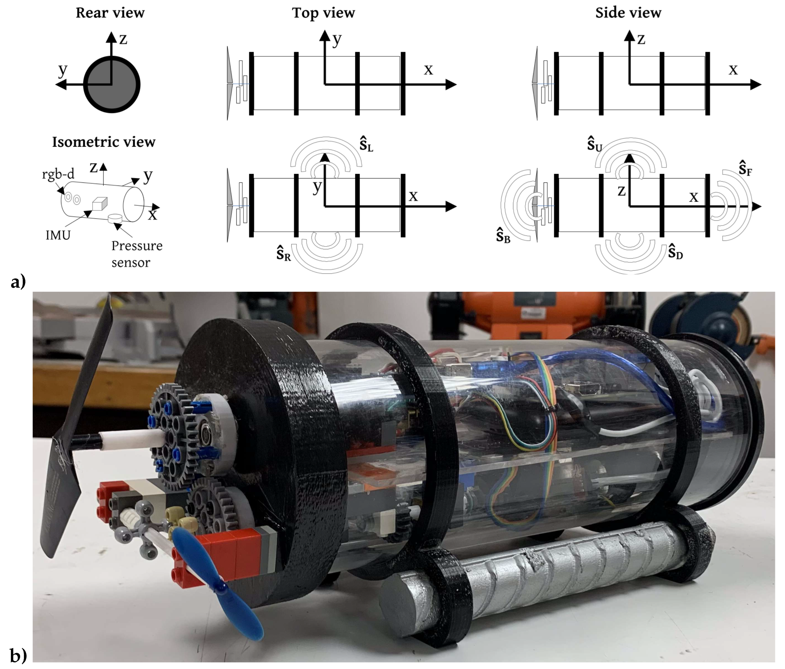
Figure 2.
Self-contained robotic submarine. a) Multi-view prototype. b) Modular system architecture.
Figure 2.
Self-contained robotic submarine. a) Multi-view prototype. b) Modular system architecture.
| µC |
| 64 bit |
| 4-Core |
| 1 GPU |
| Actuators control |
| slave System |
| Steer |
| Encoder |
| Thrust |
| Encoder |
| IMU |
| 6-Axis |
| Pressure |
| Sensor |
| Ballast |
| Encoder |
| Visual |
| Sensor |
| RGB |
| Steer |
| Propeller |
| Thrust |
| Propeller |
| Ballast |
| hydraulic |
| piston |
| Wi-fi |
| Module |
| Battery |
| Power Bank |
Figure 3.
Motors behavior model. a) Propulsion/steer motor speed () vs PWM digital word ().
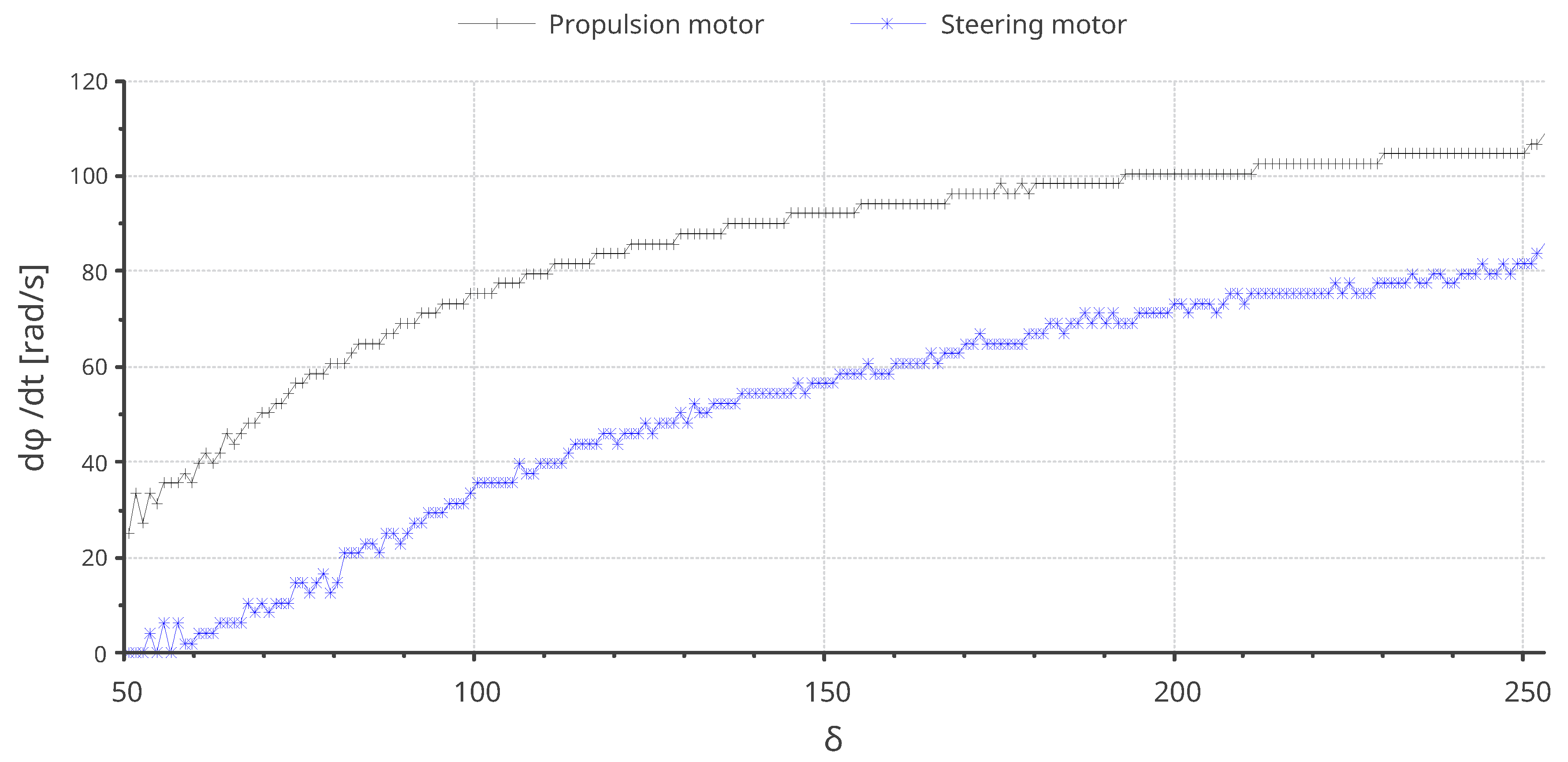
Figure 4.
Simplified planar representation of the robot’s state process Markov chain.
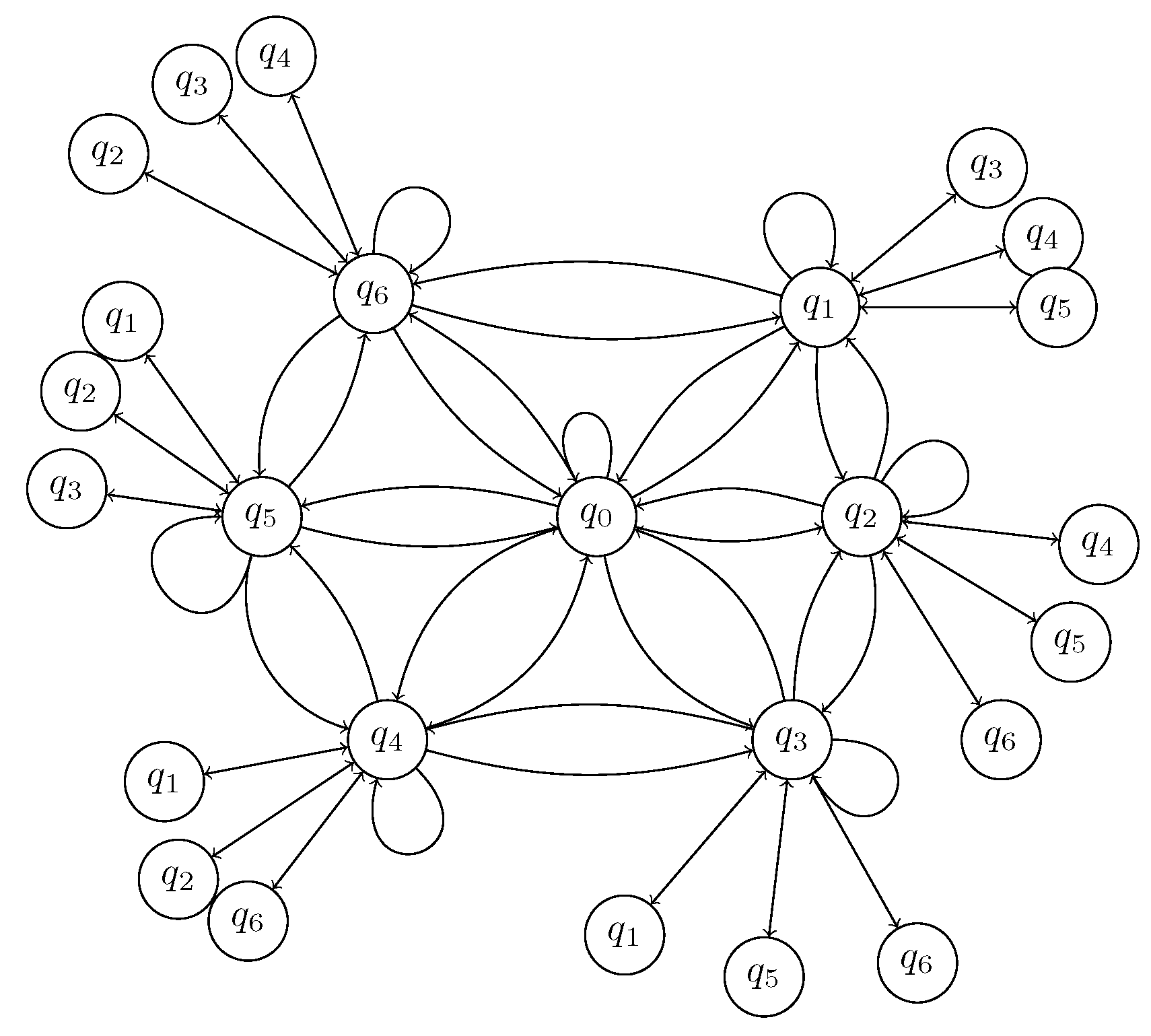
Figure 5.
Markov chain illustrating state transitions involved in upward collision while moving both forward and upward.
Figure 5.
Markov chain illustrating state transitions involved in upward collision while moving both forward and upward.
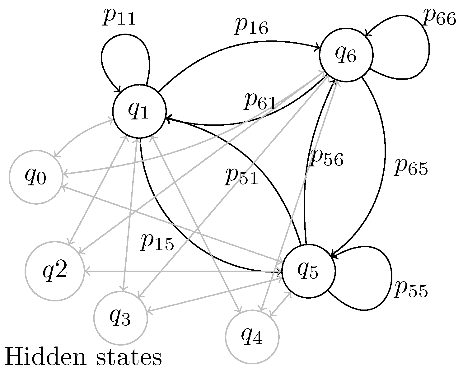
Figure 6.
Markov chain illustrating state transitions primarily affected to prevent simultaneous downward and rightward movements.
Figure 6.
Markov chain illustrating state transitions primarily affected to prevent simultaneous downward and rightward movements.
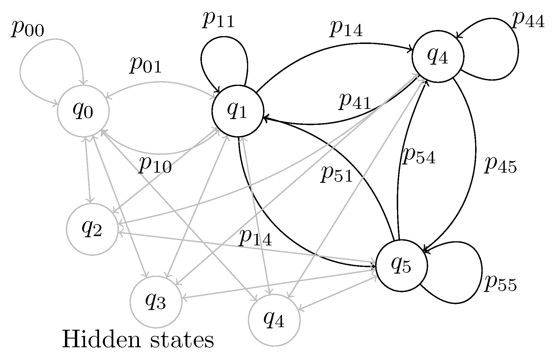
Figure 7.
Robot’s input fuzzy sets. a) Action task (HMC’s output state). b) Robot’s thrusting velocity . c) Robot’s underwater depth h.
Figure 7.
Robot’s input fuzzy sets. a) Action task (HMC’s output state). b) Robot’s thrusting velocity . c) Robot’s underwater depth h.
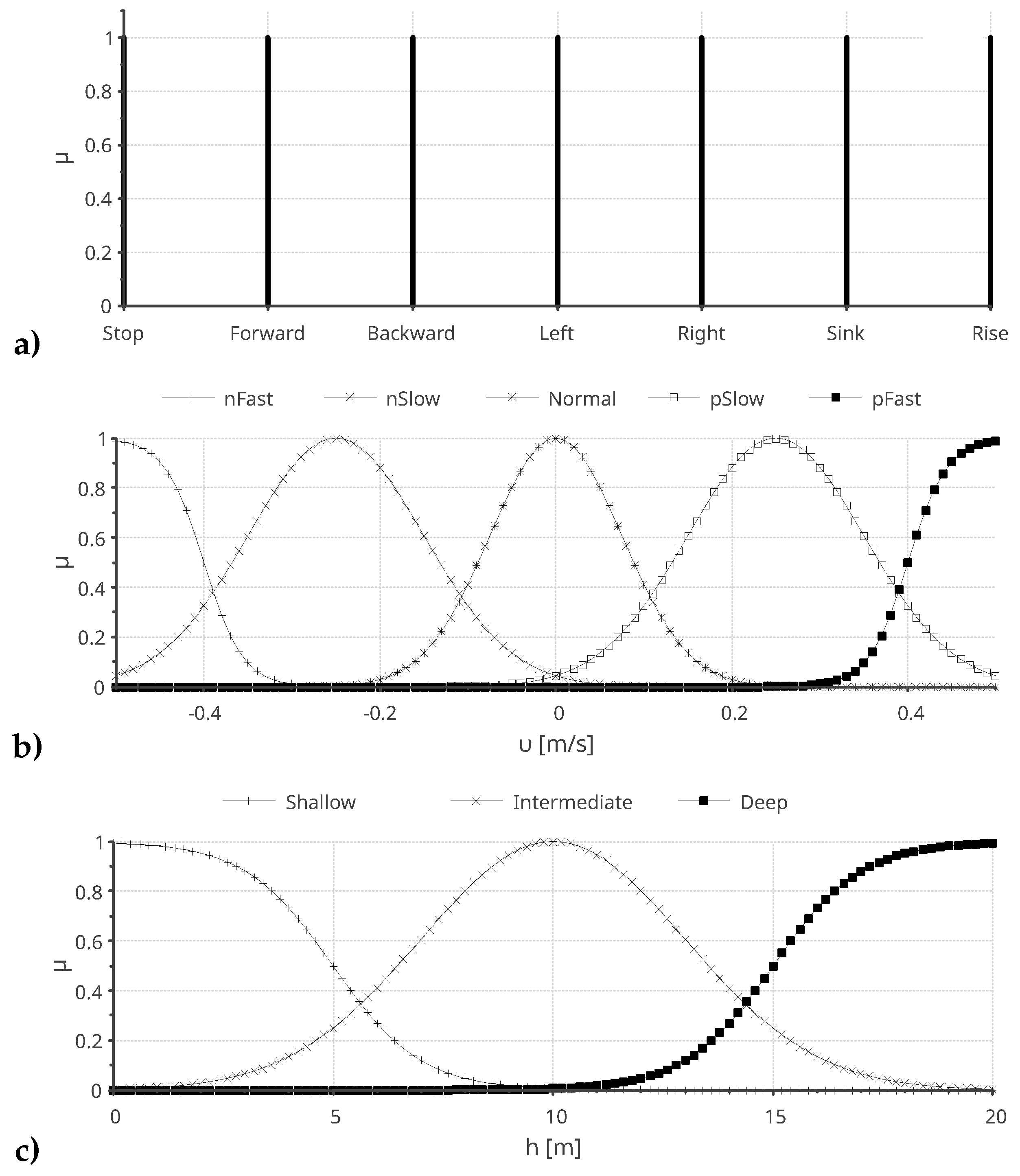
Figure 8.
Additional robot’s input fuzzy sets. a) Robot’s yaw velocity . b) Robot’s pitch velocity .
Figure 8.
Additional robot’s input fuzzy sets. a) Robot’s yaw velocity . b) Robot’s pitch velocity .
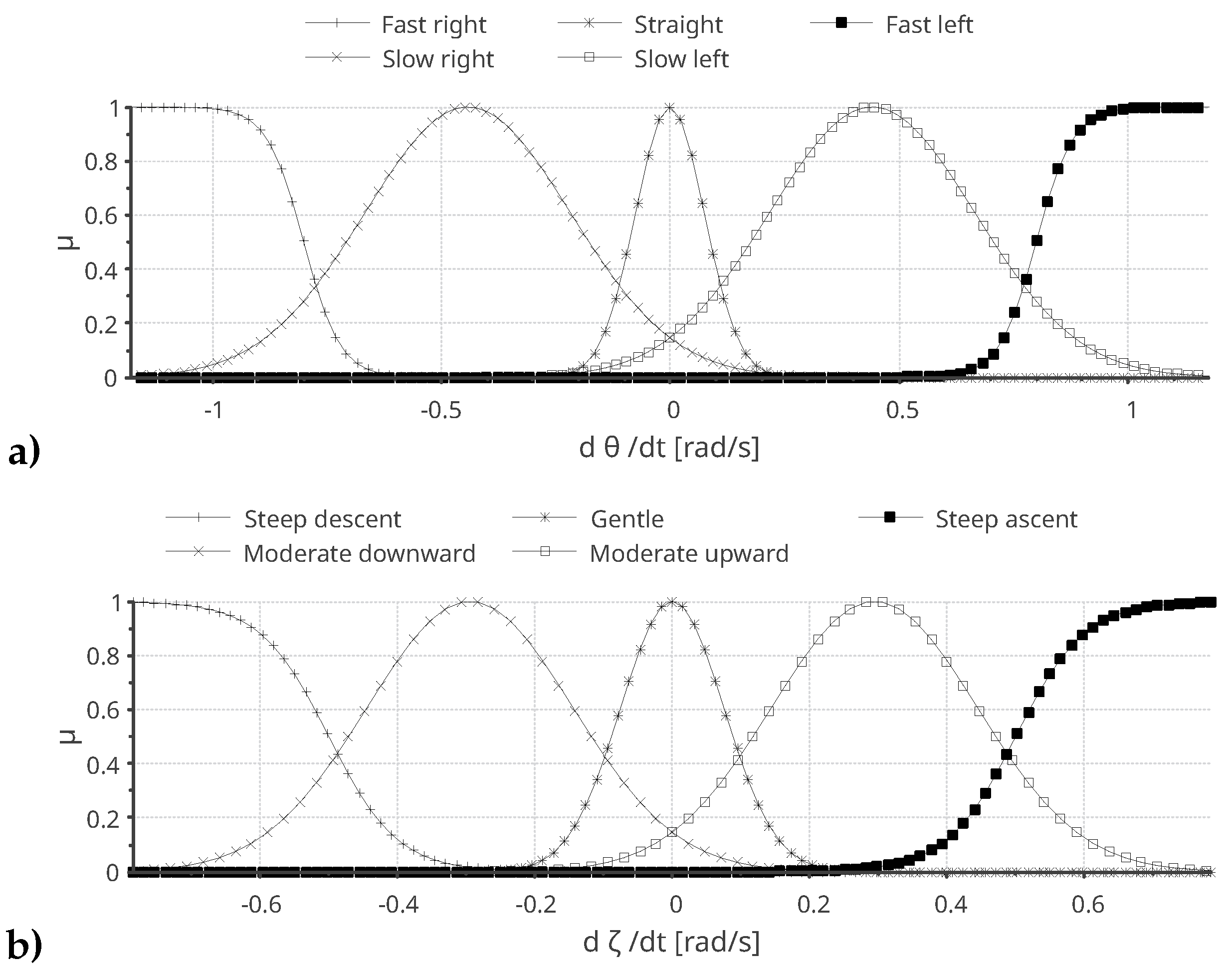
Figure 9.
Output fuzzy sets for the rotary actuators: thrust (), steer () and ballast ().
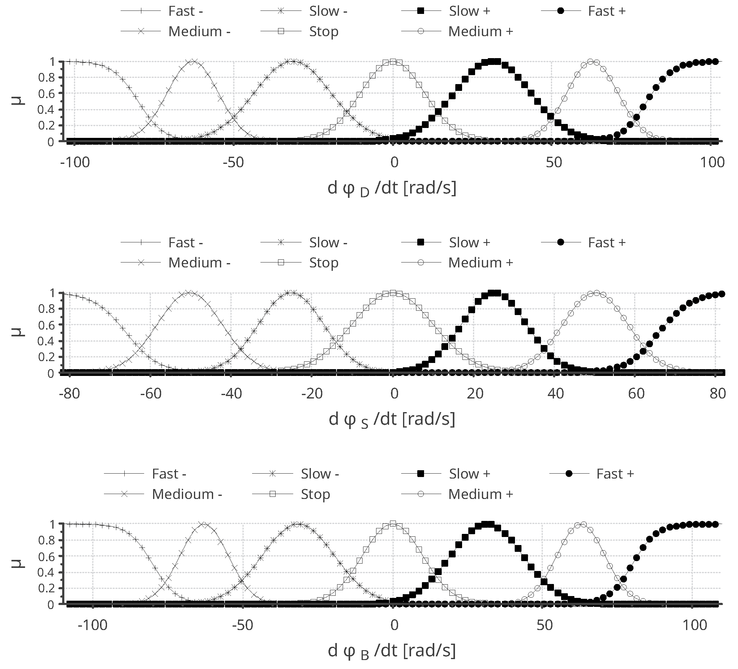
Figure 10.
Underwater robot’s inner elements.
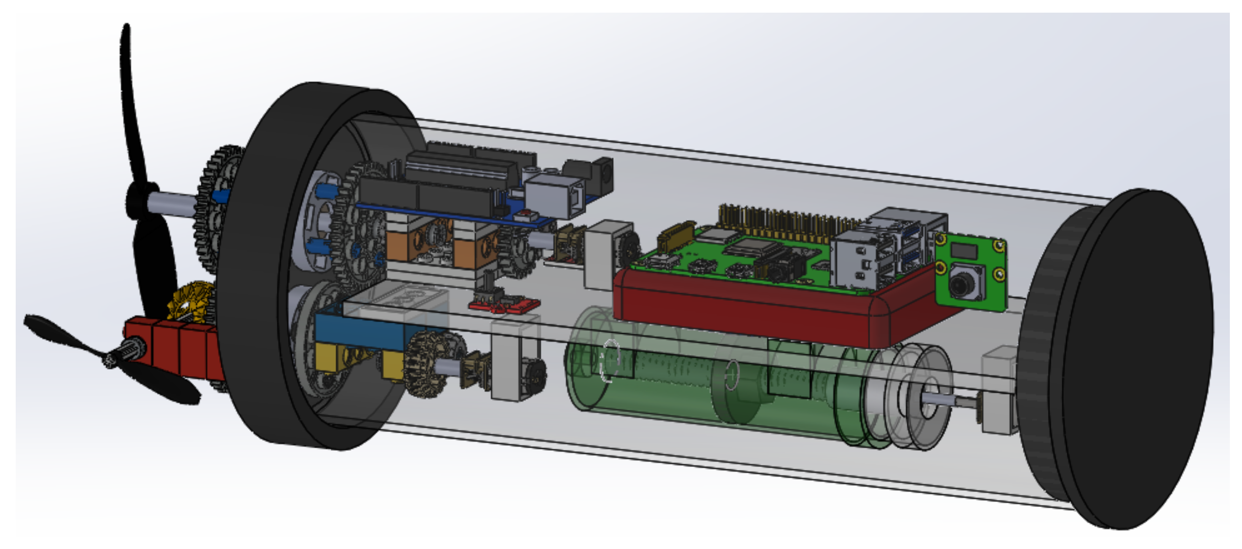
Figure 11.
Vertical movement ballasting experiment: (a) Descending phase; (b) Ascending phase.

Figure 12.
Experiment of the robot’s ballast system, demonstrating submersion to a depth of and subsequent resurfacing.
Figure 12.
Experiment of the robot’s ballast system, demonstrating submersion to a depth of and subsequent resurfacing.
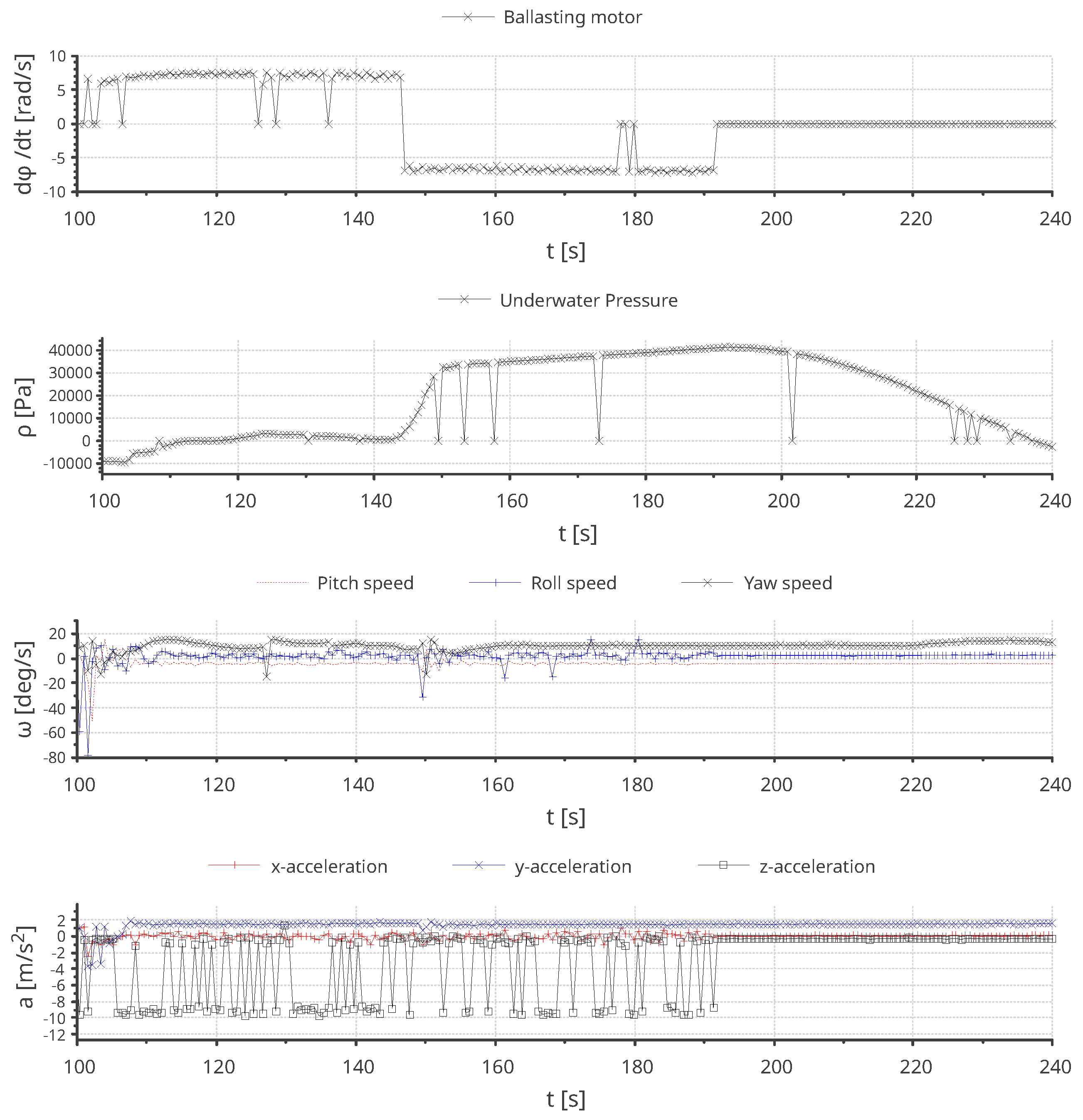

Table 1.
Markov’s elements description. The observation probability indicates likelihood of collision. means transition probability from any state to (stop).
Table 1.
Markov’s elements description. The observation probability indicates likelihood of collision. means transition probability from any state to (stop).
| Current | State | Activated | Observation | States | Transition |
|---|---|---|---|---|---|
| state | meaning | sensor | likelihood | Probability | probability |
| stop | all sensors | ||||
| forward | back-side sensor | ||||
| backward | front-side sensor | ||||
| left-turn | right-side sensor | ||||
| right-turn | left-side sensor | ||||
| sink | up-side sensor | ||||
| rise | down-side sensor |
Disclaimer/Publisher’s Note: The statements, opinions and data contained in all publications are solely those of the individual author(s) and contributor(s) and not of MDPI and/or the editor(s). MDPI and/or the editor(s) disclaim responsibility for any injury to people or property resulting from any ideas, methods, instructions or products referred to in the content. |
© 2025 by the authors. Licensee MDPI, Basel, Switzerland. This article is an open access article distributed under the terms and conditions of the Creative Commons Attribution (CC BY) license (http://creativecommons.org/licenses/by/4.0/).
Copyright: This open access article is published under a Creative Commons CC BY 4.0 license, which permit the free download, distribution, and reuse, provided that the author and preprint are cited in any reuse.


