
Submitted:
16 January 2025
Posted:
17 January 2025
You are already at the latest version
Abstract
Cardiac MRI images are vital in diagnosing a range of heart diseases, yet standard so-lutions frequently struggle with inadequate region delineation, confusion among simi-lar pathologies, and opaque decision-making processes. In this work, we aim to resolve these problems by introducing dedicated methods for careful region extraction, spe-cialized classification, and metric-based interpretation. Our approach notably im-proves segmentation, achieving Dice coefficients of 0.974 for the left ventricle and 0.947 for the right ventricle—outperforming prior baselines. Classification results reach a 97% overall accuracy, substantially higher than reference architectures that only attained 72–84%. Furthermore, clinical relevance is enhanced through a struc-tured output that pinpoints key anatomical and functional indicators. These findings suggest a reliable pipeline that refines MRI analysis and facilitates healthcare profes-sionals making more informed decisions in real-world medical settings.
Keywords:
cardiac MRI
; heart pathology
; explainable artificial intelligence
; explainable deep learning
; segmentation
; classification
; interpretation
1. Introduction
Over recent years, artificial intelligence (AI) methods in medical diagnostics have enabled the processing of complex medical images, detecting abnormalities, and suggesting preliminary diagnoses, thereby assisting physicians in making informed decisions [1,2]. Such technologies can significantly increase the efficiency of diagnostic processes by reducing dependence on the human factor and providing more standardized approaches to data analysis [3].
Cardiovascular diseases (CVDs) are the leading cause of death worldwide, claiming approximately 17.9 million lives each year [4]. Given the considerable impact of CVDs on public health, reliable methods for detecting cardiac pathologies are crucial for reducing morbidity rates. Cardiac magnetic resonance imaging (MRI) is critical in diagnosing and treating heart and surrounding tissue diseases. MRI of the heart allows for accurate assessment of anatomy, ventricular function, myocardial viability, the presence of myocardial inflammation, or occlusions in blood vessels. It is a primary noninvasive examination method that offers high resolution and specificity compared to other imaging techniques, such as computed tomography (CT) and ultrasound [5]. MRI is often called the gold standard due to its accuracy, reliability, and specificity [6].
Nowadays, cardiac MRIs employ standardized protocols to generate images for assessing left ventricular and right ventricular structures and functions, as well as comprehensive tissue characterization [7]. Despite these standardizations, the intricate cardiac anatomy, organ shape and size variability, and various image artifacts present significant challenges. Artifacts can result from patient movement, metal implants, or specific technical equipment settings. For example, motion artifacts, commonly caused by inconsistent heartbeats and breathing during scanning, necessitate specialized techniques to minimize their impact and enhance image quality [8]. These complexities render MRI scan analysis highly labor-intensive and resource-demanding.
Beyond technical challenges, the accuracy and objectivity of MRI interpretation are significantly influenced by human factors and cognitive biases. Physicians may experience confirmation or recency biases, leading to potential misdiagnoses or inappropriate treatments. Unconscious biases, including those related to race or gender, can also affect the quality of medical care, resulting in unequal access to healthcare services and disparate treatment outcomes among different patient groups [9,10]. Additionally, variability in physicians’ interpretations of the same clinical data complicates standardization and impairs diagnostic accuracy.
The “black box” problem inherent in AI systems, particularly those based on deep learning (DL) models, exacerbates these challenges. While AI can effectively process input data and generate outputs, the decision-making processes remain nontransparent due to the complexity of thousands of interacting parameters [11]. This omission undermines trust in AI systems, limits their applicability in critical fields like medicine, and heightens the risks associated with incorrect or unjustified conclusions.
To address the black box issue, existing approaches focus on enhancing AI transparency through interpretation and visualization methods [12]. Techniques such as heatmaps to highlight significant image regions and visualization of feature importance enable a deeper understanding of how AI systems make decisions. These tools facilitate the validation of AI results and bolster user trust, which is crucial in high-stakes environments.
Automating diagnosis and treatment prescription using AI is theoretically feasible by accounting for all physiological indicators and individual patient features (e.g., body structure, allergies, drug responses). However, the practical implementation faces substantial challenges, including the immense scale, time, and financial costs required to organize and label such extensive datasets [13]. Moreover, specific subjective indicators, such as patient-reported well-being or pain thresholds, necessitate physician evaluation during consultations, as AI cannot easily quantify them. Consequently, patients with identical diagnoses and physiological indicators may receive different treatments based on individual physician assessments, which are sometimes justified.
Modern medical and computer science strives to minimize subjectivity in treatment. Integrating objective data and AI algorithms reduces the likelihood of biases, promoting a more standardized approach. Conversely, physicians’ subjective assessments allow for the consideration of unique aspects of patients that are difficult to formalize. Balancing objective AI-driven indicators with subjective clinical judgments can optimize diagnostic and treatment processes, ensuring both accuracy and individualized patient care.
Hence, it is necessary to balance objective indicators and subjective factors when making medical decisions. Objective data and AI algorithms can reduce the likelihood of biases by providing a more standardized approach. In contrast, a physician’s subjective assessment allows for considering unique aspects of patient well-being that are difficult to formalize. This balance may help optimize the diagnostic and treatment process, making it both accurate and individualized.
The main contributions of this paper are as follows:
- A multi-stage method is proposed for segmenting the heart region into the right ventricle (RV), left ventricle (LV), and myocardium, differing from existing approaches by combining the U-Net and ResNet DL models for localizing and segmenting these cardiac structures, followed by Gaussian smoothing for contour refinement and artifact reduction. This method significantly improves segmentation accuracy, with the Dice coefficient reaching 0.974 for LV segmentation and 0.947 for RV segmentation.
- A cascade classification method for pathologies—dilated cardiomyopathy (DCM), hypertrophic cardiomyopathy (HCM), myocardial infarction with altered left ventricular ejection fraction (MINF), and abnormal right ventricle (ARV)—on MRI scans is proposed. This method differs from existing ones by applying a cascade of DL models to segmented MRI scans, achieving higher disease classification accuracy for the four pathologies under consideration: 0.96, 1.00, 1.00, and 0.90, respectively, and an overall classification accuracy of 0.972.
- A method for interpreting the decisions obtained by DL is proposed, differing from existing approaches by explaining the features used in medical practice, which makes the decisions transparent and comprehensible.
The paper is structured as follows: Section 2 reviews contemporary approaches to segmenting, classifying, and interpreting cardiac MRI data using DL. Section 3 describes the three proposed methods: a multi-stage segmentation technique integrating U-Net and ResNet architectures, a cascade classification procedure tailored for DCM, HCM, MINF, ARV, and NOR, and an interpretation method that highlights clinical features such as myocardial thickness and ejection fraction. Section 4 presents the results of the proposed methods, comparing them to state-of-the-art techniques. Section 5 draws final conclusions, addresses limitations, and outlines possible future research directions.
2. Related Works
Below is an analysis of related works concerning (i) methods for segmenting cardiac MRIs, (ii) methods for classifying pathologies in MRI scans, and (iii) methods for interpreting the decisions produced by DL models.
2.1. Segmentation of Cardiac MRIs
Traditional segmentation techniques, including edge detection-based segmentation [14], threshold-based segmentation [15], and region-based image segmentation [16], are valued for their low computational complexity and high processing speed. However, these methods fall short in accuracy and quality compared to contemporary DL-based approaches [17].
DL methods, particularly convolutional neural networks (CNNs), have advanced medical image segmentation by identifying complex patterns within data [18]. Architectures like U-Net [19] and SegNet [20] have demonstrated superior accuracy even with limited datasets. These models excel because they can learn hierarchical features and adapt through retraining with new data, improving over time. Nonetheless, their advantages come with significant drawbacks, including high computational resource requirements and the necessity for extensive labeled training data [21]. Additionally, the “black box” nature of DL models raises trust issues, prompting interest in “human-in-the-loop” [22] and “human-centric” [23] approaches to enhance transparency and reliability.
Hybrid segmentation techniques that integrate classical and DL approaches are gaining traction. For instance, combining CNN-based preprocessing with active contour models leverages the strengths of both methods, achieving precise boundary detection. Similarly, ensemble learning methods incorporating multiple DL models can enhance segmentation accuracy by addressing different aspects of the image-processing task. These hybrid strategies, while effective, demand more significant computational resources and complex model tuning. Specialized models tailored to specific cardiac regions have shown improved accuracy by focusing on unique anatomical features [24].
Multimodal approaches that utilize multiple imaging modalities, such as combining CT and MRI data, aim to improve segmentation accuracy by integrating complementary information. However, these methods face significant challenges in dataset creation and integration, as aligning and harmonizing data from different sources is complex [25,26]. For example, Hu et al. [27] developed a deeply supervised network combined with a 3D Active Shape Model to reduce manual initialization efforts, achieving high accuracy but limited by substantial computational demands and lack of validation across varied imaging protocols. Similarly, da Silva et al. [28] designed a cardiac segmentation technique for short-axis MRI that employs six fully CNNs. Their framework comprises one CNN dedicated to the region of interest (ROI) extraction, three CNNs for the initial segmentation phase, and two additional CNNs for the reconstruction stage. Despite this comprehensive approach, their methodology exhibited reduced performance on end-systolic (ES) slices compared to end-diastolic (ED) slices in most cases.
Self-supervised and semi-supervised learning methods have emerged as promising solutions to the scarcity of labeled medical data. Contrastive learning techniques [29,30] have shown success by learning representations by distinguishing similar and dissimilar data samples. Recent studies [31,32] have developed efficient self-supervised learning frameworks specifically for medical image segmentation, enabling models to learn robust features without extensive labeled datasets. These approaches significantly reduce the reliance on manual annotations, making them highly valuable for medical imaging applications where labeled data is limited.
Recent research has explored the integration of segmentation and classification tasks to streamline the diagnostic workflow. For instance, Zheng et al. [33] employed semi-supervised learning for explainable DL to classify MRI scans yet encountered challenges with motion artifacts, highlighting the need for robust models to handle real-world imaging variances. Ammar et al. [34] developed a combined segmentation-classification pipeline for diagnosing heart diseases, achieving enhanced accuracy but at the cost of increased training complexity. Bourfiss et al. [35] introduced a corrective framework to address segmentation errors, which required manual intervention and increased workflow complexity.
Overall, while self-supervised methods offer significant advancements in medical image segmentation, they are computationally expensive and require numerous training iterations. Training such models typically necessitates robust computing infrastructure, making them less accessible for widespread clinical use.
2.2. Classification of Cardiac MRIs
Traditional machine learning techniques, including support vector machines (SVM), decision trees, and ensemble methods like random forests, have been employed for medical image classification using handcrafted features such as textures and shapes. While these methods are suitable for more straightforward tasks, they are generally outperformed by DL models, especially when handling large and complex datasets [36].
CNN architectures, notably ResNet [37] and DenseNet [38], play a crucial role in medical image classification by automatically extracting intricate features from input data. DenseNet, in particular, has proven highly effective in tumor image classification by processing small patches from extensive digital pathological images [36]. These architectures facilitate the creation of highly accurate models capable of distinguishing subtle pathological differences.
Methodologies have been developed to enhance classification accuracy by integrating segmentation outputs with classification algorithms. For example, one approach [36] uses segmentation masks to extract time-series data on myocardial segment radius and thickness, constructing motion maps that inform a logistic regression model to classify five cardiac pathologies: DCM, HCM, MINF, ARV, and patients without cardiac disease (NOR). This method achieves high accuracy (95% training, 94% testing) while maintaining explainability and simplicity, crucial for clinical adoption.
Another study [39] focuses on disease classification using cine-MRI data through a combined segmentation and classification model. Utilizing a U-Net for segmentation, the model extracts both static and dynamic features from segmented regions, including ventricular volume and myocardial thickness. These handcrafted features are then used to train an ensemble of multilayer perceptrons (MLPs) and a random forest classifier, achieving segmentation Dice coefficients of 0.945 (LV), 0.911 (myocardium), and 0.923 (RV), along with classification accuracies of 94% (training) and 92% (testing). However, this model struggles to differentiate between similar pathologies like DCM and MINF.
The classification approach in [40] integrates DL and ensemble classifiers for automated heart disease diagnosis from cine-MRI. Using DenseNet-based CNNs for segmentation, the method extracts clinically relevant features such as ventricular volumes and myocardial mass. An ensemble of classifiers (SVMs, MLPs, etc.) then classifies five categories (ARV, HCM, MINF, DCM, NOR), achieving high Dice coefficients (0.96 LV, 0.95 RV, 0.89 myocardium) and a classification accuracy of 100%. However, the ensemble’s complexity and potential overfitting, particularly with smaller datasets, limit its practicality and ability to distinguish between similar pathologies without expert intervention.
2.3. Interpretation of DL Models
A significant challenge in adopting AI in clinical settings is the interpretability of DL models. Overcoming the “black box” nature of these models is essential for building trust among clinicians. Current studies emphasize the use of heatmaps and saliency maps to visualize important image regions, thereby enhancing physician confidence and improving diagnostic accuracy for MRI and other medical scans [41].
Research [42] highlights the expanding role of AI in cardiovascular diagnostics, noting improvements in accuracy and speed of image analysis, reduction of human errors, and minimized radiation exposure. These advancements underscore the potential of AI to rival expert clinicians while emphasizing the need for broader exploration across diverse cardiology applications. Guidelines outlined in [43] focus on evaluating trust in AI systems for medical imaging, emphasizing strategies to mitigate ethical and clinical risks. Ensuring alignment with clinical practices is vital for AI’s safe and effective deployment in diagnosing cardiac diseases.
The deep Taylor-CAV (D-TCAV) method discussed in [44] offers concept-based explanations for AI model decisions in cardiac image segmentation. By identifying key image regions that influence outcomes, such as uneven walls or chamber size differences, D-TCAV provides objective data that supports diagnostic analysis. This approach enhances transparency and reliability, reducing the risk of biased or arbitrary model decisions and fostering trust in AI-driven cardiology tools. It can be clearly observed that contemporary research underscores the importance of developing interpretable AI models to facilitate their integration into cardiology. Visualization and explanation tools are crucial for making AI outputs understandable to clinicians, thereby increasing the reliability and clinical accessibility of AI technologies for patient diagnosis and treatment.
In summary, related works demonstrate significant advancements in cardiac MRI segmentation and classification through DL models, while also addressing the need for interpretability and trust in AI systems. These developments highlight the potential of AI to enhance diagnostic accuracy and efficiency in cardiology, provided that challenges related to model transparency and ethical considerations are effectively managed.
2.4. Aim of the Study and Research Objectives
From the above analysis of related works, the main goal of this research is to improve the quality of cardiac MRI scan segmentation and classification and to enable the interpretation of DL-based decisions. This goal is pursued through the following steps:
- Develop a multi-stage segmentation method for dividing the heart region in MRI scans into the RV, LV and myocardium. This method combines U-Net and ResNet models for localizing and segmenting cardiac structures, followed by Gaussian smoothing for contour refinement and artifact reduction.
- Develop a cascade classification method for pathologies—DCM, HCM, MINF, and ARV—in MRIs, to more accurately categorize heart pathologies using segmented MRI data.
- Develop a method for interpreting DL decisions based on clinical features commonly used in medical practice.
3. Methods and Materials
Recall that this study focuses on detecting the following cardiac pathologies via MRI scans: DCM, HCM, MINF, and ARV. These particular pathologies were chosen due to their high prevalence and clinical significance. They are among the most common heart diseases [45,46], characterized by a range of morphological and functional changes that MRI can detect. Publicly available, high-quality dataset titled Automated Cardiac Diagnosis Challenge (ACDC) [47] includes annotated MRI scans for each condition. While the four pathologies cover major categories of cardiac disease—cardiomyopathies, inflammatory conditions, and arrhythmogenic states—they do not represent the full spectrum detectable by MRI. Ischemic diseases, restrictive cardiomyopathy, sarcoidosis, and congenital disabilities, for instance, are excluded due to their lower prevalence and a lack of sufficiently high-quality datasets for research.
In this study, the proposed approach to explainable AI-based detection of the aforementioned cardiac pathologies in MRI scans is decomposed into separate tasks, each solved by corresponding methods (Figure 1):
- A multi-stage method for MRI scan segmentation.
- A cascade classification method for pathologies.
- A method for interpreting DL decisions.
This decomposition is motivated by the following considerations.
- Instead of analyzing the entire cardiac MRI scan, focus on the localized and segmented areas that are relevant for analysis (RV, LV, and myocardium). This enables the DL model to concentrate on essential regions rather than extraneous information. Isolating this function as a separate task allows for selecting specialized DL models best suited for such preprocessing.
- Medical datasets for classifier training often have limited sample sizes, making it challenging to achieve sufficient model generalization for multiple classes. Class confusion is common. Many approaches have been proposed to address this issue, including data augmentation. Using a cascade of separate binary classifiers for aggregated classes allows the model to increase the number of samples per aggregated class and focus on specific features of two aggregated classes simultaneously, leading to higher classification accuracy.
- In the medical domain, the problem of interpretability of AI models is particularly critical. Addressing this issue is essential to overcome the “black box” effect, which undermines trust in clinical AI outcomes. This study proposes presenting DL-based results in a physician-friendly format through clinically familiar features.
The following sections provide a more detailed description of each method proposed to solve these decomposed tasks.
3.1. Method of Multi-Stage Cardiac MRI Segmentation
At first, the idea of the method was initially approbated at the Informatics & Data-Driven Medicine (IDDM-2023) conference [48].
In this study, an original dataset, extracted from the ACDC dataset and denoted contains pairs of MRI scans and physician-created masks covering three cardiac regions of interest—(i) LV, (ii) RV, and (iii) Mo:
where is the cardiac MRI scan, is its corresponding mask, and N is the total number of pairs.
Existing solutions train a single DL model on per formula (1) to detect all three regions at once. However, studies [24,25] suggest specialized DL models can yield more precise results. Accordingly, this research proposes:
- Prelocalizing (detecting) LV, RV, and myocardium areas on the MRI scan.
- Using three separate masks instead of a single multistructure one.
We hypothesize that these changes improve segmentation accuracy. Therefore, we introduce six DL models:
- , , : localize LV, RV, and myocardium, respectively.
- , , : refine the contours (masks) for each of those regions.
For , , , we utilize U-Net with a ResNet-50 encoder; for , , the same approach but with ResNet-34. In both cases, training requires adapted datasets derived from .
A second dataset is defined to train , , :
where is the cropped cardiac MRI, while are its three cropped masks.
All images in dataset per formula (2) are resized to a uniform resolution. Original masks from are decomposed into separate LV, RV, and myocardium masks.
For , , , three further datasets , , are formed:
Each dataset formalized by formulas (3)–(5) localizes and centers images/masks around one structure, adding a 15% margin. After segmentation, images must revert to original dimensions for final validation, possibly causing detail loss. To address this, Gaussian smoothing is utilized as suggested in our previous work [48]—balancing quality and computational cost better than other filters. The parameter is automatically chosen via linear regression, fitting optimal to each image size.
Thus, the task of obtaining DL models for subsequent segmentation of regions of interest in an MRI scan is presented through the following steps of the method (Figure 2).
Next, we describe in detail the steps for creating DL models that are used for MRI scan segmentation.
The input data here is a subset of [47], which contains pairs of MRI scans and corresponding masks with regions of the LV, RV, and LV myocardium.
In Step 1, DL models are trained to localize the regions of the LV, RV, and myocardium. Specifically, in Step 1.1, a new dataset is prepared, which contains three masks instead of one: for the LV, RV, and myocardium. This involves the following substeps:
Step 1.1.1: Resizing all input images and masks to a uniform size.
Step 1.1.2: Decomposing the original mask into separate masks for the LV, RV, and myocardium.
Thus, the new dataset contains rows containing an MRI scan and three masks.
Next, in Step 1.2, using dataset , three DL models are trained to detect the regions of interest as follows:
Step 1.2.1: Training DL model to detect the LV region.
Step 1.2.2: Training DL model to detect the RV region.
Step 1.2.3: Training DL model to detect the myocardium region.
In Step 2, DL models are trained to generate masks based on the detected regions of interest. In Step 2.1, new datasets , , and are prepared by modifying dataset , specifically by cropping the original MRI scans and masks according to the regions of interest.
Subsequently, in Step 2.2, using datasets , , and , three DL models are trained to delineate the contours of the LV, RV, and myocardium:
Step 2.2.1: Training DL model to delineate the LV contours using dataset .
Step 2.2.2: Training DL model to delineate the RV contours using dataset .
Step 2.2.3: Training DL model to delineate the myocardium contours using dataset .
The output data consists of the trained DL models , , , , , .
The task of segmenting an arbitrary MRI scan into regions of the LV, RV, and myocardium using the trained DL models , , , , , and is presented through the following steps of the method (Figure 3).
Next, we describe the steps for segmenting an MRI scan into regions of the LV, RV, and myocardium. The input data consists of an MRI scan and the DL models , , , , , and .
Step 1: Determine the locations of the LV, RV, and myocardium regions:
Step 1.1: Using DL model , determine the location of the LV.
Step 1.2: Using DL model , determine the location of the RV.
Step 1.3: Using DL model , determine the location of the myocardium.
Step 2: Generate masks for the LV, RV, and myocardium:
Step 2.1: Using DL model , generate the mask for the LV.
Step 2.2: Using DL model , generate the mask for the RV.
Step 2.3: Using DL model , generate the mask for the myocardium.
Step 3: Perform postprocessing of the obtained masks:
Step 3.1: Smoothing the masks.
Step 3.2: Combining the three individual masks into a single comprehensive mask.
Step 3.3: Mapping the combined mask to match the size of the input image.
The output of the method is a segmented arbitrary MRI heart image into regions of the LV, RV, and myocardium.
Thus, the process of constructing DL models includes data preparation and training models for localization and mask generation of regions of interest using modified datasets. Separate models are trained for localizing and delineating the contours of the LV, RV, and myocardium. In total, six DL models were trained.
MRI scan segmentation is performed sequentially: first, the models determine the locations of the LV, RV, and the myocardium regions, after which the corresponding masks are generated. The final step is postprocessing the masks, which includes smoothing, combining, and adapting them to the size of the input image. The result is a segmented MRI heart image.
3.2. Method of Cardiac MRIs Cascade Classification
The idea of this method was originally presented at the Information Technology and Implementation (IT&I-2024) conference [49].
This study focuses on four pathologies in MRI scans: DCM, HCM, MINF, ARV, including normal state denoted NOR. The proposed method includes the following:
- Accounting for anatomic heart parameters via certain modifications of an input MRI.
- Using both diastolic and systolic MRI phases.
- A cascade classification model.
- A custom DL architecture.
Heart pathologies often depend on tissue density, chamber volumes, and myocardial thickness over time. We use segmentation masks obtained by the multi-stage approach to capture geometry and texture. Each structure (LV, RV, and myocardium) is placed in a separate RGB channel, preserving texture in addition to geometry.
Therefore, based on the above considerations, the following decomposition of the input MRI scan is proposed:
where are systolic short-axis slices, and are diastolic slices.
Images denoted by Formula (7) are cropped into bounding boxes that contain all relevant segments. Figure 4 shows the images that are fed to the DL model.
Based on the representation defined by Formula (6), a dataset is constructed:
where denotes the pathology class (1—ARV, 2—HCM, 3—MINF, 4—DCM, 5—NOR).
Dataset is derived from the ACDC dataset, containing systolic and diastolic images for 150 patients in five groups. Some have fewer than 21 short-axis slices; thus, image augmentation is performed by duplicating adjacent slices.
A cascade classification model is proposed to mitigate class confusion in smaller datasets. We define four binary classifiers (, , , ):
- —class a—aggregation of classes 1 and 5, class b—aggregation of classes 2, 3, and 4. This model separates all LV pathologies from ARV/NOR—LV pathologies vs. ARV/NOR.
- —class a—class 1, class b—class 5. is aimed to distinguish ARV from NOR, i.e., splits ARV vs. NOR.
- —class a—class 2, class b—aggregation of classes 3 and 4. It distinguishes ARV from NOR, i.e., splits ARV vs. NOR.
- —class a—class 4, class b—class 3. This model differentiates MINF from DCM.
The structure of the proposed cascade classification is shown in Figure 5.
Each model (, , , ) uses a CNN adapted to binary classification, with Adam optimizer and categorical cross entropy as the loss. Adam adaptively adjusts learning rates while cross entropy measures the discrepancy between real labels and predicted probabilities. Early stopping is applied to avoid overfitting, and class proportions are maintained in training and validation splits.
The proposed method consists of two processes: i) training models , , , and and ii) classifying pathology using an arbitrary cardiac MRI. The overall scheme of this process is illustrated in Figure 6.
Below, the main steps of the proposed method are described in detail.
The input data consists of images from the ACDC dataset [47], modified as described above, which contain images for each patient during the diastolic and systolic phases of the cardiac cycle.
Step 1: Preparation of MRI scans.
Step 1.1: All MRI scans are cropped to retain only the area with the necessary segments (identified using the first method) and resized to a uniform size.
Step 1.2: Mask data and images are combined (each heart segment corresponding to the mask is presented in a separate channel).
Step 1.3: Image and mask data are augmented to obtain an equal number of elements for each patient.
Step 1.4: Masks and images from the diastolic and systolic phases of the cardiac cycle are combined.
Step 2: Training a Cascade of Four Classifiers.
Each classifier is trained separately using the same approach. The training process begins with creating and compiling the model.
Step 2.1: Training the classifier model .
Step 2.2: Training the classifier model .
Step 2.3: Training the classifier model .
Step 2.4: Training the classifier model .
The output of this method is a trained cascade of classifiers consisting of models , , and .
Next, we consider the process of classifying pathology using an arbitrary cardiac MRI. Figure 7 illustrates the scheme of this process.
The main steps of the method of cardiac MRIs cascade classification are presented below.
The input data consists of a set of cardiac MRI scans of an arbitrary patient containing images during the diastolic and systolic phases of the cardiac cycle.
Step 1: Preparation of MRI scans.
Step 1.1: All MRI scans are cropped to retain only the area with the necessary segments (identified using the first method) and resized to a uniform size.
Step 1.2: All patient images are segmented using the multi-stage MRI scan segmentation method described in section 3.1.
Step 1.3: Image and mask data are combined (each heart segment corresponding to the mask is presented in a separate channel).
Step 1.4: Image and mask data are augmented to obtain the number of elements corresponding to the trained model (21 images).
Step 1.5: Masks and images from the diastolic and systolic phases of the cardiac cycle are combined.
Step 2: Application of the Cascade of Classifiers to Determine Pathologies.
Step 2.1: Application of classifier .
Step 2.2: If the result from corresponds to class a, apply classifier .
Step 2.3: If the result from corresponds to class b, apply classifier .
Step 2.4: If the result from corresponds to class a, apply classifier .
The output of the method is the determination of one of the following pathologies: ARV, HCM, MINF, DCM, or NOR.
3.3. Method of Interpreting Obtained Decisions based on Cardial MRI
3.3.1. Features Indicating Heart Diseases
To elucidate the decisions made by DL models, it is essential to transform DL architecture outputs into clinically relevant features used by physicians for diagnosing heart diseases. The following key feature groups are formulated based on the heart diseases addressed in this study.
Group 1: Ventricular volumes. Heart volume indicators assess the function of the LV and RV). The ratio of LV volume to RV volume at the ES evaluates ventricular balance during contraction. LV volumes at ES and ED indicate contractile ability and blood capacity, respectively. Similarly, RV volumes help identify dysfunctions; for instance, increased RV volume at the ED may signify ARV, while decreased LV volume at the ES may suggest HCM as investigated in [50,51].
Group 2: Ejection fraction. Ejection fraction measures the efficiency of blood ejection by the ventricles. LV ejection fraction reflects the proportion of blood pumped out during each contraction, which is crucial for diagnosing DCM, where it is typically reduced. RV ejection fraction indicates the pumping efficiency of the RV, which is crucial for diagnosing ARV [51].
Group 3: Volume-to-mass ratios. This group assesses the ratio of heart volumes to myocardial mass, aiding in detecting pathological changes. An increased myocardial mass relative to LV volume may indicate hypertrophic changes, while a decreased ratio suggests dilative processes as stated in [33,51].
Group 4: Thickness and variability of the myocardium walls. Myocardial wall thickness and its variability are vital for classifying heart diseases. Increased wall thickness during diastole may indicate HCM, whereas decreased thickness suggests dilative processes. Variability in wall thickness during the cardiac cycle assesses the uniformity of myocardial contractions, with high variability pointing to uneven contractions characteristic of specific cardiomyopathies like HCM, following [50].
3.3.2. Interpretation and Visualization Model
Below is the information model for interpreting decisions made by deep learning models using transformations :
where d indicates the pathology (1—DCM, 2—HCM, 3—MINF, 4—ARV, 5—NOR), I is the segmented MRI scan, and is a set of features for pathology d defined as follows:
with ‘name’ as the feature name and ‘’ as the presentation mode: —17-segment myocardium model, —circular chart, and —numeric representation.
Below are the measures for each pathology from the set per formula (10), along with recommended visualization methods.
- d = 1—DCM: = (LV ED volume, ); = (LV ES volume, ); = (LV ejection fraction, ); = (myocardial mass at ED, ); = (ratio of myocardial mass to LV ED volume, ); = (maximum average myocardial wall thickness in ED, ).
- d = 2—HCM: = (LV ES volume, ); = (LV ejection fraction, ); = (ratio of myocardial mass to LV ES volume, ); = (maximum average myocardial wall thickness in ED, ); = (mean standard deviation of wall thickness in ES, ); = (mean standard deviation of wall thickness in ED, ).
- d = 3—MYOC: = (LV ED volume, ); = (LV ejection fraction, ); = (myocardial mass at (ED), ); = (maximum average myocardial wall thickness in ED), ); = (mean standard deviation of wall thickness in ED, ).
- d = 4—ARV: = (RV ED volume, ); = (RV ejection fraction, ); = (ratio of LV to RV ED volumes, ); = (maximum average myocardial wall thickness in ES, ); = (mean standard deviation of wall thickness in ES,
- d = 5—NOR: = (LV ES volume, ); = (LV ED volume, ); = (ratio of LV to RV ED volumes, ); = (LV ejection fraction, ); = (maximum average myocardial wall thickness in ES, ).
Hence, volumes and ejection fraction are displayed numerically, ratios with circular charts, and wall thickness/variability using the 17-segment model. This layout helps clinicians grasp key cardiac metrics from a single image without comparing multiple MRI slices.
3.3.3. Main Steps of the Proposed Method
This section outlines the main steps of the method for interpreting results obtained through DL means. The primary goal of the method is to present key features in a format suitable for visualization and analysis, thereby ensuring transparency in the pathology classification process. The overall scheme of the result interpretation method is depicted in Figure 8. The steps, input, and output information are described below.
The input data for the method consists of a segmented MRI scan (using the multi-stage segmentation method presented in subsection 3.1) and its classification result.
Step 1: Obtaining feature values. The values of features for pathology d are determined from the input image. This provides a numerical basis for further analysis.
Step 2: Presentation of obtained features. The features are presented to the end user separately by types for the corresponding pathologies.
The output of the method is the input segmented and classified MRI scan along with the visualized type features.
Thus, the main steps of the decision interpretation method enhance the accessibility and comprehensibility of the obtained data for further analysis. Users, including physicians and researchers, can assess the classification results by calculating key features and visualizing them. This increases trust in the DL models and facilitates their practical use in diagnosing patients with heart pathologies.
3.4. Evaluation Approaches and Metrics
In this study, we utilized several essential metrics to assess the performance of our DL models in medical applications, covering both segmentation and multiclass classification tasks. Our findings are consistent with existing research on model evaluation in medical image analysis, as highlighted in Rainio et al. [52].
3.4.1. Experimental Models for Validating the Multi-Stage Segmentation Method
To objectively measure how each stage of the multi-stage segmentation method (see subsection 3.1) affects final segmentation quality, a series of experiments was performed with identical epochs, architectures, and data. Results were averaged over 10 training/testing cycles, and segmentation accuracy was assessed using the Dice coefficient, comparing predicted and expert masks.
To evaluate the combined impact of these steps, an arithmetic mean of Dice across all structures (LV, RV and myocardium) in both ES and ED phases was calculated. Six additional models were developed to test specific components:
- Base model : Trained without any optional preprocessing or postprocessing (only uniform resizing). It serves as a baseline for recognizing heart structures on the original ACDC dataset.
- Localization models and : localizes the heart region as a single binary mask, while segments LV, RV, and myocardium within that localized region. Both share the same input ACDC dataset.
- Decomposition models , and : Each model handles binary segmentation of one structure (LV, RV, or myocardium) using decomposed masks. The same ACDC dataset is resized and split accordingly.
These experiments compare partial versus combined stages, verifying each stage’s effectiveness and its contributions to overall segmentation accuracy.
3.4.2. Metrics for Evaluating the Cascade Classification Method Results
To measure classification performance, each classifier’s accuracy is computed at every step, then averaged. Formulas for calculating class-specific and overall accuracies—namely for NOR, ARV, HCM, MINF, and DCM—are formalized as follows:
where are the accuracies of each classifier, are the classification accuracies for each individual class, and is the overall accuracy.
Evaluation Formulas (11)–(14) ensure a fair comparison with existing methods.
Furthermore, standard classification metrics include Accuracy, Precision, Recall, F1-score, and Area Under the Curve (AUC) with Receiver Operating Characteristic (ROC) curves. They are based on counts of true positives, false positives, false negatives, and true negatives. Taken together, these metrics offer a detailed perspective on how effectively the method distinguishes different cardiac pathologies.
3.4.3. Evaluation of the Interpretation Method Results
It should be noted that the quality and accuracy of the results obtained through the proposed approach depend on the metrics of the multi-stage segmentation and cascade classification methods. The interpretation method is designed solely to interpret the decisions made by the previous methods. The method provides feature values derived from MRI scans, which allow the physician to understand why the DL models made specific decisions. It is important to note that this decision is advisory for a physician, who makes the final diagnosis based on the numerical features provided.
The feature values used by the physician to make decisions are obtained in an understandable manner (typically geometric characteristics of different image segments) and do not require additional evaluation using specialized metrics.
3.5. Dataset
This study utilizes the ACDC dataset [47]. It comprises 150 patients and is divided into five groups: 30 healthy patients, 30 patients with a history of myocardial infarction, 30 patients with DCM, 30 patients with HCM, and 30 patients with ARV. For each patient, the data includes physical parameters, a set of images, and expert-annotated masks (ground truth labels) at different stages of the cardiac cycle. The expert masks contain segmented regions for LV, RV, and myocardium. An example element of the dataset is illustrated in Figure 9.
For training and testing the models (–), corresponding dataset modifications were created, the structure and creation steps of which are described in subsection 3.1. Below, we examine examples of dataset elements and their characteristics.
For training the localization models (–), dataset was created, containing 2,978 MRI scans. All images were cropped to retain only the necessary segments (identified using the first method) and resized to a uniform resolution (256 × 256 pixels) with an aspect ratio of 1:1. For each image, separate masks were generated for each of the studied heart structures (LV, RV, and myocardium). An example element of dataset is shown in Figure 10.
For training the mask generation models (–), corresponding datasets , , and were created. These datasets, based on , contain the same number of images. All images in these datasets have a uniform resolution (64 × 64) and an aspect ratio of 1:1. Each dataset corresponds to a specific heart structure:
- Dataset : contains localized images of the LV and the corresponding localized mask. An example element of dataset is shown in Figure 11a,b.
- Dataset : contains localized images of the RV and the corresponding localized mask. An example element of dataset is shown in Figure 11c,d.
- Dataset : contains localized images of the myocardium and the corresponding localized mask. An example element of dataset is shown in Figure 11e,f.
For training the cascade classification models (–), dataset was formed. This dataset contains modified MRI scans for each patient and their corresponding pathology classes. The modification involves placing each heart segment (LV, RV, and myocardium) in separate channels of the RGB color model. All images were cropped according to the largest localization area from a single patient’s dataset and have a uniform resolution (64 × 64) with an aspect ratio of 1:1. The entire dataset includes, like the original dataset, 150 patients divided into five groups. An example element of dataset is shown in Figure 12.
Thus, five new datasets – were created, which are used for localizing regions of interest, determining precise contours in MRI scans, and classifying MRI scans into pathology classes.
4. Results and Discussion
4.1. Results of the Segmentation Method
To validate the proposed multi-stage segmentation method (see subsection 3.1), a comparison of results with those from other studies was conducted, specifically comparing the segmentation accuracy of individual heart structures using the Dice coefficient (see subsection 3.4). Additionally, to confirm the positive impact of the proposed method steps on the final segmentation quality, a series of experiments were performed, progressively increasing the complexity of the model training by adding individual steps or their combinations while calculating segmentation accuracy metrics. The following experiments were conducted:
- Segmentation of original MRI scans: To determine the baseline capability of the DL model to recognize heart structures.
- Segmentation of localized MRI scans using original masks: To evaluate the impact of preliminary localization on the final segmentation result.
- Segmentation of original images using decomposed masks: To assess the use of binary segmentation instead of multi-structure segmentation.
- Segmentation of localized MRI scans using decomposed masks: To evaluate the combination of preliminary localization and binary segmentation instead of multi-structure segmentation.
- Segmentation of localized MRI scans using decomposed masks with postprocessing (proposed approach): To assess the combination of all steps of the proposed method.
These experiments aim to determine each step’s contribution to improving segmentation accuracy, particularly in complex areas such as myocardium and RV.
The authors of the ACDC dataset [47] separately formed training and testing datasets consisting of 100 and 50 patients, respectively. Using pre-formed datasets instead of custom splits allows for more accurate comparisons of experimental results with those from other studies by utilizing the same test dataset. Therefore, all experiments in this section use the pre-formed test dataset provided by the authors.
Below is a detailed description of each experiment.
4.1.1. Segmentation of Localized MRI Scans using Decomposed Masks with Postprocessing (Proposed Approach)
In the fifth and final stage of the experiments, all previous stages were applied, thereby implementing the complete scheme of the proposed method, which combines localization, decomposition of masks, and postprocessing of mask contours.
Localization and mask generation were conducted similarly to the previous experiment, utilizing the models described in subsection 3.1 (–). Unlike previous experiments, after obtaining segmentation results, postprocessing was performed to enhance the quality of the segmented masks. This stage included contour smoothing to eliminate artifacts that might have arisen from minor mislabeling or noise in the data. Postprocessing also involved applying blurring methods to reduce sharp transitions between different regions and create a more natural appearance of the segmented structure contours. Additionally, masks were resized back to their original dimensions to ensure accurate comparison with expert masks.
Applying postprocessing allowed residual artifacts that could degrade segmentation quality, especially for the RV where weak contrast and overlap with adjacent tissues are common, to be removed. Masks obtained after this stage demonstrated higher conformity to expert masks.
The results obtained for the final stage of the experiments are shown separately for ED and ES in Table 1.
The proposed approach achieved the best results among all experimental stages, providing maximum segmentation accuracy for all studied structures, particularly the LV and myocardium, which are crucial for medical analysis. Therefore, the combination of localization, decomposition, and postprocessing confirmed its effectiveness as a comprehensive strategy for automated segmentation of heart structures in MRI scans. The comparison of all experimental results for evaluating the effectiveness of the localization, decomposition, and postprocessing steps is presented in Table 2.
A visual comparison of all experimental results is depicted in Figure 13.
Thus, the experiments demonstrated an increase in segmentation accuracy using the proposed method, which includes localization, decomposition, and postprocessing of images. The overall segmentation accuracy for all structures according to the average Dice coefficient increased to 0.932, which is 7.76% higher compared to the base model . Therefore, the proposed approach ensures high segmentation accuracy of heart structures in MRI scans, which is critically important for subsequent clinical analysis and diagnosis.
4.1.2. Comparison of the Proposed Approach with Current Segmentation Methods
The obtained segmentation results were compared with the current methods described in the literature, separately for each structure, using the Dice coefficient for the ED and ES phases.
For the LV, the proposed method achieved the highest Dice coefficient values: 0.974 in the ED phase and 0.940 in the ES phase. Compared to the method by Hu et al. [27], which is the closest competitor, the proposed method shows better results, indicating its ability to provide more accurate contour delineation.
Segmentation of the RV, traditionally considered a challenging task due to weak contrast with adjacent tissues, also demonstrates the advantages of the proposed method. In the ED phase, the Dice coefficient was 0.947, the highest among all compared methods, surpassing the closest results by Hu et al. In the ES phase, accuracy remains the highest among competing approaches.
Regarding the segmentation of the myocardium of the LV, the proposed method showed significant improvement. In the ED phase, the Dice coefficient reached 0.896, which is lower than the closest results by Hu et al. but better than those of other competitors, particularly Bourfiss et al. [35], where this indicator was only 0.875. In the ES phase, the proposed approach achieved the highest value among all compared studies—0.920, slightly exceeding the closest result by Hu et al.
The indicators of all the aforementioned authors are presented in Table 3 compared with the proposed method’s results.
Thus, the overall segmentation accuracy for all structures according to the average Dice coefficient for the proposed method is 0.932, which is:
- 0.54% higher than the results by Hu et al., who reported an accuracy of 0.927.
- 2.08% higher than the results by da Silva et al., who reported an accuracy of 0.913.
- 2.08% higher than the results by Ammar et al., who reported an accuracy of 0.913.
- 2.41% higher than the results by Bourfiss et al., who reported an accuracy of 0.910.
A visual comparison of all experimental results is presented in Figure 14.
The obtained results indicate that the proposed segmentation method outperforms most current approaches in terms of segmentation accuracy for the LV, RV, and myocardium. Particularly significant improvement is observed in the case of the RV, demonstrating the effectiveness of localization, decomposition, and postprocessing. The method exhibits stability and high accuracy in all phases of the cardiac cycle, making it promising for clinical application.
4.1.3. Validation of Expert Masks and Obtained Results by a Medical Specialist
During the training and testing of the proposed models on the original dataset, certain inaccuracies in the segmentation masks were identified. Even minor discrepancies between training and testing masks can significantly impact the evaluation accuracy. These inaccuracies may involve incorrect labeling of image regions or missing segments. For instance, in Figure 15, an “extra” area in the upper part of the left ventricle (LV) was erroneously marked by experts as part of the myocardium (Zone 1 in Figure 15c). In contrast, the proposed method accurately separated this region from the myocardium. Similarly, the model correctly identified a region in the right myocardium that experts had mistakenly excluded (Zone 2 in Figure 15c).
A detailed analysis of masks with less than 95% overlap between expert and model-generated masks suggested that some discrepancies arose not from model errors but because the DL model provided more precise segmentations differing from expert annotations. To address this, a medical specialist was engaged to validate both the training and testing datasets alongside all the results obtained.
To ensure a comprehensive quality assessment, a unique mask was generated for each image in the combined dataset. The original test and training datasets were merged, shuffled, and split into new training and testing sets in a 70/30 ratio, ensuring no overlap of masks between sets. This process enabled a thorough comparison of all masks.
A practicing cardiologist validated the results using a specialized software application developed for comparing expert and model-generated masks. The application facilitates detailed comparisons by allowing adjustments to key image parameters such as contrast and brightness, and by enabling transparency adjustments of overlaid masks. Additionally, it supports viewing images and masks in original or enlarged formats and provides access to patient information and diagnoses from the original dataset. To prevent bias, masks were anonymized (labeled A and B). The cardiologist evaluated each pair of masks by selecting one of four options: Mask A has higher accuracy, Mask B has higher accuracy, Masks A and B have equally good accuracy (differences are insignificant and do not affect medical conclusions), or Masks A and B have equally poor accuracy.
The results of the specialist’s analysis are as follows:
- Myocardium masks: 133 masks generated by the proposed method were deemed more accurate, 56 by experts were more accurate, and 1 mask showed equally poor accuracy.
- LV masks: 136 masks from the proposed method were more accurate, 52 expert masks were more accurate, and 2 masks showed equally poor accuracy.
- RV masks: 122 masks from the proposed method were more accurate, 30 expert masks were more accurate, and 5 masks showed equally poor accuracy.
The varying number of masks across categories (myocardium, LV, RV) is due to the incomplete visualization of all heart regions in every MRI scan. For example, the RV is often visible in fewer MRI slices than the LV.
These findings demonstrate that the proposed segmentation method achieves high accuracy, with 97.73% of masks meeting the quality standards required for medical analysis. The remaining 2.27% of masks exhibited lower quality, primarily due to poor input image quality, such as low resolution, motion artifacts, or inadequate contrast. Thus, the proposed method is suitable for practical use, although expert involvement remains necessary for validating and refining results in low-quality images.
The results of the cardiologist’s analysis of the myocardium, LV, and RV masks are presented in Table 4.
The analysis that was conducted showed that the proposed segmentation method predominantly demonstrates high accuracy. Specifically, 97.73% of masks have satisfactory and sufficient quality for analysis by a medical specialist, confirming the method’s effectiveness. The remaining 2.27% of masks exhibited poorer results, mainly due to low-quality input images. The main reasons for reduced quality include:
- Low resolution.
- Image artifacts (e.g., blurring due to patient movement during MRI).
- Low brightness or contrast caused by technical characteristics of the MRI device or challenges during patient imaging.
Involving a medical specialist and developing a specialized software application for validation allowed for a detailed assessment of the segmentation results. In 133 cases for the myocardium, 136 cases for the LV, and 122 cases for the RV, the proposed method demonstrated higher accuracy than expert masks. Concurrently, 1 myocardium mask, 2 LV masks, and 5 RV masks were found to have equally low accuracy.
Thus, the obtained results confirm that the proposed segmentation method is suitable for practical use. However, in cases of low-quality input images, the involvement of experts is necessary for refining and validating the results.
4.2. Results of the Classification Method
A series of experiments were conducted to evaluate the effectiveness of various methods for classifying heart pathologies. The primary focus was on the proposed multi-step approach, which utilizes separate classifiers for sequential class separation. This approach optimizes the classification process by breaking down a complex multiclass task into several more straightforward stages, ensuring high accuracy and stability of results. For comparison of effectiveness, additional experiments were also conducted using multiclass classifiers based on ResNet-50 and ResNet-18 architectures. These experiments aimed to determine how effectively the models can classify all five classes simultaneously without stepwise separation.
The first experiment used the ResNet-50 architecture to classify all five heart pathologies simultaneously. The model achieved an overall accuracy of 84%, which is an acceptable result but significantly lags behind existing outcomes. ResNet-50 performed well in classifying NOR and ARV, but its effectiveness significantly decreased when recognizing MINF and DCM. This is attributed to the high similarity between these classes, which the model could not clearly account for without additional optimization steps or data structuring.
The confusion matrix for the multiclass classifier based on ResNet-50 is presented in Figure 16a, and for ResNet-18—in Figure 16b.
The second experiment involved testing the ResNet-18 model, which, due to its lower computational power and fewer parameters, demonstrated an even lower level of accuracy—72%. This result proved insufficient, especially for classifying complex pathologies such as MINF, where the model exhibited a high frequency of confused results. This indicates that ResNet-18 is not sufficiently robust for high-complexity tasks and requires additional adaptation to handle such challenges effectively.
The primary focus remained on the proposed multi-step approach, which utilizes separate classifiers for sequential class separation. This approach optimizes the classification process by breaking down a complex multiclass task into several more straightforward stages, ensuring high accuracy and stability of results.
Figure 17 depicts the confusion matrices for each classification stage, showing the number of correct, false positive, and false negative classifications.
At the first classification stage, the model achieved an overall accuracy of 0.96, successfully separating LV pathologies (such as MINF, HCM, and DCM) from NOR and ARV. This result demonstrates the model’s high reliability in identifying major pathology groups, forming the foundation for further diagnostic refinement.
The second classification stage showed a perfect accuracy of 1.0 in distinguishing NOR from ARV. This result indicates absolute precision of the model under these conditions and underscores its potential for rapid detection of pathologies requiring immediate attention.
The third classification stage also achieved 1.0 in Accuracy, Recall, and F1-score, effectively separating HCM from other LV pathologies such as MINF and DCM. This emphasizes the model’s ability to recognize specific heart pathologies even under conditions of subtle inter-class differences.
In the fourth classification stage, the model classified MINF and DCM with an Accuracy of 0.90. Although this result is slightly lower compared to previous stages, it still demonstrates satisfactory effectiveness in distinguishing these complex pathologies, which often overlap in visual and functional manifestations.
The proposed classification method was evaluated using several metrics: precision, recall, F1-score, and overall accuracy. These metrics were used for each of the four classification stages to assess the detection and separation of different heart pathologies. Table 5 presents the classification results of the proposed model at each stage.
Figure 18 illustrates the ROC curves for each classification stage, demonstrating the relationship between sensitivity (true positive rate) and specificity (false positive rate).
AUC for all classifiers confirms the high quality of the proposed approach. An AUC of 1.0 for stages 2 and 3 underscores the model’s ability to differentiate classes distinctly. Even in the final stage, where classification accuracy was 0.90, the AUC indicates high model quality in distinguishing MINF and DCM. The AUC is a crucial indicator of overall model quality as it reflects the model’s ability to differentiate between classes.
A comparison of the overall accuracy of this method with the results from other studies is presented in Table 6.
The overall accuracy of the method, defined by formula (14), is 97%, surpassing the results of Khened et al. (96%) and Zheng et al. (94%), as well as Isensee et al. (94%). This indicates the competitiveness of the method, especially considering that it consistently demonstrates high results at each classification stage, which is not always characteristic of other methods.
The experimental results clearly demonstrate the advantage of the multi-step approach, which enhances the accuracy and stability of classification even for complex heart pathologies. Multiclass classifiers based on ResNet-50 and ResNet-18 architectures, although standard tools in classification tasks, could not achieve comparable accuracy due to their limited adaptability in high-complexity data scenarios.
4.3. Results of the Interpretation Method
In this subsection, we present examples of interpreting the classification results using the proposed interpretation method. The features introduced in the interpretation model for individual pathologies were utilized to analyze results. Fifty patients from the test dataset (10 for each class) were analyzed. Below, we provide an example analysis for a specific patient in each class.
Dilated Cardiomyopathy (DCM). The hallmark of DCM is significantly enlargement of the LV and reduced contractility. As shown in Figure 19, the LV ED volume (feature ) is notably increased (222.59 ml) compared to normal values (100–200 ml for men).
The ES volume (feature ) is likewise high (156.01 ml), while the LV ejection fraction (feature ) drops to 29% (normally 55–70%). Although the myocardial mass (feature ) remains around 133.96 g (almost normal), the ratio of myocardial mass to ED volume (feature ) is only 0.6, confirming ventricular dilation. On the myocardium model, certain LV wall segments (feature ) appear thinner than usual, reinforcing the DCM diagnosis.
Hypertrophic Cardiomyopathy (HCM). HCM is typically presented with asymmetric hypertrophy and uneven wall thickness (see Figure A1 in Appendix A). In Figure A1, the LV ES volume (feature ) is relatively small (27.05 ml), suggesting robust contractility. The ejection fraction (feature ) is elevated at 84%, while the ratio of myocardial mass to ES volume (feature ) reaches 6.05, reflecting substantial thickening. On the myocardium model, certain regions (features , , ) appear excessively hypertrophied, confirming an HCM pattern.
Myocardial Infarction with Altered LV ejection fraction (MINF). It often manifests as reduced LV ejection fraction, sometimes alongside myocardial inflammation best detected with specialized imaging (see Figure A2 in Appendix A). In Figure A2, the patient’s ejection fraction (feature ) is 26%, significantly below normal. The LV ED volume (feature ) is 178.17 ml, close to the upper limit, and myocardial mass (feature ) is 182.44 g. The maximum wall thickness (feature ) hovers at the high end of normal (12.57 mm), and the mean standard deviation of wall thickness (feature ) is 2.06 mm, indicating uneven edema.
Abnormal right ventricle (ARV). ARV features RV dilation and decreased RV ejection fraction (see Figure A3 in Appendix A). In Figure A3, the RV ED volume (feature ) is markedly high (219.58 ml), far above typical values (80–120 ml). The RV ES volume (145.48 ml) is also elevated, leaving an ejection fraction (feature ) at 34%. By contrast, the LV remains near normal volumes, though the ratio of LV to RV ED volumes (feature ) is a low 0.72, confirming pronounced RV dominance.
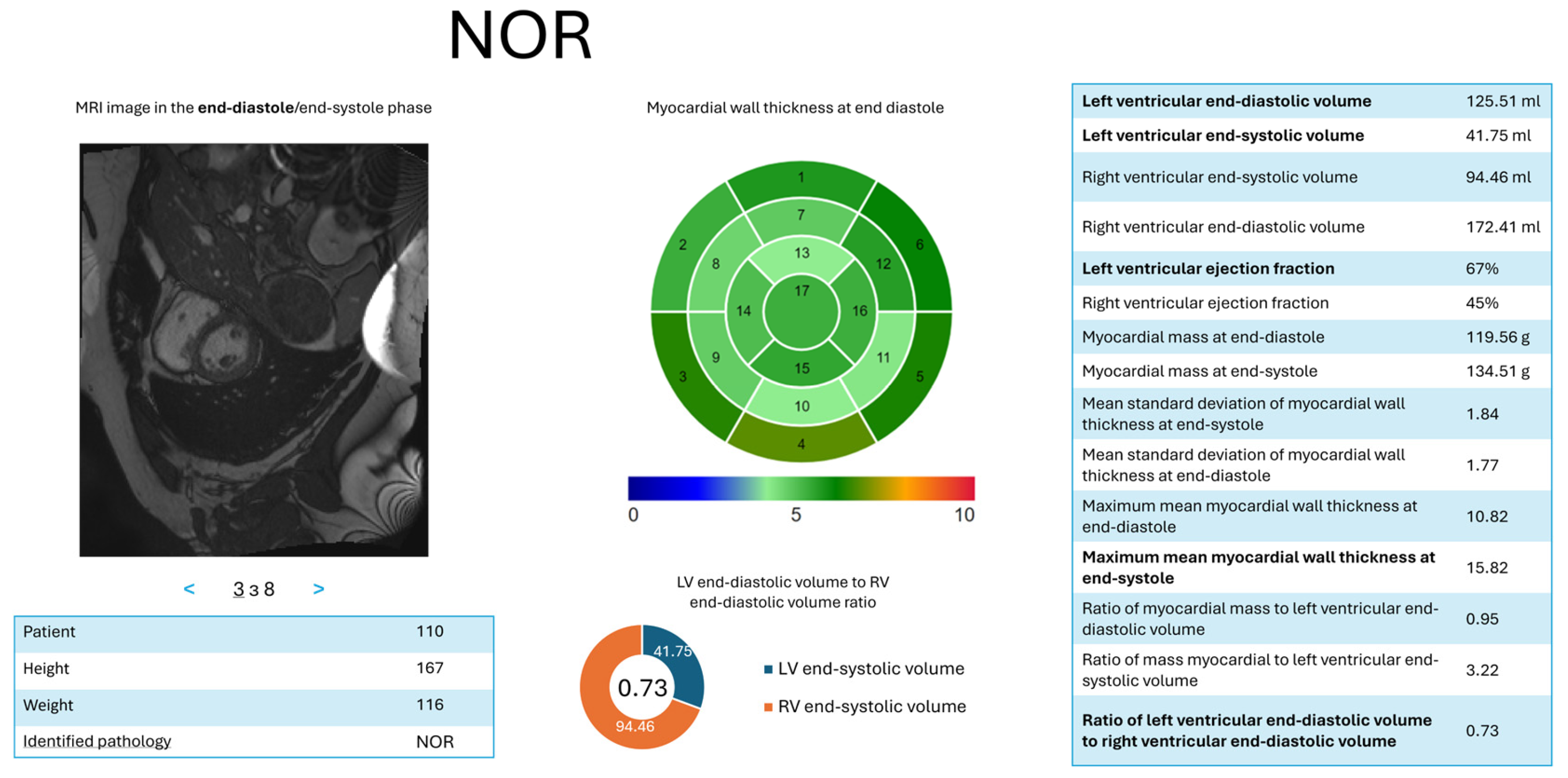
Normal State (NOR). In Figure A4 in Appendix A, the patient’s LV exhibits near-normal ES volume (feature ) of 41.75 ml, ED volume (feature ) of 125.51 ml, and an ejection fraction (feature ) of 67%, all consistent with healthy cardiac function. The RV volumes and ejection fraction lie within acceptable limits, and myocardial thickness remains stable. Together, these findings confirm the absence of significant pathology.
Overall, each pathology displays a unique profile of volumetric and functional changes: DCM is dominated by LV dilation; HCM shows asymmetric hypertrophy; MINF frequently reveals reduced EF with tissue irregularities; ARV reflects severe RV enlargement; and NOR remains within healthy ranges. The proposed interpretation approach clarifies each classification outcome in clinical terms by highlighting the most relevant quantitative features and visual cues.
4.4. Limitations of the Proposed Methods
Although the proposed methods for myocardium segmentation in the LV and RV show promise, certain limitations require attention.
Firstly, the model’s performance can deteriorate significantly when processing low-quality MRI scans. This issue is especially noticeable when parts of the myocardium or ventricles are not fully visible, resulting in incorrect segmentations or complete omission of these regions. The model heavily relies on detecting differences between the target structures and surrounding tissues; thus, poor image quality seriously affects accuracy.
Another challenge arises when image brightness levels are too low or too high (Figure 20). In such cases, the model may have difficulty correctly defining the boundaries of cardiac structures, resulting in poorly delineated segmentations. This occurs because areas with insufficient or excessive brightness lose crucial detail, negatively affecting model training quality.
Furthermore, the training data used to develop the models lacked sufficient examples of certain pathological conditions, such as cardiomyopathy or noncompaction myocardium. This shortage of samples may reduce the model’s ability to generalize to more complex conditions, thus affecting its reliability in clinical settings.
Finally, in some images, specific segments fail to visualize or only partially appear. In many cases, this arises from unfortunate slice timing—for example, capturing the moment the mitral or tricuspid valve is opening. The model may produce inaccurate results if the segments are not clearly visible in the image. Figure 21 shows that the lower part of the myocardium is poorly visualized but is still marked in the mask. Such masks may automatically train the network to fill these areas for similar cases.
Hence, although the approach is reliable under ideal conditions, its effectiveness strongly depends on the quality of the input data. Extra caution is needed when working with low-quality images or rare pathologies, as these factors can reduce accuracy and make the model less dependable in critical diagnostic situations.
4.5. Discussion of the Results
Each stage of the proposed multi-stage MRI segmentation method was examined during the experiments—from processing the original images to a comprehensive approach that includes localization, decomposition, and postprocessing. Each step contributed to improved accuracy in segmenting cardiac structures, as confirmed by the Dice coefficient for ED and ES phases. In the initial stage, segmenting the original images without localization or decomposition resulted in limited accuracy due to the influence of background noise and structural overlap. The final stage, which encompassed localization, mask decomposition, and postprocessing, achieved the best results. The proposed method effectively removed residual artifacts, smoothed contours, and improved the consistency of masks relative to expert annotations. This outcome confirmed the effectiveness of the proposed method, which combines all key processing steps: localization, decomposition, and postprocessing.
The proposed segmentation method achieved high accuracy: the Dice coefficient for the LV reached 0.974 in the ED phase and 0.940 in the ES phase. For the RV, the corresponding values were 0.947 and 0.915. The LV myocardium was segmented at 0.896 accuracy in diastole and 0.920 in systole, making it a promising tool for clinical applications and further research. According to a practicing cardiologist, 97.73% of the masks are satisfactory and of sufficient quality for medical analysis. The remaining 2.27% have poorer results mainly due to the low quality of the input images—specifically, suboptimal cardiac visualization owing to low resolution or image artifacts such as blurring (caused by patient movement during the MRI examination), low brightness, or low contrast (stemming from the MRI equipment’s limitations or technical challenges in a particular patient’s examination).
The introduced cascade classification method for detecting cardiac pathologies in MRI scans also shows high accuracy. Using separate classifiers at each stage provided considerable precision and consistency, even for challenging cases. The model achieved an overall accuracy of 97%, surpassing most current methods presented in the literature. Further experiments using multiclass classifiers ResNet-50 and ResNet-18 highlighted their limitations: ResNet-50 reached 84% accuracy, indicating difficulties in distinguishing similar classes such as MINF and DCM, while ResNet-18 (with fewer parameters) scored even lower at 72%, underscoring its insufficient capacity for complex classification tasks. These findings emphasize the advantages of the proposed step-by-step approach, which effectively accommodates each class’s specific characteristics. Comparisons with contemporary methods further confirmed the competitive nature of the proposed technique. Its high accuracy and adaptability make it promising for clinical integration, where robust classification performance and the ability to handle complex medical data are crucial.
The designed method for interpreting results allows a clear, structured presentation of medical data analysis outcomes. Adaptive visualization techniques—such as the 17-segment model, circular charts, and numerical values—offer clinicians an intuitive grasp of the results. This presentation style simplifies the diagnostic process and facilitates the incorporation of the findings into clinical practice.
5. Conclusions
This study introduces a set of novel methods for processing and evaluating cardiac MRI scans with higher precision and clarity. First, region extraction was refined by combining image resizing, specialized feature extraction layers, and further enhancements like postprocessing to smooth boundaries and minimizing artifacts. These steps boosted segmentation accuracy for the LV, RV, and myocardium. Second, classification was performed by separating classes into multiple phases, allowing the model to specialize in distinguishing particular sets of heart conditions. This phased approach raised a high overall accuracy, even for challenging pathologies such as those characterized by overlapping visual cues. Third, a metric-based interpretation scheme was developed, converting raw outputs into understandable clinical parameters, including ventricular volumes, wall thickness, and ejection fractions. By highlighting these features, the system provides transparency for physicians who must verify how diagnoses align with known cardiac metrics.
The numerical improvements are persuasive: a Dice coefficient of 0.974 for the LV, 0.947 for the RV, and 0.896–0.920 for the myocardium underscore the effectiveness of the proposed region delineation. Classification benchmarks also showed consistently high performance (97%), far outpacing established reference architectures. However, several limitations remain. Specifically, low-quality MRIs, i.e., poor resolution, motion artifacts, and brightness imbalances, can undermine segmentation and classification results. Moreover, limited training examples for certain rare pathologies hamper the model’s generalizability, suggesting additional data-gathering efforts are needed.
Future prospects include validating these methods across more diverse imaging protocols and rare cardiac conditions to ensure consistent performance. Furthermore, investigations into semi-supervised or self-supervised learning techniques may improve accuracy and reduce reliance on extensive annotations.
Author Contributions
Conceptualization, O.B. and I.K.; methodology, V.S. and O.B.; software, V.S.; validation, V.S., O.B. and L.K.; formal analysis, V.S., O.B. and P.R.; investigation, V.S.; resources, P.R. and L.K.; data curation, P.R. and L.K.; writing–original draft preparation, V.S. and O.B.; writing–review and editing, P.R., L.K. and I.K.; visualization, V.S. and P.R.; supervision, I.K. and O.B.; project administration, I.K. All authors have read and agreed to the published version of the manuscript.
Funding
This research received no external funding.
Data Availability Statement
Publicly available datasets were analyzed in this study. This data can be found here: https://github.com/vitalii-slobodzian/cardiac-mri-analysis/tree/develop (accessed on 15 January 2024).
Conflicts of Interest
The authors declare no conflicts of interest.
Abbreviations
The following abbreviations are used in this manuscript:
| ACDC | Automated Cardiac Diagnosis Challenge |
| AI | Artificial Intelligence |
| ARV | Abnormal Right Ventricle |
| AUC | Area Under the Curve, a performance measurement for classification models |
| CNN | Convolutional Neural Network |
| CT | Computed Tomography |
| DCM | Dilated Cardiomyopathy |
| DenseNet | Densely Connected Convolutional Networks |
| Dice | Dice Coefficient |
| DL | Deep Learning |
| D-TCAV | Deep Taylor Concept Activation Vector |
| ED | End-Diastole |
| ES | End-Systole |
| F1-score | F1 Score, the harmonic mean of precision and recall |
| HCM | Hypertrophic Cardiomyopathy |
| LV | Left Ventricle |
| MLP | Multilayer Perceptron |
| MRI | Magnetic Resonance Imaging |
| NOR | Normal State |
| ResNet | Residual Neural Network |
| RGB | Red, Green, Blue (color channels) |
| ROC | Receiver Operating Characteristic |
| ROI | Region of Interest |
| RV | Right Ventricle |
| SVM | Support Vector Machine |
Appendix A
Figure A1.
Visualization of HCM, illustrating thickened myocardial segments and high ejection fraction.
Figure A1.
Visualization of HCM, illustrating thickened myocardial segments and high ejection fraction.
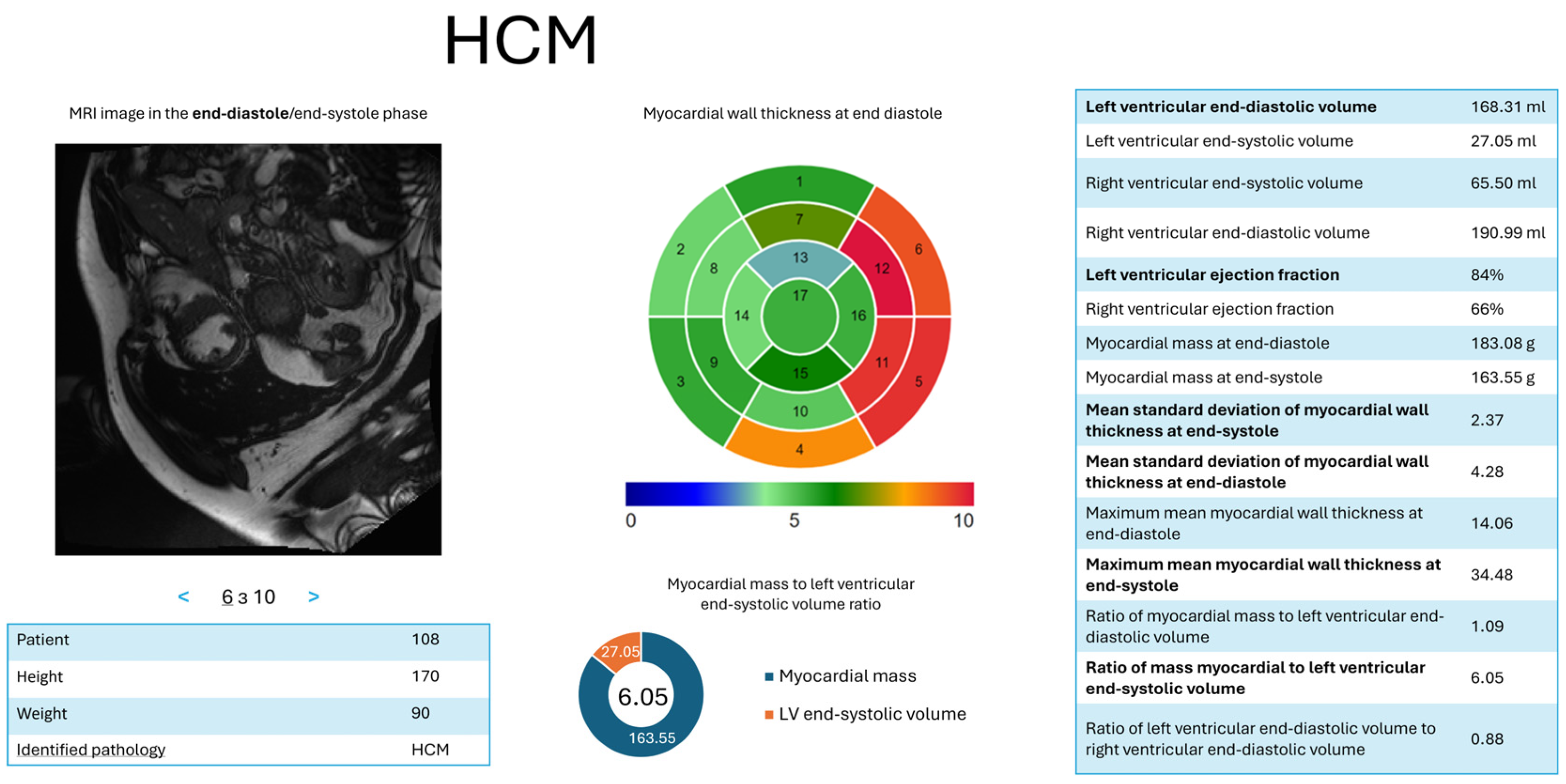
Figure A2.
Visualization of MINF, highlighting reduced ejection fraction and irregular myocardium thickness.
Figure A2.
Visualization of MINF, highlighting reduced ejection fraction and irregular myocardium thickness.
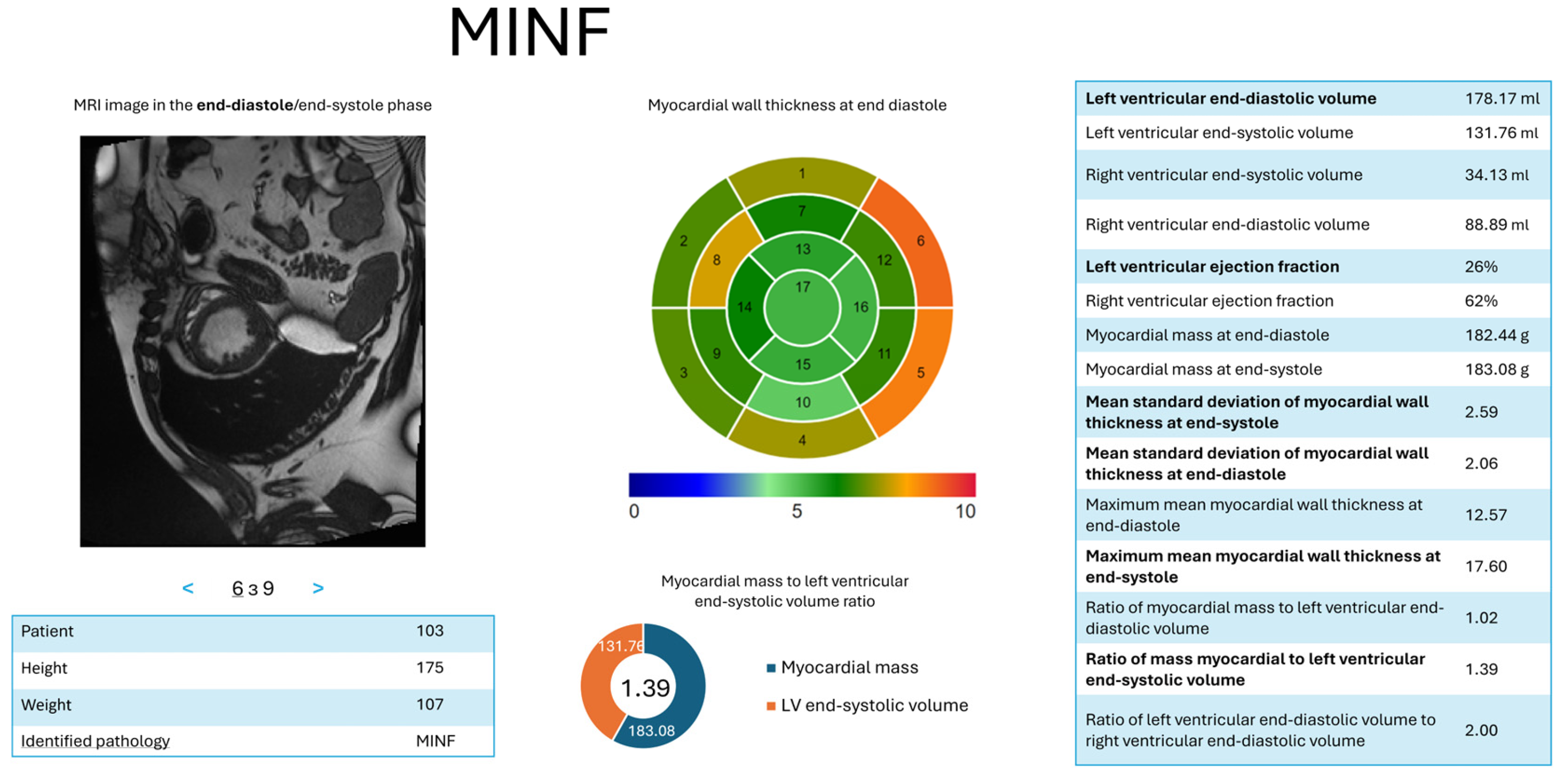
Figure A3.
Visualization of ARV, illustrating enlarged RV and weakened systolic performance.
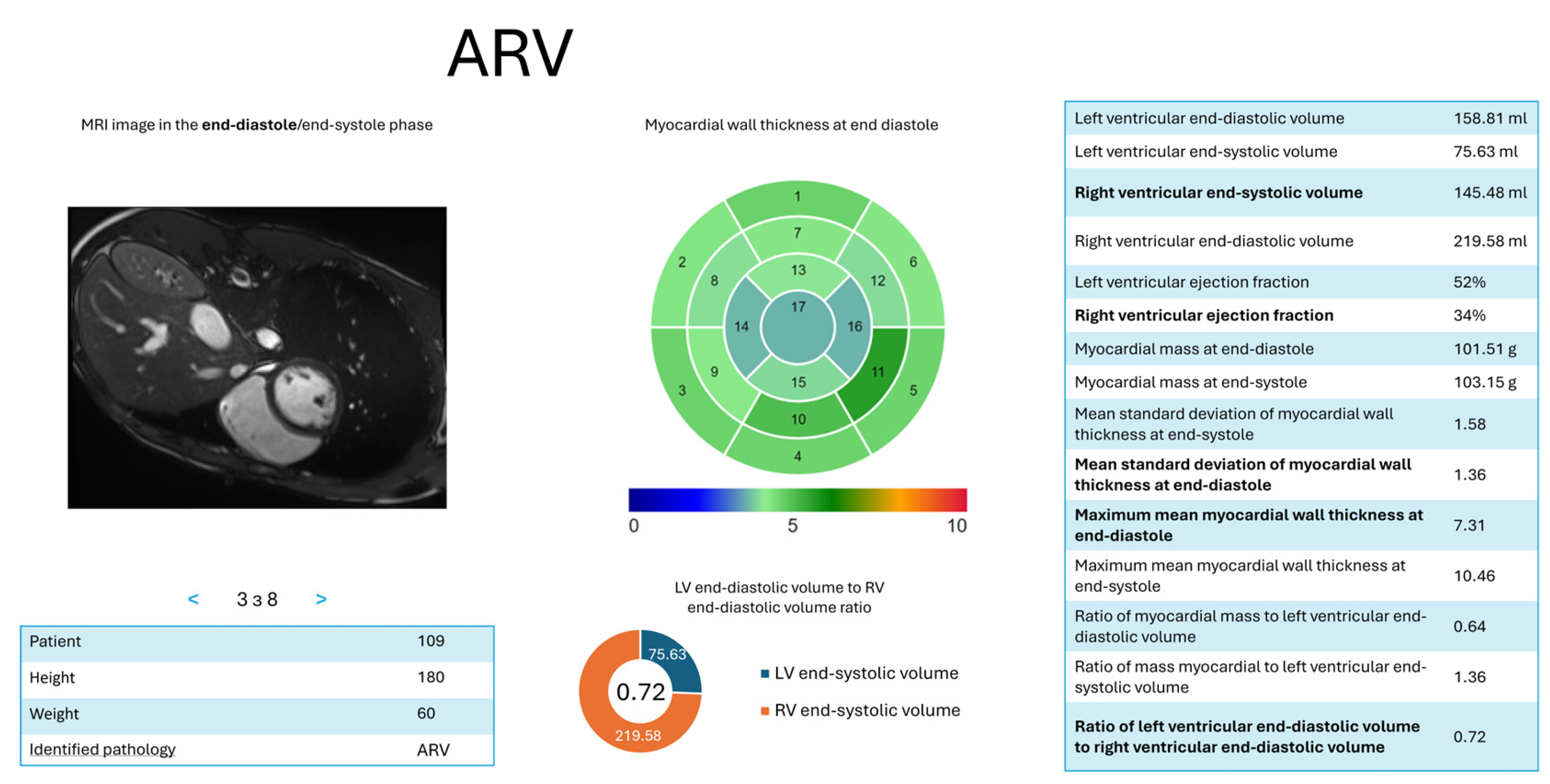
Figure A4.
Visualization of NOR, emphasizing balanced ventricular volumes and normal contractility.
References
- Morales, M. A.; Manning, W. J.; Nezafat, R. Present and future innovations in AI and cardiac MRI. Radiology 2024, 310, e231269. [Google Scholar] [CrossRef] [PubMed]
- Srinivasan, S.M.; Sharma, V. Applications of AI in cardiovascular disease detection—A review of the specific ways in which AI is being used to detect and diagnose cardiovascular diseases. In AI in Disease Detection; John Wiley & Sons, Ltd., 2025; Volume 6, pp. 123–146 ISBN 978-1-394-27869-5.
- Ball, J. R.; Balogh, E. Improving diagnosis in health care: Highlights of a report from the national academies of sciences, engineering, and medicine. Ann. Intern. Med. 2016, 164, 59–61. [Google Scholar] [CrossRef]
- Invisible numbers: The true extent of noncommunicable diseases and what to do about them; World Health Organization: Geneva, 2022; p. 42; Licence: CC BY-NC-SA 3.0 IGO.
- Counseller, Q.; Aboelkassem, Y. Recent technologies in cardiac imaging. Front. Med. Technol. 2023, 4, 984492. [Google Scholar] [CrossRef] [PubMed]
- Rose, N.E.; Gold, S.M. A comparison of accuracy between clinical examination and magnetic resonance imaging in the diagnosis of meniscal and anterior cruciate ligament tears. Arthroscopy: The Journal of Arthroscopic & Related Surgery 1996, 12, 398–405. [Google Scholar] [CrossRef]
- Kramer, C. M.; Barkhausen, J.; Bucciarelli-Ducci, C.; Flamm, S. D.; Kim, R. J.; Nagel, E. Standardized cardiovascular magnetic resonance imaging (CMR) protocols: 2020 update. J. Cardiovasc. Magn. Reson. 2020, 22. [Google Scholar] [CrossRef] [PubMed]
- Haskell, M. W.; Nielsen, J.; Noll, D. C. Off-resonance artifact correction for magnetic resonance imaging: A review. NMR Biomed. 2023, 36, e4867. [Google Scholar] [CrossRef] [PubMed]
- DeBenedectis, C. M.; Spalluto, L. B.; Americo, L.; Bishop, C.; Mian, A.; Sarkany, D.; Kagetsu, N. J.; Slanetz, P. J. Health care disparities in radiology—A review of the current literature. J. Am. Coll. Radiol. 2022, 19, 101–111. [Google Scholar] [CrossRef] [PubMed]
- Meidert, U.; Dönnges, G.; Bucher, T.; Wieber, F.; Gerber-Grote, A. Unconscious bias among health professionals: A scoping review. Int. J. Environ. Res. Public Health 2023, 20, 6569. [Google Scholar] [CrossRef]
- Radiuk, P.; Barmak, O.; Manziuk, E.; Krak, I. Explainable deep learning: A visual analytics approach with transition matrices. Mathematics 2024, 12, 1024. [Google Scholar] [CrossRef]
- Shick, A. A.; Webber, C. M.; Kiarashi, N.; Weinberg, J. P.; Deoras, A.; Petrick, N.; Saha, A.; Diamond, M. C. Transparency of artificial intelligence/machine learning-enabled medical devices. NPJ Digit. Med. 2024, 7, 12. [Google Scholar] [CrossRef]
- Radiuk, P.; Barmak, O.; Krak, I. An approach to early diagnosis of pneumonia on individual radiographs based on CNN information technology. Open Bioinform. J. 2021, 14, 93–107. [Google Scholar] [CrossRef]
- Zhao, Y.-q.; Gui, W.-h.; Chen, Z.-c.; Tang, J.-t.; Li, L.-y. Medical images edge detection based on mathematical morphology. In 2005 IEEE Engineering in Medicine and Biology 27th Annual Conference, Proceedings, Shanghai, China, January 17–18, 2006; IEEE: New York, NY, USA, 2005; pp. 6492–6495. [Google Scholar] [CrossRef]
- Xu, A.; Wang, L.; Feng, S.; Qu, Y. Threshold-based level set method of image segmentation. In 2010 3rd International Conference on Intelligent Networks and Intelligent Systems (ICINIS), Shenyang, China, November 1–3, 2010; IEEE: New York, NY, USA, 2010; pp. 703–706. [Google Scholar] [CrossRef]
- Cigla, C.; Alatan, A. A. Region-based image segmentation via graph cuts. In 2008 IEEE 16th Signal Processing, Communication and Applications Conference (SIU), Aydin, April 20–22, 2008; IEEE: New York, NY, USA, 2008; pp. 2272–2275. [Google Scholar] [CrossRef]
- Liu, X.; Song, L.; Liu, S.; Zhang, Y. A review of deep-learning-based medical image segmentation methods. Sustainability 2021, 13, 1224. [Google Scholar] [CrossRef]
- Berezsky, O.; Liashchynskyi, P.; Pitsun, O.; Izonin, I. Synthesis of convolutional neural network architectures for biomedical image classification. Biomed. Signal Process. Control 2024, 95, 106325. [Google Scholar] [CrossRef]
- Ronneberger, O.; Fischer, P.; Brox, T. U-Net: Convolutional networks for biomedical image segmentation. In Lecture Notes in Computer Science; Springer International Publishing: Cham, 2015; pp. 234–241. [Google Scholar] [CrossRef]
- Badrinarayanan, V.; Kendall, A.; Cipolla, R. SegNet: A deep convolutional encoder-decoder architecture for image segmentation. IEEE Trans. Pattern Anal. Mach. Intell. 2017, 39, 2481–2495. [Google Scholar] [CrossRef] [PubMed]
- Ankenbrand, M. J.; Lohr, D.; Schlötelburg, W.; Reiter, T.; Wech, T.; Schreiber, L. M. Deep learning-based cardiac cine segmentation: Transfer learning application to 7T ultrahigh-field MRI. Magn. Reson. Med. 2021, 86, 2179–2191. [Google Scholar] [CrossRef]
- Radiuk, P.; Kovalchuk, O.; Slobodzian, V.; Manziuk, E.; Krak, I. Human-in-the-loop approach based on MRI and ECG for healthcare diagnosis. In Proceedings of the 5th International Conference on Informatics & Data-Driven Medicine (IDDM-2022), Lyon, France, 18–20 November 2022; Shakhovska, N., Chretien, S., Izonin, I., Campos, J., Eds.; CEUR-WS: Aachen, Germany, 2022; Volume 3302, pp. 9–20. [Google Scholar]
- Singh, A.; Singh, K. K.; Izonin, I. Responsible and explainable artificial intelligence in healthcare: Conclusion and future directions. In Responsible and Explainable Artificial Intelligence in Healthcare; Academic Press: Cambridge, MA, USA, 2025; с 285–297. [Google Scholar] [CrossRef]
- Wehbe, R. M.; Katsaggleos, A. K.; Hammond, K. J.; Hong, H.; Ahmad, F. S.; Ouyang, D.; Shah, S. J.; McCarthy, P. M.; Thomas, J. D. Deep learning for cardiovascular imaging. JAMA Cardiol. 2023, 8, 1089–1098. [Google Scholar] [CrossRef] [PubMed]
- Pandey, S.; Chen, K.-F.; Dam, E. B. Comprehensive multimodal segmentation in medical imaging: Combining YOLOv8 with SAM and HQ-SAM models. In 2023 IEEE/CVF International Conference on Computer Vision Workshops (ICCVW), Paris, France, October 2–6, 2023; IEEE: New York, NY, USA, 2023; pp. 2592–2598. [Google Scholar] [CrossRef]
- Azam, M. A.; Khan, K. B.; Salahuddin, S.; Rehman, E.; Khan, S. A.; Khan, M. A.; Kadry, S.; Gandomi, A. H. A review on multimodal medical image fusion: Compendious analysis of medical modalities, multimodal databases, fusion techniques and quality metrics. Comput. Biol. Med. 2022, 144, 105253. [Google Scholar] [CrossRef]
- Hu, H.; Pan, N.; Frangi, A. F. Fully Automatic initialization and segmentation of Left and Right ventricles for Large-Scale cardiac MRI using a deeply supervised network and 3D-ASM. Comput. Methods Programs Biomed. 2023, 240, 107679. [Google Scholar] [CrossRef]
- da Silva, I. F. S. d.; Silva, A. C.; Paiva, A. C. d.; Gattass, M.; Cunha, A. M. A multi-stage automatic method based on a combination of fully convolutional networks for cardiac segmentation in short-axis MRI. Appl. Sci. 2024, 14, 7352. [Google Scholar] [CrossRef]
- Tian, Y.; Krishnan, D.; Isola, P. Contrastive multiview coding. In Computer Vision—ECCV 2020; Springer International Publishing: Cham, 2020; pp. 776–794. [Google Scholar] [CrossRef]
- Chen, T.; Kornblith, S.; Norouzi, M.; Hinton, G. E. A simple framework for contrastive learning of visual representations. In Proceedings of the 37th International Conference on Machine Learning, Virtual Event, July 13–18 2020; pp. 1597–1607. [Google Scholar]
- Liu, C.; Amodio, M.; Shen, L. L.; Gao, F.; Avesta, A.; Aneja, S.; Wang, J. C.; Del Priore, L. V.; Krishnaswamy, S. CUTS: A deep learning and topological framework for multigranular unsupervised medical image segmentation. In Lecture Notes in Computer Science; Springer Nature Switzerland: Cham, 2024; pp. 155–165. [Google Scholar] [CrossRef]
- Felfeliyan, B.; Forkert, N. D.; Hareendranathan, A.; Cornel, D.; Zhou, Y.; Kuntze, G.; Jaremko, J. L.; Ronsky, J. L. Self-supervised-RCNN for medical image segmentation with limited data annotation. Comput. Med. Imaging Graph. 2023, 109, 102297. [Google Scholar] [CrossRef] [PubMed]
- Zheng, Q.; Delingette, H.; Ayache, N. Explainable cardiac pathology classification on cine MRI with motion characterization by semi-supervised learning of apparent flow. Med. Image Anal. 2019, 56, 80–95. [Google Scholar] [CrossRef] [PubMed]
- Ammar, A.; Bouattane, O.; Youssfi, M. Automatic cardiac cine MRI segmentation and heart disease classification. Comput. Med. Imaging Graphics 2021, 88, 101864. [Google Scholar] [CrossRef] [PubMed]
- Bourfiss, M.; Sander, J.; de Vos, B. D.; te Riele, A. S. J. M.; Asselbergs, F. W.; Išgum, I.; Velthuis, B. K. Towards automatic classification of cardiovascular magnetic resonance Task Force Criteria for diagnosis of arrhythmogenic right ventricular cardiomyopathy. Clin. Res. Cardiol. 2023, 112, 363–378. [Google Scholar] [CrossRef] [PubMed]
- Mofrad, F. B.; Valizadeh, G. DenseNet-based transfer learning for LV shape classification: Introducing a novel information fusion and data augmentation using statistical shape/color modeling. Expert Syst. With Appl. 2022, 213, 119261. [Google Scholar] [CrossRef]
- He, K.; Zhang, X.; Ren, S.; Sun, J. Deep residual learning for image recognition. In 2016 IEEE Conference on Computer Vision and Pattern Recognition (CVPR), Las Vegas, NV, USA, June 27–30, 2016; IEEE: New York, NY, USA, 2016; pp. 770–778. [Google Scholar] [CrossRef]
- Huang, G.; Liu, Z.; Van Der Maaten, L.; Weinberger, K. Q. Densely connected convolutional networks. In 2017 IEEE Conference on Computer Vision and Pattern Recognition (CVPR), Honolulu, HI, USA, July 21–26, 2017; IEEE: New York, NY, USA, 2017; pp. 4700–4708. [Google Scholar] [CrossRef]
- Isensee, F.; Jaeger, P. F.; Full, P. M.; Wolf, I.; Engelhardt, S.; Maier-Hein, K. H. Automatic cardiac disease assessment on cine-MRI via time-series segmentation and domain specific features. In Lecture Notes in Computer Science; Springer International Publishing: Cham, 2018; pp. 120–129. [Google Scholar] [CrossRef]
- Khened, M.; Kollerathu, V. A.; Krishnamurthi, G. Fully convolutional multi-scale residual DenseNets for cardiac segmentation and automated cardiac diagnosis using ensemble of classifiers. Med. Image Anal. 2019, 51, 21–45. [Google Scholar] [CrossRef]
- Watanabe, A.; Ketabi, S.; Namdar, K.; Khalvati, F. Improving disease classification performance and explainability of deep learning models in radiology with heatmap generators. Front. Radiol. 2022, 2, 991683. [Google Scholar] [CrossRef] [PubMed]
- Ali, M.; Olanisa, O. O.; Nzeako, T.; Shahrokhi, M.; Esfahani, E.; Fakher, N.; Tabari, M. A. K. Revolutionizing cardiac imaging: A scoping review of artificial intelligence in echocardiography, CTA, and cardiac MRI. J. Imaging 2024, 10, 193. [Google Scholar] [CrossRef]
- Szabo, L.; Raisi-Estabragh, Z.; Salih, A.; McCracken, C.; Ruiz Pujadas, E.; Gkontra, P.; Kiss, M.; Maurovich-Horvath, P.; Vago, H.; Merkely, B.; et al. Clinician’s guide to trustworthy and responsible artificial intelligence in cardiovascular imaging. Front. Cardiovasc. Med. 2022, 9, 1016032. [Google Scholar] [CrossRef]
- Janik, A.; Dodd, J.; Ifrim, G.; Sankaran, K.; Curran, K. M. Interpretability of a deep learning model in the application of cardiac MRI segmentation with an ACDC challenge dataset. In Image Processing, Online, February 15–19, 2021; Landman, B. A., Išgum, I., Eds.; SPIE: Bellingham, WA, USA, 2021; p. 1159636. [Google Scholar] [CrossRef]
- Wang, Y.; Jia, H.; Song, J. Accurate classification of non-ischemic cardiomyopathy. Curr. Cardiol. Rep. 2023, 25, 1299–1317. [Google Scholar] [CrossRef]
- McKenna, W. J.; Maron, B. J.; Thiene, G. Classification, epidemiology, and global burden of cardiomyopathies. Circ. Res. 2017, 121, 722–730. [Google Scholar] [CrossRef]
- Bernard, O.; Lalande, A.; Zotti, C.; Cervenansky, F. Deep learning techniques for automatic MRI cardiac multi-structures segmentation and diagnosis: Is the problem solved? IEEE Trans. Med. Imaging 2018, 37, 2514–2525. [Google Scholar] [CrossRef]
- Slobodzian, V.; Radiuk, P.; Zingailo, A.; Barmak, O.; Krak, I. Myocardium segmentation using two-step deep learning with smoothed masks by gaussian blur. In Proceedings of the 6th International Conference on Informatics & Data-Driven Medicine (IDDM-2023), Bratislava, Slovakia, 17–19 November 2023; hakhovska, N., Kovac, M., Izonin, I., Chretien, S., Eds.; CEUR-WS: Aachen, Germany, 2024; Volume 3609, pp. 77–91. [Google Scholar]
- Slobodzian, V.; Radiuk, P.; Barmak, O.; Krak, I. Multi-stage segmentation and cascade classification methods for improving cardiac MRI analysis. In Proceedings of the X International Scientific Conference “Information Technology and Implementation” (IT&I 2024), Kyiv, Ukraine, 20–21 November 2024; Anisimov, A., et al., Eds.; CEUR-WS: Aachen, Germany, 2025; Volume 3900, pp. 1–15. [Google Scholar]
- Izquierdo, C.; Casas, G.; Martin-Isla, C.; Campello, V. M.; Guala, A.; Gkontra, P.; Rodríguez-Palomares, J. F.; Lekadir, K. Radiomics-based classification of left ventricular non-compaction, hypertrophic cardiomyopathy, and dilated cardiomyopathy in cardiovascular magnetic resonance. Front. Cardiovasc. Med. 2021, 8, 764312. [Google Scholar] [CrossRef] [PubMed]
- Afshin, M.; Ben Ayed, I.; Punithakumar, K.; Law, M.; Islam, A.; Goela, A.; Peters, T.; Shuo, Li. Regional assessment of cardiac left ventricular myocardial function via MRI statistical features. IEEE Trans. Med. Imaging 2014, 33, 481–494. [Google Scholar] [CrossRef] [PubMed]
- Rainio, O.; Teuho, J.; Klén, R. Evaluation metrics and statistical tests for machine learning. Sci. Rep. 2024, 14, 6086. [Google Scholar] [CrossRef] [PubMed]
Figure 1.
The proposed task decomposition for cardiac MRI processing, illustrating the process flow from input MRI scans through three sequential processing stages—segmentation, classification, and interpretation of decisions—resulting in the output of predicted classes and interpretations.
Figure 1.
The proposed task decomposition for cardiac MRI processing, illustrating the process flow from input MRI scans through three sequential processing stages—segmentation, classification, and interpretation of decisions—resulting in the output of predicted classes and interpretations.
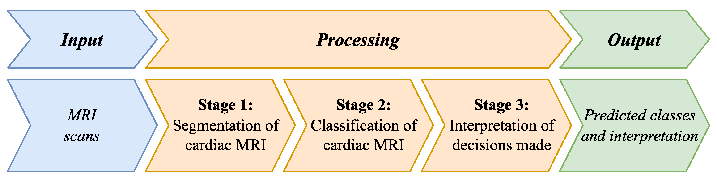
Figure 2.
The main steps for obtaining DL models for segmenting the LV, RV, and myocardium regions in an MRI scan.
Figure 2.
The main steps for obtaining DL models for segmenting the LV, RV, and myocardium regions in an MRI scan.
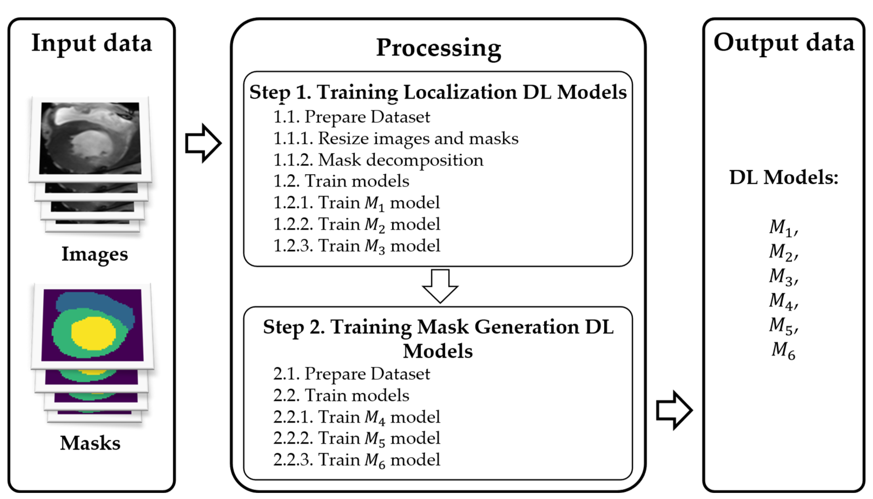
Figure 3.
The main steps for segmenting an MRI scan into regions of the LV, RV, and myocardium.
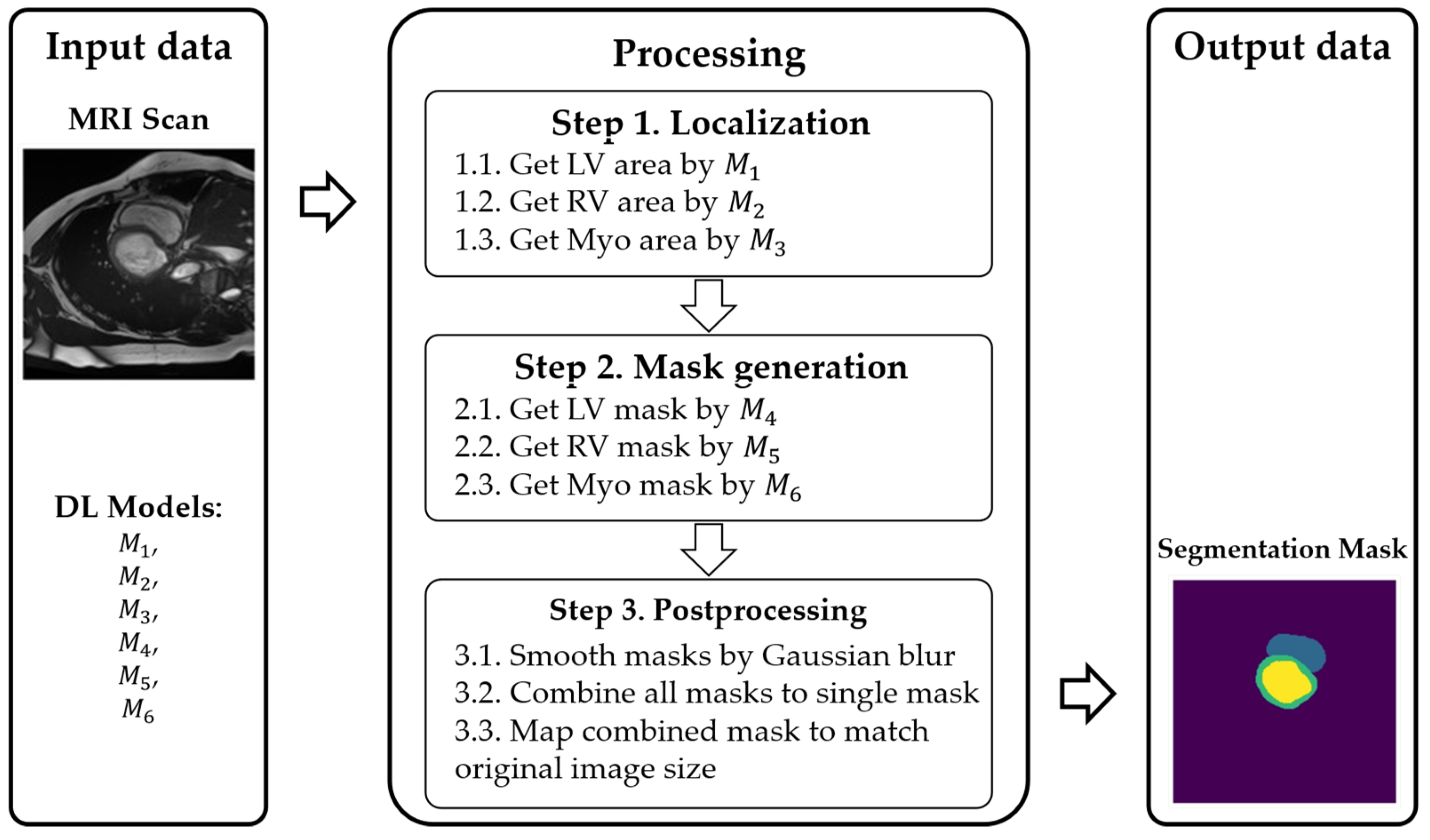
Figure 4.
Visualizations of the input data. The top row shows MRIs from the systolic phase, and the bottom row—is diastolic; each column is a short-axis slice with RV highlighted in red, LV—in blue, and myocardium—in green.
Figure 4.
Visualizations of the input data. The top row shows MRIs from the systolic phase, and the bottom row—is diastolic; each column is a short-axis slice with RV highlighted in red, LV—in blue, and myocardium—in green.
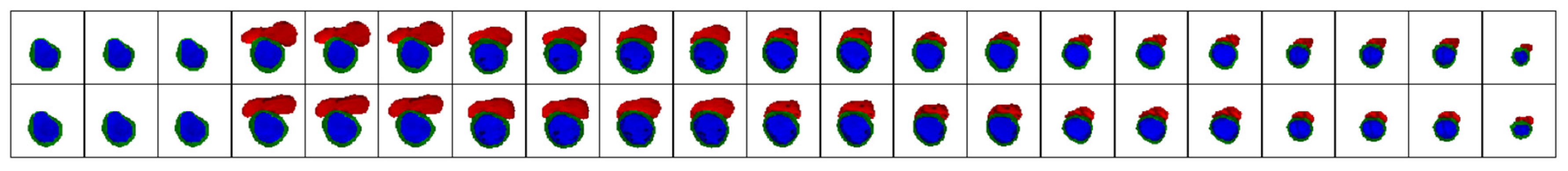
Figure 5.
Structure of the cascade classification into five classes: ARV, HCM, MINF, DCM, and NOR. Here, LV pathologies are HCM, MINF, and DCM.
Figure 5.
Structure of the cascade classification into five classes: ARV, HCM, MINF, DCM, and NOR. Here, LV pathologies are HCM, MINF, and DCM.
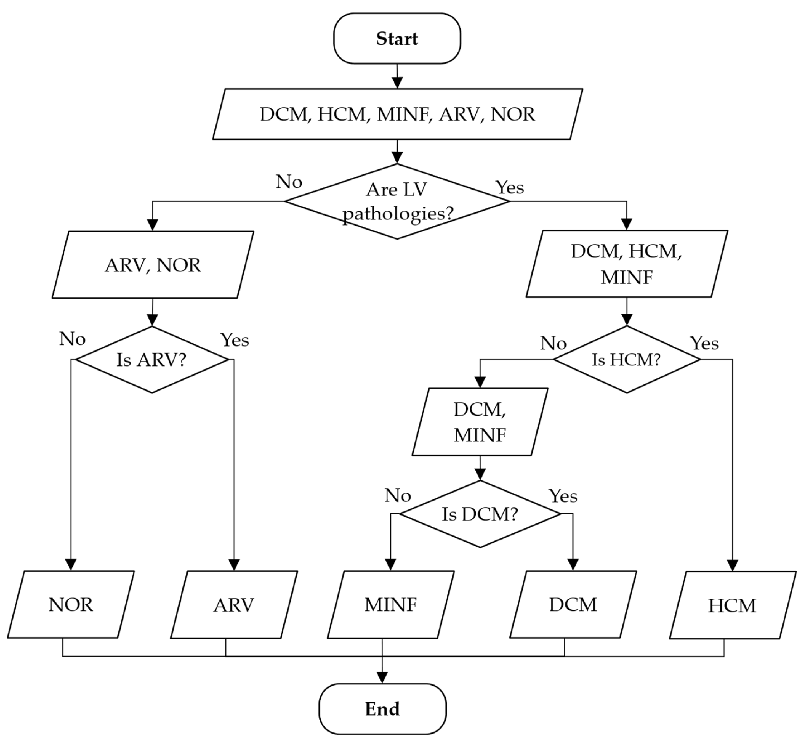
Figure 6.
Overall scheme of the training process for models , , , and .
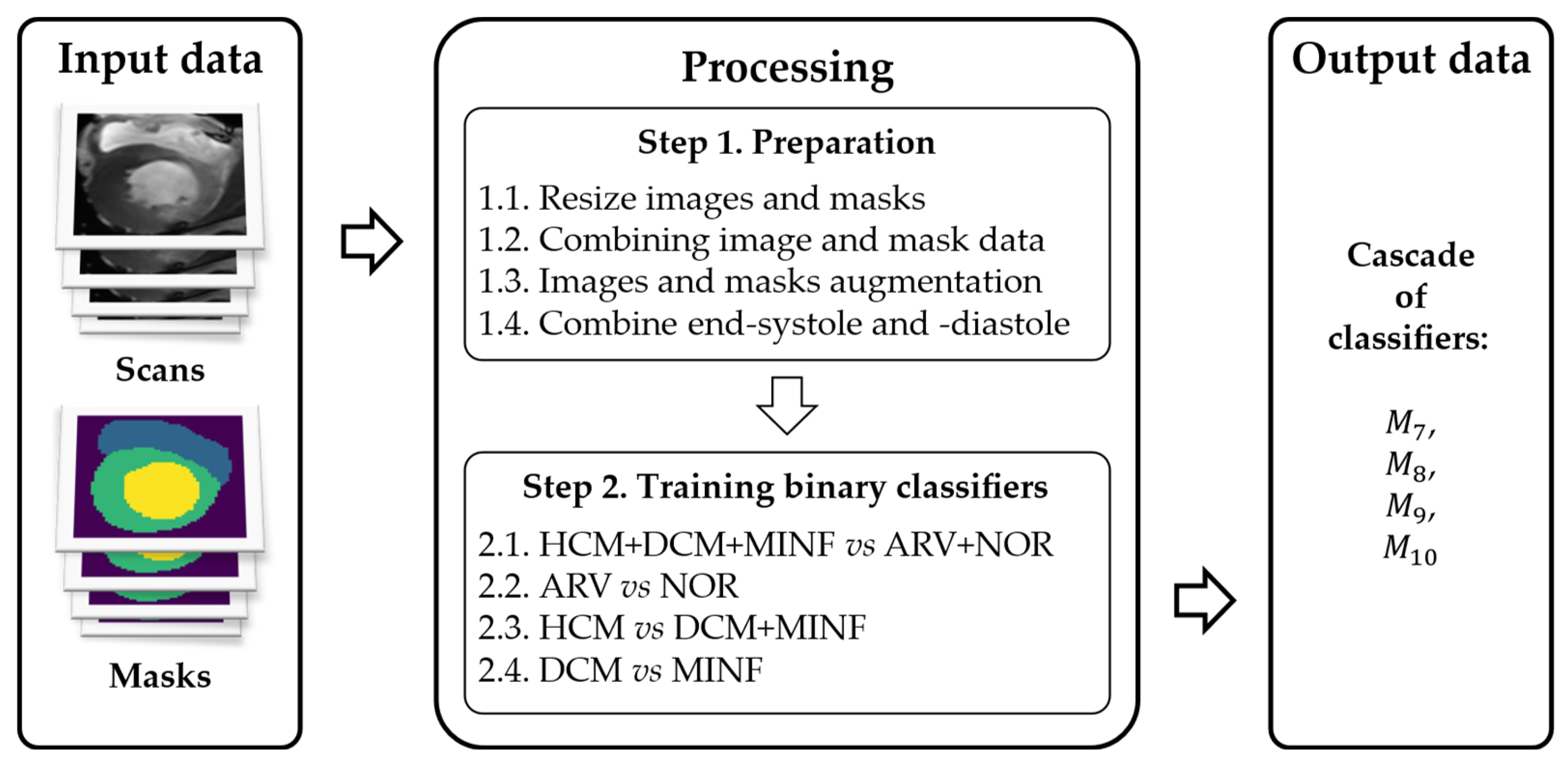
Figure 7.
Scheme of the pathology classification process using cardiac MRI of an arbitrary patient.
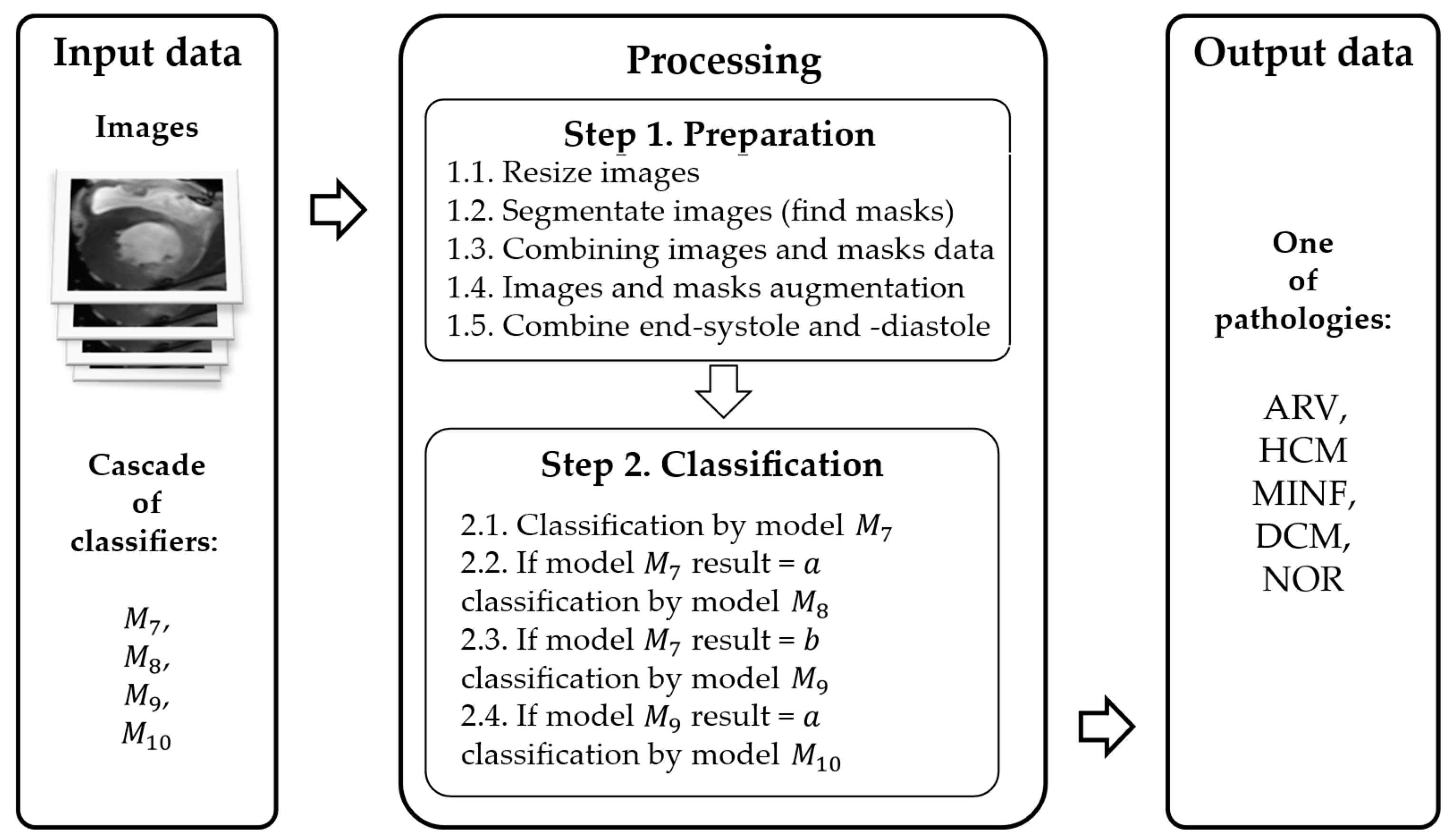
Figure 8.
The overall scheme of the proposed interpretation method.
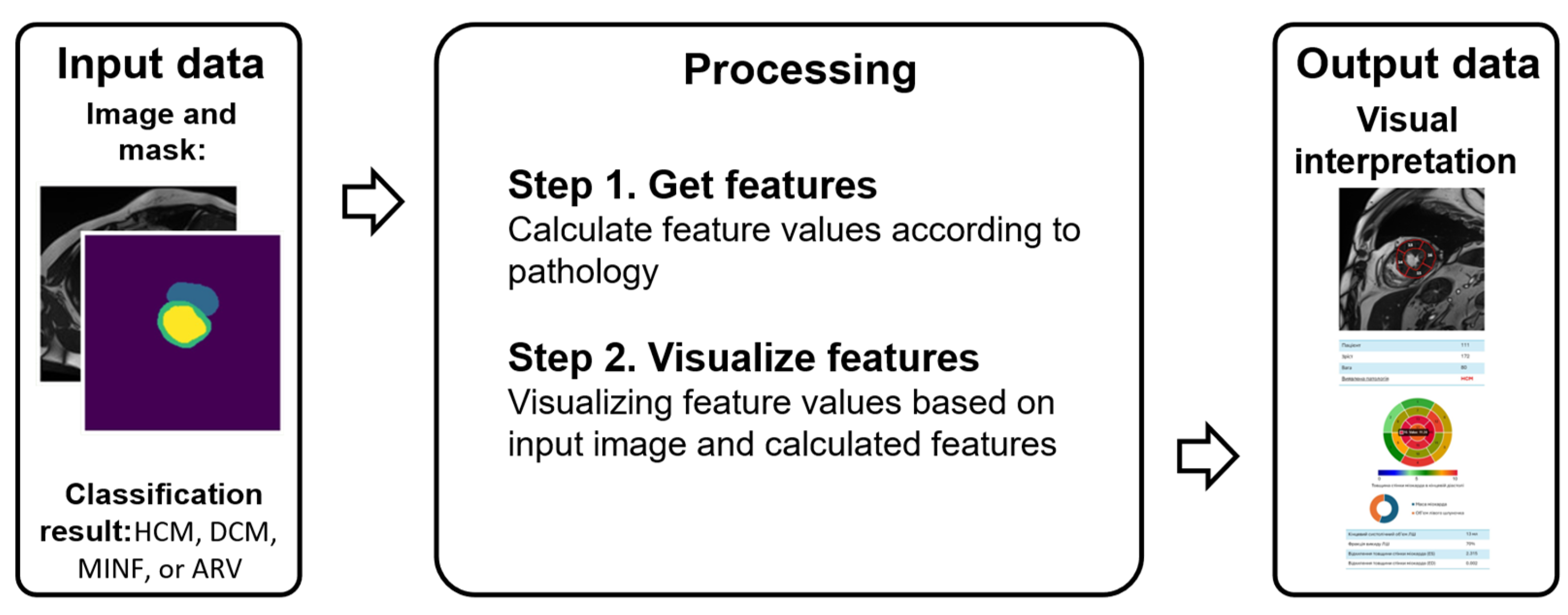
Figure 9.
Example from the dataset with a cardiac MRI scan (a) and its mask (b).
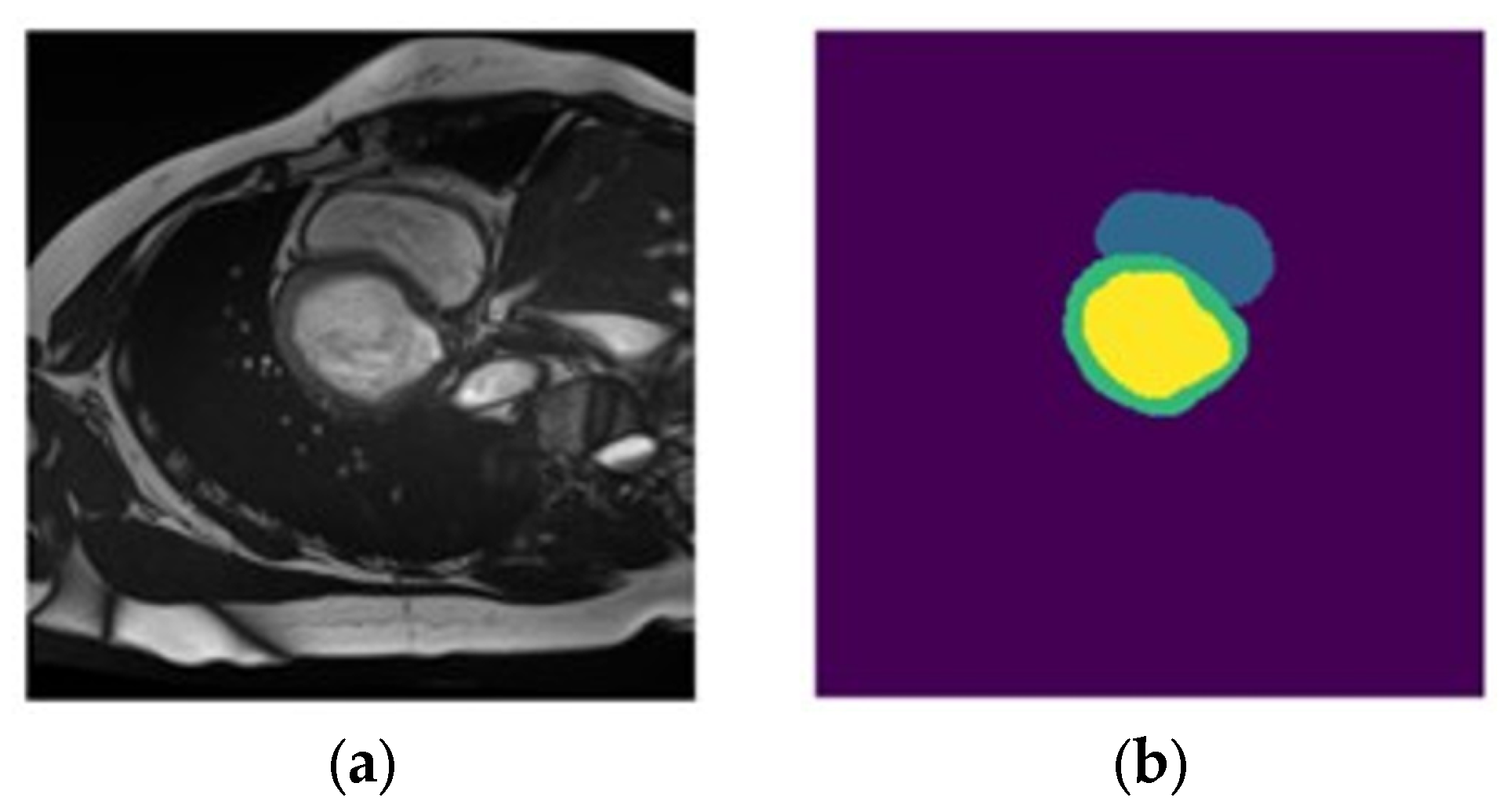
Figure 10.
Instance element of dataset : (a) MRI scan, (b) myocardium segment mask, (c) LV segment mask, and (d) RV segment mask.
Figure 10.
Instance element of dataset : (a) MRI scan, (b) myocardium segment mask, (c) LV segment mask, and (d) RV segment mask.
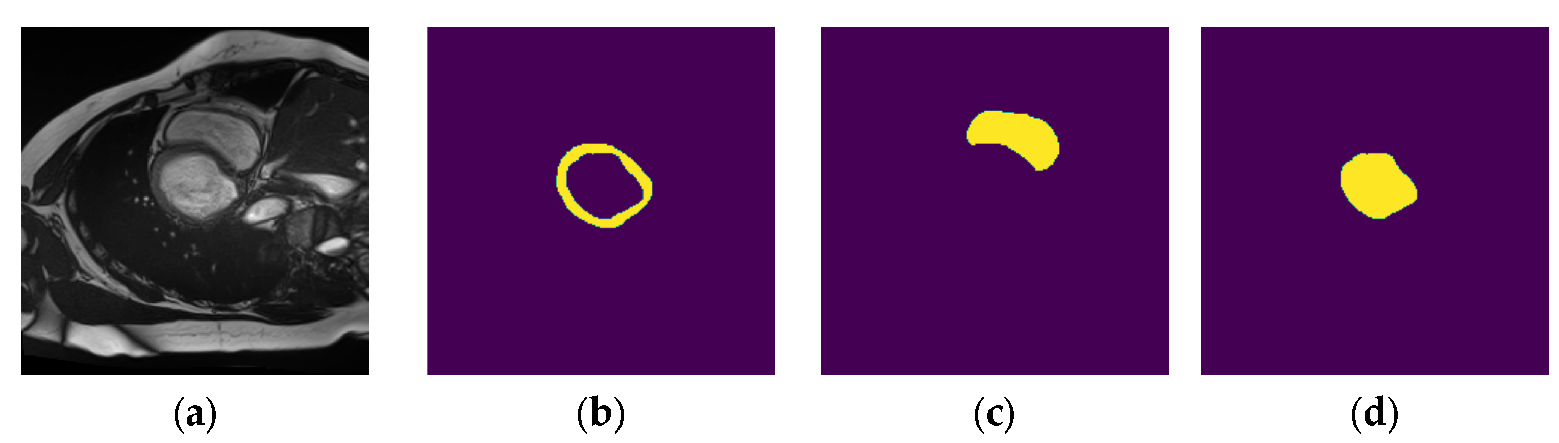
Figure 11.
Example elements of created datasets: —(a) MRI scan, (b) LV segment mask; —(c) MRI scan, (d) RV segment mask; —(e) MRI scan, (f) myocardium segment mask.
Figure 11.
Example elements of created datasets: —(a) MRI scan, (b) LV segment mask; —(c) MRI scan, (d) RV segment mask; —(e) MRI scan, (f) myocardium segment mask.
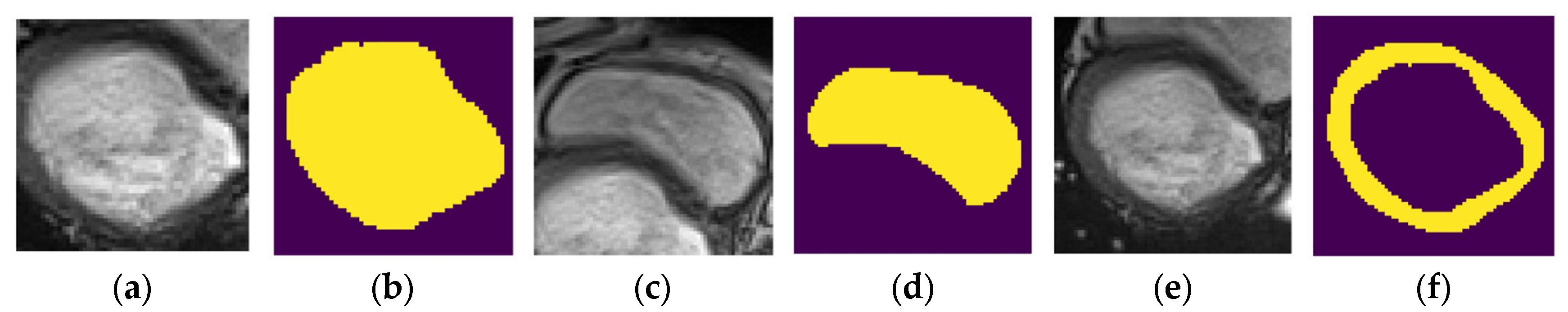
Figure 12.
Example element of dataset : (a) set of modified MRI scans and (b) pathology class label (MINF).
Figure 12.
Example element of dataset : (a) set of modified MRI scans and (b) pathology class label (MINF).
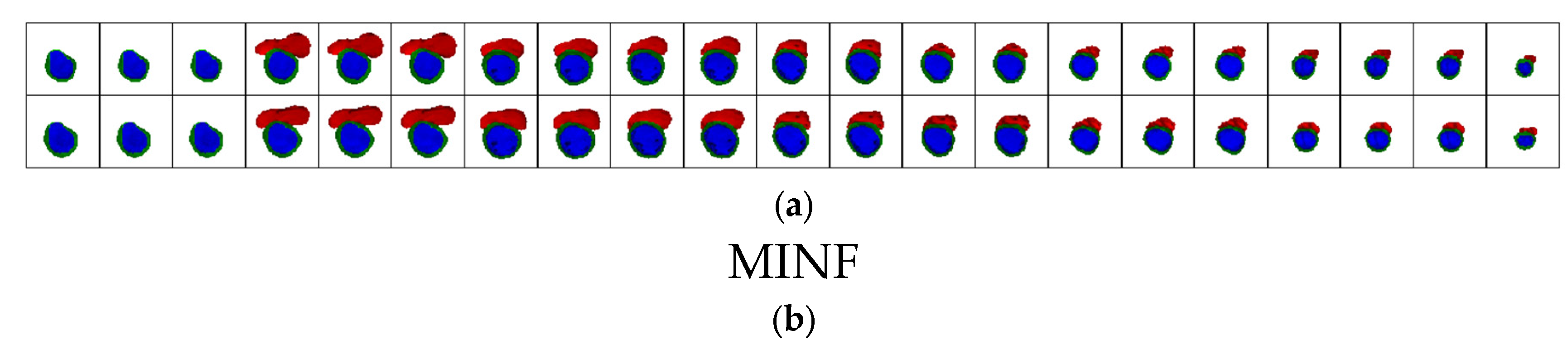
Figure 13.
Visual comparison of obtained Dice coefficient values for experiments 1–5 (ES—end-systole, ED—end-diastole).
Figure 13.
Visual comparison of obtained Dice coefficient values for experiments 1–5 (ES—end-systole, ED—end-diastole).
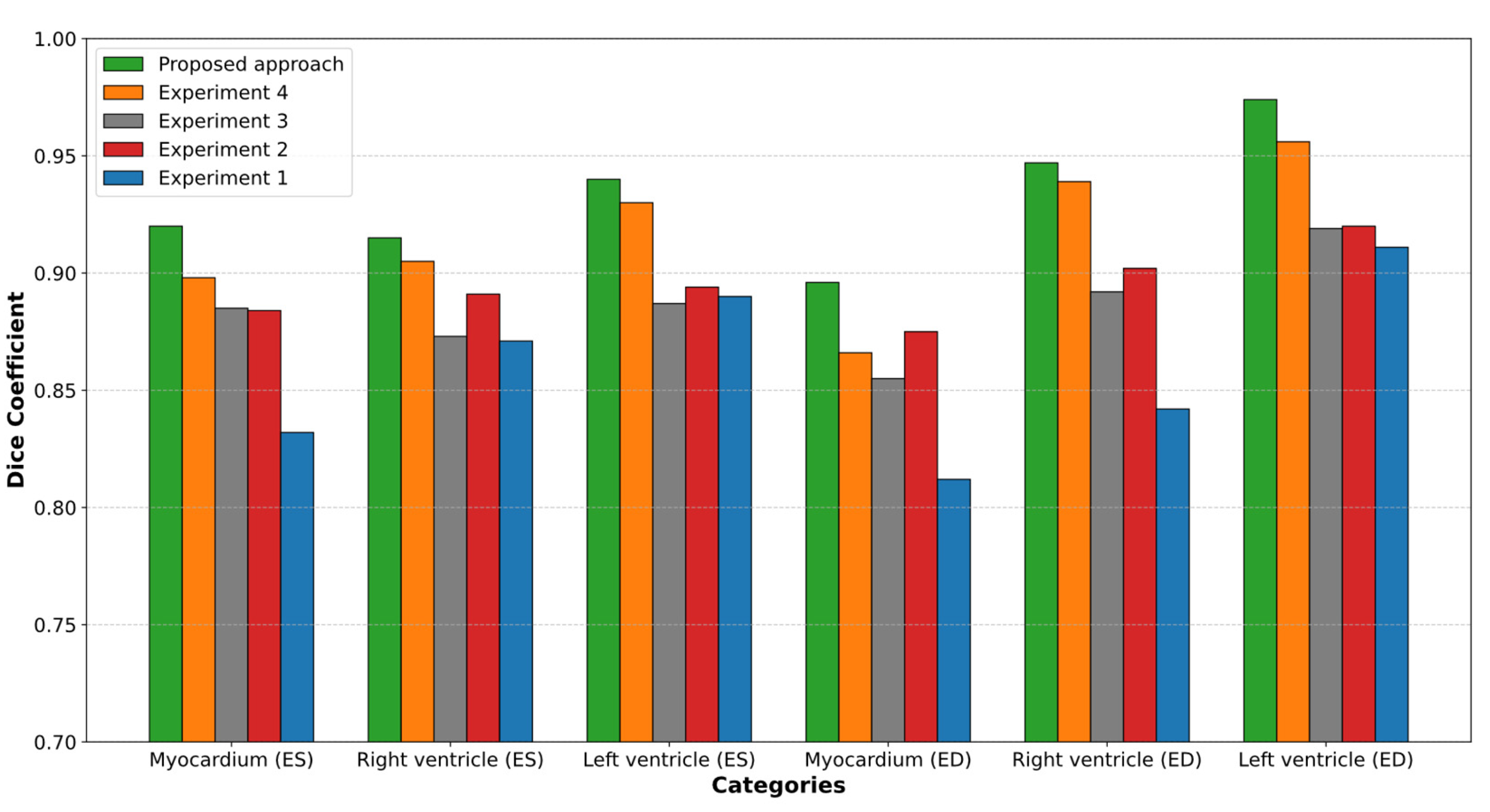
Figure 14.
Visual comparison of obtained Dice coefficient values with the state of the art (ES—end-systole, ED—end-diastole).
Figure 14.
Visual comparison of obtained Dice coefficient values with the state of the art (ES—end-systole, ED—end-diastole).
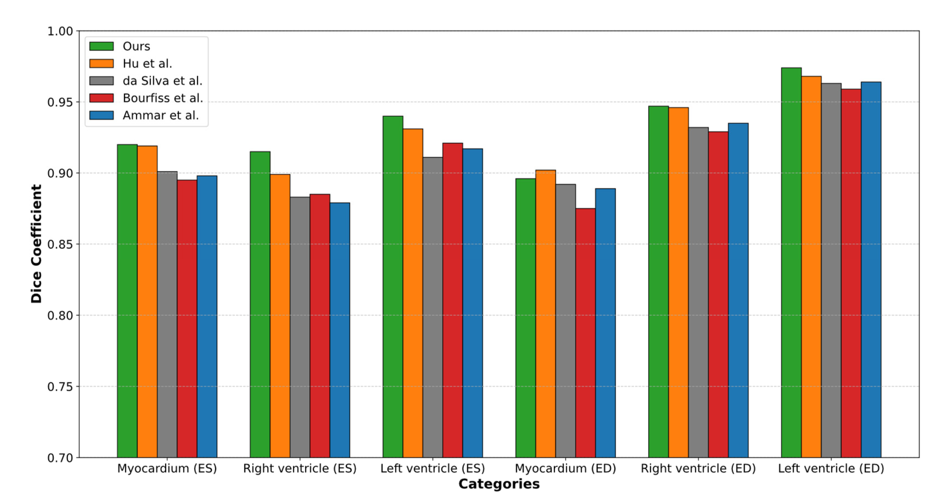
Figure 15.
Comparison of expert mask and mask generated by the proposed segmentation model: (a) expert mask, (b) mask obtained by the proposed method, and (c) difference between masks.
Figure 15.
Comparison of expert mask and mask generated by the proposed segmentation model: (a) expert mask, (b) mask obtained by the proposed method, and (c) difference between masks.
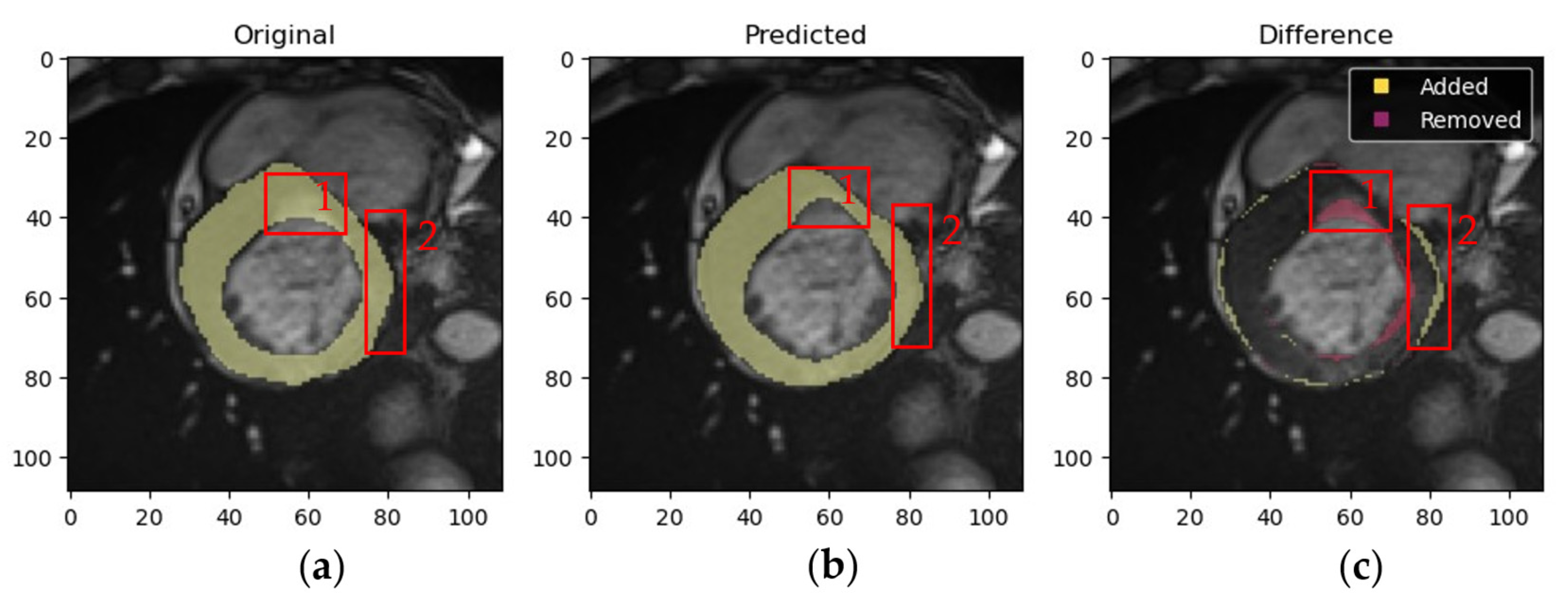
Figure 16.
Confusion matrices for multiclass classifiers using two architectures: (a) ResNet-50 and (b) ResNet-18, showcasing the classification performance across five classes, including NOR, MINF, DCM, HCM, and ARV.
Figure 16.
Confusion matrices for multiclass classifiers using two architectures: (a) ResNet-50 and (b) ResNet-18, showcasing the classification performance across five classes, including NOR, MINF, DCM, HCM, and ARV.
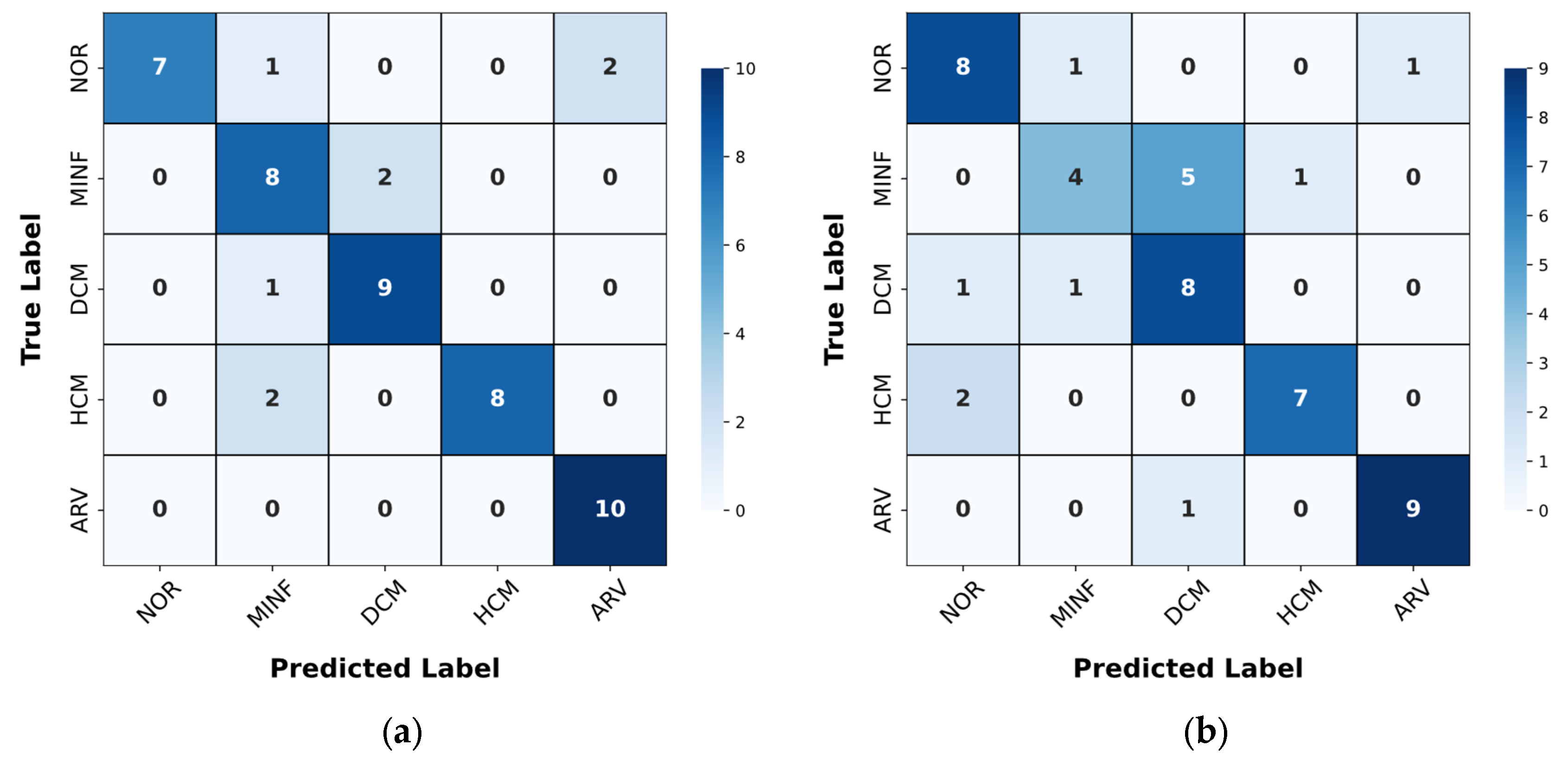
Figure 17.
Confusion matrices, illustrating classification performance across sequential steps: (a) Step 1—Classifier 1, (b) Step 2—Classifier 2, (c) Step 3—Classifier 3, and (d) Step 4—Classifier 4, highlighting the accuracy and misclassifications for labels A and B at each step of the process.
Figure 17.
Confusion matrices, illustrating classification performance across sequential steps: (a) Step 1—Classifier 1, (b) Step 2—Classifier 2, (c) Step 3—Classifier 3, and (d) Step 4—Classifier 4, highlighting the accuracy and misclassifications for labels A and B at each step of the process.
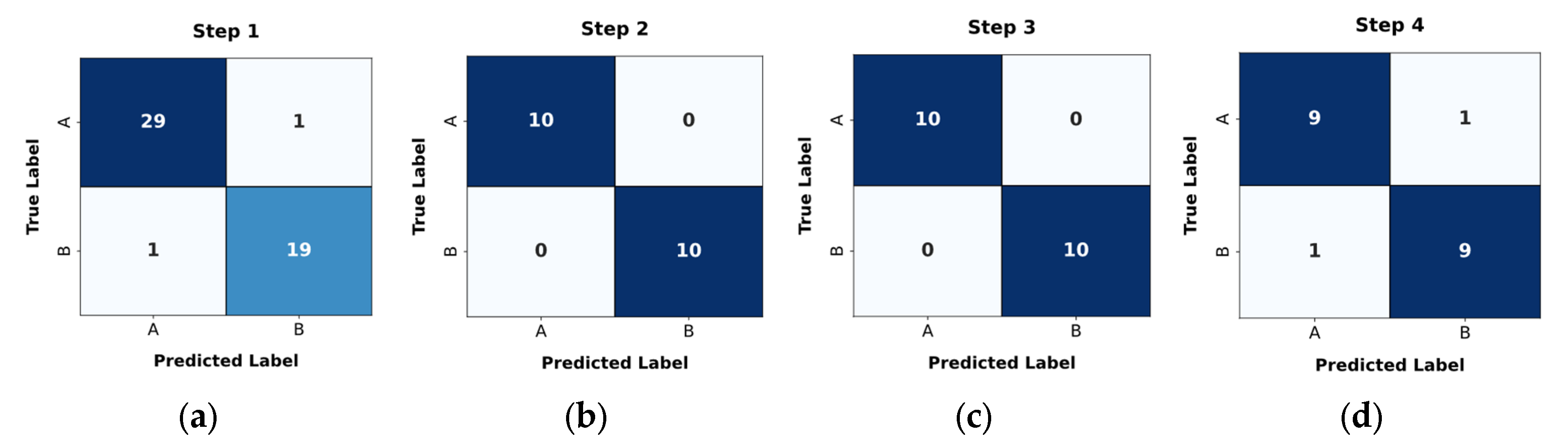
Figure 18.
ROC curves for classification steps, showing the true positive rate versus false positive rate for (a) Step 1—Classifier 1 (AUC = 0.99), (b) Step 2—Classifier 2 (AUC = 1.00), (c) Step 3—Classifier 3 (AUC = 1.00), and (d) Step 4—Classifier 4 (AUC = 0.91).
Figure 18.
ROC curves for classification steps, showing the true positive rate versus false positive rate for (a) Step 1—Classifier 1 (AUC = 0.99), (b) Step 2—Classifier 2 (AUC = 1.00), (c) Step 3—Classifier 3 (AUC = 1.00), and (d) Step 4—Classifier 4 (AUC = 0.91).
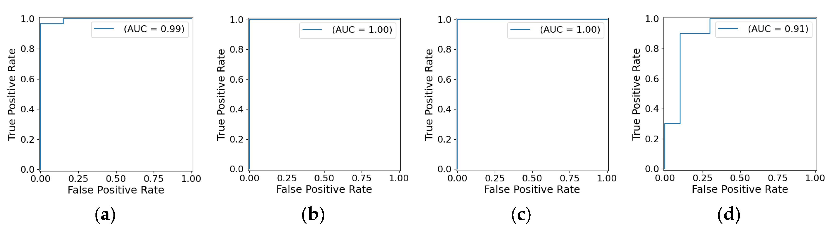
Figure 19.
Visualization of DCM, highlighting significant LV enlargement and reduced systolic function, accompanied by detailed metrics, including LV volumes, myocardial mass, ejection fractions, and wall thicknesses, to provide a comprehensive analysis of the pathological condition.
Figure 19.
Visualization of DCM, highlighting significant LV enlargement and reduced systolic function, accompanied by detailed metrics, including LV volumes, myocardial mass, ejection fractions, and wall thicknesses, to provide a comprehensive analysis of the pathological condition.
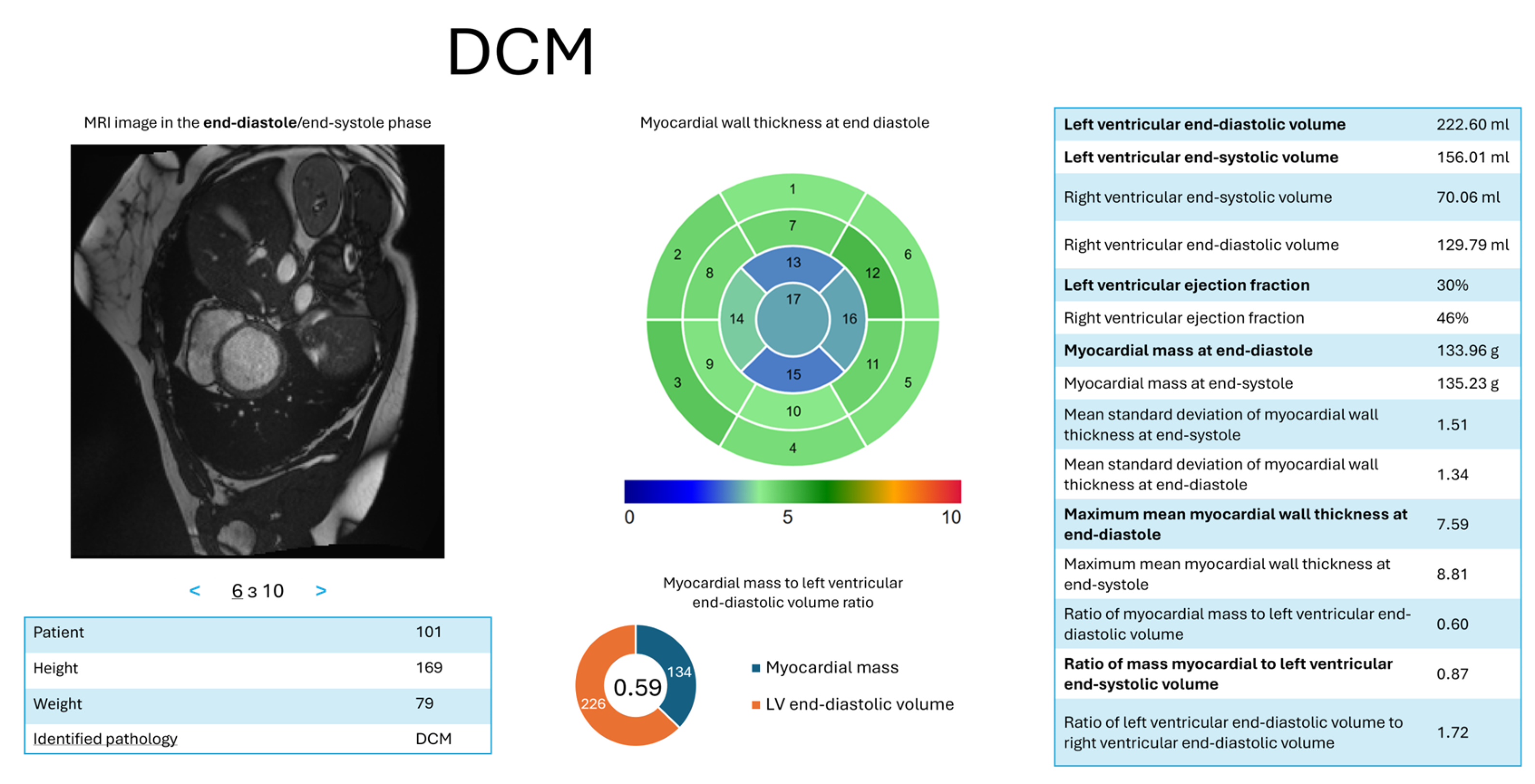
Figure 20.
Illustration of the impact of insufficient brightness on cardiac MRI analysis, where low brightness levels hinder the accurate delineation of cardiac structures, as shown in (a) the original image and (b) the myocardium segmentation (highlighted in yellow), leading to degraded model performance and poorly defined boundaries.
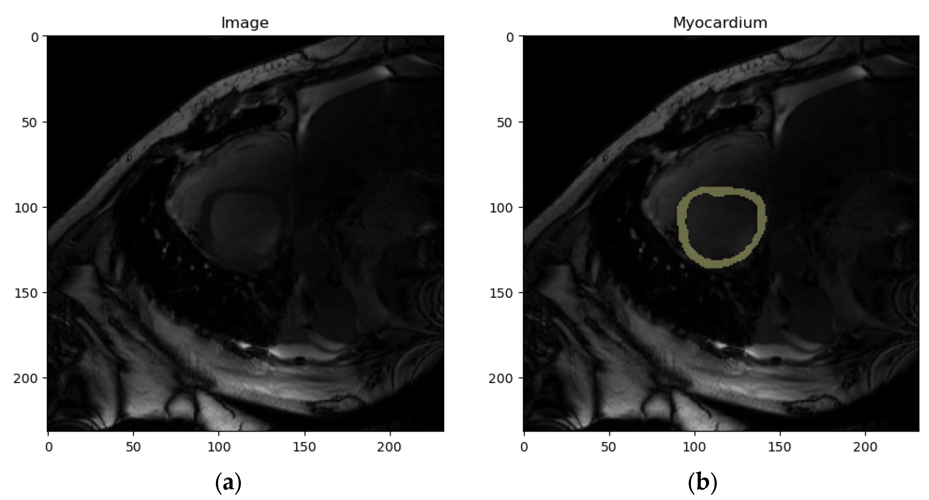
Figure 21.
Partial myocardium visualization challenges, as shown in (a) the original image and (b) the myocardium segmentation (highlighted in yellow), where the lower myocardium (marked in red rectangle) is poorly visible due to slice timing issues. Such incomplete visualizations may lead to inaccurate segmentation and train the model to erroneously fill missing areas.
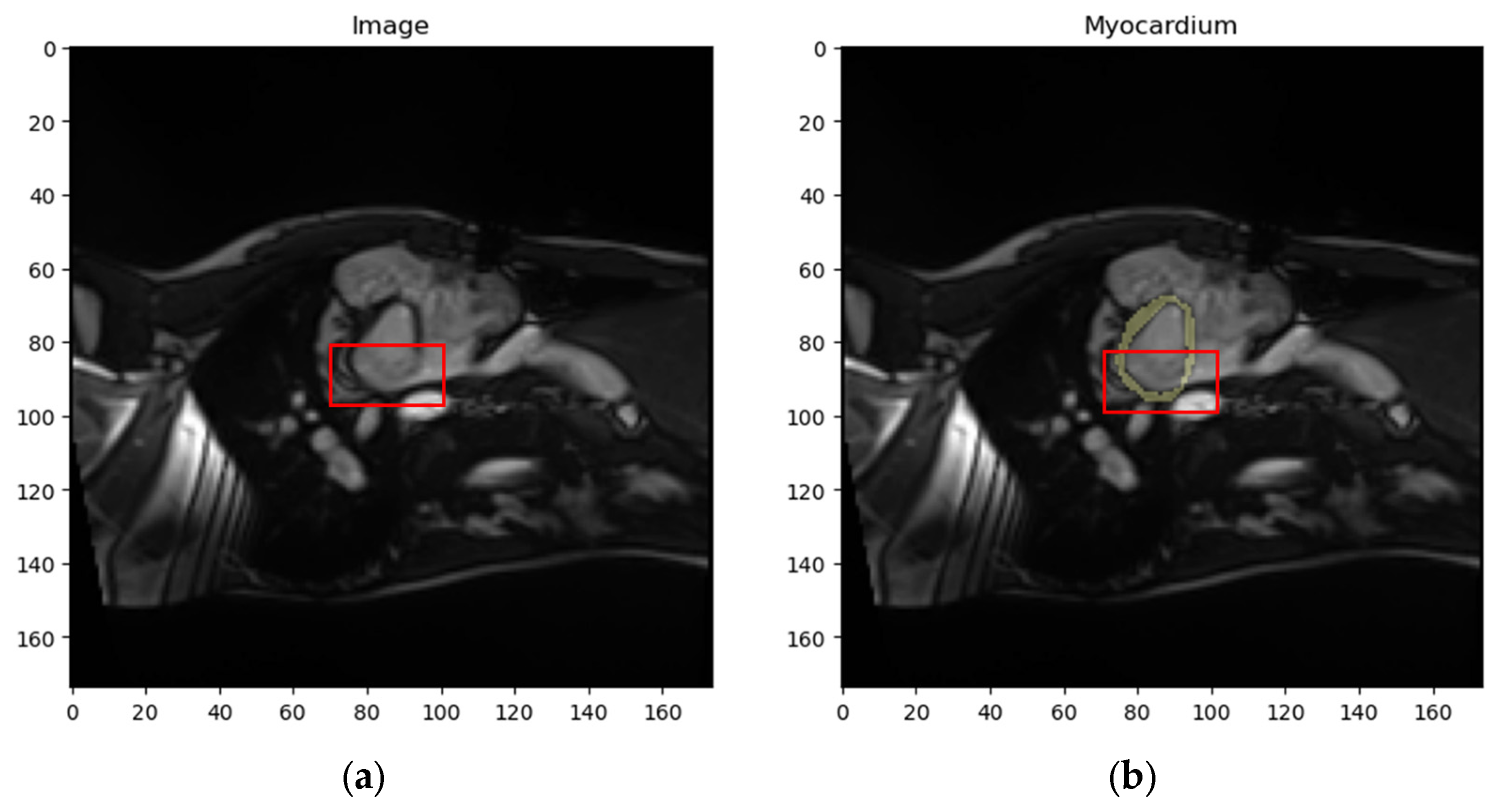

Table 1.
Results of the fifth experiment. Obtained mean Dice coefficient values for different segments. Numbers in bold show the highest scores.
Table 1.
Results of the fifth experiment. Obtained mean Dice coefficient values for different segments. Numbers in bold show the highest scores.
| Models | ED | ES | ||||
|---|---|---|---|---|---|---|
| LV | RV | Myocardium of the LV | LV | RV | Myocardium of the LV | |
| 0.911 | 0.842 | 0.812 | 0.890 | 0.871 | 0.832 | |
| , , , , , + postprocessing | 0.974 | 0.947 | 0.896 | 0.940 | 0.915 | 0.920 |
Table 2.
Computational results, i.e., Dice coefficient values, for evaluating the effectiveness of localization, decomposition, and postprocessing steps in the proposed segmentation method. Numbers in bold show the highest scores.
Table 2.
Computational results, i.e., Dice coefficient values, for evaluating the effectiveness of localization, decomposition, and postprocessing steps in the proposed segmentation method. Numbers in bold show the highest scores.
| Experiments | ED | ES | ||||
|---|---|---|---|---|---|---|
| LV | RV | Myocardium of the LV | LV | RV | Myocardium of the LV | |
| Experiment 1 | 0.911 | 0.842 | 0.812 | 0.890 | 0.871 | 0.832 |
| Experiment 2 | 0.920 | 0.902 | 0.875 | 0.894 | 0.891 | 0.884 |
| Experiment 3 | 0.919 | 0.892 | 0.855 | 0.887 | 0.873 | 0.885 |
| Experiment 4 | 0.956 | 0.939 | 0.866 | 0.930 | 0.905 | 0.898 |
| Experiment 5(proposed approach) | 0.974 | 0.947 | 0.896 | 0.940 | 0.915 | 0.920 |
Table 3.
Comparison of segmentation results with the state of the art using the Dice coefficient. Numbers in bold show the highest scores.
Table 3.
Comparison of segmentation results with the state of the art using the Dice coefficient. Numbers in bold show the highest scores.
| Works | ED | ES | ||||
|---|---|---|---|---|---|---|
| LV | RV | Myocardium of the LV | LV | RV | Myocardium of the LV | |
| Hu et al. [27] | 0.968 | 0.946 | 0.902 | 0.931 | 0.899 | 0.919 |
| da Silva et al. [28] | 0.963 | 0.932 | 0.892 | 0.911 | 0.883 | 0.901 |
| Ammar et al. [34] | 0.964 | 0.935 | 0.889 | 0.917 | 0.879 | 0.898 |
| Bourfiss et al. [35] | 0.959 | 0.929 | 0.875 | 0.921 | 0.885 | 0.895 |
| Ours | 0.974 | 0.947 | 0.896 | 0.940 | 0.915 | 0.920 |
Table 4.
Results of cardiologist’s analysis for myocardium masks, LV masks, and RV masks.
| Description | Number of marked samples | ||
|---|---|---|---|
| Myocardium masks | LV masks | RV masks | |
| Mask obtained by the proposed method has higher accuracy | 133 | 136 | 122 |
| Expert-annotated maskhas higher accuracy | 56 | 52 | 30 |
| Both masks have high accuracy, and the difference between masks is insignificant | 1976 | 1962 | 1959 |
| Both masks have low accuracy,insufficient for medical conclusions | 1 | 2 | 5 |
Table 5.
Classification evaluation metrics for Classifiers 1–4 were obtained at steps 1–4, respectively, within the proposed classification method.
Table 5.
Classification evaluation metrics for Classifiers 1–4 were obtained at steps 1–4, respectively, within the proposed classification method.
| Classifier | Classes | Precision | Recall | F1-score | Accuracy |
|---|---|---|---|---|---|
| Classifier 1 | NOR+ARV | 0.95 | 0.95 | 0.95 | 0.96 |
| MINF+HCM+DCM | 0.97 | 0.97 | 0.97 | ||
| Classifier 2 | NOR | 1.00 | 1.00 | 1.00 | 1.00 |
| ARV | 1.00 | 1.00 | 1.00 | ||
| Classifier 3 | HCM | 1.00 | 1.00 | 1.00 | 1.00 |
| MINF+DCM | 1.00 | 1.00 | 1.00 | ||
| Classifier 4 | MINF | 0.90 | 0.90 | 0.90 | 0.90 |
| DCM | 0.90 | 0.90 | 0.90 |
Table 6.
Comparison of classification results with state-of-the-art methods by overall accuracy. Numbers in bold show the highest scores.
Disclaimer/Publisher’s Note: The statements, opinions and data contained in all publications are solely those of the individual author(s) and contributor(s) and not of MDPI and/or the editor(s). MDPI and/or the editor(s) disclaim responsibility for any injury to people or property resulting from any ideas, methods, instructions or products referred to in the content. |
© 2025 by the authors. Licensee MDPI, Basel, Switzerland. This article is an open access article distributed under the terms and conditions of the Creative Commons Attribution (CC BY) license (http://creativecommons.org/licenses/by/4.0/).
Copyright: This open access article is published under a Creative Commons CC BY 4.0 license, which permit the free download, distribution, and reuse, provided that the author and preprint are cited in any reuse.


