Casting Light on Dependency Structures in Ensemble Forecasts with the 2-D Rank Histogram

1. Introduction

Multivariate forecasting involves predicting future values of multiple dependent variables simultaneously. By contrast, univariate forecasting only predicts a single variable’s future values. Bivariate forecasting is the simplest of the multivariate cases where only two variables are under focus at the same time. A physically consistent weather forecast is multivariate by nature with components in time (e.g. over the next hours or days), in space (e.g. for different locations), and across weather variables (e.g. wind and precipitation).

Nowadays, ensemble forecasts are the cornerstone of operational weather forecasting (Leutbecher and Palmer 2008). To optimise decision-making, forecast uncertainty is key not only with regard to a single variable at a given location and date but also across variables and time and space. In a multivariate framework, we are interested in this joint probability distribution between variables captured by an ensemble forecast. An assessment of the statistical consistency of multivariate forecasts is of practical interest from a forecast user perspective but also for forecast developers to identify deficiencies and pathways for improvement of their “multivariate forecast generator”.

The quality of multivariate ensemble forecasts can be assessed with the help of scores such as the Dawid-Sebastiani score or the p-variogram score (Dawid and Sebastiani 1999; Scheuerer and Hamill 2015). Another example is the energy score, a generalisation of the continuous ranked probability score. Weighted versions of multivariate scores have also been suggested recently (Allen et al. 2023). Nevertheless, verification results based on multivariate scores are sometimes difficult to interpret. In particular, univariate and multivariate contributions to the score are not easy to disentangle. Similarly, a separate assessment of the “reliability” and “resolution” components of a score is not straightforward. While recent studies discussed discrimination ability of multivariate forecasts with proper scores (Alexander et al. 2022; Pinson and Tastu 2013; Ziel and Berk 2019), others investigated the forecast reliability as discussed below. Reliability is a fundamental attribute for decision-making optimisation (e.g. Richardson 2011) and how to assess it in a multivariate context will be the main focus of this manuscript.

Tools for assessing the reliability of multivariate forecasts already exist such as, for example, multivariate rank histograms (Gneiting et al. 2008; Thorarinsdottir et al. 2014). Multivariate rank histograms are based on the computation of pre-ranks (Gneiting et al. 2008; Thorarinsdottir et al. 2014). Defining pre-ranks consists in finding a rank in a multivariate space by summarising a multivariate quantity into a single value. For example, average ranking assigns a pre-rank based on the average univariate rank as introduced in Thorarinsdottir et al. (2014). The complexity of the histogram interpretation in the multivariate case led to the recommendation of using several pre-ranking methods simultaneously to better understand the forecast miscalibration properties (Wilks 2017). Recently, Allen et al. (2024) suggested that the pre-rank function could be defined ad-hoc, to capture some relevant aspect of the multivariate forecast such as the mean, the variance, or the isotropy.

Here, we propose the use of a 2-D rank histogram applied to the bivariate case as an extension to the standard ensemble rank histogram. By contrast with previous works on multivariate rank histograms, the investigation takes place directly in the 2-D space rather than relying on a transformation to a 1-D space with the help of pre-ranks. The aim is to develop a tool for the visual inspection and assessment of dependency structures in bivariate ensemble forecasts. In the following, particular attention is paid to the visualisation of the histograms and their interpretation. Our study also introduces a new measure of ensemble reliability by summarising 2-D rank histograms into a single number. Although the focus here is on the simplest multivariate case, that is the bivariate case, a generalisation to more components would be straightforward.

This manuscript is organised as follows: in Section 2, we provide practical and technical descriptions of the rank histograms and how to build them; in Section 3, we discuss their visualisation and summary statistics; in Section 4, illustrations are based on a toy model while in Section 5 the tools are applied to real data before concluding in Section 6.

2. Rank Histograms

2.1. Schematically

Before developing a theoretical and practical framework for 2-D rank histograms, the topic is introduced with a schematic view of how 1-D (standard) and 2-D rank histograms can be constructed. Illustrations are provided in Figure 1 and Figure 2, respectively.

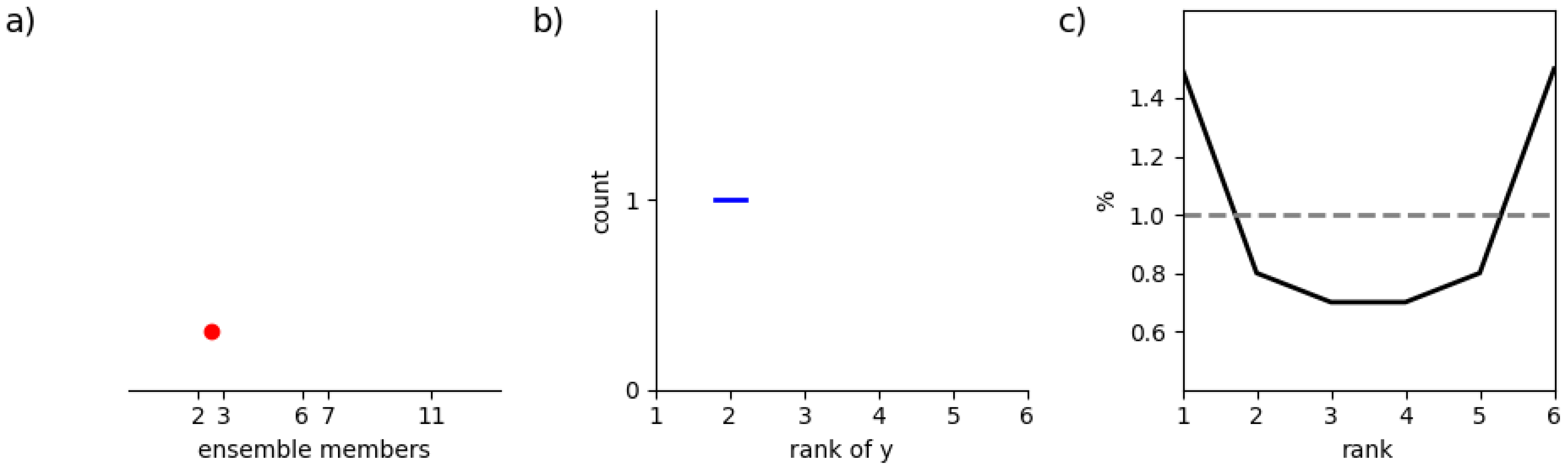
In Figure 1, we recall how a 1-D rank histogram is built. If we consider an ensemble forecast with members issuing values 2, 3, 6, 7, and 11 and an observation measuring 2.5 as represented in Figure 1(a), the rank of the observation is 2. So a count is added to this bin as in Figure 1(b). Repeating this operation over a verification sample, we obtain a histogram represented here as a line in Figure 1(c). The ideal 1-D histogram is flat with minor deviations due to sample noise as indicated by a dashed line.

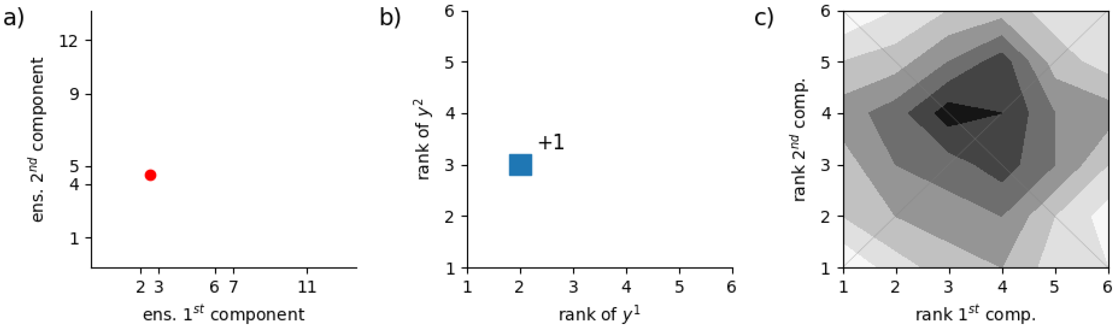
In Figure 2, we illustrate how rank histograms are built for 2-D ensemble forecasts. For the first component (variable), ensemble members and observation are the same as Figure 1, but here, we also consider a second component (variable) for which the ensemble members take values 1, 4, 5, 9, and 12 while the observation measures 4.5 as illustrated in Figure 2(a). The rank of the observation is 2 and 3 for the first and second components, respectively. The corresponding 2-D histogram bin is augmented by a unit Figure 2(b). After populating the rank histogram over the verification sample, we obtain a 2-D histogram as in Figure 2(c).

The ideal histogram is not know a-priori in the case of a 2-D rank histogram. So, to interpret Figure 2(c), one needs a reference. This reference varies on a case by case basis and can be obtained by representing the ensemble copula in the form of a 2-D histogram as discussed hereafter.

2.2. In Theory

2.2.1. In 1-D

Let’s consider a probability distribution function $\mathcal{F}$ and a sample from this distribution with M sorted elements $f^i$ with $i\in 1,...,M$. Also, let’s denote 2 fictive element $f^0$ and $f^{M+1}$ defined such that $\mathbb{P}(x<f^0)=0$ and $\mathbb{P}(x<f^{M+1})=1$, $\forall x$, respectively.

Consider an element g drawn from an unknown distribution $\mathcal{G}$. The probability of g having rank i among the M elements drawn from $\mathcal{F}$ is denoted $q\left(i\right)$. By definition, we have:

$$q\left(i\right):=\mathbb{P}(f^{i-1}<g<f^i),$$

(1)

for $i\in 1,...,M+1$. If the distributions $\mathcal{G}$ and $\mathcal{F}$ are identical, the probability distribution q is uniform. The elements $\mathcal{G}$ and $\mathcal{F}$ are in that case statistically indistinguishable.

2.2.2. In 2-D

Consider now that $\mathcal{F}$ and $\mathcal{G}$ are multivariate distribution functions, say bivariate for simplicity. We draw M elements from $\mathcal{F}$ and sort their 2 components separately ($f_1^i$ and $f_2^j$ with $i,j\in 1,...,M$) and draw one element from $\mathcal{G}$ with components $g_1$ and $g_2$. Similarly as for the univariate case, we consider the fictive elements $f_1^0$, $f_1^{M+1}$, $f_2^0$, and $f_2^{M+1}$ such that $\mathbb{P}(x_1<f_1^0)=0$, $\mathbb{P}(x_1<f_1^{M+1})=1$, $\forall x_1$, and $\mathbb{P}(x_2<f_2^0)=0$, $\mathbb{P}(x_2<f_2^{M+1})=1$, $\forall x_2$, respectively. In that case, the probability of $g_1$ being of rank i while simultaneously $g_2$ being of rank j is denoted $Q(i,j)$:

$$Q(i,j):=\mathbb{P}\left((f_1^{i-1}<g_1<f_1^i)\cap (f_2^{j-1}<g_2<f_2^j)\right),$$

(2)

for $i,j\in 1,...,M+1$.

In the case where $\mathcal{F}$ and $\mathcal{G}$ are identical, the resulting distribution Q is a discretized representation of the copula of the underlying multivariate distribution function. A copula describes the dependency structure between the components of the distribution that is, for example, wether one component being larger implies that the other component tends to be larger as well.

Recalling Sklar’s theorem (Sklar 1959), a bivariate distribution F of the random variable $v_1$ and $v2$ can be decomposed as:

$$F(v_1,v_2)=\mathcal{C}\left(F_{V_1}\left(v_1\right),F_{V_2}\left(v_2\right)\right)$$

(3)

where $F_{V_1}$ and $F_{V_2}$ are the univariate marginal distributions and $\mathcal{C}$ a copula function for the dependencies.The distribution function $\mathcal{C}$ is bivariate in this example, defined on the unit hypercube (that is defined on $[0,1]$ in all dimensions) and independent of the marginal.

2.3. In Practice

2.3.1. The Ensemble Rank Histogram

Consider an ensemble $\mathbf{e}$ with M members $e^i$, $i\in 1,...,M$ and the corresponding observation y. A rank histogram is built from the rank r of the observation with respect to the ensemble members:

$$r=\sum _{i=1}^M\mathbb{I}[y>e^i]+1$$

(4)

where $\mathbb{I}\left[x\right]$ is the indicator function taking value 1 if x is true, 0 otherwise, and with r taking value in $1,...,M+1$ and.

For reasons that will become clearer in the following, one can also build M rank histograms based on only $M-1$ ensemble members, eliminating one member of the ensemble at a time for each histogram. In that case, ranks are derived as:

$${\tilde{r}}^j=\sum _{i=1,i\ne j}^M\mathbb{I}[y>e^i]+1,$$

(5)

with ${\tilde{r}}^j$ taking value in $1,...,M$. The resulting M rank histograms denoted $H^j$ with $j\in 1,...,M$ are populated over N samples (that is pairs of ensemble forecast and observation). Each histogram category k is obtained as follows:

$$H_k^j=\sum _{n=1}^N\mathbb{I}\left[{\tilde{r}}^j=k\right],$$

(6)

for k in $1,...,M$ and where the index n is not added to the rank ${\tilde{r}}^j$ for readability. $H^j$ are "standard" rank histograms built with only $M-1$ ensemble members. The resulting averaged histogram is simply defined as:

$${\overline{H}}_k={\displaystyle \frac{1}{M}}\sum _{j=1}^M{H}_k^j,\forall k.$$

(7)

For each histogram of this kind, the ensemble member set apart can be used as a pseudo-observation. We denote c the rank of the pseudo-observation:

$$c^j=\sum _{i=1,i\ne j}^M\mathbb{I}[e^j>e^i]+1,$$

(8)

with j in $1,...,M$ for each of the ensemble member $e^j$. In other words, $c_j$ corresponds to the rank of member j within the ensemble. If we solve ties at random, $c_j$ takes a different value in $[1,...,M]$ for each $j\in 1,...,M$.

Similarly as for $H^j$, M pseudo-rank histograms $C^j$ are populated over N samples following:

$$C_k^j=\sum _{n=1}^N\mathbb{I}\left[c^j=k\right],$$

(9)

for k in $1,...,M$.

By averaging over all ensemble members, we obtain:

$${\overline{C}}_k={\displaystyle \frac{1}{M}}\sum _{j=1}^M{C}_k^j$$

(10)

and, by construction, we have:

$${\overline{C}}_k={\displaystyle \frac{N}{M}},\forall k.$$

(11)

In plain words, Eq. 11 states that the averaged pseudo-rank histogram is perfectly flat because it can’t be biased: each of the members contributes to its own ensemble in an unbiased way by definition. When considering observations, a rank histogram is flat up to sampling uncertainty when the observation is drawn from the same distribution as the ensemble. This interpretation is the basic interpretation of the ensemble reliability based on a rank histogram (Hamill and Juras 2006).

2.3.2. The 2-D Ensemble Rank Histogram

We now consider that both ensemble forecasts and observations have 2 components. In that case, a 2-D rank histogram is defined as a matrix H where each element $H_{k_1,k_2}$ corresponds to the number of cases where the bivariate observation $(y_1,y_2)$ is of rank $k_1$ along the first component and simultaneously of rank $k_2$ along the second component among the bivariate ensemble members ($e_1^i$,$e_2^i$) with $i\in 1,...,M$. Formally, we define the ranks as follows:

$$r_1=\sum _{i=1}^M\mathbb{I}[y_1>e_1^i]+1,r_2=\sum _{i=1}^M\mathbb{I}[y_2>e_2^i]+1$$

(12)

with $r_1$ and $r_2$ taking value in $1,...,M+1$.

Now, setting apart one member at a time as we did previously, we obtain M rank estimates for each component:

$${\tilde{r}}_1^j=\sum _{i=1,i\ne j}^M\mathbb{I}[y_1>e_1^i]+1,{\tilde{r}}_2^j=\sum _{i=1,i\ne j}^M\mathbb{I}[y_2>e_2^i]+1$$

(13)

and populate 2-D rank histograms as follows:

$$H_{k_1,k_2}^j=\sum _{n=1}^N\mathbb{I}\left[{\tilde{r}}_1^j=k_1\right]\mathbb{I}\left[{\tilde{r}}_2^j=k_2\right],$$

(14)

for $k_1$, $k_2$ in $1,...,M$. The averaged 2-D rank histogram (or simply 2-D rank histogram) is defined as:

$${\overline{H}}_{k_1,k_2}={\displaystyle \frac{1}{M}}\sum _{j=1}^M{H}_{k_1,k_2}^j\forall k_1,k_2.$$

(15)

Similarly, the 2-D rank histogram based on ensemble members used as pseudo-observations is derived from:

$$c_1^j=\sum _{i=1,i\ne j}^M\mathbb{I}[e_1^j>e_1^i]+1,c_2^j=\sum _{i=1,i\ne j}^M\mathbb{I}[e_2^j>e_2^i]+1$$

(16)

to build

$$C_{k_1,k_2}^j=\sum _{n=1}^N\mathbb{I}\left[c_1^j=k_1\right]\mathbb{I}\left[c_2^j=k_2\right],$$

(17)

for $k1$, $k2$ in $1,...,M$. The resulting averaged 2-D histogram based on pseudo-observations is a representation of the ensemble copula (simply referred to as ensemble copula in the following) and is defined as:

$${\overline{C}}_{k_1,k_2}={\displaystyle \frac{1}{M}}\sum _{j=1}^M{C}_{k_1,k_2}^j\forall k_1,k_2.$$

(18)

We can note that, by construction, $\overline{C}$ has the following property:

$$\sum _{k_1=1}^M{\overline{C}}_{k_1,k_2}={\displaystyle \frac{N}{M}}\forall k_2,$$

(19)

and

$$\sum _{k_2=1}^M{\overline{C}}_{k_1,k_2}={\displaystyle \frac{N}{M}}\forall k_1.$$

(20)

This result is equivalent to the one in Eq. (11): when aggregated to a 1-D rank histogram, this histogram based on pseudo-observations is by construction flat. This property is illustrated with 2 made-up examples below considering $N=1$, $M=5$ and showing the averaged histogram $\overline{C}$ times the ensemble size M:

$$\mathrm{example}1\text{:}\left[\begin{array}{ccccc}1& 0& 0& 0& 0\\ 0& 0& 0& 1& 0\\ 0& 0& 0& 0& 1\\ 0& 0& 1& 0& 0\\ 0& 1& 0& 0& 0\end{array}\right]$$

(21)

and

$$\mathrm{example}2\text{:}\left[\begin{array}{ccccc}0& 0& 0& 0& 1\\ 0& 0& 0& 1& 0\\ 0& 0& 1& 0& 0\\ 0& 1& 0& 0& 0\\ 1& 0& 0& 0& 0\end{array}\right].$$

(22)

With these 2 examples, we illustrate that the copula is a uniform multivariate distribution. In the copula, the row and column summations are flat, whereas in the 1-D case the histogram is flat when the ensemble is reliable. The 2-D topography of the copula reflects how both variables map to each other which can happen in many different ways

3. Multivariate Ensemble Reliability

3.1. Visualisation of 2-D Rank Histograms

For an ensemble of size M, the number of 2-D histogram categories (or bins) to be populated is $M^2$. When M is large, it can be difficult to estimate accurately the histogram distribution with a limited verification sample size. As a consequence, the estimated 2-D rank histogram and corresponding ensemble copula can appear noisy. As a noise reduction strategy, we recommend to aggregate adjacent categories to build a histogram of size $M^{\prime }\times M^{\prime }$ with $M^{\prime }$ a factor of M. For example, in the following, we use $M^{\prime }=5$ for an ensemble of size $M=50$. This choice of $5\times 5$ as a size for 2-D histograms is an empirical one. The optimal design in terms of categories as a function of the verification sample size is let for future investigations.

The noise reduction by aggregation of categories allows the visualisation of simpler patterns that ease their interpretation. For this reason, we recommend 2-D rank histograms to be visualised in the form of aggregated histograms. This strategy is applied in the following.

3.2. Summary Scores

The visual comparison of a 2-D rank histogram $\overline{H}$ and the corresponding ensemble copula $\overline{C}$ helps identify deficiencies in an ensemble forecasting system. We provide examples based on synthetic data and ECMWF ensemble forecasts in Section 4 and Section 5, respectively. However, it is also often useful to summarise rank histograms in a single number that reflects the ensemble performance in terms of reliability. In the univariate case, 2 measures of histogram goodness (flatness) are commonly used: the $\delta$-score (Candille and Talagrand 2005) and the the reliability index ($RI$, Delle Monache et al. 2006.

RI and $\delta$-score differ in the error metric used to measure the distance between a rank histogram and the expected histogram for a perfect system, namely the absolute and square error, respectively. If we consider a univariate rank histogram with elements $H_k$, $k\in 1,\dots ,M+1$ for an ensemble of size M, build over N cases, and with $p_k$ the probability of an observation to fall in category k for a perfect system, we have the following definitions:

$$RI(H,Np)=\sum _{k=1}^{M+1}|H_k-N{p}_k|$$

(23)

and

$$\Delta (H,Np)=\sum _{k=1}^{M+1}{\left(H_k-N{p}_k\right)}^2$$

(24)

with $\Delta$ a building block of the $\delta$-score. In the case of a univariate ensemble forecast, the probability $p_k$ is known a-priori and is equal to ${\displaystyle \frac{1}{M+1}}$ for all categories k of the histogram.

A generalisation to the multivariate case requires considering that the probability1 $p_{k_1,k_2}$ in case of a reliable system is well approximated up to a constant by the ensemble copula $\overline{C}$. Based on this assumption, we can reformulate $\Delta$ in the multivariate case as follows:

$$\Delta (H,C)=\sum _{j=1}^M\sum _{k_1=1}^M\sum _{k_2=1}^M{\left(H_{k_1,k_2}^j-{\overline{C}}_{k_1,k_2}\right)}^2,$$

(25)

for $j\in 1,\dots ,M$. Note that here, $\Delta$ is computed for each individual 2-D rank histogram $H^j$ separately. A generalisation of $RI$ would follow the same reasoning but is not discussed here further.

In (Candille and Talagrand (2005), the $\delta$-score is defined as $\Delta$ normalised by ${\Delta }_0$, the expected value of $\Delta$ in case of a reliable forecast. In our setting, ${\Delta }_0$ can be derived from the histograms $C^j$ build from pseudo-observations:

$${\Delta }_0\left(C\right)=\sum _{j=1}^M\sum _{k_1=1}^M\sum _{k_2=1}^M{\left(C_{k_1,k_2}^j-{\overline{C}}_{k_1,k_2}\right)}^2,$$

(26)

Eventually, we suggest the following definition of the $\delta$-score for multivariate rank histograms:

$$\delta (H,C)={\displaystyle \frac{\sqrt{\Delta (H,C)}}{\sqrt{{\Delta }_0\left(C\right)}}},$$

(27)

with the use of square roots that has been added here with respect to the original definition in the univariate case. A $\delta$-score close to one is interpreted as an indication that the 2-D ensemble forecast is reliable. A $\delta$-score (significantly) higher than 1 is interpreted as an indication that there is a reliability issue in the ensemble forecast, while a $\delta$-score (significantly) lower than one “would indicate that the successive realizations of the prediction process are not independent” (Candille and Talagrand 2005).

3.3. Disentanglement

One of the main drawbacks of existing measures of performance designed for multivariate forecasts is the complexity of their interpretation. In particular, it is often difficult to distinguish between contributions from univariate miscalibration (biases and spread biases) and contributions from mis-specifications in the dependency structure of the forecast components (too strong or too weak correlation between variables, for example). A method to disentangle these two contributions is suggested here.

Our approach relies on transforming 2-D rank histograms $H^j$ into marginally adjusted 2-D rank histograms, denoted ${\tilde{H}}^j$. The idea is to mimic the impact of a univariate statistical post-processing step on rank histograms by moving elements of $H^j$ to obtain a 2-D histogram with the desirable properties while preserving the dependence structure. Post-processing refers here to methods that correct for systematic errors in the forecast. When effective, post-processing leads to a forecast statistically consistent with the observations. Hence, one expects a flat 1-D rank histogram (up to sample variations) after univariate post-processing.

The transformation of a 2-D rank histogram $H^j$ into an adjusted 2-D rank histogram ${\tilde{H}}^j$ consists in enforcing that the sum of ${\tilde{H}}^j$ along both of its components follow a uniform-like distribution while maintaining the existing dependence structure between components. Let’s denote $\mu$ the target uniform histogram and $\nu$ the 1-D rank histogram derived by aggregating $H^j$ along one of its components. An optimal transport algorithm is used to find how to move elements of $\nu$ to obtain $\mu$ with a minimal “displacement” effort. The adjusted 2-D histogram ${\tilde{H}}^j$ is obtained by enforcing these displacements for the one component while keeping the distributions of the other component unchanged. Technical details of this approach are provided in Appendix A.

By construction, the histograms ${\tilde{H}}^j$ have the characteristics of a system perfectly calibrated for each component separately but still depict the original dependency structure. For plotting purposes, we average the adjusted 2-D rank histograms ${\tilde{H}}^j$ and denote the resulting histogram simply $\tilde{H}$. As for H, one can visualise $\tilde{H}$ and compare it with the ensemble copula $\overline{C}$. Also, following Eq. 27, one can compute the $\delta$-score for adjusted rank histograms.

4. Toy-Model Experiments

4.1. Settings

A toy model is used to provide illustrative examples of 2-D rank histograms when reliability deficiencies are simulated in a controlled environment. The toy model is built as follows. The simulated observations y are drawn from a bivariate normal distribution:

$$y_{1,2}\sim \mathcal{N}(\mathit{\mu },\mathbf{\Sigma })\mathrm{with}\mathit{\mu }=\left[\begin{array}{c}0\\ 0\end{array}\right]\mathrm{and}\mathbf{\Sigma }=\left[\begin{array}{c}{\sigma }^2\rho {\sigma }^2\\ \rho {\sigma }^2{\sigma }^2\end{array}\right]$$

(28)

with ${\sigma }^2$ the variance and $\rho$ the correlation between the 2 components. To simulate some variability in the variance of the observation distribution, $\sigma$ is drawn from a uniform distribution : $\sigma \sim \mathcal{U}(0.8,1.2)$. Similarly, the variability in the strength of the correlation between the two variables is simulated by drawing the correlation coefficient $\rho$ from a uniform distribution $\rho \sim \mathcal{U}(0.6,0.8)$.

The simulated ensemble consists in forecasts $e^j$, $j\in 1,\dots ,M$, draw from a bivariate normal distribution such that

$$e_{1,2}^j\sim \mathcal{N}(\mathit{\mu },\mathbf{\Sigma })\mathrm{with}\mathit{\mu }=\left[\begin{array}{c}ϵ\\ ϵ\end{array}\right]\mathrm{and}\mathbf{\Sigma }=\left[\begin{array}{c}\alpha {\sigma }^2\beta \rho \alpha {\sigma }^2\\ \beta \rho \alpha {\sigma }^2\alpha {\sigma }^2\end{array}\right]$$

(29)

where the parameters $ϵ$, $\alpha$, and $\beta$ can be modified to simulate different types of miscalibration. It is worth pointing out the symmetry in this setting (the bias affects both components identically, for example) which is usually not the case in real applications (different biases for the 2 components). The forecast is drawn from the same bivariate normal distribution as the observations when $ϵ=0$, $\alpha =1$, and $\beta =1$. The set of experiments and corresponding parameter combinations used for illustration are indicated in Table 1. For all experiments, we set $M=50$ and $N=50000$.

4.2. Results

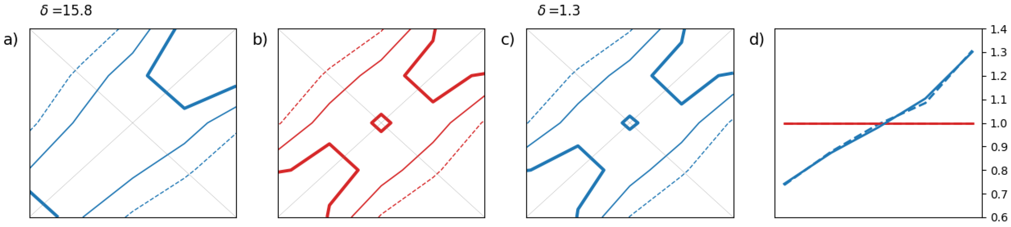
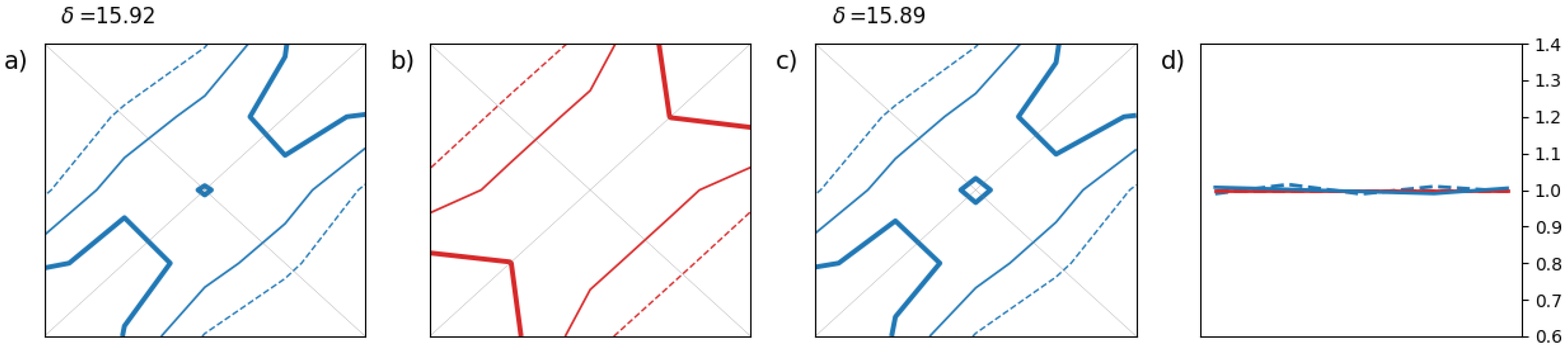
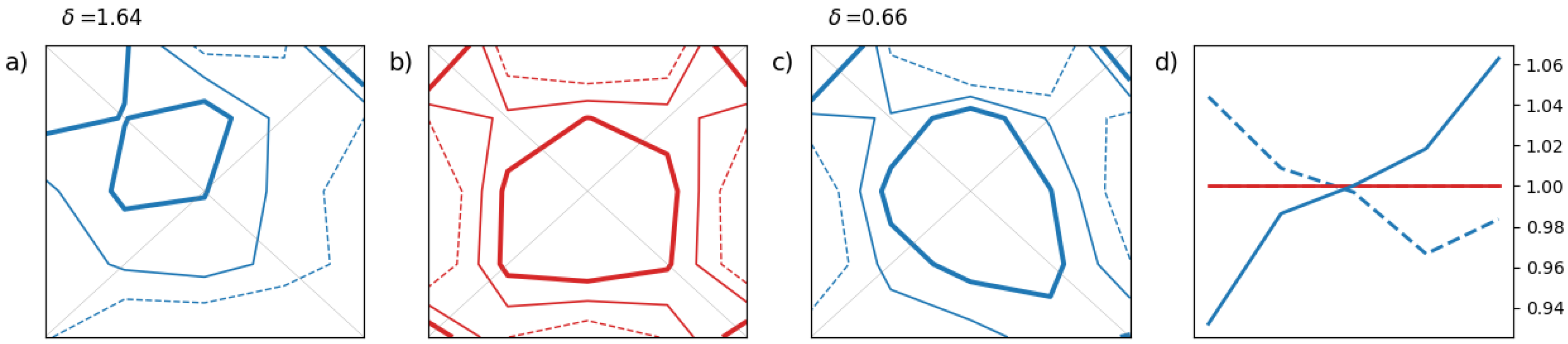
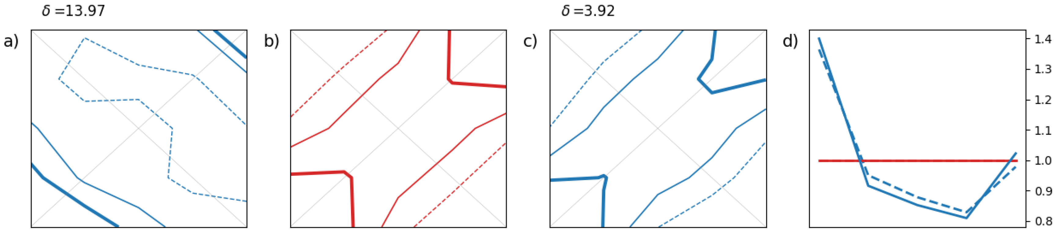
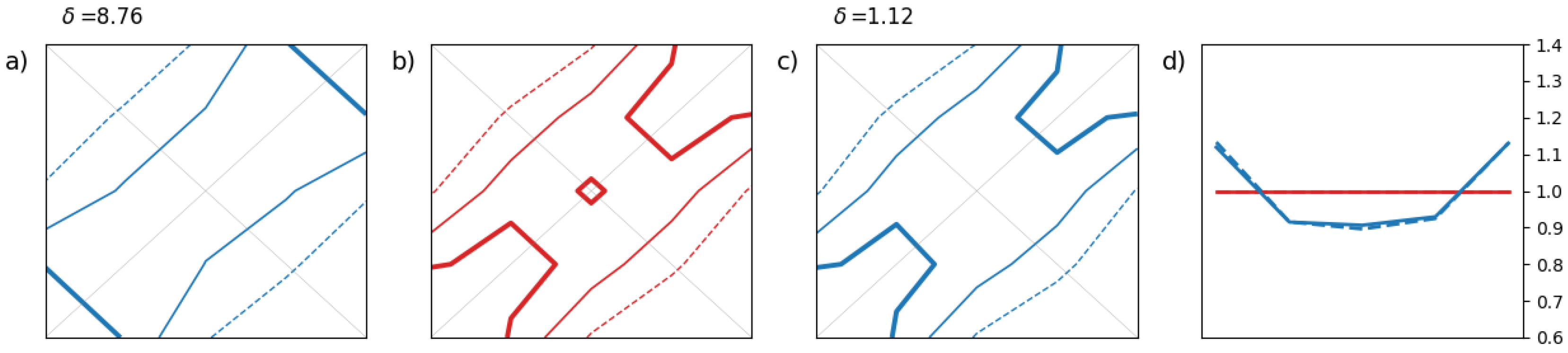
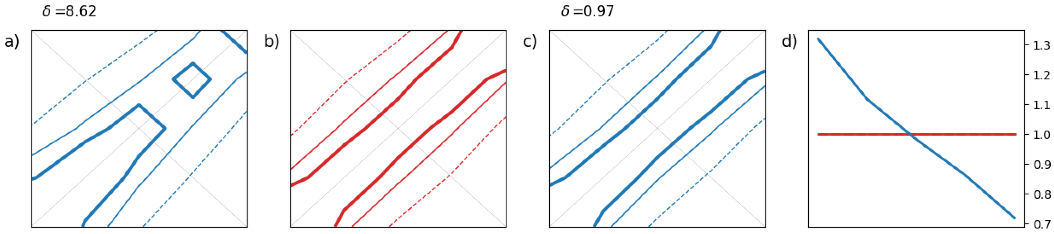
The first illustrative example in Figure 3 shows the impact of a bias on the rank histograms. The second example in Figure 4 simulates a lack of spread among ensemble members. The third example in Figure 5 shows the impact of a too-weak correlation between the 2 components of the ensemble. For each example, the 2-D rank histogram $\overline{H}$ in (a) is compared with the estimated ensemble copula $\overline{C}$ in (b). We also show the adjusted 2-D rank histogram $\tilde{H}$ in (c) and univariate rank histograms for both components in (d).

These simple examples help to associate basic patterns or shapes with common miscalibration features. A bias in the forecast leads to a 2-D histogram which is tilted as in Figure 3(a) while a lack of spread in the ensemble results in a 2-D histogram depleted in its center as in Figure 4(a). In these 2 cases, the marginal distributions are affected by a miscalibration but not the dependency between components. In that case, we observe that, after adjustment, the 2-D rank histograms in Figure 3(c) and Figure 4(c) match reasonably well the ensemble copulas in Figure 3(b) and Figure 4(b), respectively. Also, we recover the standard results for the univariate case as shown in Figure 3(d) and Figure 4(d): the classical L- and U-shape for biased and underdispersive forecasts, respectively.

The third synthetic example focuses on a dependency structure issue in the ensemble forecast. The forecast is perfectly calibrated in a univariate sense. For this reason, Figure 5(a) and Figure 5(c) are almost identical because the adjustment has no impact on the already well-calibrated 2-D histogram, and the 1-D rank histograms are close to flatness in Figure 5(d). Also, the $\delta$-score is unaffected by the histogram adjustment in this example as the ensemble is already well calibrated marginally.

In the third synthetic example, the flaw in the dependency structure of the ensemble is revealed when comparing the ensemble copula in Figure 5(b) with 2-D histograms in Figure 5(a) or Figure 5(c). The ensemble copula appears more populated towards the lower left and upper right corners than the 2-D histograms which are more populated along the diagonal, especially at the center. It is worth noting that 2-D rank histograms can take various shapes depending on the covariance structure of the data and the calibration property of the forecasting system. This variety is difficult to grasp here with a small number of examples.

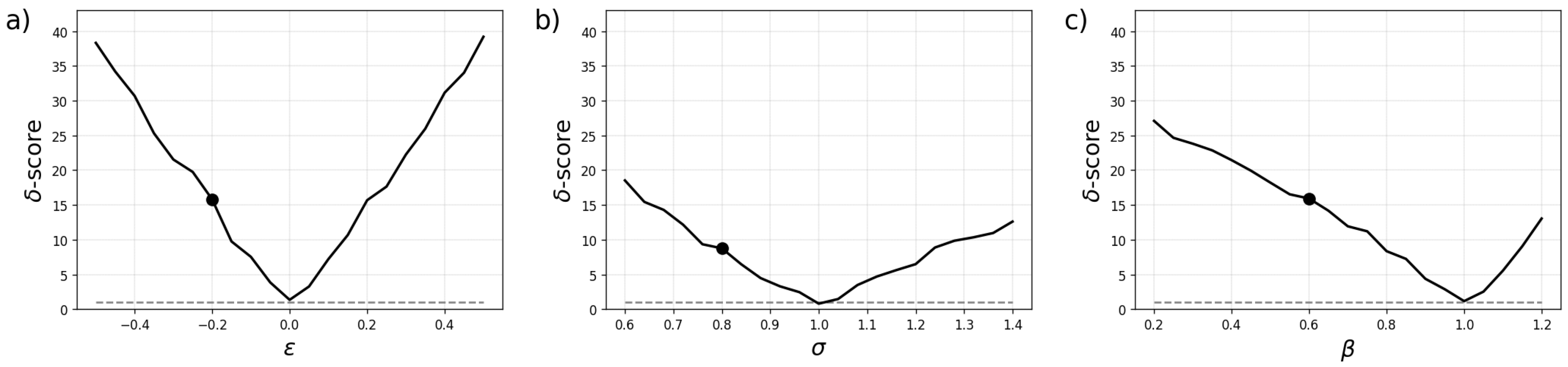
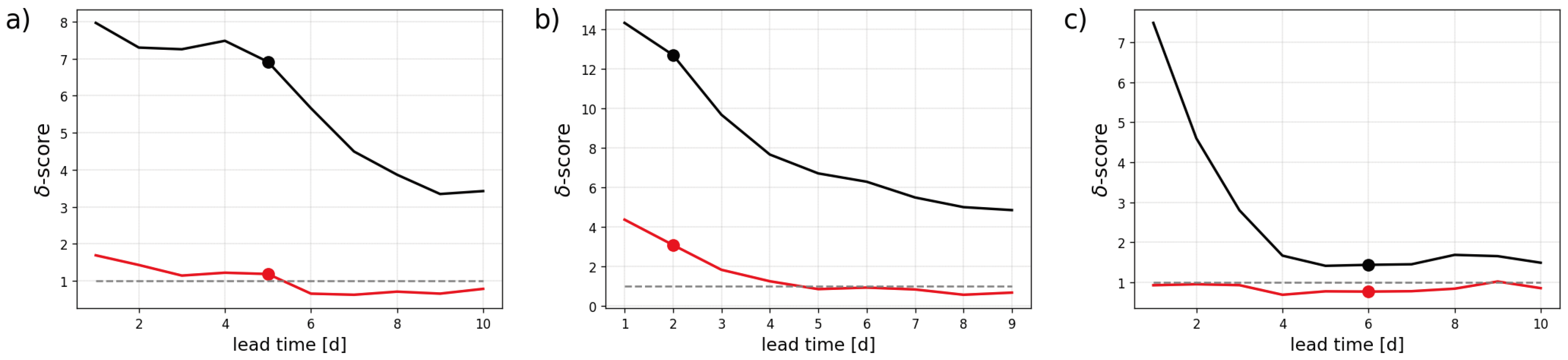
Finally, Figure 6 illustrates how the $\delta$-score varies when one of the parameters of the toy model is changed at a time. The optimal value for the $\delta$-score is 1, indicating multivariate forecast reliability. This minimum is reached, as expected, when the parameters are set to $ϵ=0$, $\sigma =1$, and $\beta =1$ corresponding to the case where forecasts and observations are drawn from the same bivariate distribution. These plots reveal that the $\delta$-score is particularly sensitive to deviations in marginal miscalibration due to a bias in the forecast as in Figure 6(a) than a miscalibration in terms of the dependencies as in Figure 6(c). This result illustrates further the importance of disentangling marginal calibration from dependency miscalibration otherwise errors in terms of a bias would tend to dominate reliability performance measures.

5. Application to ECMWF Ensemble Forecasts

5.1. Data and Settings

We now apply the concept of 2-D rank histogram to the ensemble run at ECMWF. We choose examples that capture different types of bivariate forecasts with components in space, time, or between variables. The 3 examples are the following: 1) geo-potential height forecasts at 500hPa (Z500) shifted spatially in a zonal direction, 2) temperature forecasts at 850hPa (T850) at 2 different lead times, and 3) wind components, zonal and meridional, at 200hPa. For each forecast component, the verifying ECMWF analysis is used as “observation”. So, for example, when a forecast is shifted spatially, we use a shifted analysis as observation. The different configurations are reported in Table 2.

For illustration purposes, forecasts are compared to observations at a 1.5° spatial grid resolution. In our examples, the verification period covers March 1 to May 31 (MAM) 2024. The focus in on the Northern Hemisphere which counts approximately 5700 grid points. The ensemble size is 50.

5.2. Results and Discussion

In the first real example in Figure 7, we assess visually Z500 ensemble forecasts. A bivariate forecast is build here from 2 forecasts of the same variables but (zonally) distant by $3^{\circ }$, in practice by 2 grid points. The statistical consistency of the ensemble with the observations is assessed by comparing the 2-D rank histogram in Figure 7(a) with the ensemble copula in Figure 7(b). The former appears tilted with respect to the latter indicating a bias in the forecast as in the synthetic example in Figure 3. This interpretation is corroborated by the 1-D rank histogram in Figure 7(d). In this example, both components have the same 1-D rank histogram as they correspond to the same forecast shifted spatially. Furthermore, the adjusted 2-D histogram in Figure 7(c) matches the ensemble copula in Figure 7(b) with a $\delta$-score close to 1. This result is interpreted as follows: the spatial dependency in the ensemble is well-calibrated for this example.

The second example in Figure 8 shows results for T850 with a focus on the temporal consistency of the ensemble. A bivariate forecast corresponds indeed to 2 forecasts of the same variable but at 2 consecutive lead times. In Figure 8(a), the 2-D histogram appears depleted in its center indicating a miscalibration of the ensemble spread similarly as in the synthetic example in Figure 4. The under-dispersiveness of the ensemble is further confirmed by the 1-D rank histograms in Figure 8(d). More interestingly, we note a slight discrepancy between the ensemble copula in Figure 8(b) and the adjusted histogram in Figure 8(c): the latter tends to be more populated along the diagonal than the former. Supported by the synthetic example in Figure 5(b) and Figure 5(c), this result is interpreted as a too-weak correlation between ensemble members at consecutive lead times in that case.

As a third real example, Figure 9 shows rank histograms for the wind forecast components at 200hPa. The 2-D pattern of the ensemble copula in Figure 9(b) indicates a mix of positive and negative correlation among ensemble members: all the corners are reasonably populated as well as the centre of the 2-D histogram. We see a similar pattern after adjustment of the 2-D rank histogram as shown in Figure 9(c). The $\delta$-score is in that case below 1. The ensemble dependency in the wind components seems well calibrated. The main reliability issue detected here is related a positive bias in the meridional component and a negative bias in the zonal one as picked up by the 1-D rank histograms in Figure 9(d).

Finally, in Figure 10, the $\delta$-score is plotted as a function of the forecast lead time for the 3 types of bivariate forecasts analysed above. The summary measure of ensemble reliability is computed not only for 2-D rank histograms but also for their adjusted versions. The adjustment that mimics the impact of a univariate postprocessing helps decrease the $\delta$-score significantly: the major contribution to the score originates from bias and ensemble spread miscalibration. The reliability score is close to 1, or even below 1, in most of the cases after adjustment of the histograms. One notable exception is for T850 forecasts at shorter lead times as shown in Figure 10(b).

6. Summary and Outlook

A new diagnostic tool is designed to gain insights into the ability of ensemble forecasts to provide reliable information not only in a univariate sense (for one variable, one lead time, and one location) but also in a multivariate framework. The 2-D rank histogram is a generalisation of the popular ensemble rank histogram to the situation where the focus is on 2 variables simultaneously rather than just one. The simplest multivariate case offers an appealing framework for approaching and assessing ensemble reliability when the number of forecast components is greater than one.

In the univariate case, the rank histogram for a reliable forecast is expected to be flat. In the bivariate case, the shape of the 2-D histogram for a reliable forecast is not known beforehand but rather should match the dependency structure between the 2 components of the ensemble forecast. This shape differs on a case by case basis. For this reason, a 2-D rank histogram needs to be compared with an estimation of the ensemble copula which represent this dependency structure. The estimation of the ensemble copula is based on a leave-one-member-out approach, where the left-out member is used as a pseudo-observation to build the reference histogram.

The visual inspection of a 2-D rank histogram and its comparison with the corresponding ensemble copula helps identify miscalibration issues in ensemble forecasts. First, we generate synthetic datasets and associate 2-D patterns with common pathological forecasts such as a biased forecast, a lack of ensemble spread, or a too-weak correlation between components of the ensemble. Similar patterns are then easy to interpret when observed in 2-D rank histograms derived from real data. In our study, we diagnose ECMWF ensemble forecasts for various variables and settings. Besides the expected biases and underdispersivnes issues, we also found that the ensemble shows good reliability in terms of dependency structures, except between consecutive forecasts of T850 at shorter lead times.

In addition, we introduce a summary statistic of the 2-D rank histogram, the $\delta$-score, which provides a way to measure ensemble reliability in a multivariate space. The $\delta$-score formulated in this paper is inspired by a similar score for 1-D rank histogram. We also suggest using an optimal transport algorithm to adjust 2-D rank histograms to “virtually” correct the ensemble for systematic univariate miscalibration. The histogram adjustment is a way to disentangle different sources of miscalibration and focus on the dependency structure in the ensemble.

The rank histogram appears as a versatile tool that can be easily applied to bivariate ensemble forecasts. In principle, the concept of rank histogram could be generalised to more than 2 components. The visualisation of such histograms would effectively be challenging for a number of forecast components greater than 2 or 3. However, the $\delta$-score would still be a simple mean to assess the ensemble reliability in the defined multivariate space. The histogram aggregation step that combines adjacent histogram categories to improve robustness (and reduce noise) would be even more crucial in that case. The optimal number of histogram categories and, more generally, statistical testing of 2-D rank histograms is left for future work.

References

- Alexander, C., M. Coulon, Y. Han, and X. Meng, 2022: Evaluating the discrimination ability of proper multi-variate scoring rules. Ann Oper Res. [CrossRef]
- Allen, S., J. Bhend, O. Martius, and J. Ziegel, 2023: Weighted verification tools to evaluate univariate and multivariate probabilistic forecasts for high-impact weather events. Weather and Forecasting, 38 (3), 499–516. [CrossRef]
- Allen, S., J. Ziegel, and D. Ginsbourger, 2024: Assessing the calibration of multivariate probabilistic forecasts. Quarterly Journal of the Royal Meteorological Society, 150 (760), 1315–1335. [CrossRef]
- Candille, G., and O. Talagrand, 2005: Evaluation of probabilistic prediction systems for a scalar variable. Quarterly Journal of the Royal Meteorological Society, 131 (609), 2131–2150. [CrossRef]
- Dawid, A. P., and P. Sebastiani, 1999: Coherent dispersion criteria for optimal experimental design. The Annals of Statistics, 27 (1), 65 – 81. [CrossRef]
- Delle Monache, L., J. P. Hacker, Y. Zhou, X. Deng, and R. B. Stull, 2006: Probabilistic aspects of meteorological and ozone regional ensemble forecasts. Journal of Geophysical Research: Atmospheres, 111 (D24). [CrossRef]
- Gneiting, T., L. I. Stanberry, E. P. Grimit, L. Held, and N. A. Johnson, 2008: Assessing probabilistic forecasts of multivariate quantities, with an application to ensemble predictions of surface winds. Test, 17, 211–235. [CrossRef]
- Hamill, T. M., and J. Juras, 2006: Measuring forecast skill: is it real or is it the varying climatology? Quart. J. Roy. Meteor. Soc., 132, 2905–2923. [CrossRef]
- Leutbecher, M., and T. N. Palmer, 2008: Ensemble forecasting. Journal of computational physics, 227 (7), 3515–3539.
- Pinson, P., and J. Tastu, 2013: Discrimination ability of the energy score. Technical report, Technical University of Denmark.
- Richardson, D. S., 2011: Economic value and skill. Forecast Verification: A Practitioner’s Guide in Atmospheric Science, I. T. Jolliffe, and D. B. Stephenson, Eds., John Wiley and Sons, 167–184.
- Scheuerer, M., and T. M. Hamill, 2015: Variogram-based proper scoring rules for probabilistic forecasts of multivariate quantities. Mon. Wea. Rev., 143, 1321–1334. [CrossRef]
- Sklar, M., 1959: Fonctions de répartition à n dimensions et leurs marges. Publ. Inst. Statist. Univ. Paris, 8, 229–231.
- Thorarinsdottir, T., M. Scheuerer, and C. Heinz, 2014: Assessing the calibration of high-dimensional ensemble forecasts using rank histograms. arXiv, 2303.17195. [CrossRef]
- Virtanen, P., R. Gommers, T. E. Oliphant, M. Haberland, T. Reddy, D. Cournapeau, E. Burovski, and al, 2020: SciPy 1.0: Fundamental Algorithms for Scientific Computing in Python. Nature Methods, 17, 261–272. [CrossRef]
- Wilks, D. S., 2017: On assessing calibration of multivariate ensemble forecasts. Quarterly Journal of the Royal Meteorological Society, 143 (702), 164–172. [CrossRef]
- Ziel, F., and K. Berk, 2019: Multivariate forecasting evaluation: On sensitive and strictly proper scoring rules. arXiv. [CrossRef]