MNIST Dataset Heatmap Classifier

1. Introduction

Traditional image analysis methods required a complicated process of manual feature extraction. Thanks to convolutional networks, we got rid of this problem. They have revolutionized image recognition tasks in many key aspects, which has had a huge impact on the development of artificial intelligence. They are adapted to process large sets of visual data, are sufficiently resistant to translations or noise. CNNs have found applications not only in image recognition, but also in other fields, such as sound analysis, text analysis, genomics, as well as in new technologies such as speech recognition, video analysis or emotion recognition based on facial expressions.

One of the first deep convolutional networks is LeNet (LeCun et al., 1998). It was successful in the task of recognizing handwritten digits. It was a pioneer in the application of CNNs to image recognition; despite its limited computational resources and small number of parameters, it provided a foundation for further research on deep convolutional networks. The AlexNet architecture (Krizhevsky et al., 2017) was also a breakthrough achievement that contributed to the rapid growth of popularity of convolutional networks. This architecture was presented in the context of the ImageNet competition, where it achieved a revolutionary result, reducing the classification error by more than 10% compared to previous methods.

Alternative methods for classifying digits from the MNIST set have already been used, such as Variational AutoEncoder (Mak, Han & Yin, 2023), which achieved 85.4% accuracy, Neuromorphic Nanowire Networks with 97.8% accuracy (Zhu et al., 2021), or even the Cellular Automata mechanism for self-classifying digits (Levin et al., 2020). I propose to use the simplest heatmap in the form of averaging the values of all training data, and for classification purposes calculating how similar the image is to that map. The results of an exemplary implementation for recognizing digits from the MNIST set (LeCun, Cortes & Burges, 1994), which contains 60,000 training images and 10,000 testing images, were evaluated.

2. Classifier Design

2.1. Structure

To correctly construct the classifier, a heatmap must be initialized for each class i as a zero matrix of dimensions $n\times m$.

$$X_i=\left[\begin{array}{cccc}0& 0& \cdots & 0\\ 0& 0& \cdots & 0\\ ⋮& ⋮& \ddots & ⋮\\ 0& 0& \cdots & 0\end{array}\right]\mathrm{where}{X}_i\in {\mathbb{R}}^{n\times m}$$

After training the classifier on the selected samples, each matrix should already have specific values.

$$X_i=\left[\begin{array}{cccc}{x}_{11}& x_{12}& \cdots & x_{1m}\\ x_{21}& x_{22}& \cdots & x_{2m}\\ ⋮& ⋮& \ddots & ⋮\\ x_{n1}& x_{n2}& \cdots & x_{nm}\end{array}\right]\mathrm{where}{X}_i\in {\mathbb{R}}^{n\times m}$$

Next, to determine which class assign the tested sample to, you need to evaluate how well it fits each class. This means calculating the absolute value of the deviation of the image p from the heatmap x, so for each pixel j, we calculate

$$P_j=\left|p_j-x_j\right|$$

We calculate the $\mathcal{K}$ index (assuming that 255 is the maximum pixel value) to determine how well the image fits the selected class

$${\mathcal{K}}_i={\displaystyle \frac{{\sum }_{j=1}^{nm}(255-P_j)}{255nm}}$$

Choose the one with the highest $\mathcal{K}$ index, without using additional activation functions. It’s index is the result of which class should be assigned to an image.

2.2. Training

To update the zero matrix, we should calculate the average over all training samples S, where s is the number of such samples

$$X_i={\displaystyle \frac{{\sum }_{j=1}^s{S}_j}{s}}$$

We update the value of the selected heatmap, preserving a number representing the total number of samples $\mathcal{A}$ it was trained on.

$$X_i\leftarrow {\displaystyle \frac{X_i*\mathcal{A}+{\sum }_{j=1}^s{S}_j}{\mathcal{A}+s}}$$

2.3. Time Complexity

Assuming that the number of classifier samples is finite, all samples are known at the beginning and the amount of pixels is constant, training the classifier is achievable in $O\left(n\right)$, knowing n is the number of images. The evaluation of the classifier results will always be $O\left(1\right)$, because the number of classes and heatmaps is constant.

For example, feedforwarding of one layer of a convolutional neural network has time complexity $O\left(C_{in}{C}_{out}{K}^2\right)$, assuming that $C_{in}$ is the number of input channels, $C_{out}$ is the number of output channels and K is the filter size, which makes the time complexity of classifier evaluation much superior.

3. Classifier Variants

After training the baseline model on 60,000 samples from the MNIST dataset, it achieved just 66.85% correct matches on 10,000 test samples. Nevertheless, this is a very impressive result for a model that is not a convolutional network or even any kind of deep network.

In this paper, different variants will be discussed in order to obtain the best possible results.

Figure 1. Trained heatmaps of the standard variant

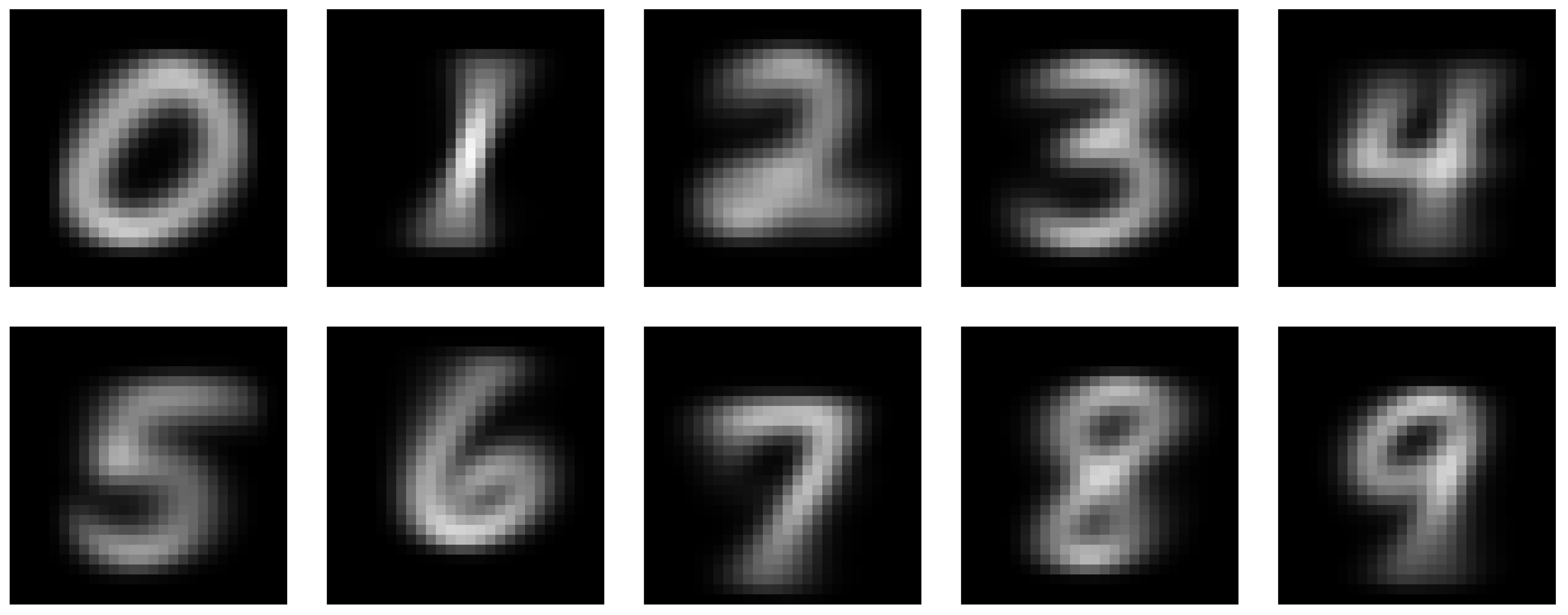
Figure 1. Trained heatmaps of the standard variant

3.1. No Zeros Variant

This model assumes that only pixels whose value is greater than zero will be used for heatmap update and classifier evaluation. Assuming that k is the number of pixels such that $p_j>0$, the index $\mathcal{K}$ should be normalized as follows

$$\begin{array}{c}{\mathcal{K}}_i=\sum _{\begin{array}{c}j=0\\ p_j>0\end{array}}^{nm}{\displaystyle \frac{255-\left|p_j-x_j\right|}{255k}}\end{array}$$

Figure 2. Trained heatmaps of the no zeroes variant

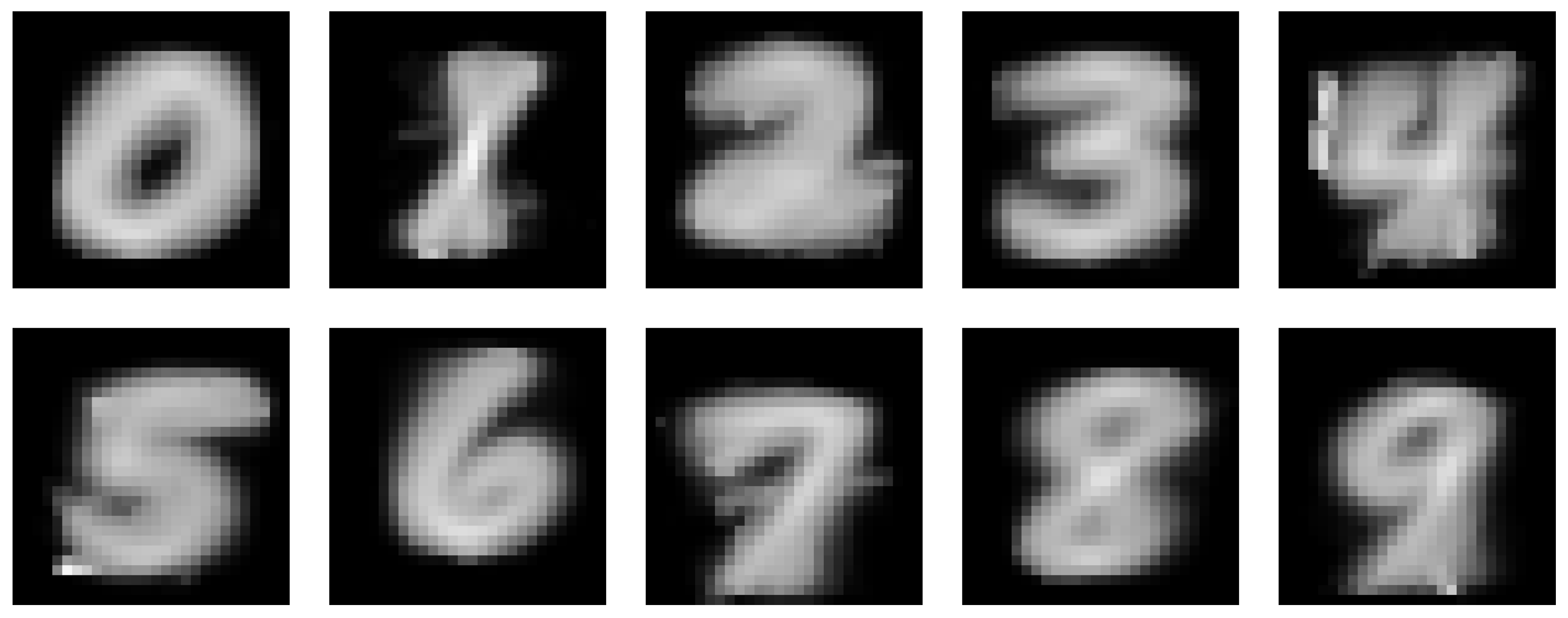
Figure 2. Trained heatmaps of the no zeroes variant

3.2. Adjusting Variant

Adjusting variant involves cutting out the region of interest from the sample and then scaling it to constant dimensions. By region of interest, we mean the smallest possible rectangle bounded by non-zero pixel values most prominent in each direction.

Figure 3. The process of extracting ROI and interpolating

Figure 3. The process of extracting ROI and interpolating

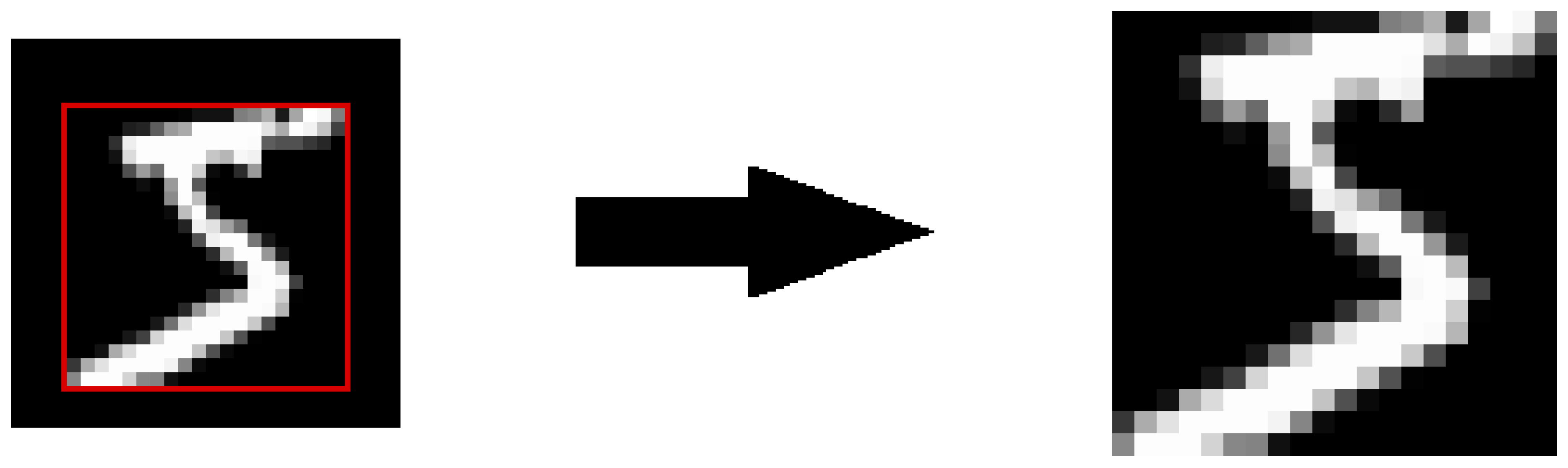
Then, the cut sample fragment must be resized to fixed dimensions. In the case of this work, nearest neighbor interpolation was implemented due to its simplicity and computational speed, and the heatmaps have fixed dimensions of 32x32 which were determined empirically.

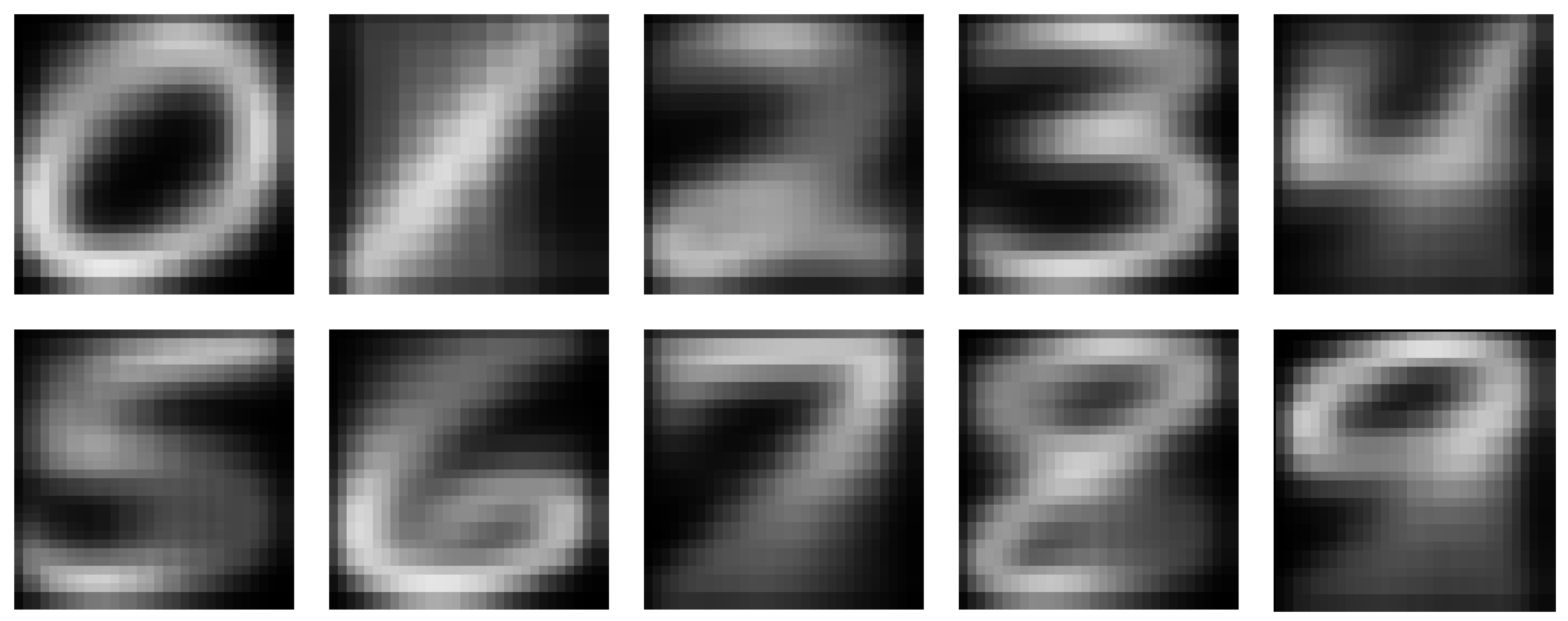
Figure 4. Trained heatmaps of the adjusting variant

Figure 4. Trained heatmaps of the adjusting variant

3.3. Adjusting Variant with Exponential $\mathcal{K}$ Index

To emphasize the importance of matching, we can exponentially increase the difference in error between the sample pixel and the heatmap.

$${\mathcal{K}}_i={\displaystyle \frac{{\sum }_{j=1}^{nm}({255}^k-P_j^k)}{{255}^{k}nm}}$$

Increasing the difference in deviation allows to give a larger impact factor to pixels that have the same value and to give a much smaller impact factor to pixels with extreme values. In this work, an empirical value of $k=3$ was found which gave measurably good results.

3.3.1. Simple Enhancement

Table 1 in the Adjusting enhanced section presents the results for the variant in which all heatmap pixel values were increased by 10%.

$$X_i\leftarrow max(1.1X_i,255)$$

Table 1. Results of MNIST classification.

	Accuracy in testing data	Accuracy in training data
Standard variant	66.85%	65.1$\overline{3}$%
No zeros variant	77.17%	76.195%
Adjusting standard	77.74%	76.20$\overline{3}$%
Adjusting exponential $\mathcal{K}$	80.78%	79.77%
Adjusting enhanced	81.31%	80.20$\overline{3}$%

Table 1. Results of MNIST classification.

	Accuracy in testing data	Accuracy in training data
Standard variant	66.85%	65.1$\overline{3}$%
No zeros variant	77.17%	76.195%
Adjusting standard	77.74%	76.20$\overline{3}$%
Adjusting exponential $\mathcal{K}$	80.78%	79.77%
Adjusting enhanced	81.31%	80.20$\overline{3}$%

4. Results

Each classifier was trained on the same samples from the MNIST dataset.

The difference in results between the standard model and the no zeros variant is primarily due to the amount of information stored in the heatmaps. Comparing the heatmap visualizations (Figure 1 and 2), you can see that no zeroes variant’s heatmaps are more complete and have a greater ability to match similarly shaped digits.

The adjusting variant allows to achieve similar accuracy as the no zeros variant, however it has an important advantage - universality. By interpolating the cropped to the region of interest samples we get a classifier that preserves the most important information about a given object such as shape or saturation of individual pixels and normalizes them to a common resolution. This solution could potentially expand classifier’s domain to other dataset, e.g. DIDA (Kusetogullari, Yavariabdi, Hall, & Lavesson, 2021).

5. Discussion and Conclusions

Adjusting variant achieves 81.31% accuracy, which translates into an error of 18.69%. This is an impressive result considering the training time, time complexity, space complexity and simplicity of implementation. I believe that this classifier has great potential and could achieve much higher accuracy if properly combined with convolutional networks. Combining several of the techniques mentioned in the paper in a different way can also positively influence the result. Unlike a neural network, this architecture allows us to completely bypass problems related to the gradient, computational efficiency and, above all, problems with the interpretation of results.

As a research direction in this area, I propose to analyze the results of training with data augmentation such as shearing, skewing, rotating or edge enhancement. In addition, classifiers on heatmaps can be combined with other machine learning methods - for example, the basic k-Nearest Neighbor algorithm achieved 96.91% accuracy on the MNIST dataset (Yepdjio Nkouanga & Vajda, 2023), so combining it appropriately with heatmaps classifiers could lead to better results.

References

- An, S.; Lee, M.; Park, S.; Yang, H.; So, J. An ensemble of simple convolutional neural network models for MNIST digit recognition. arXiv 2020. [Google Scholar] [CrossRef]
- Krizhevsky, A.; Sutskever, I.; Hinton, G. E. ImageNet classification with deep convolutional neural networks. Communications of the ACM 2017, 60(6), 84–90. [Google Scholar] [CrossRef]
- Kusetogullari, H.; Yavariabdi, A.; Hall, J.; Lavesson, N. DIGITNET: A deep handwritten digit detection and recognition method using a new historical handwritten digit dataset. Big Data Research 2020, 100182. [Google Scholar] [CrossRef]
- Kusetogullari, H.; Yavariabdi, A.; Hall, J.; Lavesson, N. DIDA: The largest historical handwritten digit dataset with 250k digits. June 2021. Available online: https://github.com/didadataset/DIDA/.
- Levin, M.; Greydanus, S.; Niklasson, E.; Randazzo, E.; Mordvintsev, A. Self-classifying MNIST digits. Distill 2020, 5. [Google Scholar] [CrossRef]
- LeCun, Y.; Cortes, C.; Burges, C. J. MNIST handwritten digit database. AT&T Labs. 1994. Available online: http://yann.lecun.com/exdb/mnist.
- Mak, H. W. L.; Han, R.; Yin, H. H. F. Application of variational autoencoder (VAE) model and image processing approaches in game design. Sensors 2023, 23(7), 3457. [Google Scholar] [CrossRef]
- Yepdjio Nkouanga, H.; Vajda, S. Optimization strategies for the k-nearest neighbor classifier. SN Computer Science 2023, 4(47). [Google Scholar] [CrossRef]
- Zhu, R.; Loeffler, A.; Hochstetter, J.; Diaz-Alvarez, A.; Nakayama, T.; Stieg, A.; Gimzewski, J.; Lizier, J. T.; Kuncic, Z. MNIST classification using neuromorphic nanowire networks. International Conference on Neuromorphic Systems 2021. [Google Scholar] [CrossRef]
Disclaimer/Publisher’s Note: The statements, opinions and data contained in all publications are solely those of the individual author(s) and contributor(s) and not of MDPI and/or the editor(s). MDPI and/or the editor(s) disclaim responsibility for any injury to people or property resulting from any ideas, methods, instructions or products referred to in the content. |
© 2025 by the authors. Licensee MDPI, Basel, Switzerland. This article is an open access article distributed under the terms and conditions of the Creative Commons Attribution (CC BY) license (http://creativecommons.org/licenses/by/4.0/).
Copyright: This open access article is published under a Creative Commons CC BY 4.0 license, which permit the free download, distribution, and reuse, provided that the author and preprint are cited in any reuse.