Submitted:
13 January 2025
Posted:
14 January 2025
You are already at the latest version
Abstract
This paper proposes novel approach to 3D virtual modeling of articulated mechanisms. It follows widespread use of XML for various applications and defines a version of XML specially designed for description of 3D geometric models of articulated bodies. It was shown how the 3D geometric model of a mechanism can be gradually developed using suitable defined elements and stored in corresponding XML file. The developed XML model is processed and using powerful VTK (Visualization Toolkit) library the corresponding virtual model is built and shown on the computer screen. To drive the virtual model the dynamical model of the mechanism is developed using Bond Graph modelling techniques. The models, 3D virtual geometric and dynamic, are created using the corresponding software packages: BonSim3D Visual and BondSim. The models are interconnected by a two-way named pipe. During the simulation of dynamical model, the parameters necessary to drive the virtual model (e.g., the joint displacements) are collected and sent to the virtual model over the pipe. When the virtual model receives a package the computer screen is updated showing the new state of the mechanism. The approach was demonstrated on example of a holonomic omnidirectional mobile robot.
Keywords:
3D visualization
; XML
; Omnidirectional mobile robot
; Path planning
; Bond Graphs
1. Introduction
With development of 3D CAD technologies, the visualization of processes and systems has become a powerful tool and has been increasingly used in process of the new products and processes design, providing numerous benefits such as shorter development time and smaller costs, the possibility of testing and verification of the functionality before the product production, checking of possible part collisions in space, comparison of different product and process solutions to choose an optimal one, etc.
The idea of remote access to the information of automatic systems and their visual representation appeared with the invention of the Internet. Following [1] the online approaches are proposed for remote control of automatic systems based on synchronous and asynchronous capabilities to control developed 3D models using XML (eXtensible Markup Language) technology. Many researchers have developed simulators with visual programming environments for the development, validation and optimization of various products and processes.
The role of simulators becomes extremely important in robotics as robotic systems are increasingly complex with numerous built-in sensors and complex tasks that the robots have to perform. The design, analysis, performance optimization, and navigation of robots in unstructured environments can greatly simplified using software for modeling and visualization.
In the last couple decades, many researchers have developed different software for simulation and visualization of the robot applications, which have obtained popularity and play important role in solving the engineering problems. Some of the widely used simulators for development of mobile robot applications are Gazebo [2,3] based on Robot Operating System (ROS) [4,5], Rviz—3D visualization tools for ROS [6], Webots [7,8], MORSE [9], CoppeliaSim [10,11], CARLA [12], Raisim [13], MARS (Multi-Agent Robot Simulator, developed in Matlab) [14], CARMEN (the Carnegie Mellon Navigation Toolkit) [15], MoveIt [16], etc.
To choose the right simulator for the development of a specific robot application among the widely developed ones, many investigators offer an overview of the most used 3D robotic simulators and evaluate their properties [17,18,19,20,21]. Some authors pointed out as powerful tools for modelling and visualization of the complex systems the Virtual Reality (VR) [22], Augmented Reality (AR) [23] and Mixed Reality (MR) [24]. Some useful algorithms for modeling and visualization of robots in Matlab are presented in [25].
This paper proposes a novel approach for 3D geometric modeling of articulated mechanisms, based on a version XML [26]. The main idea is to provide connection between such developed virtual model to its dynamic model, created using other software [27]. Two-ways communication between two models has established using named pipe technology.
The proposed approach is applied on an example of mobile robot FESTO Robotino [28]. Generally, the popularity of mobile robots is significantly growing in recent years and attracts the research attention around the world. On other hand, FESTO Robotino is complex enough to be chosen as a representative example. It is characterized by excellent maneuverability achieved using three omnidirectional wheels. As such, it is the subject of many analyzes presented in [29,30,31,32,33,34,35,36]. Generally, the construction of omnidirectional wheels is also given great attention and is the subject of research [37,38,39,40].
The dynamic models for various mobile robots have been developed several decades ago, but due to the complexity of omnidirectional wheels [31,32,33,34,35], the attention of researchers around the world is still focused on dynamic modeling and the design of an appropriate control algorithms for navigation of mobile robots equipped with such wheels [41,42,43].
In this paper, the lateral rolling of the rollers, which the wheels consist of, was taken into account and analyzed. Dynamic model, based on the concept of component model approach, has been created by bond graph technique using program BondSim [27,44].
The virtual 3D model of Robotino is developed in the paper using an XML approach by BondSim3DVisual application. Methodology for development of the virtual model presented here is updated, modified and conceptually different version of one explained in [45]. The proposed markup language is a simplification of general XML scheme found elsewhere [26] and serves as a replacement of a C-type language introduced in BondSim3DVisual [27]. The proposed version was designed for 3D geometric modeling of articulated bodies such as robots, multi finger robot hands, mobile robots, multi legs platforms, cranes and similar objects. Using a DOM (Document Object Model) like approach, an XML document can be represented as a tree of elements. Thus, the structure of 3D geometric model of an articulated mechanisms can be represented as a tree of constitutive elements and attributes in the computer memory. 3D virtual model is generated from XML tree using powerful VTK library [46,47,48].
Between two robot models: the virtual, which works in environment of BondSim3DVisual, and the dynamic model, which runs in BondSim, there exists two-way communication during simulation based on named pipe techniques. After validation in virtual environment, the proposed algorithms could be applied to a real robot. Verification of the robot’s behavior in a virtual scene reduces the need for large experimental work with real robots.
FESTO has implemented similar idea for Robotino using two software packages RobotinoView for driving of the Robotino, and RobotinoSim to visualize robot scene [49,50]. The approach presented in this paper is more general and refers to the development of dynamic and 3D virtual models of any articulated mechanism, not only Robotino. Such models can exchange information with each other in the planned future research on the real physical systems according to the concept of digital twins.
The rest of the paper is organized as follows. The methodology of how to develop a virtual 3D model of articulated mechanism is described in Section 2. The dynamic model of Robotino using bond graphs is developed in Section 3. Simulation results are presented in Section 4. Finally, the last part of the paper gives concluding considerations and proposes for the future work.
2. Virtual 3D Modelling of Articulated Mechanisms
2.1. The Basic Approach
The visualization in 3D space provides representing of three-dimensional objects on the computer screen similarly as we see them in the real scene. In the real scene we have several essential items (Figure 1):
- Three-dimensional space with objects in it;
- Sources of the light such as Sun, or light bulbs, enlightening the scene;
- A person looking at it.
The objects generally are not static, but move over the scene, e.g., a robot hand moves over the scene to grasp a part and moves it to another object to place or insert it there. We analyze their motion in world space OXYZ. We assume that XY plane lies in the plane where objects lie and we look to them along negative Z axis.
To visualize the objects and their movement over the scene, we
- generate virtual 3D representation of them as 3D geometric objects;
- generate dynamic model of the entire system in order to simulate their motion;
- interconnect these two worlds, 3D geometric and dynamical, by suitable means to enable interactions between them.
2.2. Generating Virtual 3D Model
To generate 3D virtual model of an articulated mechanism BondSim3DVisual application was developed using Microsoft Visual C++ language. It is used for construction of the 3D virtual model of a mechanisms and its generation on the computer screen. It uses a special version of Extensible Markup Language (XML). The application uses well known pugixml library [51] to support processing of XML code.
At opening of the application an empty mainframe appears, as shown in Figure 3. It is divided into two parts. On the left side there are two tabbed windows: Tree View and XML Output. The first one serves for construction of Document Object Model (DOM) like XML model tree. Thus, the model is not developed as a conventional XML document, but as DOM like tree. It starts at a root, and suitable elements and attributes are inserted one after other as its branches or leaves. Simultaneously, a corresponding XML document is generated in read-only XML Output window. To see it we simply click its title (Figure 3). The right side of the program frame is used to create a document window containing the virtual 3D objects corresponding to the XML model on the left.
The problems treated by this application are divided in several groups: projects, robots, tools and objects. This division is rather arbitrary and serves to define the roots of the model trees and the directories where their XML documents are stored. The models are stored as XML files, i.e., text files with extension XML.
From modelling and visualization point of view, Robots, Tools and Objects are all treated in the same way. Thus, when we need to develop a new robot model, e.g., 3D model of Robotino using BondSim3DVisual application we need to assign a unique name to the model, which is used as the filename for storing generated XML document in the Robot directory. We may select simply Robotino as the file name. Program starts by creating the robot tree root and adding the attributes as children (Figure 4a). The attribute id represents the robot identifier. It is a machine generated a unique number as shown in Figure 4b. The Name attribute contains Robotino textual value.
The operations on the tree are very simple. Starting from the root we insert elements or attributes by selecting a corresponding node (an element or attribute) by clicking it by mouse and applying Edit menu command, or right clicking it by the mouse. A drop-down menu appears from which an element or attribute can be chosen (Figure 5a) to insert. Another drop-down menu now appears from which a suitable command can be selected either to insert a new item as child, or above, or below of the selected item. The menu disappears and a dialog window appears from which an element or attribute node can be selected (Figure 5b). After selecting and clicking OK, the dialog closes and the selected item appears in the tree. The structure of the virtual model is generated systematically starting at the robot root and adding hierarchically its branches (elements) and leaves (attributes) following the structure of the mechanism we model.
Generating of the scene on the computer display is the responsibility of the computer graphic subsystem, which consists of display hardware, graphics hardware and graphic library. It is possible to program the graphic subsystem directly by use of the corresponding languages such as OpenGL, DirectX, etc. However, many applications use a suitable application library to simplify this task. To that purpose, the BondSim3DVisual uses the VTK, a powerful C++ library [46,47,48].
By applying Create 3D Scene command, the XML model description is processed and the corresponding virtual model frame is created at the right side of the application’s frame windows.
2.3. Modeling Articulated Mechanism
A typical articulated mechanism consists of a base (link 0) and series of body links connected by the joints. To describe mechanism, we use different coordinate frames. Thus, we add to every of body links an orthogonal coordinate system, which is fixed to the particular body link. There are two coordinate systems which are associated with every joint, and having the common origins. One of these frames is fixed to the previous link, and the other to the next link (Figure 6a). The relative position of these frames can be described by a common joint axis and a rotation angle/ translational displacement by which one joint frame displaces with respect to (w.r.t.) the other.
Figure 6a shows simple case of revolute joint. To define the next link coordinate frame defined by the corresponding rotation matrix, we start from the current frame rotation matrix and apply the pre-transforms to transform it to overlap the current joint frame fixed to the current link. These transforms usually consist of the translation which move the origin of the current link frame to the origin of the joint frames and rotation of the translated frames to align with the joint frame, which is fixed to the current frame. Next a drive transform is applied, which typically consists of a rotation or translation of the other joint frame around/along the joint axis. Finally, we apply post-transform, which align the other joint frame with the next link body frame. These transforms can be compactly described by XML tree segment shown in Figure 6b.
Often transforms along the body links are much simpler. Thus, e.g., joint coordinate frame fixed to the previous link can be used simultaneously as the link frame. In that case, pre- and post-transforms are not necessary (they are identity transforms); only the drive transform is needed.
After the rotation matrix of the next link frame is defined by above transforms, we need to describe the geometry of the next link. We may use different geometric elements such as cuboids, cones, cylinders, bodies of revolution e.t.c. for this purpose. All such elements are the children of the next joint, and thus they use as the reference frame the frame of the next body link, which id defined by the link element in Figure 6b. Hence, all of these elements have to follow the link element. Every of these elements have a unique id attribute, which is used to refer to them.
There is a special element—assembly. It is used it to add the geometric elements to it by referring to them by their ids. In this way all of the next body link geometric elements can be referred to as unit by the assembly id attribute. We can also use it to transform position and orientation of added elements w.r.t. the reference frame.
The articulated mechanism’s parts typically have the complex shapes and are usually generated using a 3D CAD software (e.g., SolidWorks, Catia etc.) [51,52], from which they can be exported in the form of STL files. This is the case with many robots including the Robotino. In this way the 3D virtual models of such robots can be reconstructed so that they are very close to the real devices. The main difference is in the color of the robot parts, because they are not defined in STL files; they contain the geometry data only. The corresponding stl files are specified by the part elements.
The final element in the joint segment is the render element. The element is inserted at the same level but below all body elements or assemblies it refers to. It connects geometry of the element or assemblies it refers to with the visualization object (the actor). It also connects to the link frame (the next body frame). Because the geometry does not contain information on the color, it is defined here. The color can be defined by a color name, similarly as in the web browsers (Edge, Google. etc.), or by the red, green or blue (RGB) color indices in range 0.0-1.0. This value is set to the color of the current visualization object.
2.4. Modeling of FESTO’s Omnidirectional Mobile Robot Robotino
The Robotino is an omnidirectional device, which has ability to move over the ground floor in any direction no matter what are the current orientations of theirs wheels (Figure 7). This is mainly result of the special design of the wheels. For version of Robotino studied in this paper, every wheel consists of two groups of three rollers each, which are contained in a wheel holder (supporter) in which they can rotate. The rollers in one group, e.g., the front or back group, are angularly displaced by 60⁰ w.r.t. the other in such a way that (looking at the wheel’s outer circle at the point of contact with the ground) the end of a roller of the first group overlaps the start of the roller of the other group. In this way, during the rotation of a wheel, at every moment one roller is in the contact with the ground floor and rolls over it. The coordinate system shown in the Figure 7a is the world coordinate system in which the device is described. It is displaced in order not to overlap the device. The Robotino consists of chassis and three wheels, which are displaced around the vertical axis by 120⁰. The wheels are driven by DC motors, which are connected to wheel axles by tooted belts and planetary gears. The basic parts of Robotino are shown in Figure 7b.
Figure 8 shows a scheme of Robotino with the local coordinate frames defined. There are three frames with the origins at the wheel centers Ci (i = 1,2,3) and whose xi axes (i = 1,2,3) are directed along the wheel rotation axes. We also added another local frame whose x-axis is directed opposite to x2 axis and serves to orient the Robotino. Their zi and z axes are parallel with the world Z axis; the yi and y axes are created by rotating xi and x axes around zi and z axes for 90⁰ in positive (counter clock wise ccw) sense. The local coordinate frames are fixed to Robotino chassis, and moves jointly with it.
We create a new virtual model of Robotino as explained in Section 2.2 (Figure 4). It generates the corresponding the robot root (Figure 9a).
Next, to enable pushing of the robot over the world frame, we inserted three virtual joints. The first one is inserted as child of the root and other two as the children of the previous ones. The joints have the link elements containing only the simple drivers—the first the prismatic one along the X-axis, the next the prismatic one along the Y-axis, and the third one a revolute around the Z-axis. Note that these joints do not exist in the real device.
Following the last joint’s link element, the chassis, bumper, distance sensors and camera are inserted into the tree by the part elements, and by specifying their id and name attributes. After every of them an assembly element is inserted that is used to properly position the part with respect to the joint reference frame. Next a render element is added to specify the color and generate 3D view of the part.
After all part elements are added, we add a probe. It is used to define a particular point in the robot structure, which we would like to monitor during motion of the Robotino’s 3D model and return its current coordinates back. Here we will put it at the center of the Robotino’s chassis bottom. We may add some other points as well.
Finally, there are additional three joint elements in parallel (Figure 9a). They correspond to the axles on which the wheels are mounted (Figure 8). Their link children define positions and orientations of the corresponding local frame. The object elements define the corresponding omnidirectional wheels that rotate jointly with the axles.
The model of a wheel object is generated similarly as we did for the robot. Only we use New/Object command, and set the names: Wheel_1, Wheel_2, or Wheel_3. The corresponding model tree is shown in Figure 9b. The part element defines a roller supporter. It is added to assembly element and its position and orientation are defined there. Finally, the render element, which refers to the last assembly element, defines its color and generates the 3D view of the supporter. The next six joints correspond to rotation axis of every of six rollers. The structure of the joints’ tree is similar to other joints. They define their axes, geometric shapes, colors and draw their 3D view. This allows modeling of every roller motion separately.
The projects are used to define the work-space where robots, tools and objects are used. Consider a project in Figure 10a, which contains a Robotino robot that is moving over a ground floor constrained by the walls as described by object element.
The geometrical model of ground is shown in Figure 10b. It consists of bottom floor in form of thin cuboid, and the walls also in the form of the cuboids. They are added into the assembly element to properly position them. The render element defines the color of the ground object and generate its 3D view on the screen. The robot specified is a Robotino device. It also contains the base element, which define its position w.r.t. the floor. (The bottom of the Robotino is moved up so that the wheels just touch the ground.)
After the complete XML model of Robotino project is developed we start processing it in order to generate its 3D view. First, the Robotino project is opened using Open-Project command from File menu and Project Robotino is selected. Next, we apply Create 3D scene command from File menu. The processing starts from the project root. When object or robot elements are encountered, the application read the names of the attributes and find the corresponding XML files, load them, and continues processing from their roots until all processing was done. Figure 11a shows the scene generated. To better show the generated Robotino device and the ground, the scene is modified by pressing mouse on the screen near the device and dragging it, and then sizing it up by rotating the mouse wheel (Figure 11b).
3. Development of Dynamic Model of the Robotino by Bond Graphs
3.1. Coordinate Transforms
Figure 12 shows scheme of Robotino’s chassis—the base (see also Figure 8.) with rigidly attached several local coordinate frames. Three of them are local body-fixed frames Cixiyizi (i=1,2,3), whose axes xi are fixed at the corresponding wheel centers Ci (i=1, 2, 3) and drawn through the base’s center C, axes zi are orthogonal to the plane of motion and directed up. Also, there is another Cxyz coordinate frame whose x-axis is directed in camera direction and thus shows the heading of the Robotino.
Hence, due to parallelism of z-axes, the angular velocity expressed in the world and the local coordinate frames are identical:
<!-- MathType@Translator@5@5@MathML2 (no namespace).tdl@MathML 2.0 (no namespace)@ -->
where angle φ is rotation angle of the chassis. In this paper, vectors represented in the global coordinate frame will be denoted by w in the exponent. In vector projections, the capital letters X and Y in the index indicate that the vector components projected onto the axis of the global coordinate frame. In the case of a radius vector of a point, projections onto the axis of the global coordinate frame will be denoted by the capital letters X or Y, with the corresponding point indicated in the index.
The translational part of the base motion w.r.t. the world coordinates is described by components of the center C velocity:
The orientation of the local coordinate frames w.r.t. the world one is defined by rotation matrices:
whereis rotation angle given by (Figure 12):
Thus, e.g., if velocity vector vi is defined in the local system, its components in the world system is defined by transform:
Similarly, the components of a vector, e.g., force defined in the world frame can be expressed in the local coordinate frame by the inverse the transformation matrix. Because the matrices (3) are orthogonal, their inverse matrices are simply their transpose . Therefore, it follows:
The power defined by scalar product of these quantities in the world system can be evaluated using the above expressions:
and hence, it is equal to power evaluated by local representation of these variables. We may describe this transform using Bond Graph component Transform in Figure 13a. It is known in Bond Graph literature as its word model. It has two power ports represented by half-arrows. To every of these ports, we assign a pair of effort (force) and flow (velocity) vectors whose scalar product is power transferred by the component. There is another full arrow port, which represent a signal input port. There is no power associated with this port. It serves only to transfer information on the rotation angle into the component.
By opening the component, a document appears (Figure 13b), which has the same title as the component, in this case the Transform, and which serves to define the internal structure of the component model. Note the narrow rectangles along the boundary rectangle of the document. They correspond to the power and signal ports. These are the document ports. To every external port thus, corresponds a document port and vice versa. The document ports are internally connected to other ports by bond lines or bonds for short.
The Transform is an example of a Bond Graph component. Any such a component can be represented in two ways. Looking from the outside it is represented by a common Bond Graph word model consisting of a title and the ports in the form of half- or full-arrow ports. To define its internal structure we open its document, which is bounded by a rectangle and on its outside, there are document ports. To define its structure, we insert into the document other world models whose ports are connected to the document ports by the bond and signal lines. The components are also inter-connected by bond and signal lines. Thus, the model of a component is defined by a Bond Graph. This approach is known as the component approach and it enables generation of complex models as the hierarchies of the models (Damic and Montgomery [44]).
Number of connected bonds defines the dimension of the port. If there are exactly three bonds it does not mean that port is a vectorial one. It is also necessary that every bond on its other side is connected to a one-dimensional port. If on other hand they are connected e.g., to three-dimensional ports, the external component port is a second-order tensorial port. In this study we will deal with 3D (vector) and 1D (scalar) ports.
The transformation from world to the local frames and vice versa by matrices (3) is in Bond Graphs described by transformers TF, which describe the effects of the matrix elements onto the components of velocities and forces vectors given by (5) and (6). Thus, going from the bottom to the upper ports represents the direct transform of velocities from local to world system (5). The 0-junctions represent the summation of transformed quantities. Similarly, the transforms from top to down represent the inverse transform of forces from world to the local frame (6), and 1-junctions describe the corresponding summation of transformed quantities. The nodes represented by dots serve to distribute angle delivered to the transformer internally to the transforms TF. To better understand these transforms the corresponding transformed efforts and flows are superposed on the Figure 13b. We follow the convention that symbols to the left or above of bonds are efforts, and to the right and down of them are flows.
3.2. Dynamics of the Wheels
Figure 14 shows a side view of a wheel. Every wheel is driven by a DC motor over a geared belt and planetary reducer. We describe motion of the wheel w.r.t. the corresponding local coordinate frame Cixiyizi. The angular velocity of rotation of the wheel is ωi and is directed along the xi axis[1].
Assuming that the rolling is without slipping, i.e., the velocity of the temporary contact point Pi is zero, the velocity of the wheel’s center is given by:
where Rw is the radius of the wheel.
Note in Figure 14 the components of reaction forces at Pi. Component Fiy is the reaction force opposing slipping of the wheel on the ground during its rotation around xi axis. Similarly, Fix is the reaction of the ground to slipping of the current roller during its rotation due to side moving of the assembly along xi axis. The component Fiz is the reaction due to weight of the complete wheel assembly.
We reduce Fiy component to the center Ci of the wheel (Figure 14). Hence the respective moment w.r.t. point Ci is given by:
Hence, the rotation to linear motion transform (8) and (9) can be simply modeled by a LinRot component in Figure 15a, consisting of a single transformer TF in Figure 15b. It uses parameter Rw as the transformer arm.
We will also introduce the wheel body-fixed frame xibyibzib (i=1,2,3), which overlaps xiyizi (i=1,2,3) frame when the current roller touches the ground at its greatest diameter point (Figure 14). Thus, the current body-fixed wheel frame is defined w.r.t. the current roller by which the wheel touches the ground. As the roller changes the body-fixed frame changes as well.
We study the rotation of the wheel w.r.t. world frame coordinates XYZ. However, we may study it in the current wheel body-fixed frame as well. In this frame, the temporary contact point Pi moves apparently in the opposite sense.
When the wheel rotates around xi-axis by θi radian, the zib-axis rotates by an angleWe calculate a helper angle defined by the expression:
By mod operator definition this angle lies in the range [0, π/3). Note however, due to , when this angle is greater than , the contact point switches to the next roller and the body-fixed frame changes accordingly (Figure 14). Therefore, to properly define angle between body-fixed zib-axis and zi-axis, we set[2]
Every roller by itself can freely rotate about its longitudinal axes (Figure 14). These axes form a plane, which is orthogonal to the wheel rotational axis. In this way in addition to normal rolling of the wheel around its rotational axis xi, the wheel may move sidewise due to rolling of a roller currently in contact with the ground about its longitudinal axis.
Assuming that the rolling of the roller takes places without the slipping, and applying the right-hand rule to the roller, we obtain:
Thus, the velocity of the wheel center is holonomic, i.e., it does not depend on the direction of the wheel axis.
The model of the roller is shown in Figure 16. Comparing with Figure 15 it can be seen that the rotation is similar to that of the wheel, but with different rolling arm.
After these kinematical considerations, we turn to the dynamics of the wheel. Due its rotational symmetry we assume that the wheel’s mass center coincides with its geometric center Ci. Thus, the motion of the wheel can be decomposed into its translation determined by the motion of its center and rotation around it. Because the wheels are joined to the Robotino’s base and translates with it, we may take into account the translational dynamics of the wheel when analyzing the motion of the chassis. Thus, it is left to analyze here only the rotational dynamics of the wheel.
We apply moment of momentum law for rotation around the wheel’s center Ci. The moment of momentum w.r.t. the local frame xiyizi, (i = 1,2,3) reads:
where is moment of the inertia of the wheel w.r.t. xi axis. We transform (14) to the world frame XYZ by pre-multiplying by rotation matrix (3):
Now the moment of momentum law reads:
where is applied moment. If we denote the net moment applied to the wheel by Mix we have:
Using (15) and (17) we can write (16) as
Figure 17 shows Bond Graph component describing (18). Note, that component RotTFi in RotDyn document is coordinate transform between local xi and world coordinates. Finally, the last component in Figure 17 represents the rotational dynamics of the wheel in the world frame.
At the end we formulate the Bond Graph model of the wheel, which contains all components that we have discussed previously (Figure 18). The integrator serves to find the angle of the wheel rotation in radians, and the function converts the radians into degrees.
3.3. Dynamics of the Chassis
Bond Graph model of the chassis is shown in Figure 19. The model follows the structure of the real device, which contains three drive units represented by components Drive 1 to Drive 3. The drivers develop angular velocities ωi and torques τi, which are applied to the wheels (Figure 18).
Component Dynamics in Figure 19 models the kinematics and dynamics of the chassis motion. We start form relation between velocity of the wheel centers in the local coordinates and world velocity of the chassis center:
where XC and YC are its coordinates in the world frame. This relation reads:
or
where R is radius of the chassis, which contains the wheel centers (Figure 12). Expanding the last equation gives:
Bond Graph model of the Base Dynamics is shown in Figure 20a. The central role in it plays Equation (21). The three transformers TF describe rotation-to-linear transformation (similar to Figure 15). They also generate the moments of y-axis forces of the wheels acting on the chassis about its Z-axis. The Transform describes the right side of second (21) (Figure 20b). It also transforms the y-axis forces of the wheels acting on the chassis to world frame and apply them to the center of mass of the assembly (see Translation in Figure 20a).
The Side rolling in Figure 20a describes the motion of the wheels due to rotations of the rollers. The velocities of this motion are described by Bond Graph representation in Figure 21a. It generates x-component of the wheel center as defined by the first (21). The roles of the transforms are not only to transform the velocities of the chassis center from world to local frames, but also to transform to world frame the x-axis components of the forces acting at the contact of rollers with the ground (Figure 14), which are transferred by wheels to the chasses. Sum of these forces are transferred through the bottom port into Translation’s upper port (Figure 21b).
The component Translation describes the translational dynamics of the Chassis including the wheels. The inertial element I describes the rotational dynamics of the chassis.
We now return to the model of Chassis in Figure 19. There are three Driver components, one for every wheel, which models the driver units of the Robotino.
Figure 22 shows the structure of the drivers. The drivers consist of DC motors [53] and reducers (belt drives and planetary reducers). The DC motors are modeled using gyrators (Damic and Montgomery [44]) and lossless reducers by simple transformers.
In this model the control of the drivers is provided by common PID controllers. The reference angular velocity follows from (8) and second (21):
The reference inputs are generated by the Reference component described in the next Section. There is one point that we have now to take into account. Positive direction of the motor rotation, following the right-hand rule, corresponds to the motor rotation axis directed into the Robotino body (see Figure 7a). On the other hand, the wheels’ axes are parallel to these axes, but they are directed out of the body (See Figure 8). Therefore, the positive directions of angular velocities and torques at the motor’s and driver output’s side are opposite.
This can be taken into account by setting the transformer ratio equal to negative of gear ratio, i.e.,
This also implies that the reference input in the feedback loop of Figure 22 should be scaled back bybefore it is applied.
3.4. Planning of the Motion
The purpose of Reference component is to define path of a plane curve that center C of the Robotino bottom should follow, the direction of its motion, and to generate the control signals for wheels driving. As an example of the curve, we use a (geometric) rose described by the following pair of Cartesian coordinates [54]:
If parameter k = 3 then (24) describes a rose with three petals of amplitude ampl = 2 m (Figure 23a).
To describe the path shown in the Figure 23a, we define parameterby:
where a is a parameter and t denotes the time. Notice that initially XC = 0, YC = 0 and the curve starts in the fourth quadrant with ampl of 2.0 m. To pass over all three petals it needs π radians. Thus, if a = 0.1, it needs approximately 31.4 s for one complete cycle. Differentiating (24) and (25) w.r.t. time we find the expressions for the world velocity components of the Robotino center C along the reference path:
The direction of the motion is defined by assuming that Chassis axis x is tangential to the reference path at the current position of the Chassis center C (Figure 23b). The corresponding angle φ is given by:
The reference angular velocity of the chassis we find by differentiating (27) w.r.t. time:
Now, to find angle φref as continuous function of ϕ, and thus of time t, we may integrate (28) using suitable the initial value, i.e.,
The component Reference (Figure 23c) implements the above functional relationships consisting of the input function (25), the chassis center position (24) and linear (26) and the angular velocity functions (28) and rotation angle (29). The outputs of these functions are forwarded to drivers in Figure 19.
3.5. The Overall Model of Robotino
In the above sections we have discussed Bond Graph models of the basic components the Robotino device consists of. It remains to discuss the Ground over which it moves.
Model of Ground is shown in Figure 24. It models interaction between the wheels and the ground floor at the wheels contact points P1 to P3 (Figure 8). These are modelled simply by three components vP1 to vP3 (Figure 24a) containing three source flows (SF) elements (Figure 24b) that impose zero velocities components of the current connection point in direction of world axes. The corresponding the reaction forces depend on dynamics of the Robotino.
Finally, we describe the basic, the root level, model of Project Robotino consisting of Robotino device running over the ground and connected to a server by an IPC (Inter Process Communication) link in the form of Named Pipe. The model is shown in Figure 25. We will concentrate here on the interactions between the basic components Chassis, Wheel 1 to Wheel 3, and Ground. The IPC we will discuss in the next Section.
In reality the wheels are mounted on the chassis axles that rotate the wheels by means of internal driver units. Thus, the upper-left power ports transmit the driving toques and wheel angular velocities. In addition, there are transverse force-velocity pairs that are transmitted between the wheels and chassis which appear due to rotation of the wheels.
The Ground applies the no-sliding conditions on the wheels at point of the contacts. The other are the signals that transmit input and output information of the components. Many of them are transmitted to the display components (in form of XY plotters) and serve to generated x-y or x-t plots during the simulation.
3.6. Building the Mathematical Model and Solving by BDF
Before we start the simulation, we need to build the mathematical model of hierarchical Bond Graph model of Figure 25. Starting from this root level model, we build first its model in the background. Next, every component it contains are visited, opened in the background and their models generated. Processing then continues by opening the next contained components and generating their models, until the elementary components, which constitutes the branched of Bond Graph model tree, are reached.
The classical Bond Graph method can have nine elementary components: source effort SE and source flow SF, effort 1 and flow 0 branches, resistor R, capacitor C, inertial element I, transformer TF and gyrator GY. To them we may add several input-output signal elements: the input function, the output function of one or more input variables, integrator consisting of one input and one output, and other analog and discrete signal functions, which are not used here [44]. Instead of causality assigned constitutive relations of the elementary components we use their implicit form. Thus, e.g., the constitutive relations of the left flow junction of Figure 20b, and connected to it the transformers, are described by equations:
Similarly, the constitutive relations of the inertial elements in Figure 21b read:
In the same way we can generate the other constitutive relations. For the model of Figure 25 we generate thus 28 simple differential equations and 206 algebraic equations. Thus, the mathematical model has form of semi-explicit differential-algebraic equations (DAE) of the form:
where, are differential variables, and are algebraic variables. We define the following column matrices:
Thus, we can write (30) in the matrix form as:
Taking time derivation of the last Equation (32) we obtain:
Taking into account first Equation (32), we may write the last equation in the form:
Thus, if Jacobian matrix is invertible, we may express the time-derivate ofas:
Therefore, the second Equation (32) has differentiation index 1, and taken together with the first we obtain that (32) are index 2 DAE (see Brenan et al. [55], p. 39).
Well-known Backward Differentiation Formulas (BDF) emerged as one of the best methods for solving general DAS’s. It was shown in Brenan et al. [55], pp. 54-56, that when applied on model (32) the k-step BDF (k <7) is convergent to order of hk, where h is the current step-size. BondSim uses only one integrator—the general form of Backward Differentiation Formula (BDF), i.e., its variable coefficient form [44], to solve Bond Graph model. In comparison the famous DASSL uses the constant coefficient form of BDF [55]. It is well known that variable coefficient form of BDF is the most stable version of BDF, but it asks for more frequent evaluation of the partial differentiation matrix of DAE system (the Jacobian). This is counterbalanced in BondSim by generating this matrix in sparse analytic form. In addition, the equations of mathematical model of the problem and corresponding expressions of the matrix elements are internally converted into NET assembler form using C++/CLR Microsoft’s language extension, and thus evaluate them efficiently (in DASSL this matrix is evaluated numerically). For details see Damic and Montgomery [44].
Hence, we may conclude that equation of mathematical model can be successfully solved by BDF method if they are independent. This is relatively easy to achieve by applying Bond Graph method as described in [44] and following the structure of the physical system under the study.
To start the simulation process, after mathematical model build was successfully applied, we apply menu command Run. A dialog window opens which is used to input the simulation parameters (simulation time, output interval, maximum step size, absolute and relative errors, etc.). After the OK button was pressed the simulation starts.
3.7. The Named Pipe Communications and Simulation
The named pipe is two-way IPC mechanism, which enables transfer of data between two or more applications on the same computer, or the computers connected in a local net. Any applications can serve both as server and client making two-way communications possible. However, only one application creates the named pipe and is termed the server. The others that connect to the first are called clients.
In this implementation there is one server—BondSim3DVisual, and one client—BondSim implemented on the same computer. After a project is opened on the first one and the scene is created, we create the named pipe using command Open Pipe. After the pipe is created, a message is sent inviting the client to connect to.
To connect to the server, we activate BondSim applications and open the Bond Graph problem corresponding to virtual project we have created in the server. We manipulate the frames of the both applications to make them both visible on the computer screen.
The Bond Graph model contains an IPC component in the form of a ring (or pipe cross-section), (see at the top of Figure 25). It has the input signal port that serves for connection of the signal lines, which transfer data across the pipe to the server, and output port that receive the signal data returned by the pipe. After all IPC ports are connected, we build mathematical model of the BondSim application. If the building of the model is successful, we can start the simulation. Before starting the simulation, we need to connect it to the server using corresponding command under Build menu.
There is one other parameter that need to be defined at the start of simulation. This is the Frame per second (FPS) parameter. The visual screen in BondSim3DVisual is updated by sending data over the pipe at the discrete times. Every pack of data generates a picture displayed on the screen, and is called a frame (following the film’s terminology). How often we need to send data? The human brain can process 10 to 12 FPS received by our eyes as steady pictures; the higher rates are recognized as the motion. Its default value is taken equal to 20.
When a 3D visual server application receives a pack of data, it reads it, transforms and updates the geometry of the mechanism to a new state and then render it to the screen. Repeating these transforms appears as motion of mechanism over the screen.
4. Simulation of Robotino Path Following
We can now simulate the motion of Robotino along the planned path. We build the model first and then start a simulation run using the following parameters: simulation interval 50 s, output interval 0.02 s, maximum time step size 0.02 s, errors 1e-6. Simulations are performed on PC with x64-based processor AMD Ryzen 7 PRO 4750G with Radeon Graphics 3.60 GHz. The total elapsed time was 0.51 s. After that we repeated simulation with the same parameters, and this time we enable communication between dynamic and virtual model. Communication was established using IPC pipe component (Inter Process Communication)—red ring in Figure 25, which enables that the dynamic model can send some information, in our case these are joint angle values to the virtual model thirty times per second. When the dynamic model is connected to the virtual one, the total elapsed time was 46.83 s. After testing behavior of Robotino using these both models, in the future investigation we plan to connect them with real physical robot according to the digital twin concept.
BondSim3DVisual application enables also writing of the mechanism movement over the screen on a video file in format MP4. We start witing by command Start Video, and end by command End Video under File menu. We may read this file with verious applications such as Media Player, Moves & TV, and similar. We uppload this file to You Tube under name Project Robotino where the readers can view it. When video writing is started process is something slower, but still is about 50 s.
Some of generated plots during simulation are depicted in Figure 26. Figure 26a shows trajectory traversed by the center of the Robotino. The data are taken from the virtual side. To check accuracy of the virtual model, owing to established two-way communication between dynamic and virtual side during simulation, the coordinates of the robot center were read from the virtual model and delivered to the dynamic side.
The comparison of the coordinates of the robot center obtained on the virtual and dynamic side during simulation runs is shown in Figure 26b and shows good agreement. Signals picked up from virtual model is delayed for a time required for its reading and delivering from the virtual to dynamic side (Figure 26b).
To verify developed dynamic model and control algorithm we compared coordinates of the robot center and its orientation obtained during simulation with the reference values. Deviations of obtained coordinates of the Robotino center (XC and YC) and its orientation (angle φ in radians) regarding to analytical values, defined by (24) and (29), are depicted in Figure 26c. They are order of several 10-6 m for Xc and less than 2·10-5 m for Yc, and 10-6 rad for angle φ (after initial transient state). That is very good agreement. Note that amplitude of the path is 2.0 m.
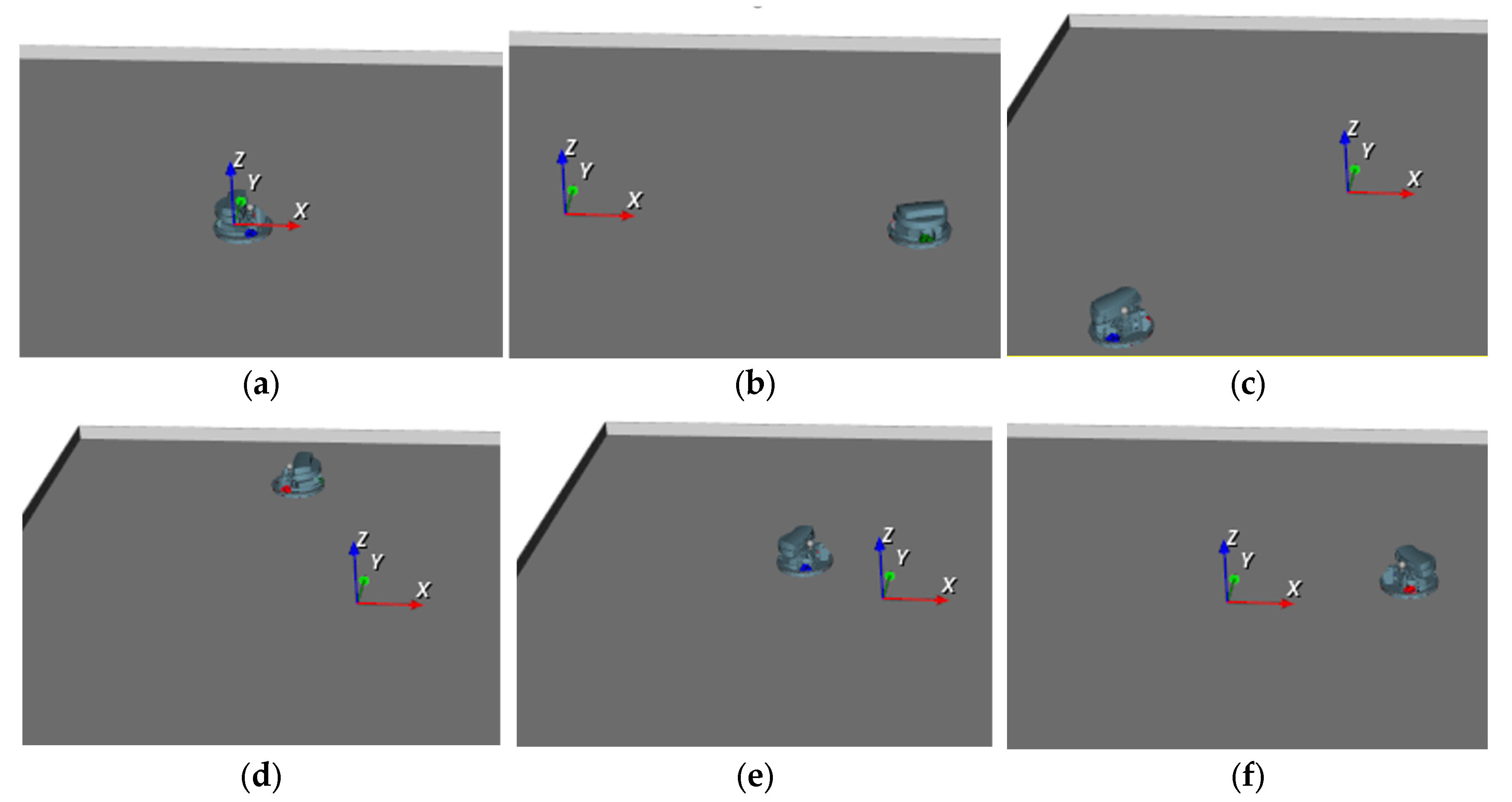
Virtual model of Robotino captured at different time instants during simulation is shown in Figure 27.
5. Conclusions
This paper proposes a novel methodology for 3D virtual modeling of the articulated mechanisms that can be driven by signals obtained from other model, for instance from its dynamic model developed using other software package.
Proposed approach uses well-known XML technology which provides systematically development of 3D visual model in form of a tree. But, instead editing of XML document, the operations are applied to the document tree in Tree View pane by inserting or removing the elements or attributes in environment of BondSim3DVisual. Simultaneously with DOM like tree a conventional XML code is also automatically generated and shown in a separate read-only pad.
The methodology explained in the paper has applied on modeling of the holonomic mobile robot (Robotino) equipped with three omnidirectional wheels. The 3D model of Robotino is created using 3D CAD models of robot parts in form of STL files. Virtually driving the articulated model by external signals is provided by developed dynamic model of robot using a separate general-purpose Bond Graph software BondSim. During the development of the dynamic model of the robot, the lateral rolling of the rollers of the robot’s omnidirectional wheels was also taken into account and described in the paper.
The two-way communication between two developed robot models—the dynamic and virtual is established. Both models run during simulation in different software packages and can communicate to each other. The dynamic model sends information to virtual one to drive it, but there is also communication in opposite direction. This means some information can be picked up from the virtual model and delivered to the dynamic (or any other). Thus, some information which can be more easily obtained on the virtual model, can be delivered from virtual to the dynamic side. To verify presented methodology a geometric rose with three petals used as an example of the plane curve that the center of the Robotino should follow.
In future research, it would be interesting to develop a more complex visual model of the environment in which the robot moves and to establish communication between the dynamic, virtual and real, physical robot—the Robotino, equipped with a complex sensor system to optimize its motion.
[1] It is a convention. The
real direction depends on design of drivers’ chains. It will be discussed later
when dealing with the wheels’ drivers.
[2] Operators “?:” are known as the question operators and represents
the inline version of if-then-else construct.
Author Contributions
Conceptualization, V.D. and M.C.H.; state of art and methodology, V.D. and M.C.H.; software, V.D.; validation, V.D. and M.C.H.; formal analysis, V.D. and M.C.H.; investigation, M.C.H.; model developments, V.D. and M.C.H.; data curation, V.D. and M.C.H.; writing—original draft preparation, V.D. and M.C.H.; review and editing, V.D. and M.C.H.; visualization, V.D. and M.C.H.; supervision, V.D. and M.C.H. Both authors have read and agreed to the published version of the manuscript.
Funding
This research was funded by Ministry of Science, Higher education and Youth, Canton Sarajevo.
Data Availability Statement
The data obtained by simulations in this study are available from the corresponding author, up-on reasonable request.
Conflicts of Interest
The authors declare no conflict of interest.
References
- Nusser, G.; Bühler, D.; Gruhler, G.; Küchlin, W. Reality-Driven Visualization of Automation Systems via The Internet Based On Java And XML. IFAC Proceedings Volumes 2001, 34, 497–502. [Google Scholar] [CrossRef]
- https://gazebosim.org/home (last accessed on 02.11.2024).
- Kim, S.; Peavy, M.; Huang, P.-C.; Kim, K. Development of BIM-Integrated Construction Robot Task Planning and Simulation System. Automation in Construction 2021, 127, 103720. [Google Scholar] [CrossRef]
- https://www. 11. 2024.
- Rajendran, G.; V, U.; O’Brien, B. Unified Robot Task and Motion Planning with Extended Planner Using ROS Simulator. Journal of King Saud University—Computer and Information Sciences, 1319. [Google Scholar] [CrossRef]
- http://wiki. 11. 2024.
- https://cyberbotics.com/ Webots: robot simulator (cyberbotics.com) (last accessed on 02.11.2024).
- Gu, X.; Zhang, A.; Yuan, L.; Xia, Y. Design and Dynamics Simulation of a Triphibious Robot in Webots Environment. In Proceedings of the 2021 IEEE International Conference on Mechatronics and Automation (ICMA); IEEE: Takamatsu, Japan, August 8, 2021; pp. 1268–1273. [Google Scholar]
- https://morse-simulator.github.io/ (last accessed on 02.11.2024).
- https://www.coppeliarobotics.com/ (last accessed on 02.11.2024).
- Bogaerts, B.; Sels, S.; Vanlanduit, S.; Penne, R. Connecting the CoppeliaSim Robotics Simulator to Virtual Reality. SoftwareX 2020, 11, 100426. [Google Scholar] [CrossRef]
- https://carla. 11. 2024.
- https://raisim.com/ (last accessed on 02.11.2024).
- Casini, M.; Garulli, A. MARS: A Matlab Simulator for Mobile Robotics Experiments. IFAC-PapersOnLine 2016, 49, 69–74. [Google Scholar] [CrossRef]
- http://carmen.sourceforge.net/intro.html (last accessed on 02.11.2024).
- https://moveit.ros.org/ (last accessed on 02.11.2024).
- Santos Pessoa de Melo, M.; Gomes da Silva Neto, J.; Jorge Lima da Silva, P.; Natario Teixeira, J.M.X.; Teichrieb, V. Analysis and Comparison of Robotics 3D Simulators. In Proceedings of the 2019 21st Symposium on Virtual and Augmented Reality (SVR); IEEE: Rio de Janeiro, Brazil, October, 2019; pp. 242–251. [Google Scholar]
- Coronado, E.; Mastrogiovanni, F.; Indurkhya, B.; Venture, G. Visual Programming Environments for End-User Development of Intelligent and Social Robots, a Systematic Review. Journal of Computer Languages 2020, 58, 100970. [Google Scholar] [CrossRef]
- Collins, J.; Chand, S.; Vanderkop, A.; Howard, D. A Review of Physics Simulators for Robotic Applications. IEEE Access 2021, 9, 51416–51431. [Google Scholar] [CrossRef]
- Farley, A.; Wang, J.; Marshall, J.A. How to Pick a Mobile Robot Simulator: A Quantitative Comparison of CoppeliaSim, Gazebo, MORSE and Webots with a Focus on Accuracy of Motion. Simulation Modelling Practice and Theory 2022, 120, 102629. [Google Scholar] [CrossRef]
- Kaur, P.; Liu, Z.; Shi, W. Simulators for Mobile Social Robots: State-of-the-Art and Challenges. 2022. [Google Scholar] [CrossRef]
- Gammieri, L.; Schumann, M.; Pelliccia, L.; Di Gironimo, G.; Klimant, P. Coupling of a Redundant Manipulator with a Virtual Reality Environment to Enhance Human-Robot Cooperation. Procedia CIRP 2017, 62, 618–623. [Google Scholar] [CrossRef]
- Ibari, B.; Bouzgou, K.; Ayad, R.; Benchikh, L.; Ahemed-Foitih, Z.; Bennaoum, M. Augmented Reality Environment for the Trajectory Tracking of Mobile Robot. In Proceedings of the 020 1st International Conference on Communications, Control Systems and Signal Processing (CCSSP); IEEE: EL OUED, Algeria, May 2020; pp. 278–281. [Google Scholar]
- Wu, M.; Dai, S.-L.; Yang, C. Mixed Reality Enhanced User Interactive Path Planning for Omnidirectional Mobile Robot. Applied Sciences 2020, 10, 1135. [Google Scholar] [CrossRef]
- Corke, P. Robotics, Vision and Control: Fundamental Algorithms In MATLAB® Second, Completely Revised, Extended And Updated Edition; Springer Tracts in Advanced Robotics; 2nd ed. 2017.; Springer International Publishing: Imprint: Springer: Cham, 2017; ISBN 978-3-319-54413-7. [Google Scholar]
- XML Technology, http://www.w3.org/standards/xml/;/; 2014 last accessed on 02.11.2024).
- BondSimulation. Available online: https://www.bondsimulation.com/ (accessed on 02.11.2024).
- Robotino Manual, 544305_robotino_deen2.pdf, //www.festo-didactic.com/media/customers/1100.
- Klimenda, F.; Cizek, R.; Pisarik, M.; Sterba, J. Stopping the Mobile Robotic Vehicle at a Defined Distance from the Obstacle by Means of an Infrared Distance Sensor. Sensors 2021, 21, 5959. [Google Scholar] [CrossRef] [PubMed]
- Castillo, O.; Cortés-Antonio, P.; Melin, P.; Valdez, F. Type-2 Fuzzy Control for Line Following Using Line Detection Images. IFS 2020, 39, 6089–6097. [Google Scholar] [CrossRef]
- Tang, Q.; Eberhard, P. Cooperative Search by Combining Simulated and Real Robots in a Swarm under the View of Multibody System Dynamics. Advances in Mechanical Engineering 2013, 5, 284782. [Google Scholar] [CrossRef]
- Damic, V.; Cohodar, M.; Omerspahic, A. Dynamic Analysis of an Omni-Directional Mobile Robot. Journal of Trends in the Development of Machinery and Associated Technology 17.
- Hadji, N.; Rahmani, A. Observer for an Omnidirectional Mobile Robot. In Proceedings of the Proceedings of the 2010 Spring Simulation Multiconference on—SpringSim ’10; ACM Press: Orlando, Florida, 2010; p. 1. [Google Scholar]
- Damic, V.; Cohodar, M.; Muratovic, M. Dynamic Modelling of Mobile Robots Based on Its 3D CAD Model. In DAAAM Proceedings; Katalinic, B., Ed.; DAAAM International Vienna, 2017; Vol. 1, pp. 0144–0149 ISBN 978-3-902734-11-2.
- Muratovic, M. Modeling and simulation of mobile robot by Simulink, Faculty of Mechanical Engineering, University of Sarajevo, Master thesis, 2017.
- Mercorelli, P.; Voss, T.; Strassberger, D.; Sergiyenko, O.; Lindner, L. A Model Predictive Control in Robotino and Its Implementation Using ROS System. In Proceedings of the 2016 International Conference on Electrical Systems for Aircraft, Railway, Ship Propulsion and Road Vehicles & International Transportation Electrification Conference (ESARS-ITEC); IEEE: Toulouse, France, November, 2016; pp. 1–6. [Google Scholar]
- Hijikata, M.; Miyagusuku, R.; Ozaki, K. Wheel Arrangement of Four Omni Wheel Mobile Robot for Compactness. Applied Sciences 2022, 12, 5798. [Google Scholar] [CrossRef]
- Tagliavini, L.; Colucci, G.; Botta, A.; Cavallone, P.; Baglieri, L.; Quaglia, G. Wheeled Mobile Robots: State of the Art Overview and Kinematic Comparison Among Three Omnidirectional Locomotion Strategies. J Intell Robot Syst 2022, 106, 57. [Google Scholar] [CrossRef] [PubMed]
- Qian, J.; Zi, B.; Wang, D.; Ma, Y.; Zhang, D. The Design and Development of an Omni-Directional Mobile Robot Oriented to an Intelligent Manufacturing System. Sensors 2017, 17, 2073. [Google Scholar] [CrossRef] [PubMed]
- Rubies, E.; Palacín, J. Design and FDM/FFF Implementation of a Compact Omnidirectional Wheel for a Mobile Robot and Assessment of ABS and PLA Printing Materials. Robotics 2020, 9, 43. [Google Scholar] [CrossRef]
- Manzl, P.; Sereinig, M.; Gerstmayr, J. A Mecanum Wheel Model Based on Orthotropic Friction with Experimental Validation. Mechanism and Machine Theory 2024, 193, 105548. [Google Scholar] [CrossRef]
- Crenganiș, M.; Breaz, R.-E.; Racz, S.-G.; Gîrjob, C.-E.; Biriș, C.-M.; Maroșan, A.; Bârsan, A. Fuzzy Logic-Based Driving Decision for an Omnidirectional Mobile Robot Using a Simulink Dynamic Model. Applied Sciences 2024, 14, 3058. [Google Scholar] [CrossRef]
- Wang, D.; Gao, Y.; Wei, W.; Yu, Q.; Wei, Y.; Li, W.; Fan, Z. Sliding Mode Observer-Based Model Predictive Tracking Control for Mecanum-Wheeled Mobile Robot. ISA Transactions 2024, 151, 51–61. [Google Scholar] [CrossRef] [PubMed]
- Damic, V.; Montgomery, J. Mechatronics by Bond Graphs: An Object-Oriented Approach to Modelling and Simulation; 2nd ed. 2015.; Springer Berlin Heidelberg: Imprint: Springer: Berlin, Heidelberg, 2015; ISBN 978-3-662-49004-4. [Google Scholar]
- Damic, V.; Cohodar, M. Multibody System Modeling, Simulation, and 3D Visualization. In Bond Graphs for Modelling, Control and Fault Diagnosis of Engineering Systems; Borutzky, W., Ed.; Springer International Publishing: Cham, 2017; ISBN 978-3-319-47433-5. [Google Scholar]
- Schroeder, W.; Martin, K.; Lorensen, B. The Visualization Toolkit: An Object-Oriented Approach to 3D Graphics; Visualize Data in 3D—Medical, Engineering or Scientific, Build Your Own Applications with C++, Tcl, Java or Python, Includes Source Code for VTK (Supports Unix, Windows and Mac), Eds.; 4. ed.; Kitware, Inc: Clifton Park, NY, 2006; ISBN 978-1-930934-19-1. [Google Scholar]
- Hanwell, M.D.; Martin, K.M.; Chaudhary, A.; Avila, L.S. The Visualization Toolkit (VTK): Rewriting the Rendering Code for Modern Graphics Cards. SoftwareX 2015, 1–2, 9–12. [Google Scholar] [CrossRef]
- The VTK User Guide, Kitware, Inc. https://vtk.org/vtk-users-guide/ (last accessed on 02.11.2024).
- Robotino® View—Programming—Robotino®—Services—Festo Didactic (festo-didactic.com) (last accessed on 15.04.2022).
- Simulation—Robotino®—Services—Festo Didactic (festo-didactic.com) (last accessed on 15.04.2022).
- pugixml 1.11, https://pugixml.org (last accessed 15.11.2020).
- www. 10. 2020.
- www.drukermotoren.com for (GR42x25), (last accessed on 02.11.2024).
- https://en.wikipedia.org/w/index.php?title=Rose_(mathematics)&oldid=808546190 (last accessed on 02.11.2024).
- Brenan, K.E.; Campbell, S.L.; Petzold, L.R. Numerical Solution of Initial-Value Problems in Differential-Algebraic Equations; Classics in applied mathematics; Unabridged, corr. republ., New York, 1989.; SIAM: Philadelphia, Pa, 1996; ISBN 978-0-89871-353-4. [Google Scholar]
Figure 1.
The components of real scene.
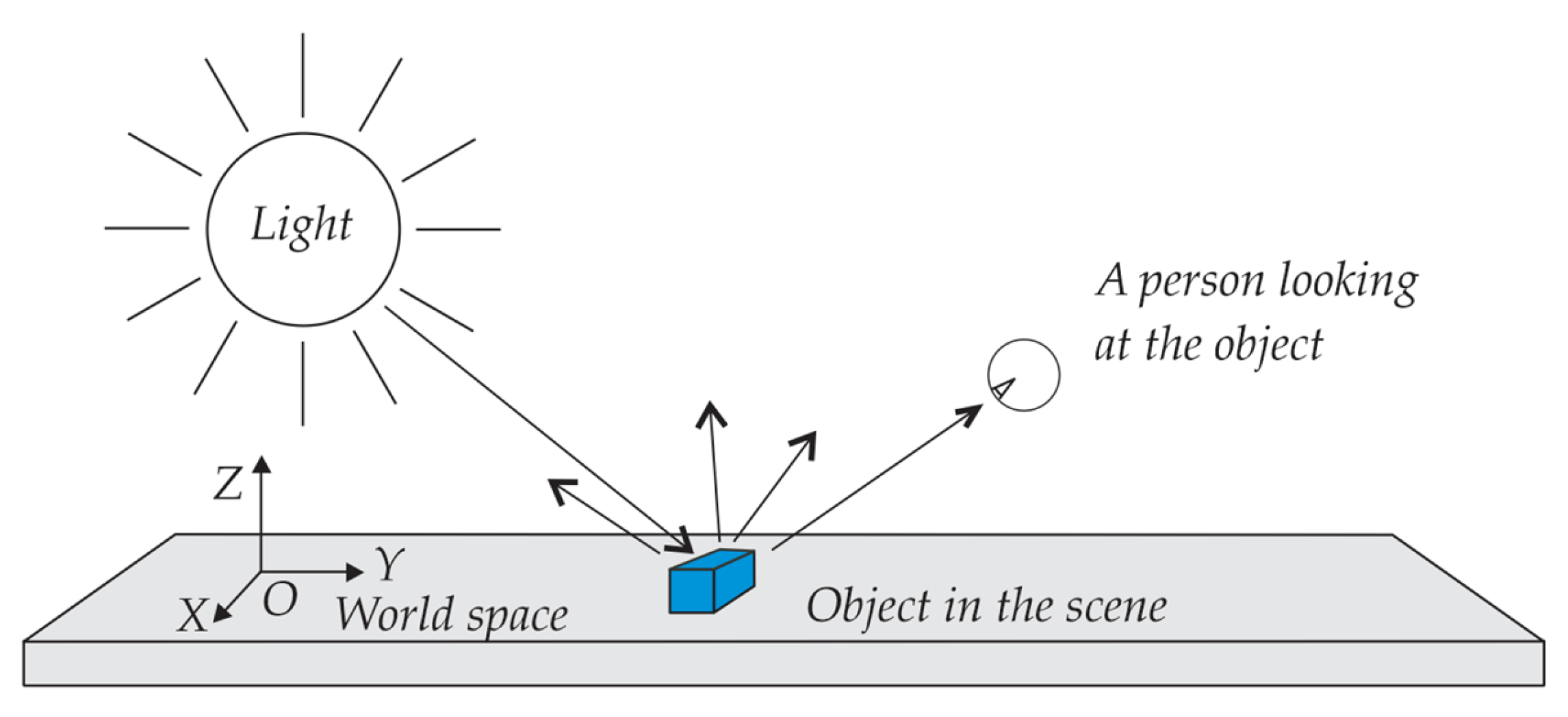
Figure 2.
The programming environment for visualization.
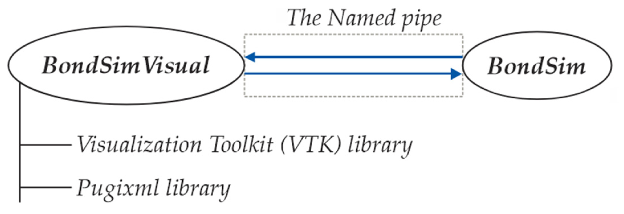
Figure 3.
BondSim3DVisual application’s mainframe.
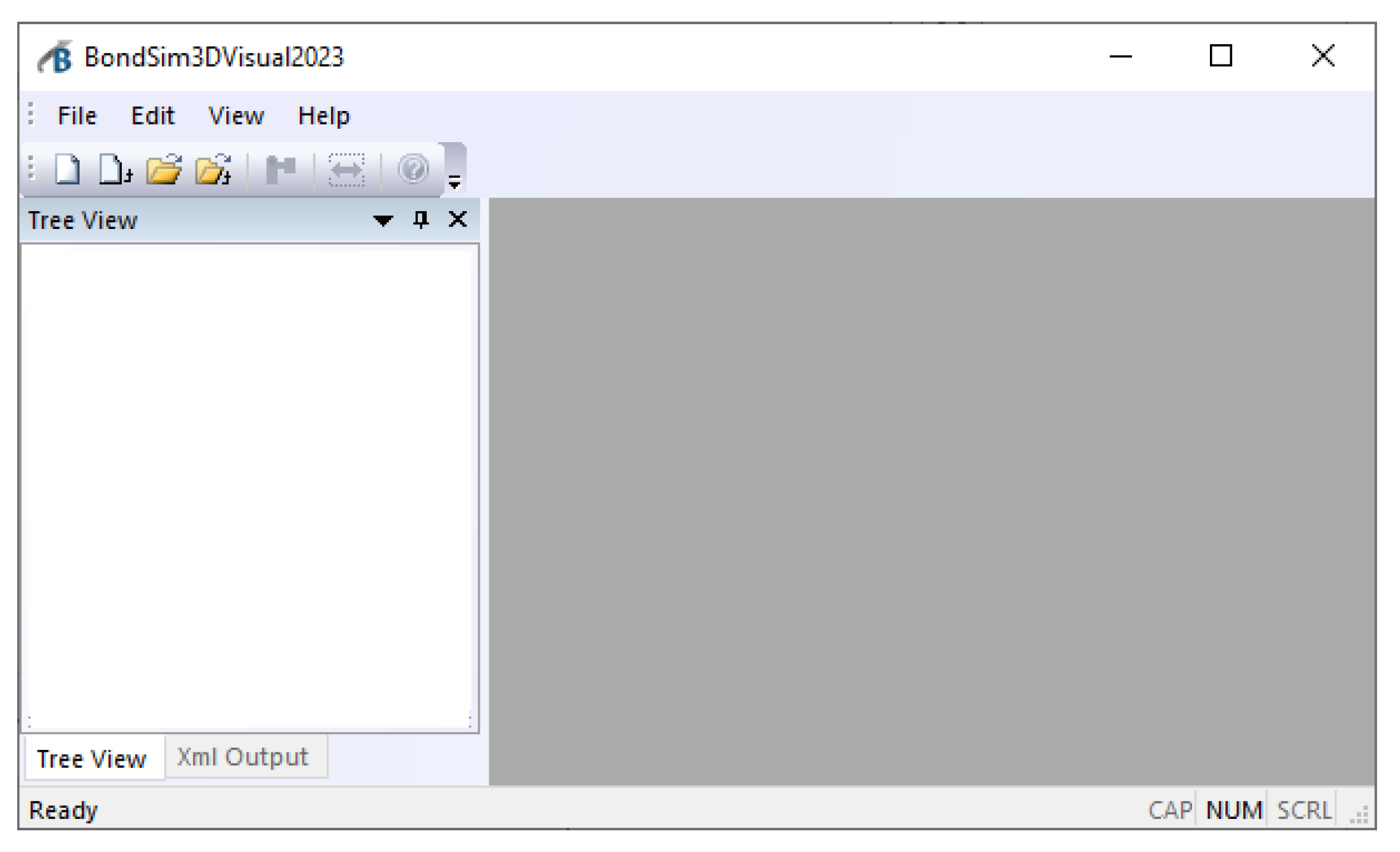
Figure 4.
Generated robot root: (a) Tree View; (b) XML Output.
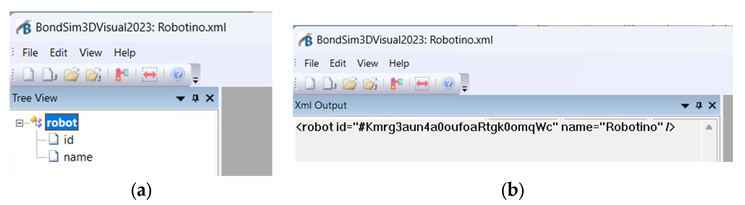
Figure 5.
(a) The menus for inserting an element or attribute; (b) Dialog window for selection the element which will be inserted into the tree.
Figure 5.
(a) The menus for inserting an element or attribute; (b) Dialog window for selection the element which will be inserted into the tree.

Figure 6.
(a) The coordinate frames associated with connected body links; (b) The XML segment describing the joint’s the next link transform.
Figure 6.
(a) The coordinate frames associated with connected body links; (b) The XML segment describing the joint’s the next link transform.
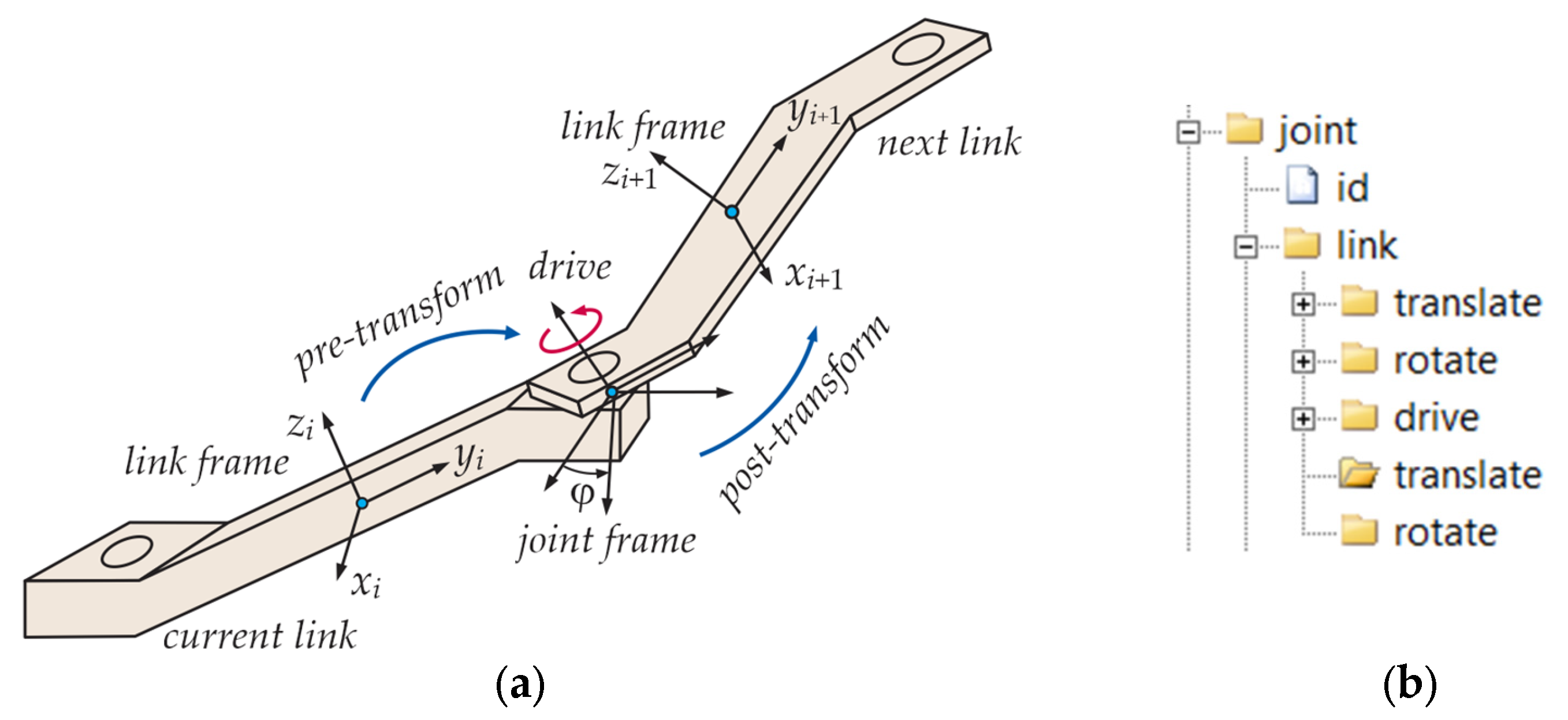
Figure 7.
Virtual model of: (a) Robotino; (b) its constitutive parts.
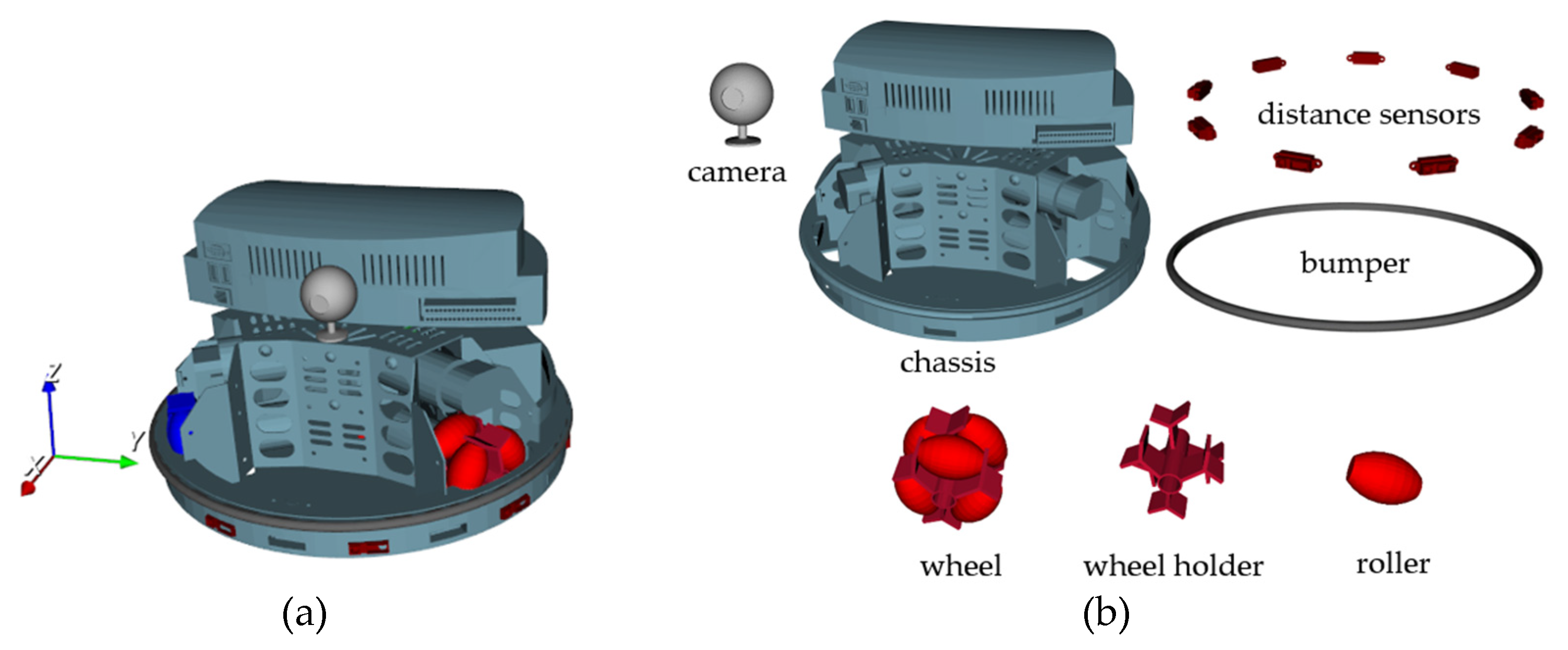
Figure 8.
Scheme of Robotino with world OXYZ and local Cxyz, Cixiyizi (i =1,2,3) coordinate frames.
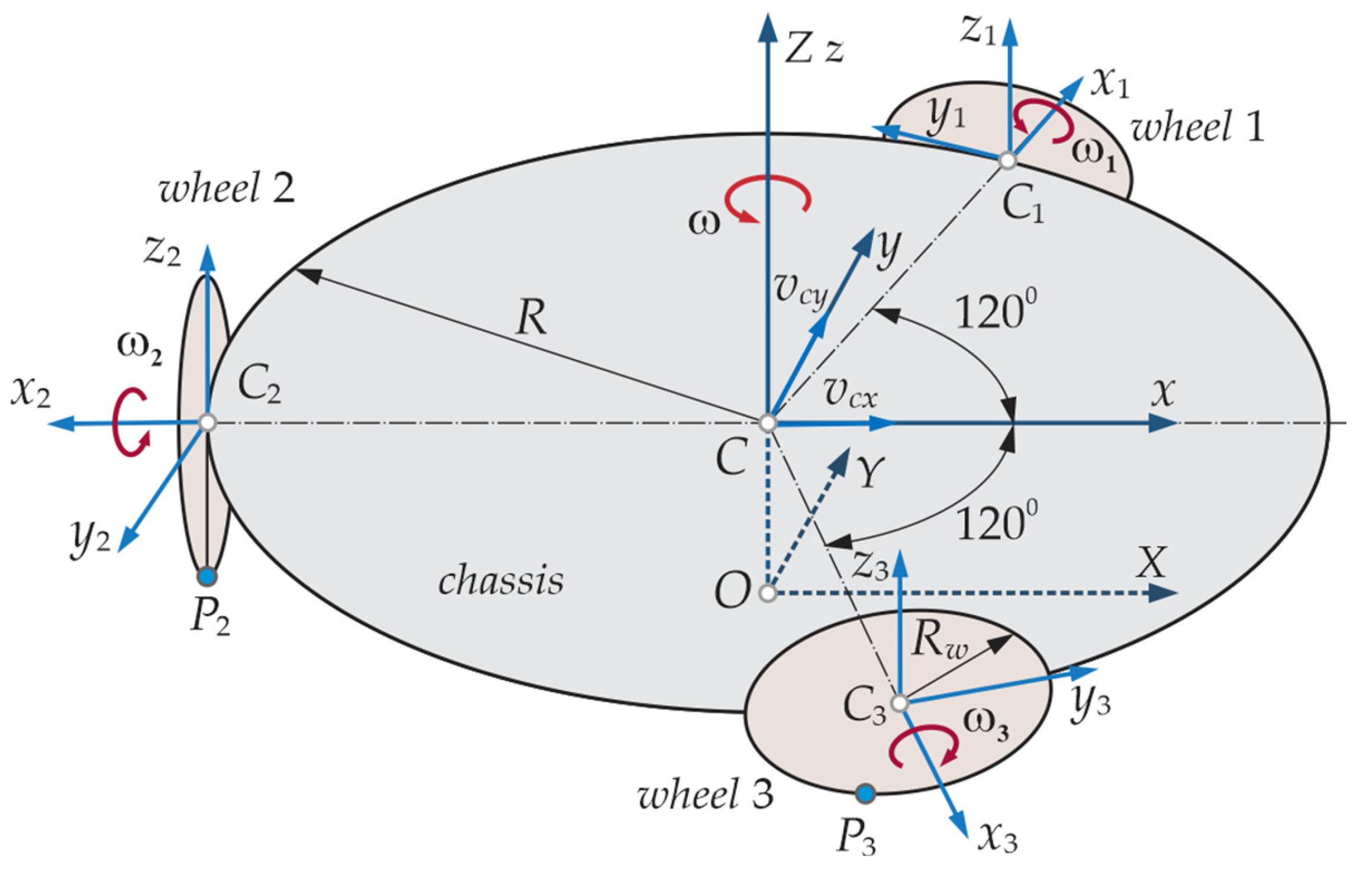
Figure 9.
The structure of the Robotino’s 3D model: (a) the basic; (b) of the wheels.
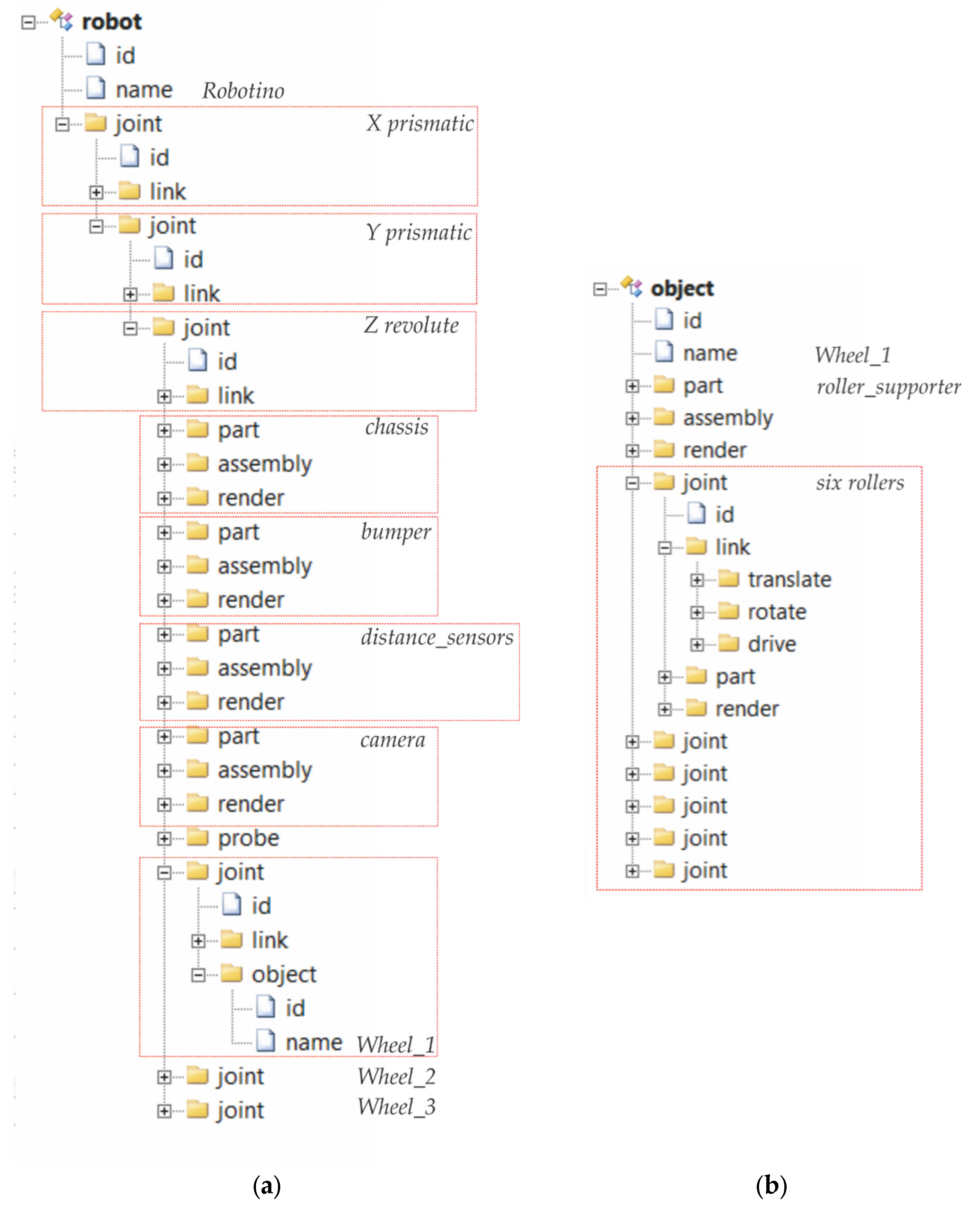
Figure 10.
The structure of: (a) Project Robotino; (b) Object’s Ground.
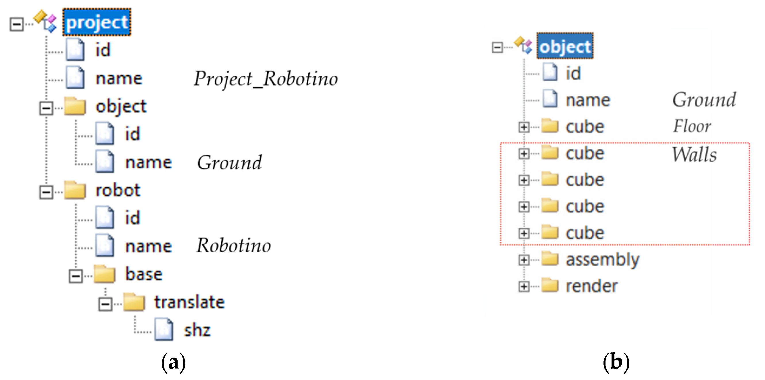
Figure 11.
Generated Robotino project view: (a) Normal; (b) Sized-up.
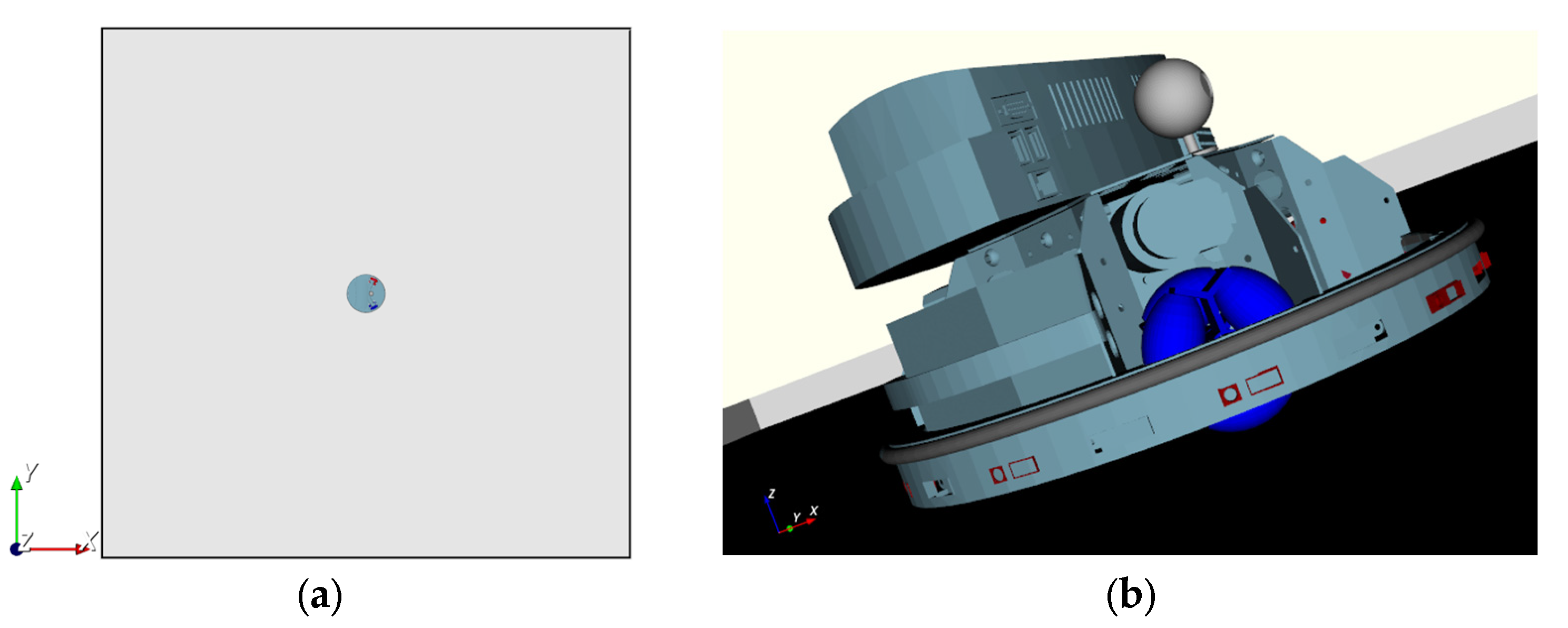
Figure 12.
Robotino’s base with the coordinate frames: Cxyz and Cixiyizi (i=1,2,3).
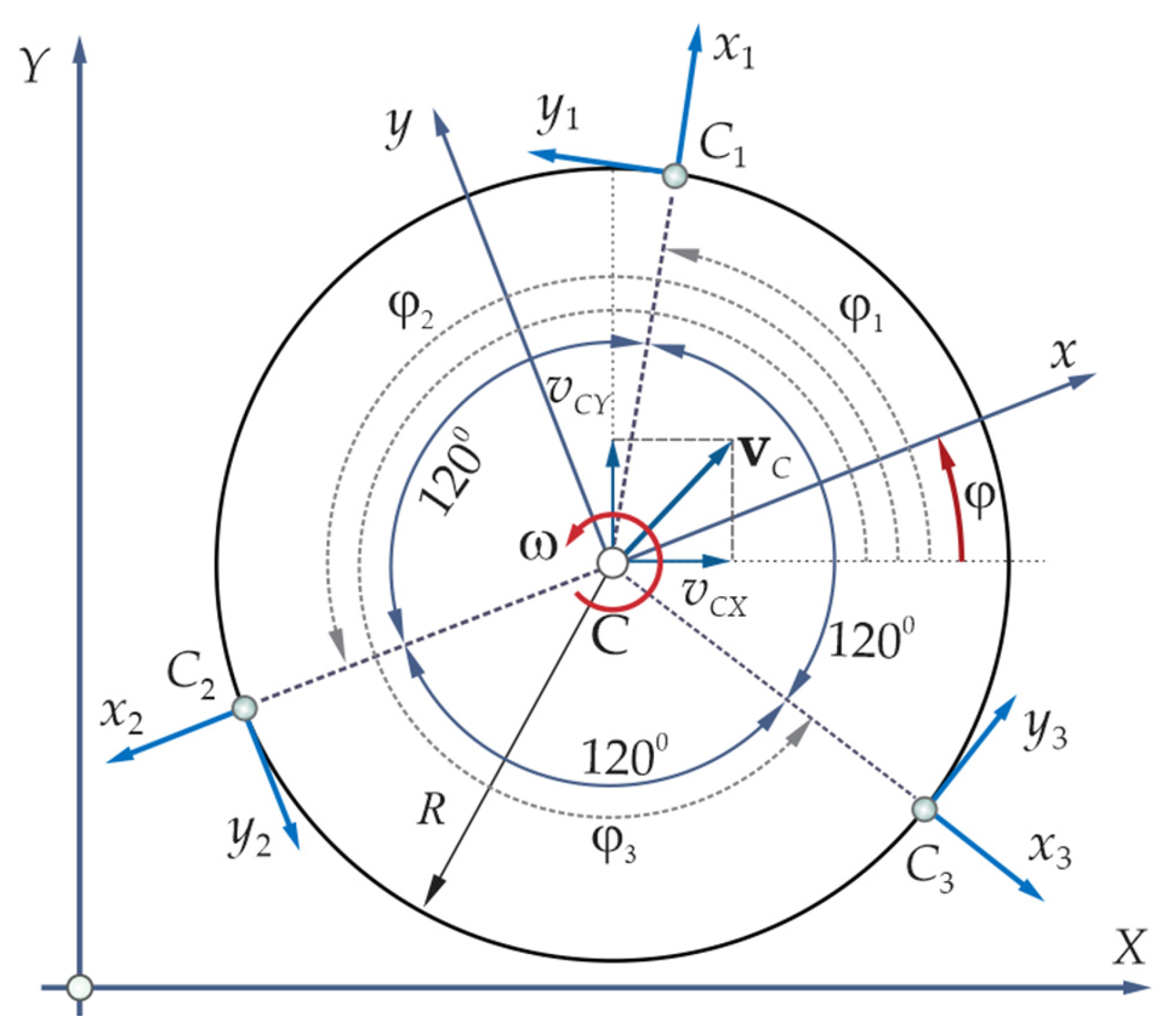
Figure 13.
Bond Graph representation of direct and invers coordinate transform: (a) The basic level; (b) Its structure.
Figure 13.
Bond Graph representation of direct and invers coordinate transform: (a) The basic level; (b) Its structure.
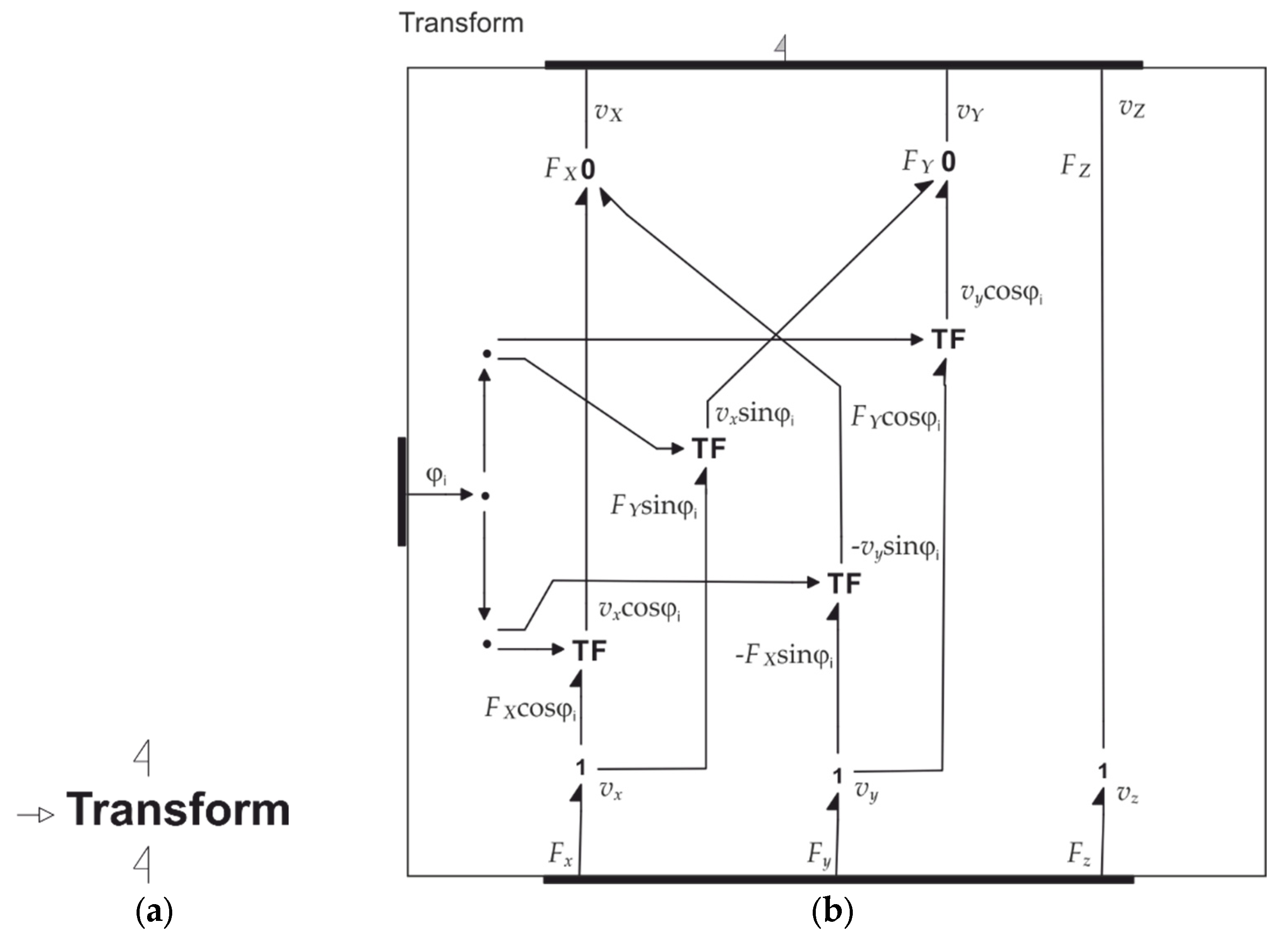
Figure 14.
The side view of a wheel.
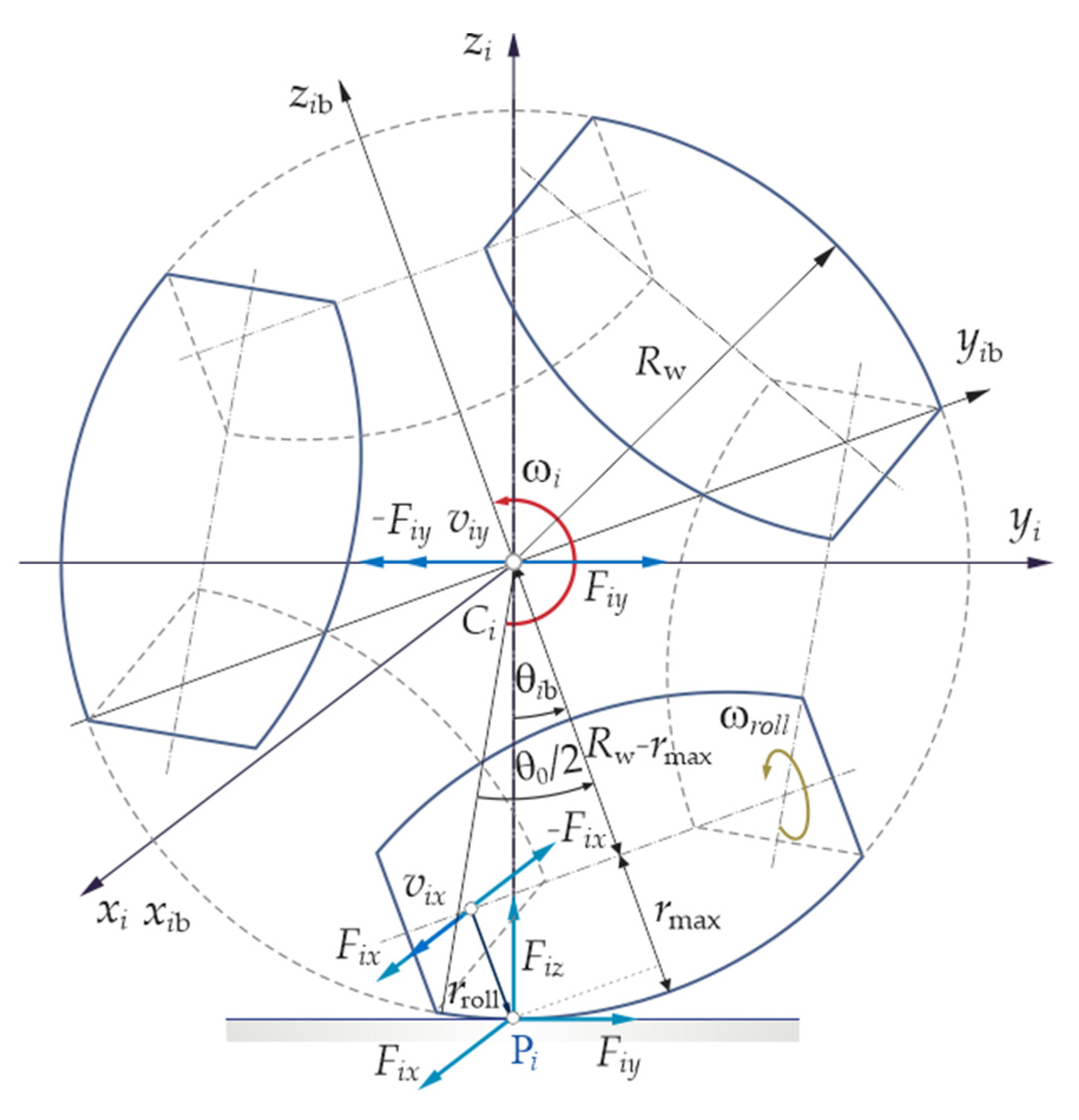
Figure 15.
Rotation to linear motion transform: (a) World model; (b) Its internal model.
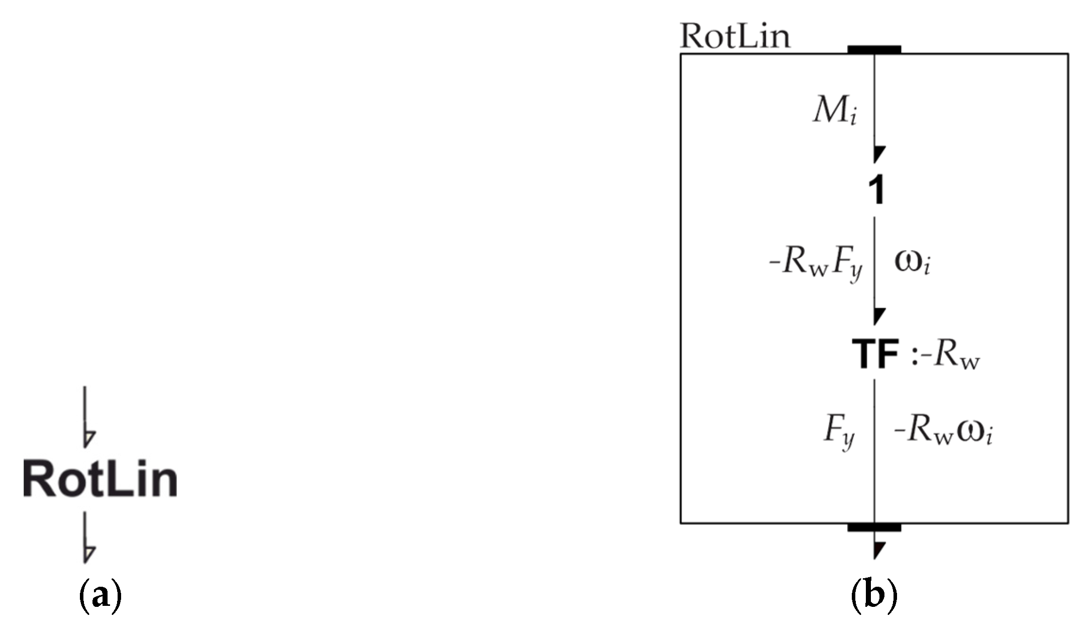
Figure 16.
Model of Roller: (a) The basic level; (b) Its structure; (c) Structure of LinRot.
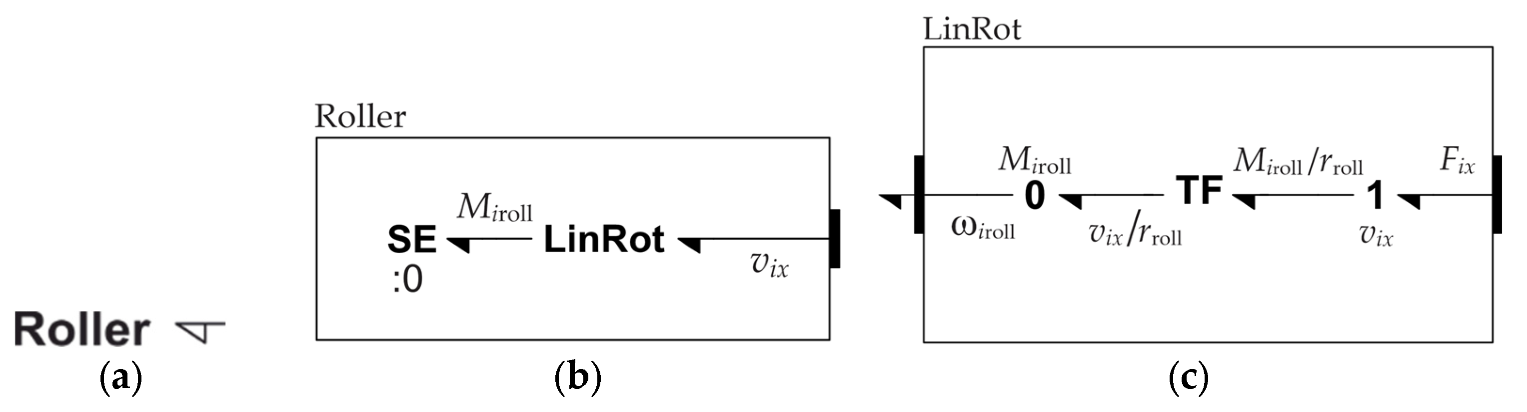
Figure 17.
(a) Rotation dynamic of the wheel; (b) Its internal model; (c) Transformation of variables; (d) Rotational dynamics.
Figure 17.
(a) Rotation dynamic of the wheel; (b) Its internal model; (c) Transformation of variables; (d) Rotational dynamics.
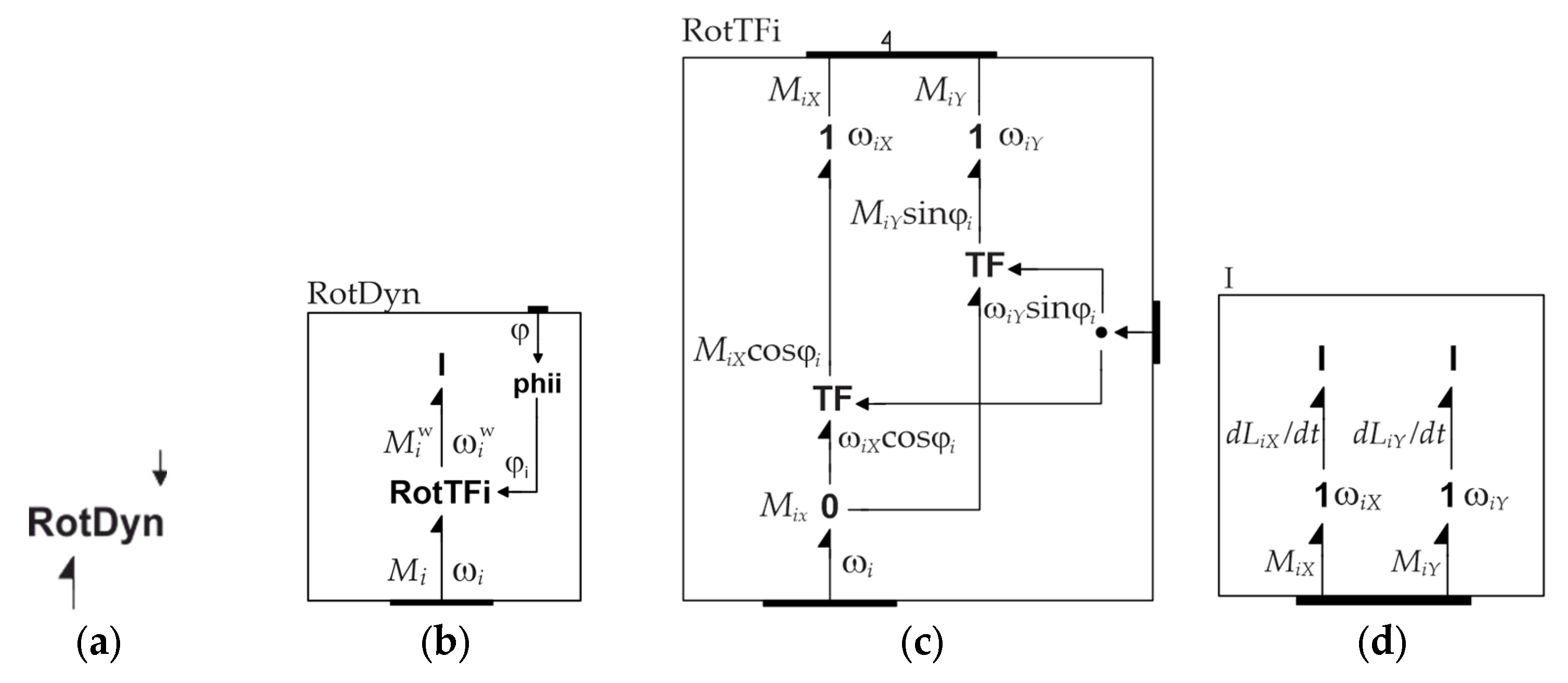
Figure 18.
The basic level Bond Graph model of the wheels.
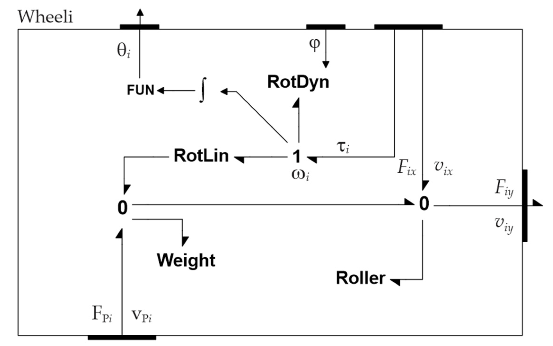
Figure 19.
Structure of Chassis model.
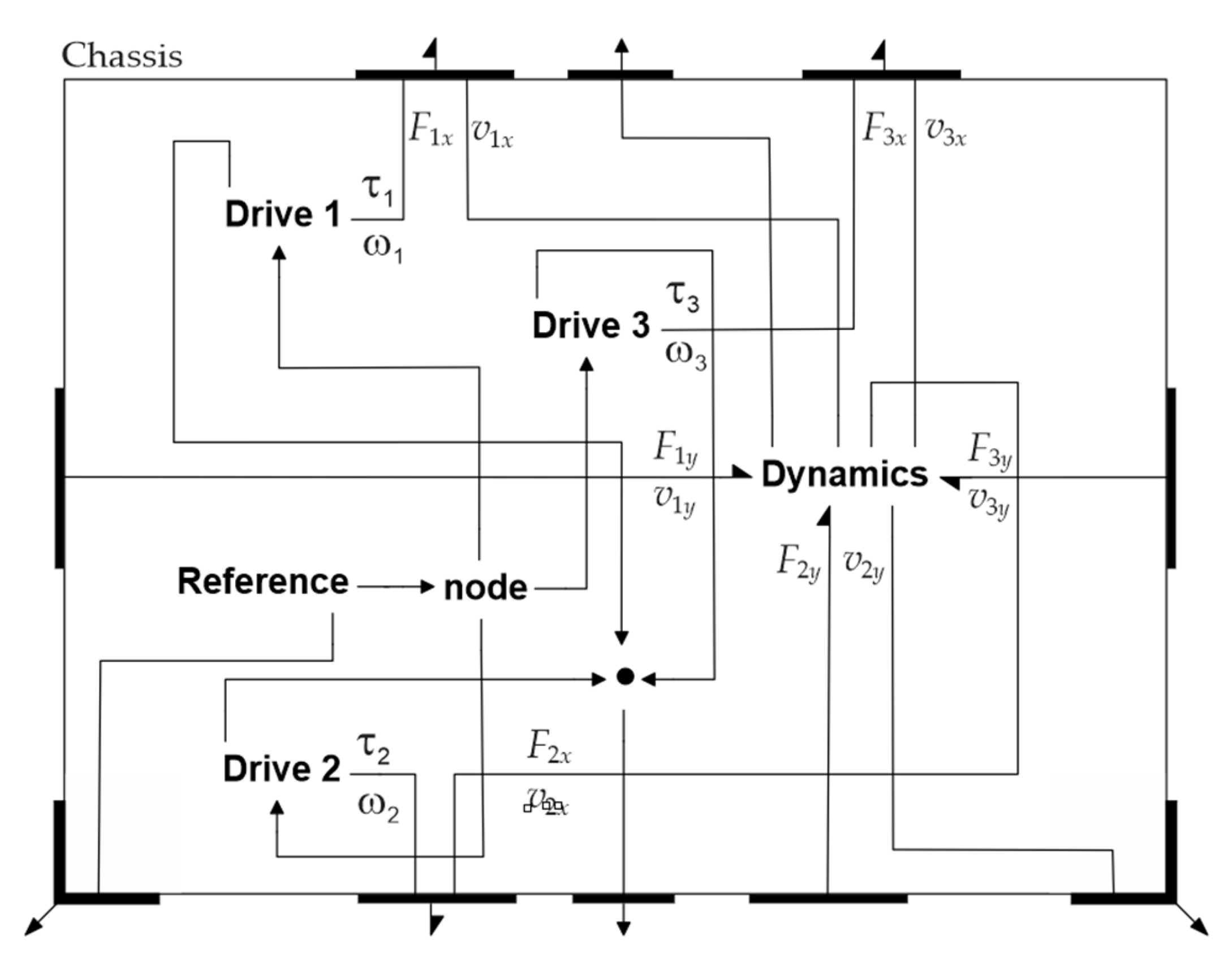
Figure 20.
Dynamics of the Chassis: (a) Structure of Dynamics model; (b) Structure of Transform.
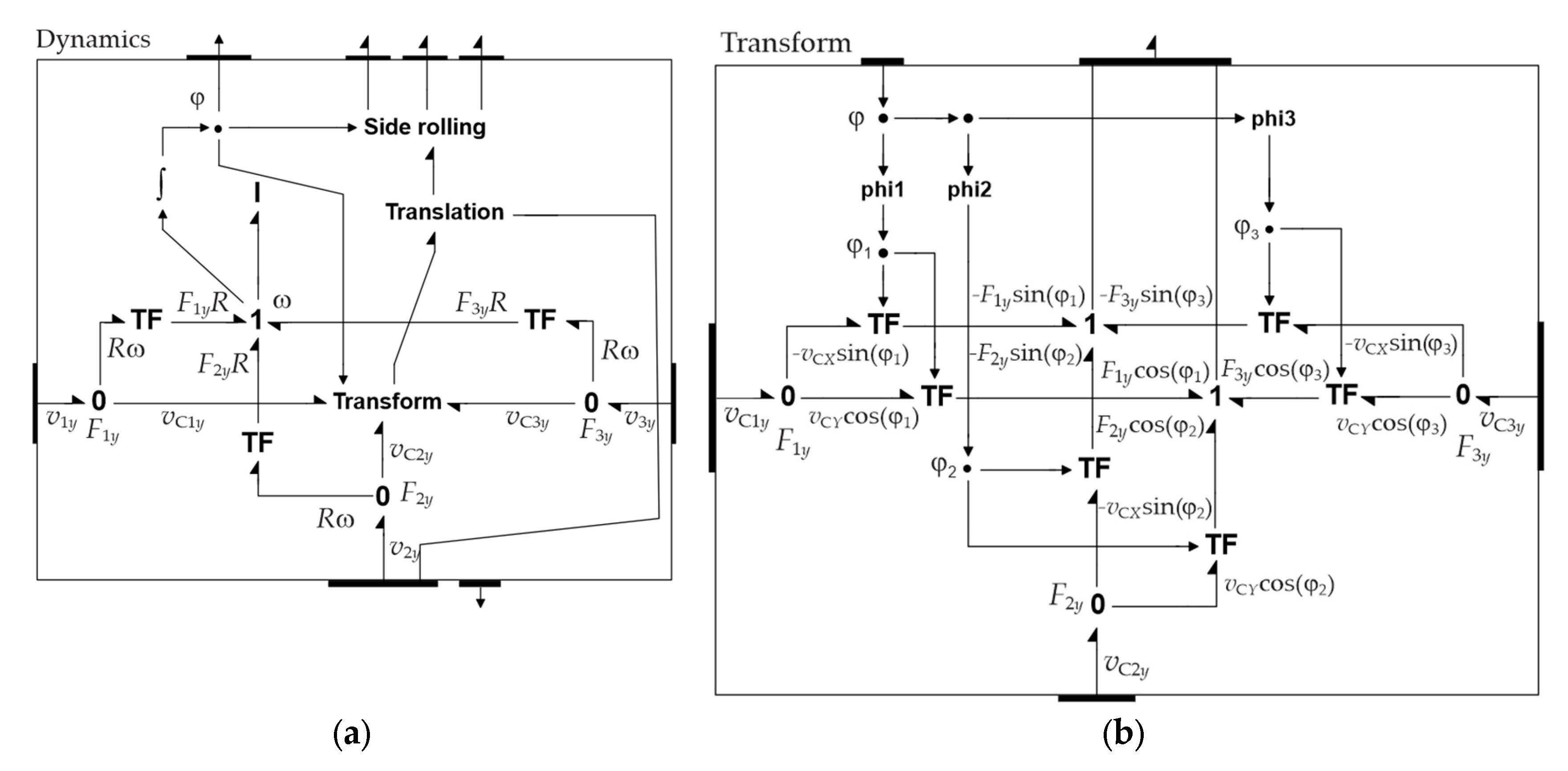
Figure 21.
(a) Structure of Side rolling; (b) Structure of Translation dynamics.
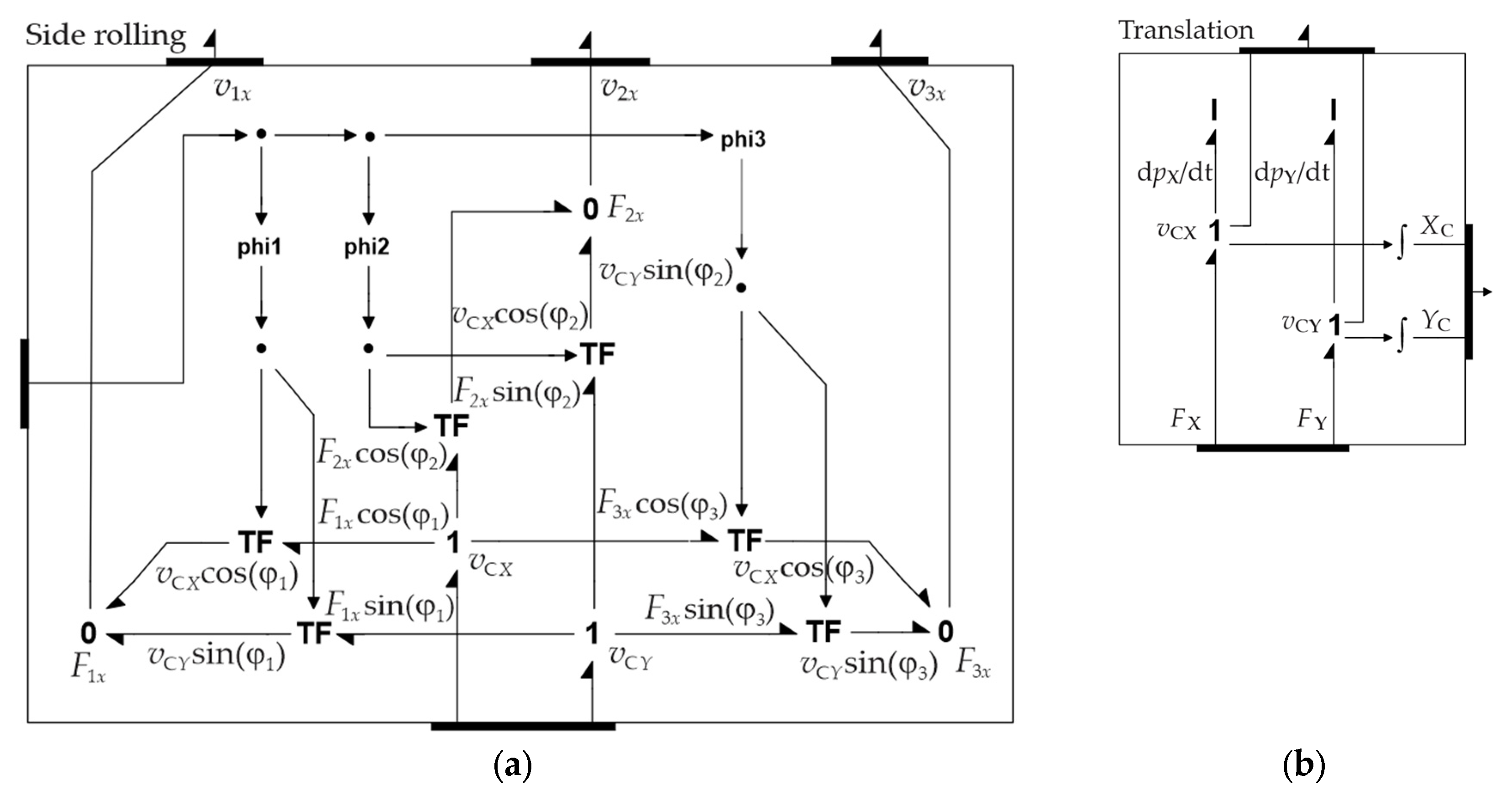
Figure 24.
Model of: (a) Ground; (b) vP1.
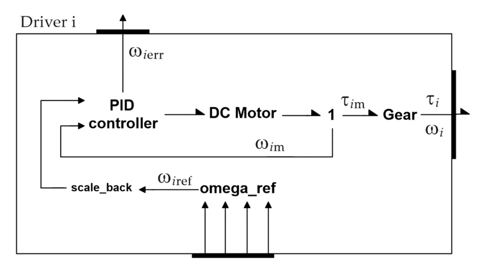
Figure 25.
The basic model of Robotino device.
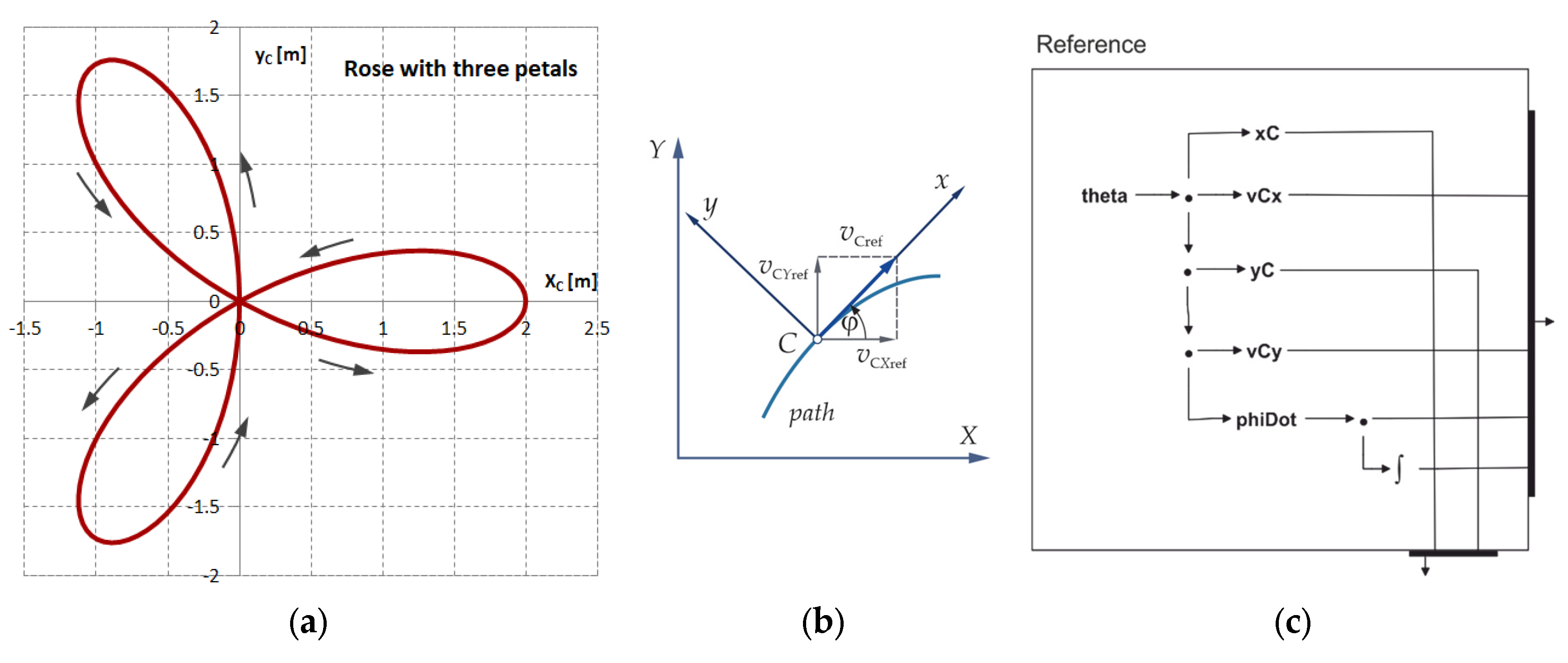
Figure 22.
Structure of the Driver 1 to Driver 3.
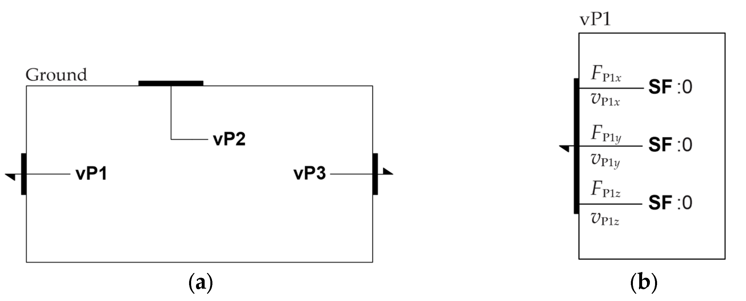
Figure 23.
Robotino path: (a) In the form of a rose; (b) The direction of the motion; (c) Reference functions.
Figure 23.
Robotino path: (a) In the form of a rose; (b) The direction of the motion; (c) Reference functions.
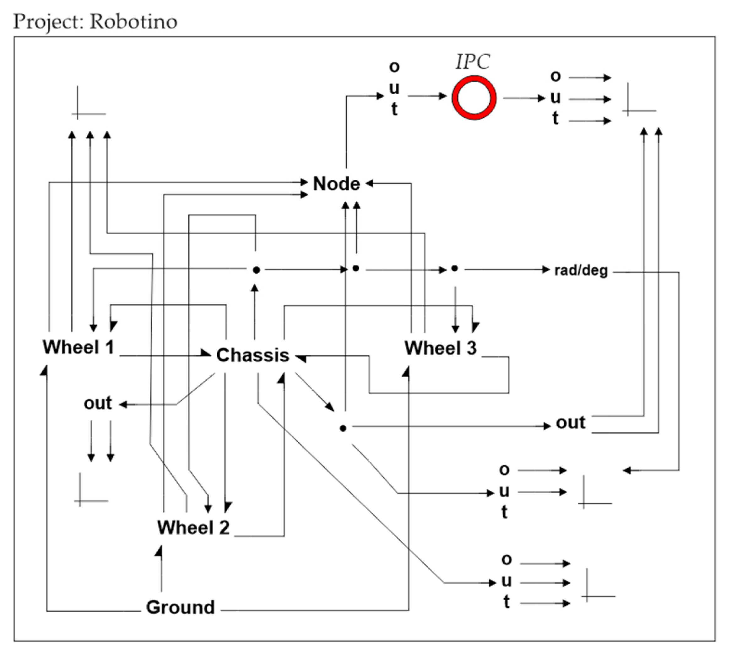
Figure 26.
Simulation results: (a) Path traversed; (b) Differences of XC and YC coordinates obtained with the virtual and dynamic models; (c) Differences of XC and YC coordinates obtained with dynamic model w.r.t. referent ones.
Figure 26.
Simulation results: (a) Path traversed; (b) Differences of XC and YC coordinates obtained with the virtual and dynamic models; (c) Differences of XC and YC coordinates obtained with dynamic model w.r.t. referent ones.
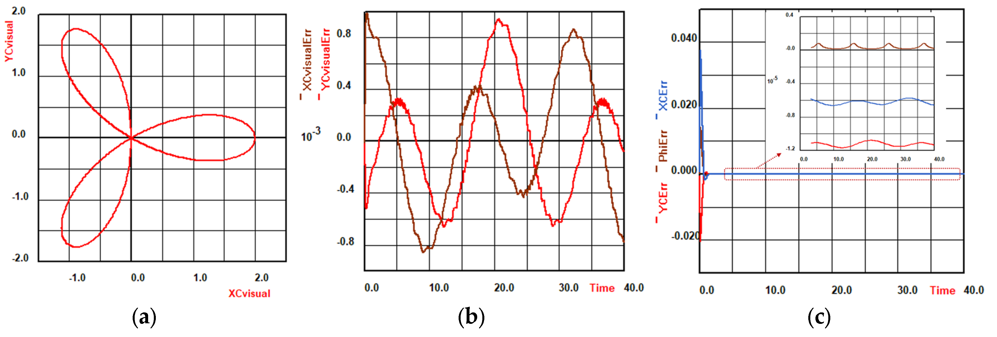
Figure 27.
The Robotino in motion: (a) t = 0 s; (b) t = 5 s; (c) t = 15 s; (d) t = 25 s; (e) t = 30 s; (f) t =40 s.
Figure 27.
The Robotino in motion: (a) t = 0 s; (b) t = 5 s; (c) t = 15 s; (d) t = 25 s; (e) t = 30 s; (f) t =40 s.
Disclaimer/Publisher’s Note: The statements, opinions and data contained in all publications are solely those of the individual author(s) and contributor(s) and not of MDPI and/or the editor(s). MDPI and/or the editor(s) disclaim responsibility for any injury to people or property resulting from any ideas, methods, instructions or products referred to in the content. |
© 2025 by the authors. Licensee MDPI, Basel, Switzerland. This article is an open access article distributed under the terms and conditions of the Creative Commons Attribution (CC BY) license (http://creativecommons.org/licenses/by/4.0/).
Copyright: This open access article is published under a Creative Commons CC BY 4.0 license, which permit the free download, distribution, and reuse, provided that the author and preprint are cited in any reuse.


