Submitted:
13 January 2025
Posted:
13 January 2025
You are already at the latest version
Abstract
Heart rate variability (HRV) which is the variation between consecutive heartbeats reflects the electrical activity of the heart and provides insight into autonomic nervous system (ANS) function. This study uses wavelet transform-based HRV feature extraction to investigate cardiac sympatho-vagal balance. Both Continuous Wavelet Transform (CWT) and Discrete Wavelet Transform (DWT) methods were applied in different steps. DWT was used for R-peak detection and CWT and MODWT were used to generate spectrograms from RR intervals. Frequency components (HF, LF, VLF) within 0.003-0.4Hz were extracted, and power estimation was performed. The LF/HF ratio, indicating sympatho-vagal balance, was calculated. ECG data from 42 arrhythmia patients and 18 normal sinus rhythm subjects were analyzed. The results showed a lower LF/HF ratio in arrhythmia patients, with higher HF power in arrhythmia subjects and higher LF power in normal sinus rhythm subjects. The study suggests that the parasympathetic nervous system dominates the ANS in arrhythmia patients, while the sympathetic nervous system dominates in normal sinus rhythm patients.
Keywords:
arrhythmia
; heart rate variability
; LF/HF ratio
; sympatho- vagal balance
; wavelet transform
1. Introduction
The human heart is crucial for sustaining life by pumping blood and delivering oxygen. Its rhythmic contractions, regulated by the autonomic nervous system (ANS), are influenced by the balance between the sympathetic nervous system (SNS) and the parasympathetic nervous system (PNS). This balance is called sympatho-vagal balance, significantly impacts heart rate variability (HRV), a key biomarker for cardiovascular [1]. HRV reflects fluctuations in the intervals between heartbeats and indicates the dynamic interaction between SNS and PNS. Healthy HRV shows good autonomic adaptability, while reduced HRV is linked to conditions like stress, cardiovascular diseases, and metabolic disorders [2].
Electrocardiography (ECG) records the electrical activity of the cardiac system as a signal [3] and provides data for HRV analysis. Traditional HRV analysis methods, such as time-domain and frequency-domain techniques, have limitations in localization and not suitable for non-stationary signals [4]. Wavelet transform analysis has emerged as a powerful tool for analyzing HRV and assessing cardiac sympatho-vagal balance with both time and frequency localized multi resolution analysis [5].
1.1. Wavelet Transformation
Wavelet theory was first proposed by the geophysicist Jean Morlet and the theoretical physicist Alex Grossmann in 1981. These wavelets are generated from a single function called “Mother Wavelet” which produces a family of functions by translation and dilation. The mother wavelet ψ (t) is given by the following equation. [6]
Where a is the scaling parameter and b is the translational parameter. The time widths of wavelets are adapted to their frequencies.
1.1.1. Wavelets
There are various wavelet families, including Morlet, Haar, Daubechies, Symlets, Gaussian, Mexican Hat, Mayer, and Biorthogonal wavelets. The wavelet chosen depends on the signal being processed. For ECG signal processing, Daubechies and Symlet wavelets are often used due to their similarity to ECG waveforms. The Daubechies family has 20 types (e.g., db2, db3, db4), and the Symlet family has 19 types (e.g., sym3, sym4, sym6). Figure 1. shows the db4 and sym4 wavelets used for ECG analysis.
1.1.2. Continuous Wavelet Transform (Cwt)
Continuous Wavelet Transform is the convolution of the signal x(t) with the scaled and translated version of the mother wavelet function Ψ(t). CWT is given by the following equation.
Where a is the scaling parameter and b is the translational parameter.
CWT is used in time-frequency analysis to process spectrograms and filtering purposes of time-localized frequency components.
1.1.3. Discrete Wavelet Transform (Dwt)
Discrete Wavelet Transform (Dwt) is the discretized scaled and translated version of the mother wavelet Ψ(t). DWT is given by the following equation.
In CWT, the integral is replaced with a summation as discrete values are considered. In DWT, the discrete values are represented as as and , where the dyadic power improves the efficiency of the analysis. DWT is used in multi-resolution analysis for tasks like signal denoising and signal compression [7,8]. Multiresolution Analysis
Wavelet analysis is a multi-resolution technique in both time and frequency domains, offering good localization in both. It provides better time resolution for higher frequencies and better frequency resolution for lower frequencies, as shown in Figure 2.(a) .High frequencies require good time resolution, achieved using narrow wavelets, while low frequencies spread over longer time durations, requiring wider wavelets for better frequency resolution [9]. Although multi-resolution analysis cannot simultaneously achieve perfect time and frequency resolution, it allows for optimal resolution in analyzing different frequency ranges.
1.1.4. Multilevel Decomposition
Multilevel decomposition is a technique for filtering high- and low-frequency components of a signal at multiple levels. At each level, the signal is split into detail coefficients (high-frequency) and approximation coefficients (low-frequency). The approximation coefficients capture the low-frequency components, while the detail coefficients capture the high-frequency components [10].
This is achieved by applying low-pass and high-pass filters (LPF and HPF) at each level. LPF captures lower frequencies while rejecting higher ones, and HPF captures higher frequencies while rejecting lower ones [11]. In Figure 2. (b), approximation and detail coefficients are represented by “A” and “D,” respectively. The approximation coefficients are iteratively filtered at each level in a dyadic process.
2. Materials and Methods
ECG data for HRV analysis were sourced from the trusted PhysioNet database [12], specifically the MIT-BIH Normal Sinus Rhythm and MIT-BIH Arrhythmia Databases. The Normal Sinus Rhythm Database includes 18 ECG recordings from patients referred to Beth Israel Deaconess Medical Center, have had not exhibit significant arrhythmias and involves 5 men aged from 26 to 45, and 13 women aged from 20 to 50. The recordings were sampled at a sampling rate of 128Hz.The Arrhythmia Database consists with 24-hour ambulatory ECG recordings of 47 patients, sampled at 360 Hz with 11-bit resolution [13].
The databases provide recordings in multiple formats (.atr, .dat, .hea, and .xws), which were challenging to handle. To ease processing, PhysioBank ATM offered ECG data in the more MATLAB-compatible .mat format. The process involved selecting the database and recording, setting the length to 1 hour, and exporting both .mat and .info files.
The .info file contains crucial data such as gain, base value, sampling frequency, and sampling time, which are needed for ECG waveform plotting.
Analysis was performed using MATLAB 2021a, selecting 18 recordings from the Normal Sinus Rhythm and 46 from the Arrhythmia database. The MLII channel (lead II) ECG signal was chosen for the Arrhythmia dataset, and the ECG1 signal for the Normal Sinus Rhythm dataset. Data from the .info files (sample rate, gain, and base values) were used in the analysis, with each step of the signal processing done using self-written code.
The ECG signal data was loaded into MATLAB using the command ecg=load('16265m.mat');, and the sampling rate, total number of samples, gain, and baseline were defined according to the .info file. Each ECG signal was normalized for consistency using the formula ecgsignal=((ecg.val)-base)/gain. A time vector was created corresponding to each sample point, and the ECG signal was plotted against this vector, comparing it with the waveform from PhysioBank ATM.
The next step involved locating the QRS complexes. Bandpass filtering was applied to identify R peaks within the QRS complexes, which contain middle frequencies in the ECG signal. For this, the maximal overlap discrete wavelet transform (MODWT) was used for wavelet decomposition. Different sampling frequencies in the normal sinus rhythm and arrhythmia datasets required different levels of decomposition. Previous studies have identified the QRS complex within the 0–50 Hz frequency range [14].
The MIT BIH normal sinus dataset, with a sampling frequency of 128Hz, was analyzed using the MODWT, computed down to 5 levels with the db4 wavelet. The corresponding frequency bands are shown in Table 1. The detail coefficients from levels 2, 3, 4, and 5 were retained, while the others were set to zero using the code:
wt = modwt(ecgsignal,5,'db4');
wtrec = zeros(size(wt));
wtrec(2:3:4:5,:) = wt(2:3:4:5,:);
Next, R peaks were isolated, and the inverse MODWT was applied to reconstruct the signal:
y = imodwt(wtrec,'db4');
To obtain positive peaks, the squared magnitude of the reconstructed signal was taken. R peaks were located using the findpeaks() function, with minimum peak distance and height determined by plotting the reconstructed signal. These values were applied to findpeaks() to identify the QRS peak position, time location, and isolated R peaks, which were then plotted (Figure 3.).
For the MIT BIH arrhythmia dataset, with a sampling frequency of 360Hz, the MODWT was computed down to 6 levels using the sym4 wavelet, providing the frequency bands shown in Table 2. Detail coefficients from levels 3, 4, 5, and 6 were retained, and the others were set to zero. The reconstructed signal was generated using IMODWT with the sym4 wavelet. The same R peak localization procedure as in the normal sinus dataset analysis was followed.
Additionally, MODWPT, another wavelet decomposition method, was used to locate R peaks, following the same steps as in the MODWT method. The final step was to calculate HRV using RR intervals.
HRV analysis, a key objective of this study, involves calculating the variation between consecutive heartbeats, or the distance between R peaks. This was done by using the code:
rr_intervals = diff(locs)*1000;
The difference between R peak time locations was used to compute the RR intervals. These values, initially in the millisecond range, were multiplied by 1000 to convert them into milliseconds. The RR interval values were then plotted against the beat number (Figure 4.), representing HRV.
Next, the frequency components of the RR intervals were extracted using CWT for time-frequency analysis. The sampling frequency and time vector of the RR intervals were calculated based on the number of RR intervals and the original ECG signal's sampling frequency:
rr_intervals_Fs = (length(rr_intervals)/length(samples))*Fs;
rr_intervals_t=(0:(length(rr_intervals)-1))/( rr_intervals_Fs*60);
The CWT spectrogram was then plotted using the cwt() function, as shown in Figure 5.
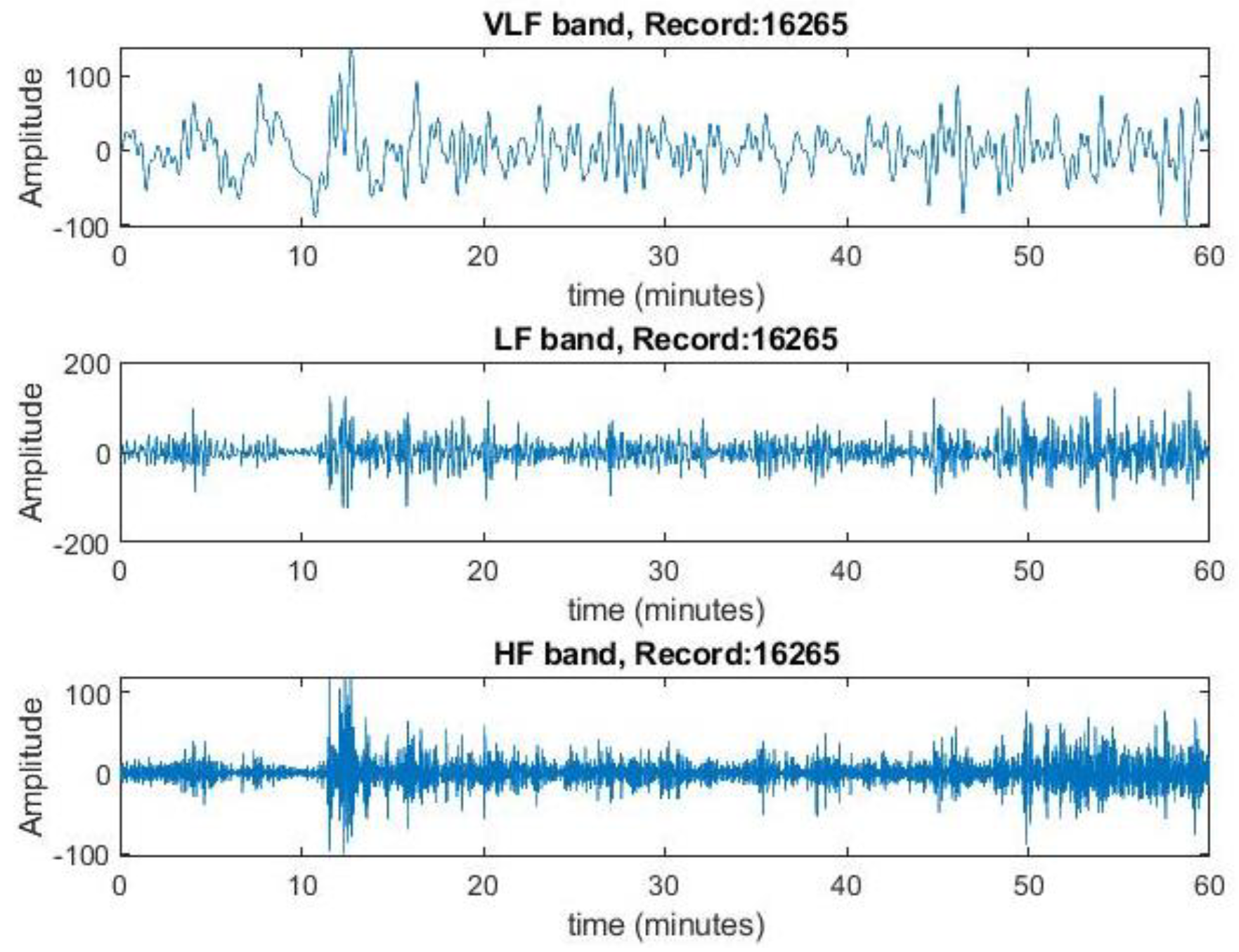
Inverse CWT was performed using the icwt( ) function to extract the time-localized VLF, LF, and HF components. This was done by reconstructing the signal for each frequency band separately. Here the frequency bands were taken as VLF range: 0.003 Hz - 0.04 Hz, LF range: 0.04 Hz - 0.15 Hz, and HF range - 0.15 Hz - 0.4 Hz for these long-term ECG signals [15]. These frequency components were then plotted separately against time.
Figure 6.
Extracted frequency components in VLF, LF and HF bands for record no.16265 from the spectrogram. This represents the variation of magnitude of rr intervals for each band.
Figure 6.
Extracted frequency components in VLF, LF and HF bands for record no.16265 from the spectrogram. This represents the variation of magnitude of rr intervals for each band.
The next step was to calculate the power of the VLF, LF, and HF bands. This was done by calculating the square of the root mean square (RMS) values of the reconstructed signals for each frequency band:
power_VLF = rms(vlf_reconstruct)^2;
The total power was then obtained by summing the powers of the VLF, LF, and HF bands. To facilitate comparison, the power values were normalized by dividing them by the total power. The LF/HF ratio was then computed by dividing the normalized power of the LF band by the normalized power of the HF band.
3. Results and Discussion
Electrocardiography (ECG) is a non-invasive method used to assess cardiac health by capturing the heart's electrical activity. Wavelet transformation is a promising technique for analyzing ECG signals, providing insights into heart rate variability (HRV).
This study analyzed HRV using wavelet transformation on 60 ECG recordings from the MIT-BIH Normal Sinus Rhythm and Arrhythmia databases. The analysis followed five main steps: locating R peaks, calculating RR intervals, generating spectrograms, extracting frequency bands, and determining the LF/HF ratio, using both Continuous Wavelet Transform (CWT) and Discrete Wavelet Transform (DWT).
Accurately locating R peaks is crucial, as the RR interval accuracy depends on it. Previous studies showed that MODWT and MODWPT methods were effective for R peak detection, with MODWPT offering better resolution. Thus, both methods were tested on six randomly selected recordings from both databases (Normal Sinus: 16265, 16786, 19140; Arrhythmia: 106, 112, 117) to evaluate their performance.
Except for recording no. 117, no significant differences were observed in R peak localization, RR intervals, and spectrogram plots generated using MODWPT and MODWT for these ECG recordings. This similarity is illustrated for recording no. 16786 in Figure 7 and Figure 8. The total power and LF/HF ratio of these recordings, computed using both MODWPT and MODWT methods, were nearly equal, except for recording no. 117, as shown in Table 3.
Figure 9 (a) and Figure 10 (a) show R peak localization for recording no. 117 using MODWPT and MODWT, respectively, revealing a significant difference in R peak localization from beat 0 to 600. The RR interval vs. beat number plot for MODWPT (Figure 9 (b)) also differs from the MODWT plot (Figure 10 (b)) until the 600th beat. While the spectrograms from both methods show no significant difference (Figure 9 (c) and Figure 10 (c)), the extracted frequency bands show a large difference in HF band power, confirming that MODWPT provides better resolution in the HF range than MODWT. This is because MODWPT decomposes both LF and HF components at each level, resulting in more filtered sub-frequency components, while MODWT only decomposes LF components. As a result, MODWPT offers better resolution in both LF and HF ranges, whereas MODWT performs better in LF components only.
However, the computational power required for MODWPT’s multilevel decomposition leads to longer processing times, and in some cases, the analysis failed due to memory issues. Therefore, the study continued with the MODWT method.
For the analysis, db4 and sym4 wavelets were used, as they resemble the QRS complex. The signals from the MIT-BIH normal sinus dataset were decomposed into 5 levels using db4, considering levels 2 to 5 for R peak localization. MIT-BIH arrhythmia signals were decomposed into 6 levels using sym4, with levels 3-6 considered. R peaks correspond to middle frequencies in the ECG signal, and previous studies suggest a sampling frequency around 50 Hz for QRS peaks, explaining the exclusion of higher frequency levels.
During the R peak localization process, missing R peaks were observed in normal sinus ECG recordings (no: 16420, 16483) and arrhythmia ECG recordings (no: 101, 111, 121, 201, 234). These missing peaks are highlighted in Figure 11. with a yellow circle.
The missing peaks in the analysis were likely caused by selecting inappropriate values for the “MinPeakDistance” and “MinPeakHeight” parameters in the “findpeaks” MATLAB function or by data loss during the initial R peak localization process. These missing peaks lead to erroneous higher RR intervals. When a peak is missing, the gap between the neighboring R peaks increases, resulting in an incorrectly calculated maximum interval. Figure 12 show RR interval plots for recordings no. 16420 and 121, highlighting the incorrect higher RR intervals due to these missing peaks.
Adjusting the minimum distance and height of the R peaks did not resolve the issue and instead led to more incorrect higher RR intervals in the RR interval plots. It is important to note that reducing these parameters too much also caused incorrect R peak identification. For example, in Figure 11. (b), many peaks with higher amplitudes than the missing R peaks were identified, leading to incorrect R peak inclusion. After successfully locating R peaks, RR intervals were calculated and plotted against the beat number. While some recordings showed incorrect higher intervals due to missing peaks, most recordings produced accurate RR interval plots. Figure 13. shows RR interval plots for recordings no. 16786 and 115, which resemble the reference plots from PhysioBank ATM.
For ECG recordings no. 16773 (Figure 14 (b)) and 18784, the reference RR interval plots from PhysioBank ATM displayed interruptions in the middle section, raising doubts about their accuracy. Consequently, these plots were considered incorrect.
Out of 60 recordings, only 7 showed inaccurate RR interval plots, so the study proceeded to the next steps of plotting spectrograms and extracting frequency components. CWT was applied to the RR interval signal to obtain spectrograms, where amplitude (energy) is represented by three dimensions: frequency increases along the y-axis, with lower-frequency components at the bottom. The cone of influence indicates more accurate data inside and less accurate data outside. The focus was on the HF, LF, and VLF components (0.003 Hz to 0.4 Hz). High-magnitude events were observed in some spectrograms, like for recordings 19093 and 228, but the study's main interest was analyzing HRV data through these frequency bands reflecting ANS activity.
Figure 15 (a) shows a spectrogram of a normal sinus rhythm ECG recording, where the LF and VLF ranges are brighter than the HF range, indicating higher LF power than HF power for this subject. This was consistent across all 18 normal sinus rhythm spectrograms. In contrast, Figure 15 (b) illustrates an arrhythmia ECG recording, where the HF range is brighter, indicating higher HF power than LF power. This pattern was observed in almost all 42 arrhythmia spectrograms. However, some arrhythmia recordings (e.g., 112, 123, and 222) also showed bright areas in the LF range, as shown in Figure 16.
Figure 16. show accurate RR interval plots, with higher variations in RR intervals due to the recordings themselves, not missing R peaks. These variations lead to high-magnitude events in the LF and HF regions, as seen in the spectrograms Figure 17. suggesting an unexpected LF/HF ratio. At the power estimation stage (Table 5), the LF/HF ratio for these recordings was higher than 1, deviating from other arrhythmia recordings.
Recording no. 16539, shown in Figure 18. (a), exhibited bright LF and VLF ranges typical of normal sinus rhythm, along with bright spots in the HF range after 35 minutes. The RR interval plot (Figure 18. (b)) shows that the variations are due to the recording, not missing R peaks. However, the power estimation (Table 4) indicated a lower LF/HF ratio than 1, deviating from other normal sinus recordings due to the higher magnitudes in the HF band.

Table 4.
Estimated Power values for MIT-BIH Normal sinus rhythm dataset.
| Record No. | Total Power | Normalized power (n.u) | LF/HF ratio | |||||
|---|---|---|---|---|---|---|---|---|
| VLF | LF | HF | VLF | LF | HF | |||
| 16265 | 982.206 | 797.42 | 251.961 | 2031.588 | 0.483 | 0.392 | 0.124 | 3.164 |
| 16272 | 3695.852 | 871.607 | 334.761 | 4902.22 | 0.753 | 0.177 | 0.068 | 2.603 |
| 16273 | 1923.648 | 613.323 | 213.616 | 2750.588 | 0.699 | 0.222 | 0.077 | 2.871 |
| 16420 | 497.22 | 634.57 | 56.026 | 1187.818 | 0.418 | 0.534 | 0.047 | 11.326 |
| 16483 | 505.501 | 648.268 | 81.5 | 1235.27 | 0.409 | 0.524 | 0.065 | 7.954 |
| 16539 | 2869.741 | 1244.762 | 2916.094 | 7010.597 | 0.409 | 0.174 | 0.415 | 0.42 |
| 16773 | 3323.282 | 2259.39 | 775.58 | 6358.26 | 0.522 | 0.355 | 0.121 | 2.913 |
| 16786 | 1284.794 | 1068.521 | 569.724 | 2923.039 | 0.439 | 0.365 | 0.194 | 1.875 |
| 16795 | 4178.642 | 1943.284 | 1074.122 | 7196.048 | 0.58 | 0.27 | 0.149 | 1.809 |
| 17052 | 3553.84 | 1132.412 | 6411.643 | 5327.416 | 0.667 | 0.212 | 0.12 | 1.766 |
| 17453 | 1568.02 | 1000.653 | 3384.886 | 2907.171 | 0.539 | 0.344 | 0.116 | 2.956 |
| 18177 | 1150.257 | 749.455 | 441.022 | 2340.735 | 0.491 | 0.320 | 0.188 | 1.699 |
| 18184 | 2325.916 | 1015.988 | 2211.593 | 3563.063 | 0.652 | 0.285 | 0.062 | 4.593 |
| 19088 | 727.481 | 366.368 | 231.762 | 1325.611 | 0.548 | 0.276 | 0.174 | 1.58 |
| 19090 | 1194.602 | 617.317 | 144.911 | 1956.831 | 0.61 | 0.315 | 0.074 | 4.259 |
| 19093 | 3770.705 | 1456.669 | 325.436 | 5552.81 | 0.679 | 0.262 | 0.058 | 4.476 |
| 19140 | 806.541 | 479.895 | 280.741 | 1567.178 | 0.514 | 0.306 | 0.179 | 1.709 |
| 19830 | 247.947 | 85.615 | 22.06 | 365.63 | 0.678 | 0.261 | 0.06 | 4.332 |
Table 5.
Estimated Power values for MIT-BIH Arrhythmia dataset.
| Index | Total Power | Normalized power (n.u) | LF/HF ratio | |||||
|---|---|---|---|---|---|---|---|---|
| VLF | LF | HF | VLF | LF | HF | |||
| 100 | 295.895 | 136.511 | 863.592 | 1295.999 | 0.228 | 0.105 | 0.666 | 0.158 |
| 101 | 740.593 | 508.507 | 967.957 | 2217.058 | 0.334 | 0.229 | 0.436 | 0.525 |
| 103 | 874.086 | 283.325 | 619.681 | 1777.093 | 0.491 | 0.159 | 0.348 | 0.457 |
| 105 | 278.359 | 291.088 | 1080.02 | 1649.463 | 0.168 | 0.176 | 0.654 | 0.269 |
| 106 | 4155.21 | 1863.38 | 18948.4 | 24967 | 0.166 | 0.074 | 0.758 | 0.098 |
| 107 | 83.027 | 275.126 | 904.511 | 1262.666 | 0.065 | 0.217 | 0.716 | 0.304 |
| 108 | 2258 | 3386 | 7143 | 12788 | 0.176 | 0.264 | 0.558 | 0.474 |
| 109 | 225.357 | 55.861 | 506.856 | 788.076 | 0.285 | 0.07 | 0.643 | 0.11 |
| 111 | 248.827 | 179.993 | 728.289 | 1157.111 | 0.215 | 0.155 | 0.629 | 0.247 |
| 112 | 108.338 | 37.878 | 36.819 | 183.036 | 0.591 | 0.206 | 0.201 | 1.02 |
| 113 | 2017.82 | 2532.15 | 4264.53 | 8814.49 | 0.228 | 0.287 | 0.483 | 0.593 |
| 114 | 836.476 | 788.307 | 5093.99 | 6718.77 | 0.125 | 0.117 | 0.758 | 0.154 |
| 115 | 3063.9 | 1841.02 | 1896.19 | 6801.099 | 0.45 | 0.27 | 0.278 | 0.97 |
| 116 | 267.311 | 574.905 | 1630.48 | 2472.701 | 0.108 | 0.232 | 0.659 | 0.352 |
| 117 | 1026.8 | 222.463 | 261.004 | 1510.326 | 0.679 | 0.147 | 0.172 | 0.852 |
| 118 | 898.244 | 699.618 | 1809.2 | 3407.059 | 0.263 | 0.205 | 0.531 | 0.386 |
| 119 | 966.203 | 1168.92 | 21469.9 | 23605 | 0.04 | 0.049 | 0.909 | 0.054 |
| 121 | 847.944 | 171.545 | 205.958 | 1225.449 | 0.691 | 0.139 | 0.168 | 0.832 |
| 122 | 928.243 | 128.752 | 71.893 | 1128.889 | 0.822 | 0.114 | 0.063 | 1.79 |
| 123 | 4304.29 | 6332.78 | 2945.29 | 13582.36 | 0.316 | 0.466 | 0.216 | 2.15 |
| 124 | 1353.45 | 435.352 | 1467.37 | 3256.174 | 0.415 | 0.133 | 0.45 | 0.296 |
| 200 | 691.461 | 881.709 | 3113.06 | 4686.227 | 0.147 | 0.188 | 0.664 | 0.283 |
| 201 | 22255 | 13128.3 | 31395.5 | 66778.85 | 0.333 | 0.196 | 0.47 | 0.418 |
| 202 | 4171.18 | 3406.07 | 8072.44 | 15649.7 | 0.266 | 0.217 | 0.515 | 0.421 |
| 205 | 128.279 | 81.507 | 378.745 | 588.532 | 0.217 | 0.138 | 0.643 | 0.215 |
| 209 | 2886.21 | 580.797 | 769.583 | 4236.593 | 0.681 | 0.137 | 0.181 | 0.754 |
| 210 | 1139.49 | 2012.61 | 4775.11 | 7927.211 | 0.143 | 0.253 | 0.602 | 0.421 |
| 212 | 345.922 | 380.276 | 539.868 | 1266.067 | 0.273 | 0.3 | 0.426 | 0.704 |
| 213 | 15.81 | 53.506 | 173.516 | 243.834 | 0.068 | 0.219 | 0.711 | 0.308 |
| 214 | 2396.8 | 3278.84 | 9936.07 | 15611.7 | 0.153 | 0.21 | 0.636 | 0.329 |
| 215 | 80.294 | 229.978 | 924.845 | 1235.119 | 0.065 | 0.186 | 0.748 | 0.248 |
| 217 | 661.746 | 749.83 | 2301.01 | 3712.586 | 0.178 | 0.201 | 0.619 | 0.325 |
| 220 | 1865.91 | 1179.83 | 3409.84 | 6455.575 | 0.289 | 0.182 | 0.528 | 0.346 |
| 221 | 1636.79 | 4791.15 | 15135.5 | 21563.49 | 0.075 | 0.222 | 0.701 | 0.316 |
| 222 | 6280.23 | 12581.8 | 8126.31 | 26988.38 | 0.232 | 0.466 | 0.301 | 1.54 |
| 223 | 649.899 | 333.746 | 971.99 | 1955.637 | 0.332 | 0.17 | 0.497 | 0.343 |
| 228 | 1758.14 | 2596.81 | 8272.69 | 12627.64 | 0.139 | 0.205 | 0.655 | 0.313 |
| 230 | 1894.66 | 991.77 | 308.061 | 3194.425 | 0.593 | 0.31 | 0.096 | 3.21 |
| 231 | 33216.2 | 4396.81 | 3197.72 | 40810.67 | 0.813 | 0.107 | 0.078 | 1.38 |
| 232 | 14254.9 | 111483 | 221810 | 347547.8 | 0.041 | 0.32 | 0.638 | 0.502 |
| 233 | 122.723 | 1905.31 | 1998.67 | 23119.26 | 0.053 | 0.082 | 0.864 | 0.095 |
| 234 | 393.933 | 113.916 | 167.856 | 675.706 | 0.582 | 0.168 | 0.248 | 0.678 |
Missing R peaks, leading to incorrect higher RR intervals, can also be seen as high-magnitude events in spectrograms. For example, Figure 19. shows a high magnitude between 15-20 minutes in the HF range due to a missing R peak, causing the overall spectrogram to appear dimmer. This condition is observed in all six recordings with missing R peaks.
CWT spectrograms of some recordings, Such as Figure 20. (a), show high magnitudes throughout, while others, like Figure 20 (b), display reduced brightness. This variation is due to each person having a unique ECG pattern, influenced by the structure of their heart, causing differences in signal magnitude and intensity [16].
The next step involved extracting frequency bands (VLF, LF, and HF) using inverse CWT, with frequency ranges set as VLF (0.003 Hz - 0.04 Hz), LF (0.04 Hz - 0.15 Hz), and HF (0.15 Hz - 0.4 Hz) for long-term ECG recordings [15]. The power of these bands was calculated by taking the square of the RMS values of the reconstructed signals, and power values were normalized to compare their contribution to total power. The LF/HF ratio was computed to assess the sympatho-vagal balance of the ANS. Power estimates are summarized in Table 4 and Table 5.
While the LF and HF bands are the main focus for the LF/HF ratio, the VLF band also contributes significantly to total power. The LF band is believed to reflect both sympathetic and parasympathetic activity, while the HF band reflects parasympathetic activity [17,18,19], though some studies suggest the LF band represents sympathetic activity [20,21]. However the LF/HF ratio is considered an indicator of the sympatho-vagal balance of ANS activity [22,23,24].
The power estimates for the normal sinus rhythm dataset in Table 4 show that normalized HF power is lower than LF power in most recordings, suggesting better activity in the LF range, potentially leading to an LF/HF ratio greater than 1.
Recording no. 16539 shows an LF/HF ratio of 0.42, the lowest observed in Table 4. Unlike other recordings, this one has a higher normalized power for the HF band than the LF band, resulting in a lower LF/HF ratio. The RR interval plot of this recording exhibited significant variation in RR intervals, likely due to variations in the ECG recording itself. This suggests that high HRV could lead to a lower LF/HF ratio, and the subject might have an undiagnosed heart condition or arrhythmia, though no conclusion can be made.
For recordings no. 16420 and 16483, the LF/HF ratio was much higher than in other recordings due to missing R peaks, which caused incorrect higher RR intervals. The estimated normalized HF power was very low, while LF power was higher. The spectrograms showed high-magnitude events in the HF region that spread into the LF range, leading to a higher LF/HF ratio.
Estimated power values for the arrhythmia dataset are shown in Table 5. In most cases, normalized LF power is lower than normalized HF power, indicating better activity in the HF range compared to LF. Except for six recordings, most LF/HF ratios were lower than 1, and the ratios in the arrhythmia dataset were generally lower than those in the normal sinus dataset.
Recording no. 106, 119, and 233 have very low LF/HF ratios, with abnormally low LF power compared to HF power. In the RR interval calculation step, large variations were observed in these recordings, which also appear as high-magnitude events in the HF range in the spectrograms (Figure 21 and Figure 22.). These variations suggest that high HRV could lead to a lower LF/HF ratio.
For recordings no. 112, 122, 123, 222, 230, and 231, the LF/HF ratio was higher than 1, as seen in the spectrograms (Figure 17.). These recordings showed high-magnitude events in both LF and HF ranges, with LF events brighter than HF. These variations were reflected in the RR interval plots and confirmed during power estimation, where the LF/HF ratio was higher than 1, deviating from other recordings.
To compare the LF/HF ratios between the normal sinus rhythm and arrhythmia datasets, scatter plots were created (Figure 23.), illustrating the LF/HF ratios of both groups.
Figure 23(a) shows the distribution of LF/HF ratios for normal sinus rhythm recordings, where most ratios are above 1, except for recording no. 16539, which deviated due to variations in RR intervals. Recordings no. 16420 and 16483 showed higher ratios due to missing R peaks causing incorrect high variations.
Figure 23(b) displays the LF/HF ratios for arrhythmia recordings, with most ratios below 1, except for six recordings. Recordings no. 112 and 115 had a ratio close to 1, indicating balanced parasympathetic and sympathetic nervous system activity.
Anomalous recordings in both datasets were due to high variations in RR intervals. In the normal sinus rhythm dataset, recording no. 16539 showed a low LF/HF ratio, while in arrhythmia recordings, high LF range power contributed to a higher LF/HF ratio. The comparison between both datasets shows that arrhythmia subjects are more likely to have a lower LF/HF ratio, indicating a dominance of the parasympathetic nervous system (PNS), while normal sinus rhythm subjects show a higher ratio, indicating sympathetic nervous system (SNS) dominance.
As a future work wavelet transform could be used in HRV analysis of patients suffering from different kinds of diseases and it could be also used to study the effect of gender and age on HRV.
4. Conclusions
Heart rate variability (HRV) reflects cardiac activity and overall autonomic nervous system health. Proper HRV analysis aids in identifying diseases and managing heart conditions. Using ECG signals from the PhysioNet database, HRV analysis employed Continuous Wavelet Transform (CWT) and Discrete Wavelet Transform (DWT) methods.
R peaks localization was performed using DWT methods: MODWPT and MODWT. MODWPT outperformed MODWT due to superior signal decomposition but was not continued due to computational limitations. Seven out of 60 recordings had missing R peaks due to data loss during initial localization.
CWT was applied to RR interval signals to generate spectrograms, revealing patterns related to heart conditions In these spectrograms high magnitude events were spotted. In some spectrograms power of the HF range was dominant, this was commonly observed in Arrhythmia ECG recordings. In some other spectrograms power of the LF range was dominant, this was commonly observed in normal sinus rhythm ECG recordings. CWT spectrogram of some recordings exhibited high magnitudes all over the spectrogram while, some other recordings displayed a reduction in brightness throughout the spectrogram. The reason is every person has a unique pattern in ECG due to the different structures of their hearts and therefore the ECG signal can vary in magnitude having low or high intensities depending on the person.
Frequency band extraction using ICWT reconstructed HF, LF, and VLF bands (0.003–0.5 Hz). Power estimation, calculated as the square of RMS values of reconstructed signals, indicated significant differences in LF/HF ratios between normal sinus rhythm and arrhythmia datasets. Normal sinus rhythm often showed abnormally low LF/HF ratios due to dominant HF power, while arrhythmia datasets exhibited abnormally high LF/HF ratios due to dominant LF power.
Scatter plot analysis confirmed lower LF/HF ratios in arrhythmia datasets, indicating a parasympathetic dominance, whereas normal sinus rhythm datasets showed sympathetic dominance. This highlights the use of wavelet-based HRV analysis for distinguishing autonomic regulation patterns in cardiac health and disease.
References
- Berntson, G. G., Thomas Bigger, J., Eckberg, D. L., Grossman, P., Kaufmann, P. G., Malik, M., Nagaraja, H. N., Porges, S. W., Saul, J. P., Stone, P. H., & Van Der Molen, M. W. (1997). Heart rate variability: Origins methods, and interpretive caveats. Psychophysiology, vol. 34(6), pp. 623-648. [CrossRef]
- Kim, Hye-Geum, Cheon, Eun-Jin, Bai, Dai-Seg, Lee, Y. Hwan, Koo and Bon-Hoon.(2008). Stress and heart rate variability: a meta-analysis and review of the literature, Psychiatry investigation, vol. 15, p. 235,. [CrossRef]
- German-Sallo and Zoltan. (2014). Wavelet transform based HRV analysis, Procedia Technology, vol. 12, pp. 105--111. [CrossRef]
- Shaffer, Fred, Ginsberg and J. P.(2017). An overview of heart rate variability metrics and norms,Frontiers in public health, vol. Frontiers, p. 258. [CrossRef]
- Boashash and Boualem.(2015). Time-frequency signal analysis and processing: a comprehensive reference, Academic press.
- Daubechies and Ingrid, Ten lectures on wavelets, SIAM, 1992.
- Mallat, S.G. (1989) A Theory for Multiresolution Signal Decomposition: The Wavelet Representation. IEEE Transactions on Pattern Analysis and Machine Intelligence, 11, 674-693. [CrossRef]
- O. Rioul. (1993). A discrete-time multiresolution theory. IEEE Transactions on Signal Processing, 41, 8 (August 1993), 2591–2606. [CrossRef]
- Pale, Una, Th{\"u}rk, Florian, Kaniusas and Eugenijus. (2016), Heart rate variability analysis using different wavelet transformations. [CrossRef]
- Acharya, U. R., Vidya, K. S., Ghista, D. N., Lim and W. J., (2015).Computer-aided diagnosis of diabetic subjects by heart rate variability signals using discrete wavelet transform method, Knowledge-based systems, vol. 81, pp. 56--64. [CrossRef]
- Ergen and Burhan.(2013). Comparison of wavelet types and thresholding methods on wavelet based denoising of heart sounds, Journal of Signal and Information Processing, vol. 4, p. 164. [CrossRef]
- A. L. Goldberger, L. A. Amaral, L. Glass, J. M. Hausdorff, P. C. Ivanov, R. G. Mark, J. E. Mietus, G. B. Moody, C.-K. Peng and H. E. Stanley.(2000). PhysioBank, PhysioToolkit, and PhysioNet: components of a new research resource for complex physiologic signals, circulation. [CrossRef]
- Moody G.B., Mark R.G. The impact of the MIT-BIH arrhythmia database. IEEE Eng. Med. Biol. Mag. 2001;20:45–50. [CrossRef]
- M. Elgendi, M. Jonkman and F. De Boer. (2010).Frequency Bands Effects on QRS Detection, Biosignals. [CrossRef]
- Malik, M., Bigger, J. T., Camm, A. J., Kleiger, R. E., Malliani, A., Moss, A. J., & Schwartz, P. J. (1996). Heart rate variability: Standards of measurement, physiological interpretation, and clinical use. European Heart Journal, 17(3), 354–381. [CrossRef]
- M. N. Dar, M. U. Akram, A. Usman and S. A. Khan.(2015).ECG biometric identification for general population using multiresolution analysis of DWT based features, 2015 Second International Conference on Information Security and Cyber Forensics (InfoSec). [CrossRef]
- A. Hernando, H. Posada-Quintero, M. D. Peláez-Coca, E. Gil and K. H. Chon.(2022). Autonomic Nervous System characterization in hyperbaric environments considering respiratory component and non-linear analysis of Heart Rate Variability,Computer Methods and Programs in Biomedicine. [CrossRef]
- B. Pomeranz, R. Macaulay, M. A. Caudill, I. Kutz, D. Adam, D. Gordon, K. M. Kilborn, A. C. Barger, D. C. Shannon and R. J. Cohen.( 1985). Assessment of autonomic function in humans by heart rate spectral analysis, American Journal of Physiology-Heart and Circulatory Physiology. [CrossRef]
- M. L. Appel, R. D. Berger, J. P. Saul, J. M. Smith and R. J. Cohen.(1989).Beat to beat variability in cardiovascular variables: noise or music?, Journal of the American College of Cardiology. [CrossRef]
- A. Malliani, M. Pagani, F. Lombardi and S. Cerutti.(1991).Cardiovascular neural regulation explored in the frequency domain.," Circulation. [CrossRef]
- N. Montano.(1994).Power spectrum analysis of heart rate variability to assess the changes in sympathovagal balance during graded orthostatic tilt., Circulation. [CrossRef]
- U. P. S. T. Task Force, U. S. O. o. D. Prevention and H. Promotion, (1996).Guide to clinical preventive services: report of the US Preventive Services Task Force, S Department of Health and Human Services, Office of Public Health and~…. [CrossRef]
- J. Sztajzel.(2004). Heart rate variability: a noninvasive electrocardiographic method to measure the autonomic nervous system, Swiss medical weekly. [CrossRef]
- M. Pagani, F. Lombardi, S. Guzzetti, O. Rimoldi, R. Furlan, P. Pizzinelli, G. Sandrone, G. Malfatto, S. Dell'Orto and E. Piccaluga.(1986).Power spectral analysis of heart rate and arterial pressure variabilities as a marker of sympatho-vagal interaction in man and conscious dog.," Circulation research. [CrossRef]
Figure 1.
db4 and sym4 wavelets. The sym4 wavelet is from the Symlet family, db4 is from the Daubechies family. These wavelets show similarities with the ECG signal waveform and are used in analyzing the ECG signal waveforms.
Figure 1.
db4 and sym4 wavelets. The sym4 wavelet is from the Symlet family, db4 is from the Daubechies family. These wavelets show similarities with the ECG signal waveform and are used in analyzing the ECG signal waveforms.
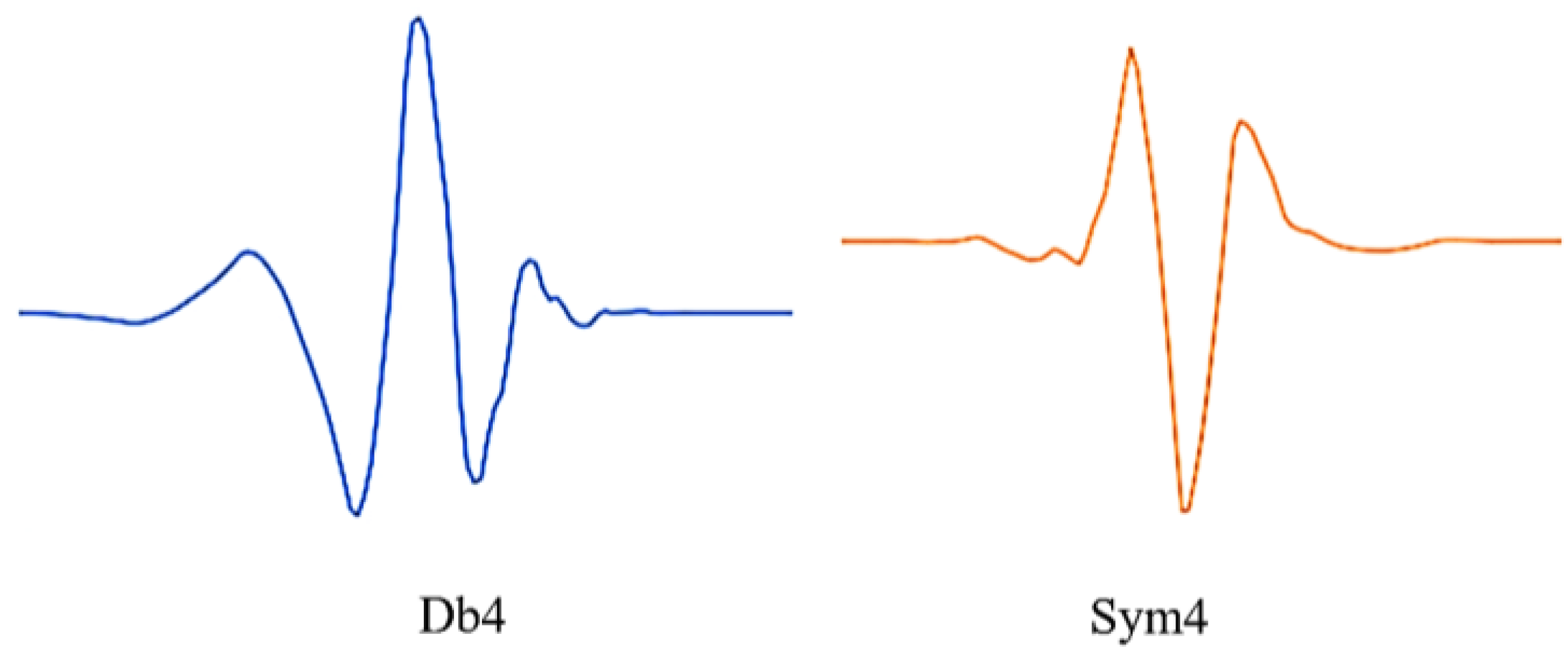
Figure 2.
(a) Graphical representation of multiresolution analysis. Wider wavelets (windows) are used in multi-resolution analysis to capture lower frequencies which provide high frequency resolution and narrow wavelets (windows) are used to capture higher frequencies which provide high time resolution. Figure 2. (b) Multi level decomposition. The approximation coefficients are shown by "A" and detailed coefficients are shown by "D". At each level the number of coefficients is halved.
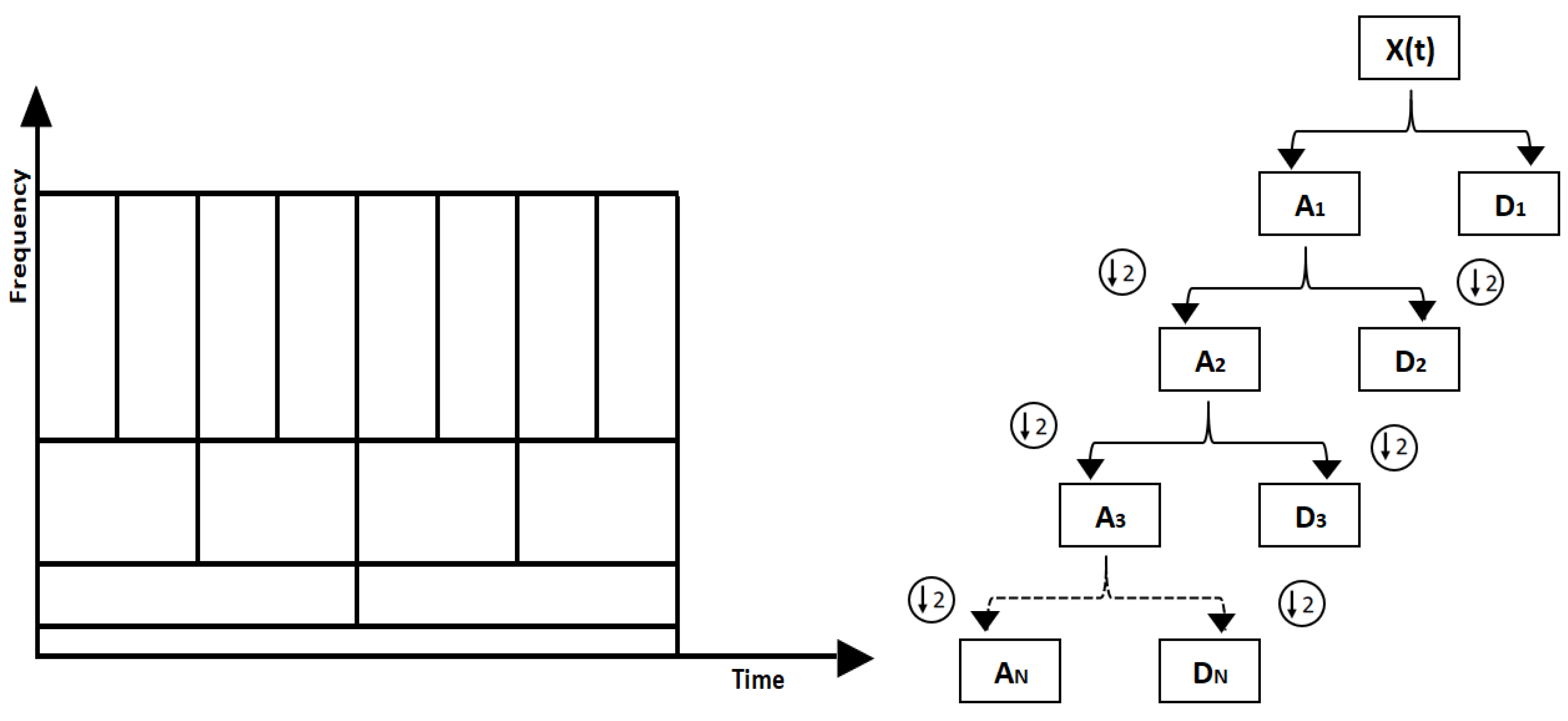
Figure 3.
ECG signal of normal sinus rhythm recording – 16265. Y axis represent the voltage amplitudes of the ECG signal and x axis represent the time duration of the ECG signal.
Figure 3.
ECG signal of normal sinus rhythm recording – 16265. Y axis represent the voltage amplitudes of the ECG signal and x axis represent the time duration of the ECG signal.
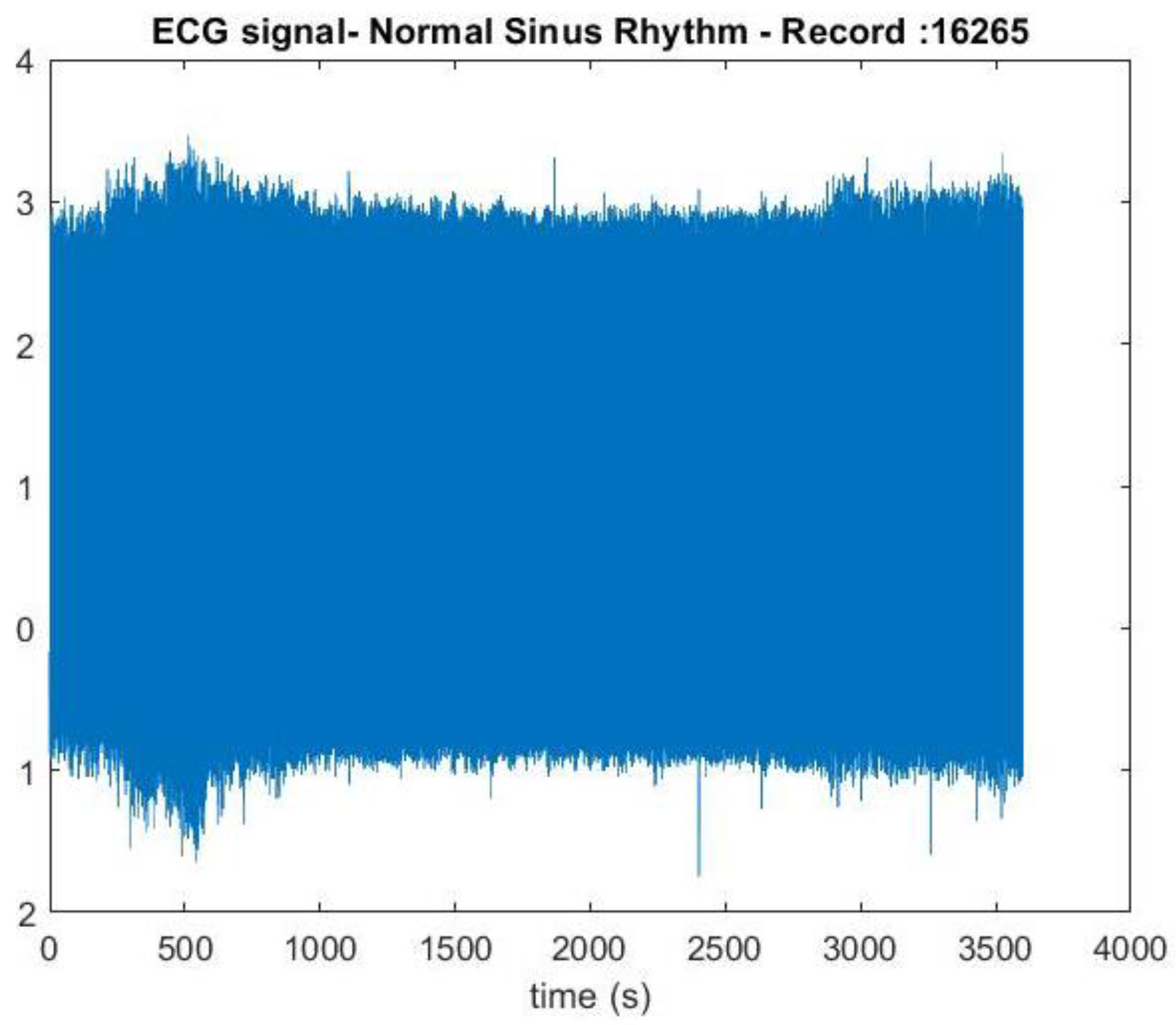
Figure 3.
Reconstructed signal containing R peaks in red color annotations of record no 16265.
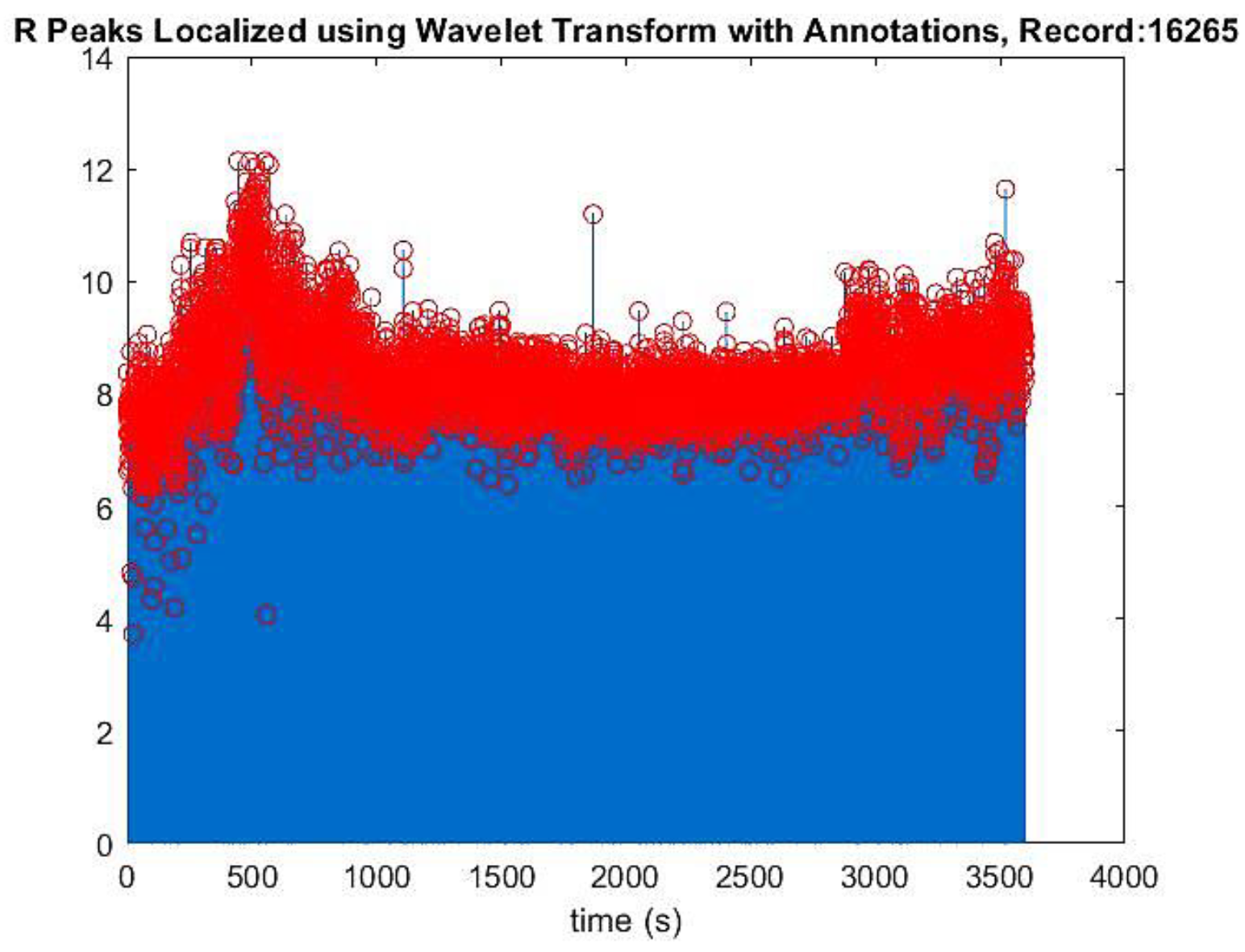
Figure 4.
The graph of RR intervals vs beat number. This is the representation of variation of the heart rate, HRV.
Figure 4.
The graph of RR intervals vs beat number. This is the representation of variation of the heart rate, HRV.
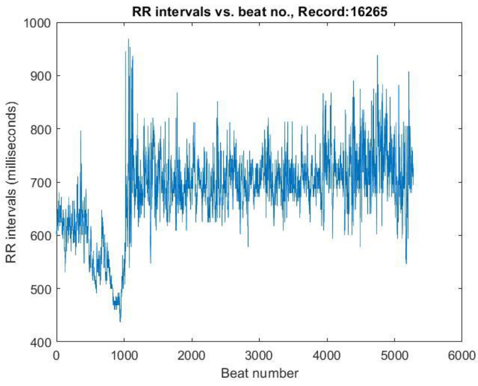
Figure 5.
The CWT spectrogram of record no 16265. CWT spectrum represents 3 dimensions; frequency, time and the RR interval magnitude by each coordinate. The dash line is cone of influence which indicates the more accurate results inside the cone. We can observe high magnitude events in bright colors in spectrograms.
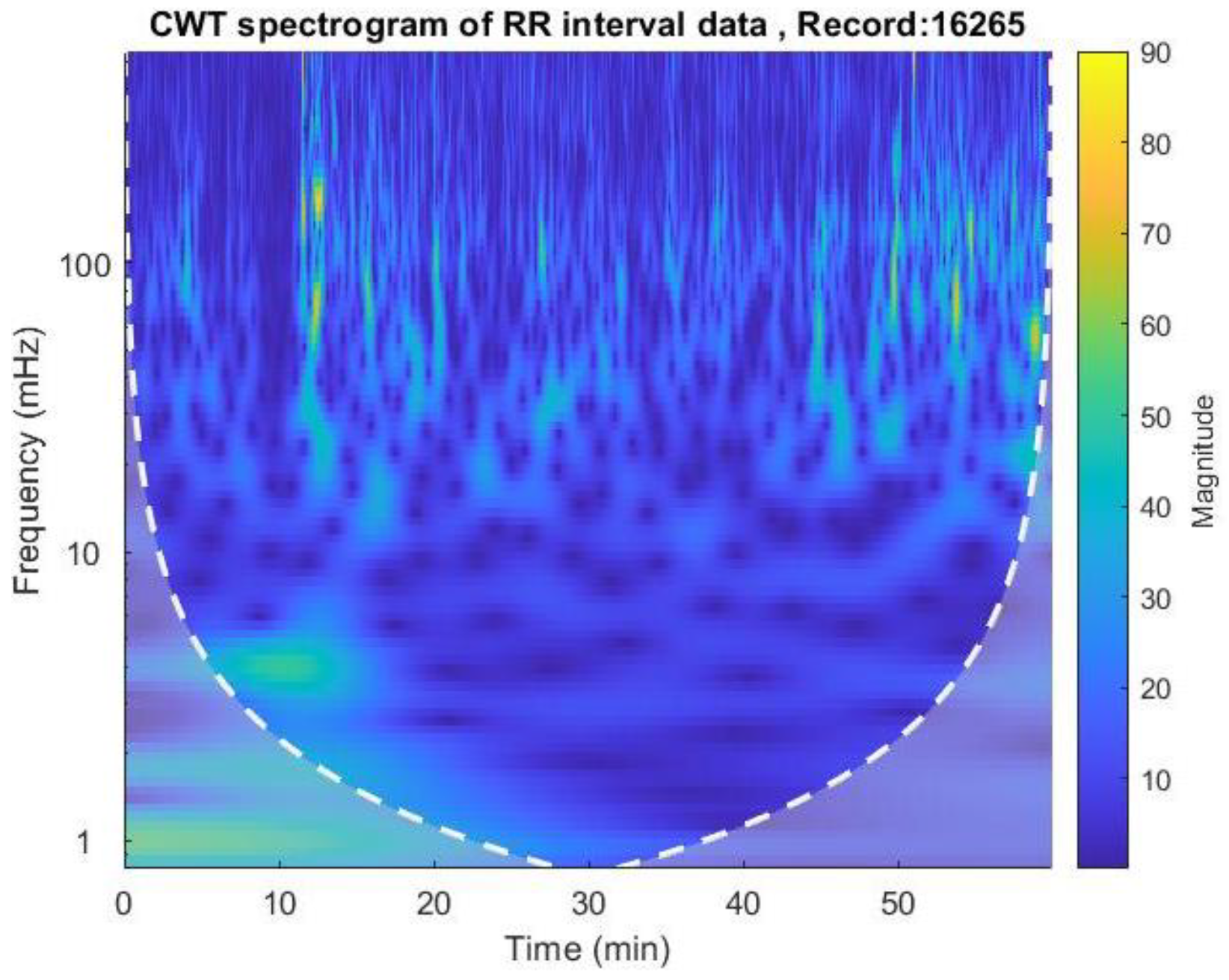
Figure 7.
(a) Located R peaks Figure 7. (b) RR interval vs beat no. plot Figure 7. (c) CWT Spectrogram for record:16786 using MODWPT.
Figure 7.
(a) Located R peaks Figure 7. (b) RR interval vs beat no. plot Figure 7. (c) CWT Spectrogram for record:16786 using MODWPT.
Figure 8.
(a) Located R peaks, Figure 8. (b) RR interval vs beat no. plot Figure 8. (c) CWT Spectrogram for record:16786 using MODWT. For recording no 16786 MODWPT method and MODWT method does not show any significant difference.
Figure 8.
(a) Located R peaks, Figure 8. (b) RR interval vs beat no. plot Figure 8. (c) CWT Spectrogram for record:16786 using MODWT. For recording no 16786 MODWPT method and MODWT method does not show any significant difference.
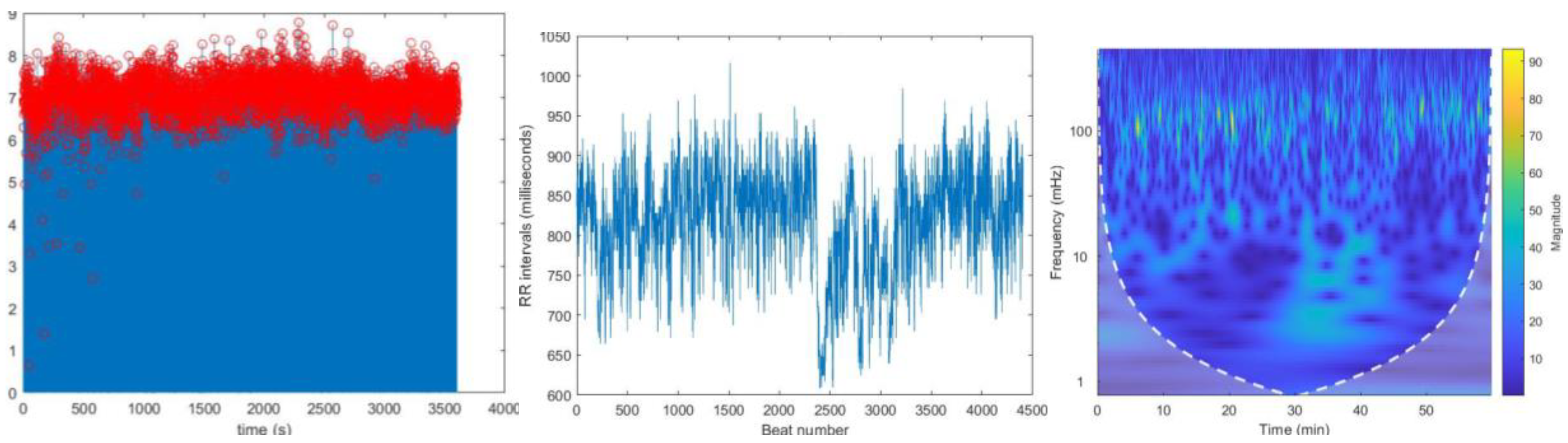
Figure 9.
(a) Located R peaks, Figure 9. (b) RR interval vs beat no. plot Figure 9.(c) CWT Spectrogram for record:117 using MODWPT. When comparing these plots with the MODWT method plots we can observe a significant difference in HF range until 600 beat number.
Figure 9.
(a) Located R peaks, Figure 9. (b) RR interval vs beat no. plot Figure 9.(c) CWT Spectrogram for record:117 using MODWPT. When comparing these plots with the MODWT method plots we can observe a significant difference in HF range until 600 beat number.
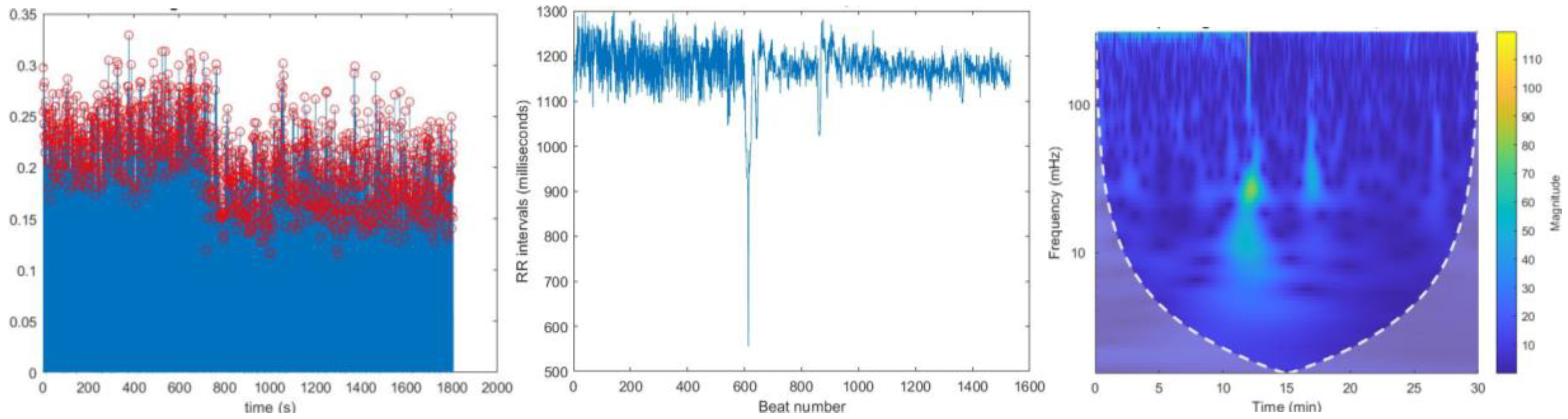
Figure 10.
(a) Located R peaks Figure 10. (b) RR interval vs beat no. plot Figure 10. (c) CWT Spectrogram for record:117 using MODWT.
Figure 10.
(a) Located R peaks Figure 10. (b) RR interval vs beat no. plot Figure 10. (c) CWT Spectrogram for record:117 using MODWT.
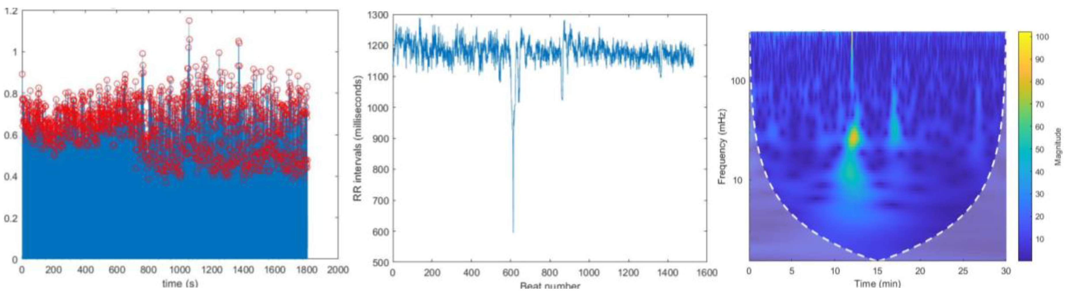
Figure 11.
Missing peaks observed in the R peaks plot of recording: Figure 11. (a) 16420 Figure 11. (b) 16483 Figure 11. (c) 101 Figure 11. (d) 111 Figure 11. (e) 121 and Figure 11. (f) 234. These plots shows the missed R peak circled in yellow color.
Figure 11.
Missing peaks observed in the R peaks plot of recording: Figure 11. (a) 16420 Figure 11. (b) 16483 Figure 11. (c) 101 Figure 11. (d) 111 Figure 11. (e) 121 and Figure 11. (f) 234. These plots shows the missed R peak circled in yellow color.
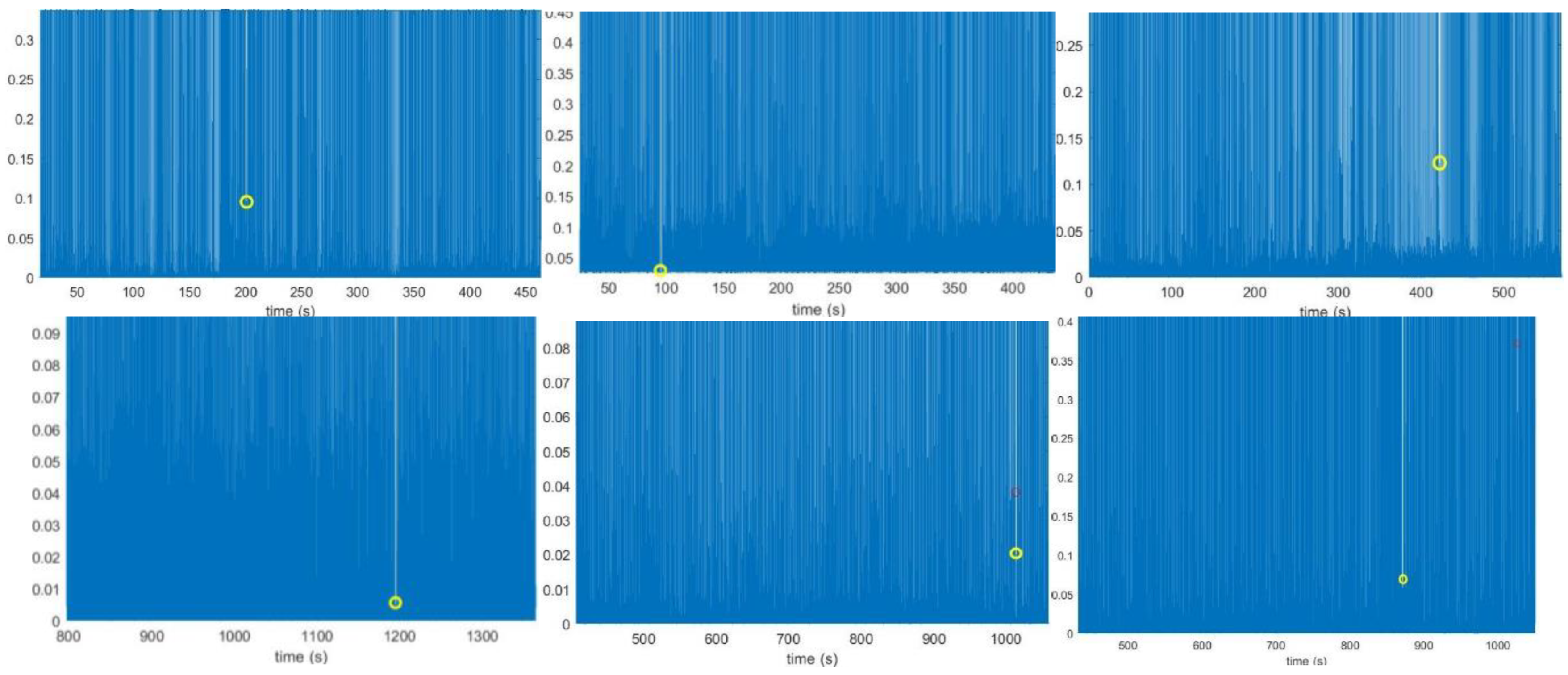
Figure 12.
The RR interval plot of recording: Figure 12. (a) 16420 observed with an incorrect higher interval between R peaks Figure 12. (b) 16420 obtained from PhysioNet Database Figure 12. (c) 121 observed with an incorrect higher interval between R peaks Figure 12. (d) 121 obtained from PhysioNet Database.
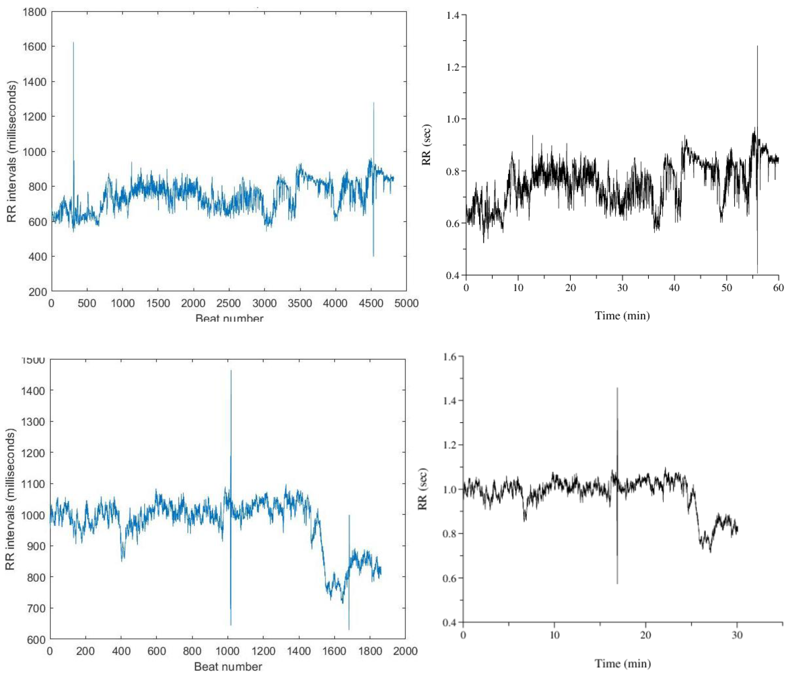
Figure 13.
(a) RR interval plot of Recording 16786 Plotted using MATLAB Figure 13. (b) RR interval plot of Recording 16786 Obtained from PhysioBank ATM Figure 13 (c) RR interval plot of Recording 230 Plotted using MATLAB Figure 12. (d) RR interval plot of Recording 230 Obtained from PhysioBank ATM.
Figure 13.
(a) RR interval plot of Recording 16786 Plotted using MATLAB Figure 13. (b) RR interval plot of Recording 16786 Obtained from PhysioBank ATM Figure 13 (c) RR interval plot of Recording 230 Plotted using MATLAB Figure 12. (d) RR interval plot of Recording 230 Obtained from PhysioBank ATM.
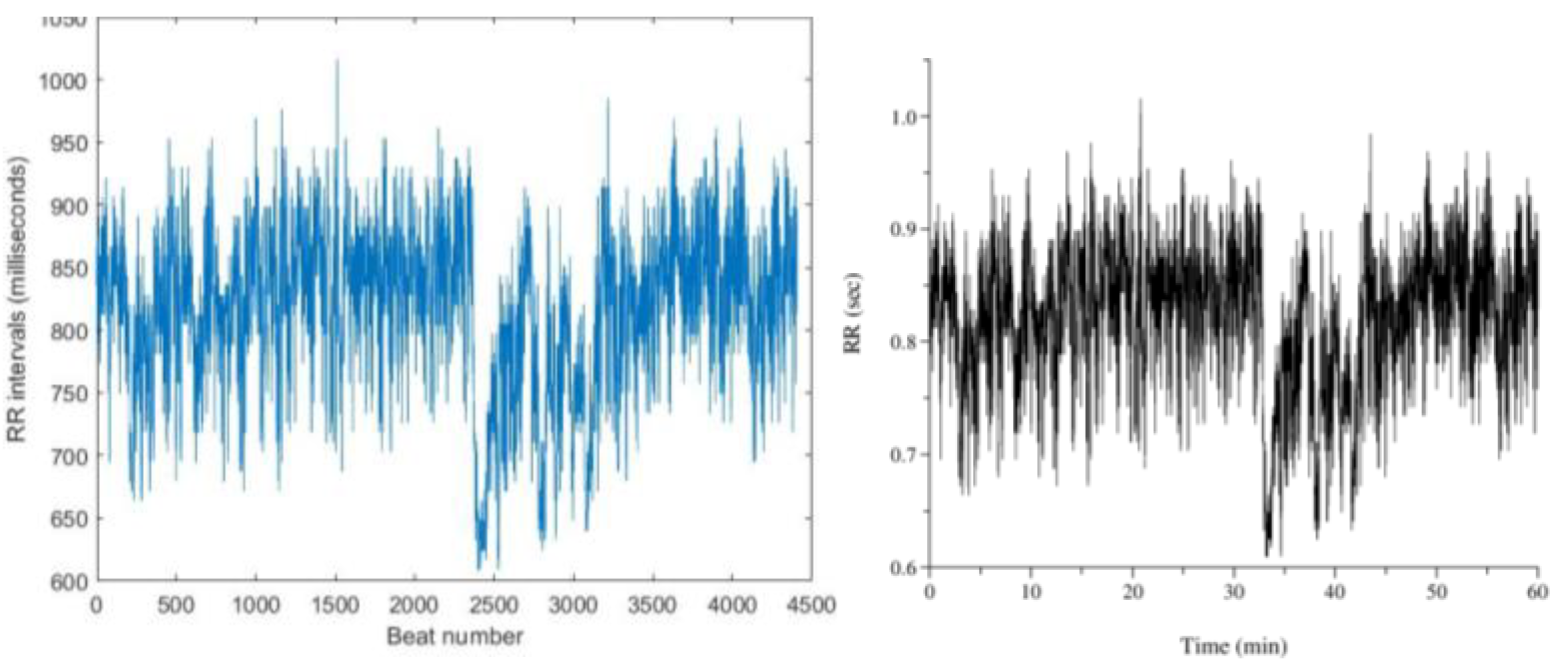
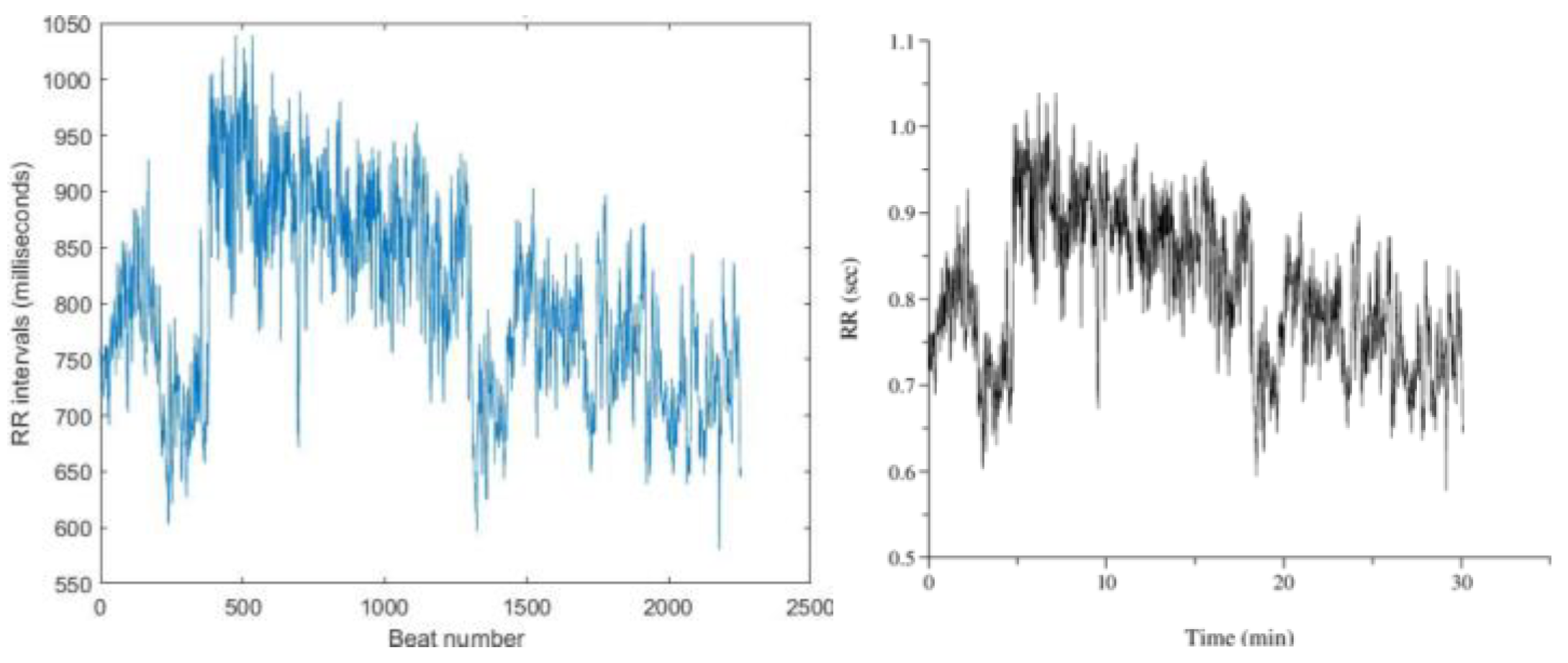
Figure 14.
(a) RR interval plot of Recording no. 16773 Plotted using MATLAB Figure 14. (b) RR interval plot of Recording no. 16773 obtained from PhysioBank ATM.
Figure 14.
(a) RR interval plot of Recording no. 16773 Plotted using MATLAB Figure 14. (b) RR interval plot of Recording no. 16773 obtained from PhysioBank ATM.
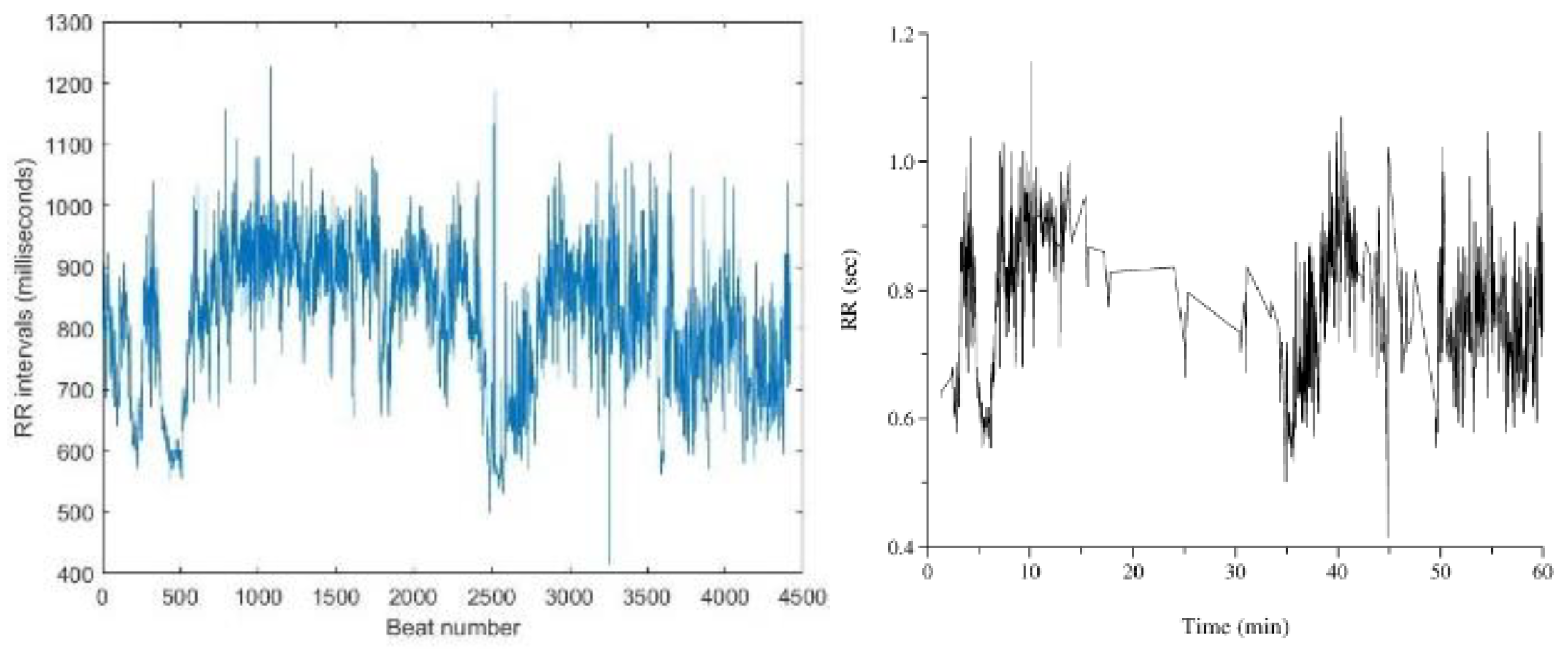
Figure 15.
CWT Spectrograms of Recording no. Figure 15. (a) 19093 Figure 15. (b) 228.
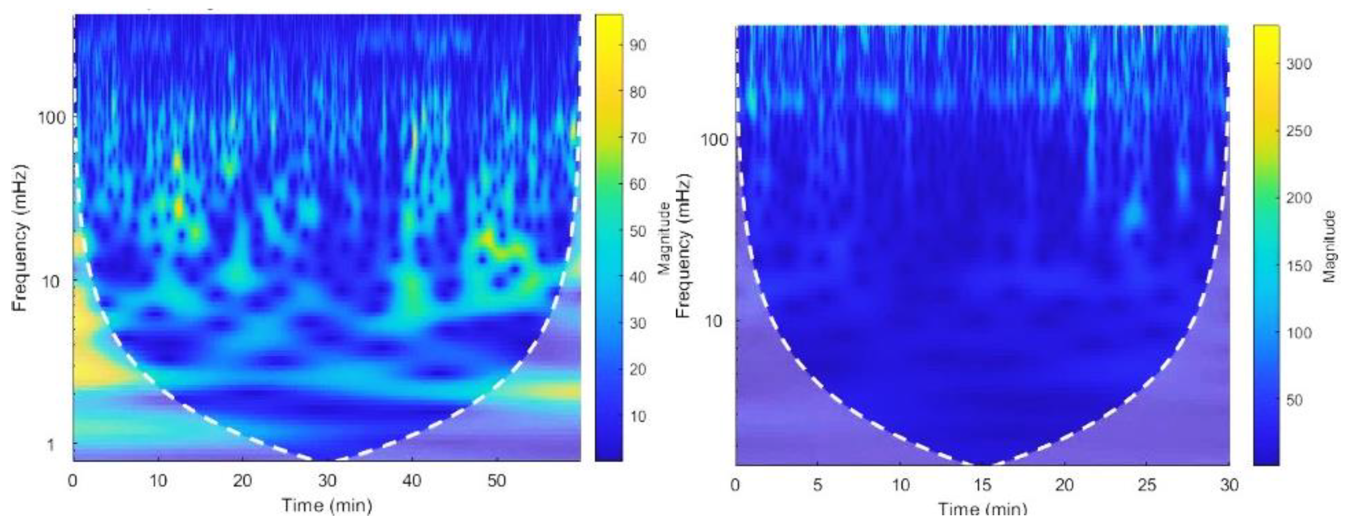
Figure 16.
RR intervals vs beat no. plots of Recording no. Figure 16. (a) 112 Figure 16. (b) 123 Figure 16. (c) 222.
Figure 16.
RR intervals vs beat no. plots of Recording no. Figure 16. (a) 112 Figure 16. (b) 123 Figure 16. (c) 222.
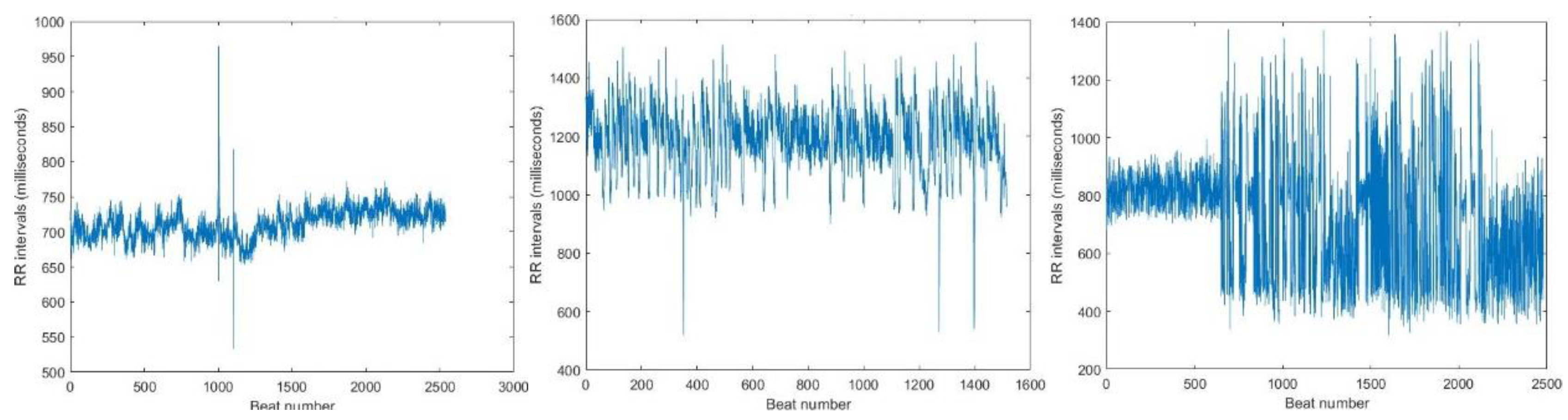
Figure 17.
CWT Spectrograms of Recording no. Figure 17. (a) 112 Figure 17. (b) 123 Figure 17. (c) 222.
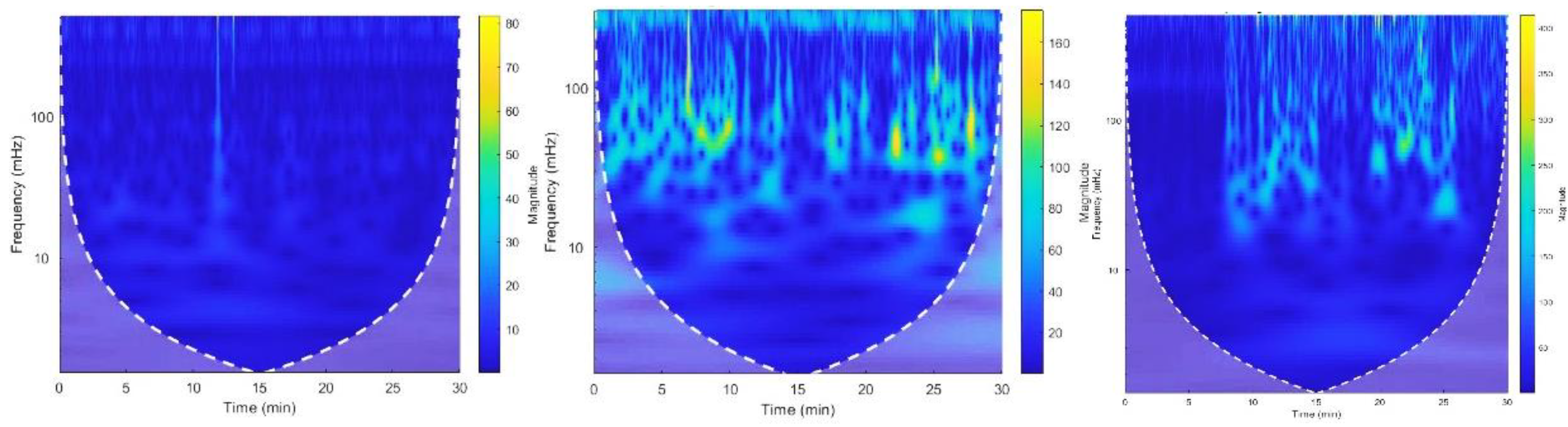
Figure 18.
(a) CWT Spectrograms and Figure 18. (b) RR intervals vs beat no. plots of Recording no.16539.
Figure 18.
(a) CWT Spectrograms and Figure 18. (b) RR intervals vs beat no. plots of Recording no.16539.
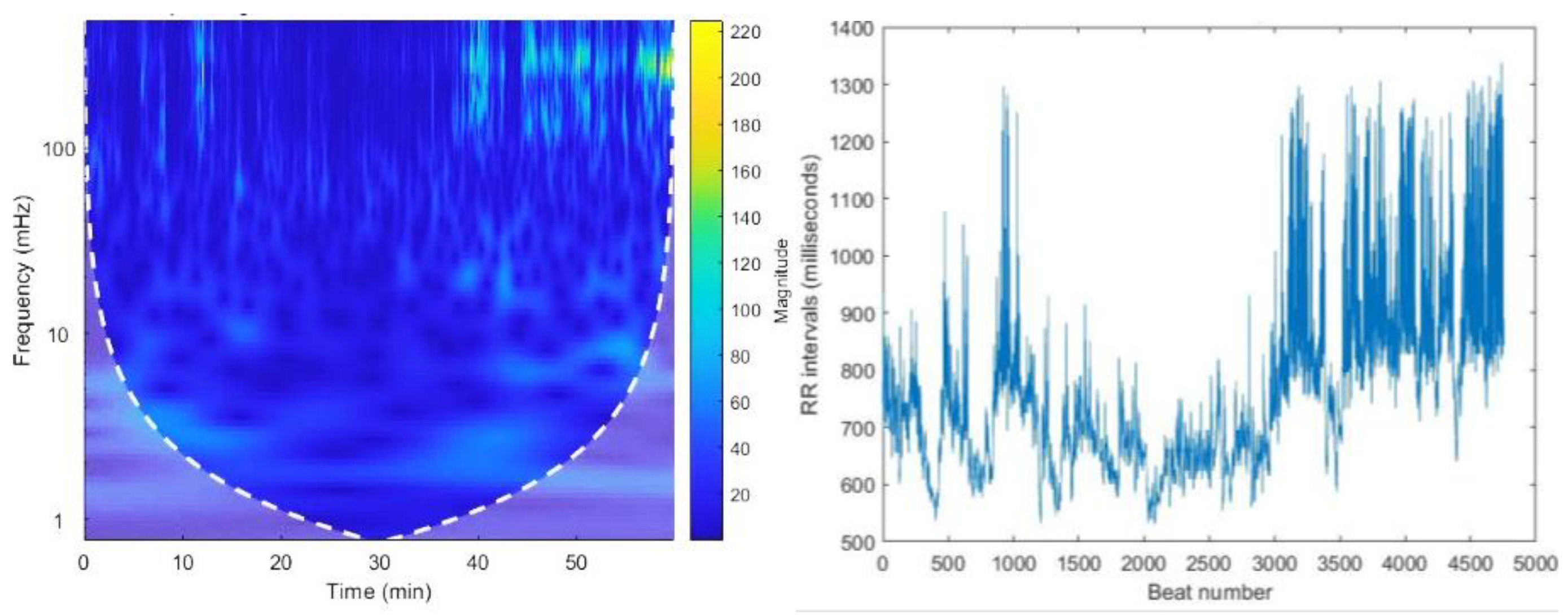
Figure 19.
CWT Spectrograms of Recording No. 121.
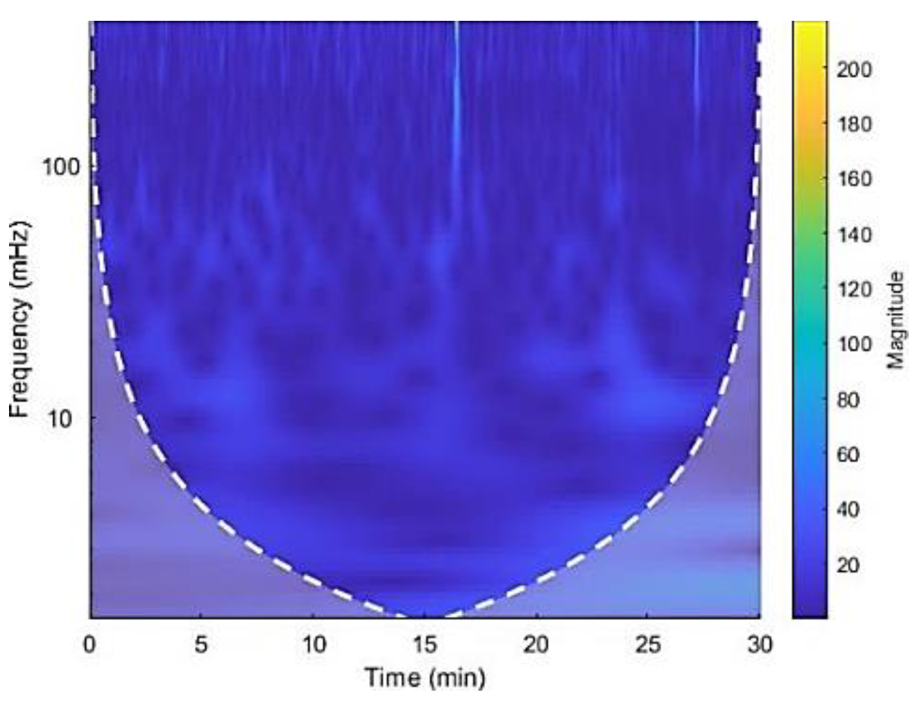
Figure 20.
CWT Spectrograms of Recording no. Figure 20. (a) 122 Figure 20. (b) 205.
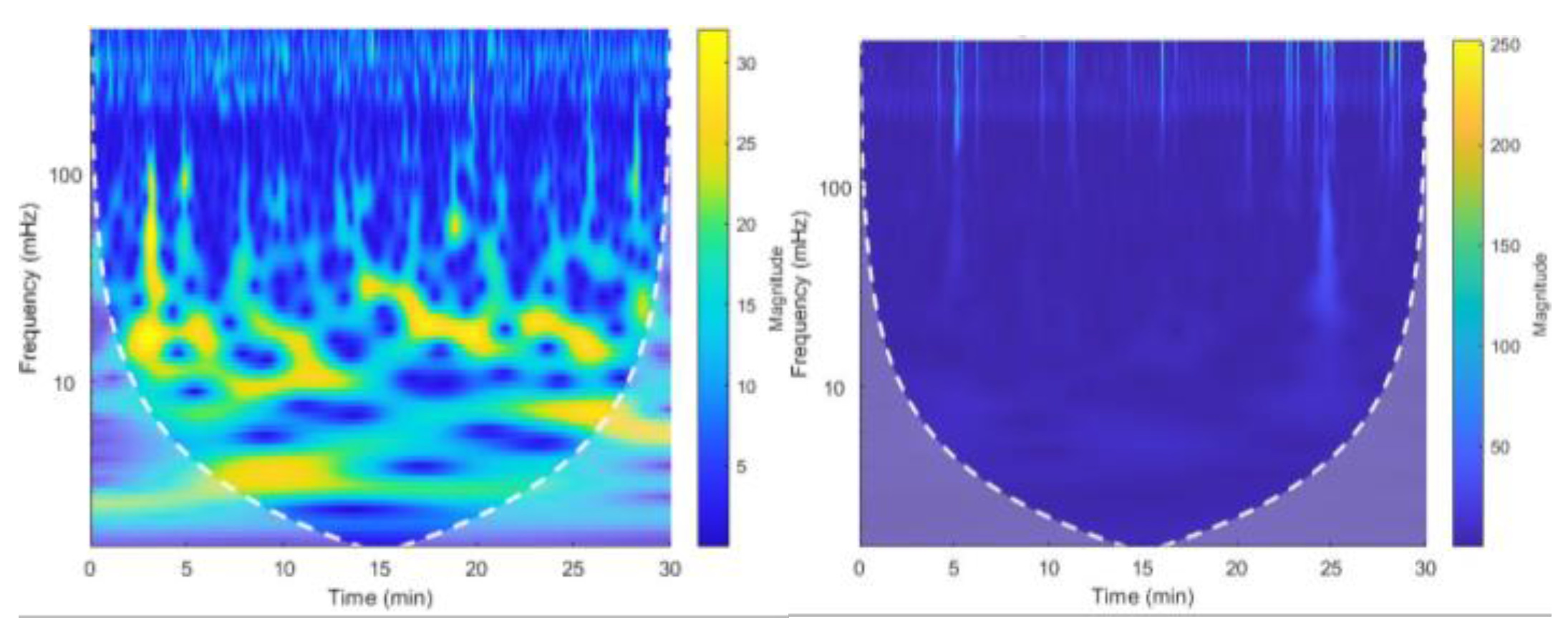
Figure 21.
CWT Spectrograms of Recording no. Figure 21. (a) 106 Figure 21. (b) 119 Figure 21. (c) 233.
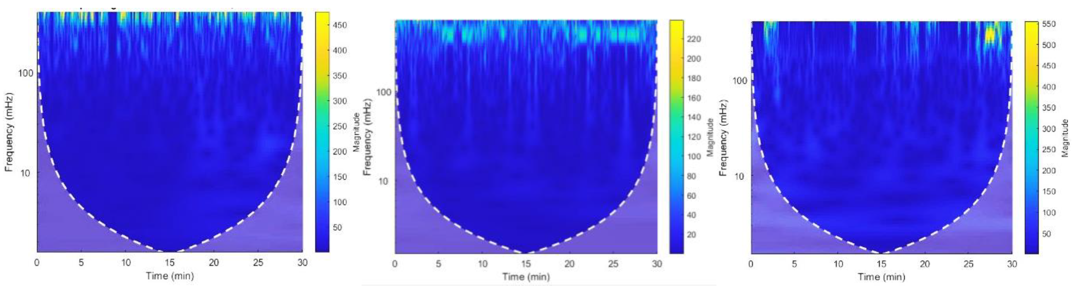
Figure 22.
RR intervals vs beat number plots of Recording no. Figure 22. (a) 106 Figure 22. (b) 119 Figure 22. (c) 233.
Figure 22.
RR intervals vs beat number plots of Recording no. Figure 22. (a) 106 Figure 22. (b) 119 Figure 22. (c) 233.
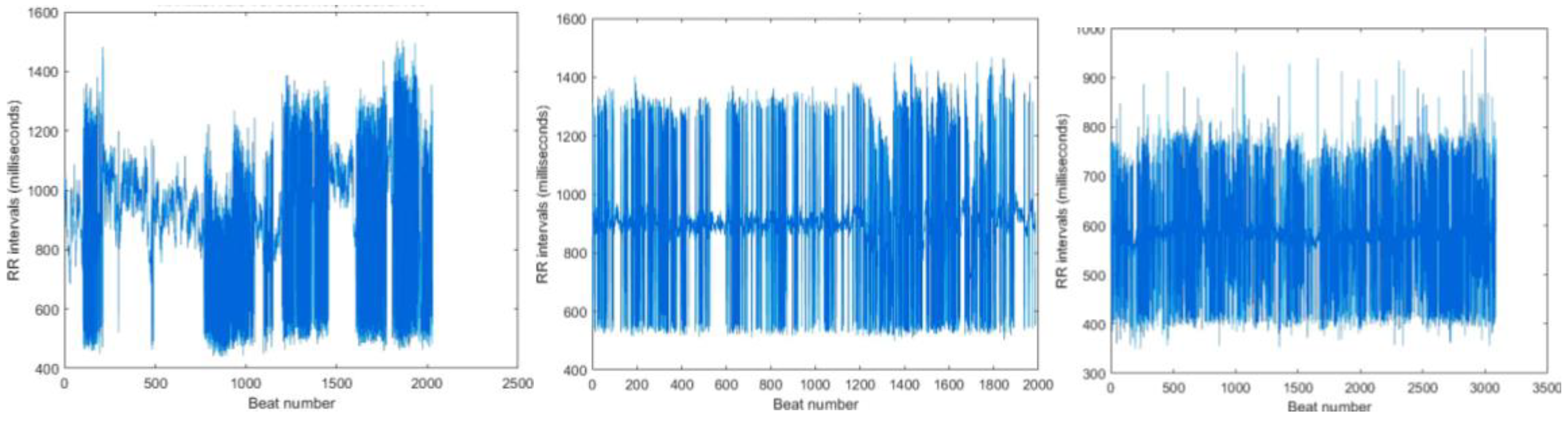
Figure 23.
Scatter plot of LF/HF values of Figure 23.(a) Normal Sinus Rhythm dataset Figure 23. (b) Arrhythmia dataset.
Figure 23.
Scatter plot of LF/HF values of Figure 23.(a) Normal Sinus Rhythm dataset Figure 23. (b) Arrhythmia dataset.
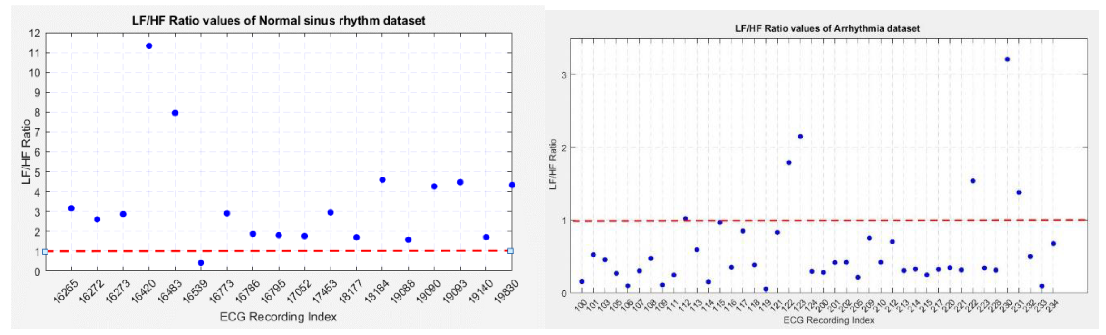
Table 1.
Frequency ranges for each level in DWT (Sampling frequency 128Hz).
| Level | Scale | Frequency Band (Hz) |
|---|---|---|
| 1 | 2 | 64-128 |
| 2 | 4 | 32-64 |
| 3 | 8 | 16-32 |
| 4 | 16 | 8-16 |
| 5 | 32 | 4-8 |
Table 2.
Frequency ranges for each level in DWT (Sampling frequency 360Hz).
| Level | Scale | Frequency Band (Hz) |
|---|---|---|
| 1 | 2 | 90-180 |
| 2 | 4 | 45-90 |
| 3 | 8 | 22.5-45 |
| 4 | 16 | 11.25-22.5 |
| 5 | 32 | 5.625-11.25 |
| 6 | 64 | 2.8125-5.625 |
Table 3.
Estimated LF/HF ratio values using MODWPT and MODWT methods.
| LF/HF ratio | ||||||
|---|---|---|---|---|---|---|
| Index | 16265 | 16786 | 19140 | 106 | 112 | 117 |
| Method | ||||||
| MODWPT | 3.188 | 1.869 | 1.682 | 0.103 | 1.032 | 0.424 |
| MODWT | 3.164 | 1.875 | 1.700 | 0.098 | 1.028 | 0.852 |
Disclaimer/Publisher’s Note: The statements, opinions and data contained in all publications are solely those of the individual author(s) and contributor(s) and not of MDPI and/or the editor(s). MDPI and/or the editor(s) disclaim responsibility for any injury to people or property resulting from any ideas, methods, instructions or products referred to in the content. |
© 2025 by the authors. Licensee MDPI, Basel, Switzerland. This article is an open access article distributed under the terms and conditions of the Creative Commons Attribution (CC BY) license (http://creativecommons.org/licenses/by/4.0/).
Copyright: This open access article is published under a Creative Commons CC BY 4.0 license, which permit the free download, distribution, and reuse, provided that the author and preprint are cited in any reuse.


