A Short Note on Gaussian Distribution with Non-Constant Correlation

1. Background

Gaussian copula is widely used in quantitative finance modelling. The Gaussian distribution is closely related to an underlying Brownian motion: the standard multi-variate normal distribution is the terminal distribution of an underlying multi-variate Brownian motion where the correlations are constant over time. However the correlation being constant is a limitation of this model which might not fit the actual market. On the other hand, if the correlations are not constant, the result terminal distribution has no closed-form representation in general. Without the closed-form solution or analytic tractability, it becomes less attractive for practical usage. There are research in alternative directions which bypass this tractability issue, for example in (Lucic 2012; Luján 2022), the respective authors created different terminal distributions which can admit shape with the desired correlation skew effect. In this paper, we still focus on the terminal distribution result from the Brownian motion itself. We study the PDE for the density function and show that with some assumption on the correlation function, we can derive some PDEs which can describe the moments of the marginal and conditional distributions. In particular, these PDEs are of lower dimensions, therefore the calculations are fast and practical. With these moments, we can generate moment matching approximations with nice analytic tractability to the true terminal distribution. The result analytic distribution can be a useful variation to the standard multi-variate normal distribution and it can be used for purpose like modelling correlation skew effect in quant finance.

2. Methodology

2.1. Model Setup

We study this math problem below. This is a 2-dimensional case however we show later that similar techniques can be applied to higher dimensions.

$$\begin{array}{ccc}\hfill x(0),y(0)& =& 0,0\hfill \end{array}$$

(1)

$$\begin{array}{ccc}\hfill dx& =& d{w}_1\hfill \end{array}$$

(2)

$$\begin{array}{ccc}\hfill dy& =& \rho (x,y,t)d{w}_1+\sqrt{1-{\rho }^2(x,y,t)}d{w}_2\hfill \end{array}$$

(3)

$$\begin{array}{ccc}\hfill <d{w}_1,d{w}_2>& =& 0\hfill \end{array}$$

(4)

The Fokker-Planck equation (Fokker 1914; Kolmogorov 1931; Planck 1917) describes the joint probability density function $p(x,y,t)$ by:

$${\displaystyle \frac{\mathit{\partial }p}{\mathit{\partial }t}}={\displaystyle \frac{1}{2}}({\displaystyle \frac{\mathit{\partial }p}{\mathit{\partial }{x}^2}}+2{\displaystyle \frac{\mathit{\partial }(\rho p)}{\mathit{\partial }x\mathit{\partial }y}}+{\displaystyle \frac{\mathit{\partial }p}{\mathit{\partial }{y}^2}})$$

(5)

This is a 2d-PDE in the convention of quant finance industry (2d refers to 2-dimension in space variables $(x,y)$ while in fact it is a 3-d PDE if counting t, given the common presence of t in this type of PDE we refer the dimensions to only the space variables) and the general numerical method is slow. However, we can reduce the complexity of the 2d-PDE if we make a reasonable assumtion on the correlation function as below:

$$\rho (x,y,t)=\rho (x+y,t)$$

(6)

This means the correlation depends on the $(x,y)$ in terms of the total $(x+y)$, which can be interpreted as: correlation depends on a market factor which is the average of the underlyers. With this extra assumption, we can simplify the problem as below:

Lets make change of variables below

$$\begin{array}{ccc}\hfill u& =& {\displaystyle \frac{1}{2}}(x+y)\hfill \end{array}$$

(7)

$$\begin{array}{ccc}\hfill v& =& {\displaystyle \frac{1}{2}}(x-y)\hfill \end{array}$$

(8)

Then we have

$$<du,dv>={\displaystyle \frac{1}{4}}(<dx,dx>-<dy,dy>)=0$$

(9)

And $du,dv$ can be written as

$$\begin{array}{ccc}\hfill du& =& \sqrt{{\displaystyle \frac{1+\rho (u,t)}{2}}}d{w}_3\hfill \end{array}$$

(10)

$$\begin{array}{ccc}\hfill dv& =& \sqrt{{\displaystyle \frac{1-\rho (u,t)}{2}}}d{w}_4\hfill \end{array}$$

(11)

Note the first diffusion only involves u, then Fokker-Planck equation for probability density of u is a 1d-PDE:

$${\displaystyle \frac{\mathit{\partial }p(u,t)}{\mathit{\partial }t}}={\displaystyle \frac{1}{2}}{\displaystyle \frac{{\mathit{\partial }}^2}{\mathit{\partial }{u}^2}}({\displaystyle \frac{1+\rho (u,t)}{2}}p(u,t))$$

(12)

So we can solve $p(u,t)$ first, then we look at the $v(t)$. For any given path $u(s),0\le s\le t$, the $v(t)$ is simply a sum of infinitesimal normal variables with variances ${\displaystyle \frac{1-\rho (u(s),s)}{2}}$, so we know the distrubtion of $v(t)$ condition on this path $u(s),0\le s\le t$ is a normal distribution with mean 0 and variance

$${\int }_0^t{\displaystyle \frac{1-\rho (u(s),s)}{2}}ds$$

(13)

2.1.1. Conditional Distribution and the First Two Moments

Conditioned on a path is not easy to use for calculation, it would be more useful to condition on a value $u(t)$ instead of the whole path. Let $\{v(t)|u(t)=u\}$ be the conditional distribution, note this distribution is not a strict normal distribution in general. A more detailed discussion of this distribution is left to later and now we focus on the first two moments, ie, the mean and variance of this conditional distribution.

The mean is clearly zero by symmetry. For the variance, denoted as $f(u,t)$, we have

Theorem 1.

Let $\{v(t)|u(t)=u\}$ be the conditional distribution of $v(t)$ conditioned on $u(t)=u$, then its variance $f(u,t)$ satisfy

$$f(u,t)=E[{\int }_0^t{\displaystyle \frac{1-\rho (u(s),s)}{2}}ds|u(t)=u]$$

(14)

Proof. 

The proof is straightforward. For completeness included below: By the stochastic integral definition as limit of sums, $v(t)|u(t)=u$ is the following sum with the constraint $u(t)=u$:

$$\sum _i\sqrt{{\displaystyle \frac{1-\rho (u_i,s_i)}{2}}}{\Delta }_i{w}_4$$

(15)

Using definition of variance, we get this sum

$$\sum _{i,j}\sqrt{{\displaystyle \frac{1-\rho (u_i,s_i)}{2}}}\sqrt{{\displaystyle \frac{1-\rho (u_j,s_j)}{2}}}{\Delta }_i{w}_4{\Delta }_j{w}_4$$

(16)

Which only has non-zero terms as below after taking expectation.

$$\sum _i{\displaystyle \frac{1-\rho (u_i,s)}{2}}{\Delta }_{i}t$$

(17)

with the constraint $u(t)=u$.

Then take the limit of ${\Delta }_{i}t\to 0$ and the statement is proven. □

Note $f(u,t)$ is a path integral on all possible paths $u(s)$ that get to u at t. We have the following:

$$p(u,t+dt)f(u,t+dt)={\int }_{-\infty }^{\infty }p(x,t)[f(x,t)+dt{\displaystyle \frac{1-\rho (x,t)}{2}}]p(u,t+dt|x,t)dx$$

(18)

The $p(u,t+dt|x,t)$ is the transition probability from state $(x,t)$ to $(u,t+dt)$.

Now we follow the Fokker-Planck equation derivation technique, we will get:

Theorem 2.

$${\displaystyle \frac{\mathit{\partial }}{\mathit{\partial }t}}(pf)=p{\displaystyle \frac{1-\rho (u,t)}{2}}+{\displaystyle \frac{1}{2}}{\displaystyle \frac{\mathit{\partial }}{\mathit{\partial }{u}^2}}(pf{\displaystyle \frac{1+\rho (u,t)}{2}})$$

(19)

Proof. 

$$\begin{array}{ccc}& & {\displaystyle \frac{\mathit{\partial }}{\mathit{\partial }t}}(pf)\hfill \\ & =& \underset{dt\to 0}{lim}{\displaystyle \frac{p(u,t+dt)f(u,t+dt)-p(u,t)f(u,t)}{dt}}\hfill \\ & =& \underset{dt\to 0}{lim}{\displaystyle \frac{{\int }_{-\infty }^{\infty }p(x,t)f(x,t)p(u,t+dt|x,t)dx-p(u,t)f(u,t)}{dt}}+\underset{dt\to 0}{lim}{\int }_{-\infty }^{\infty }p(x,t){\displaystyle \frac{1-\rho (x,t)}{2}}p(u,t+dt|x,t)dx\hfill \end{array}$$

Note the second term comes to

$$\underset{dt\to 0}{lim}{\int }_{-\infty }^{\infty }p(x,t){\displaystyle \frac{1-\rho (x,t)}{2}}p(u,t+dt|x,t)dx=p(u,t){\displaystyle \frac{1-\rho (u,t)}{2}}$$

So we just have to prove

$$\underset{dt\to 0}{lim}{\displaystyle \frac{{\int }_{-\infty }^{\infty }p(x,t)f(x,t)p(u,t+dt|x,t)dx-p(u,t)f(u,t)}{dt}}={\displaystyle \frac{1}{2}}{\displaystyle \frac{\mathit{\partial }}{\mathit{\partial }{u}^2}}(pf{\displaystyle \frac{1+\rho (u,t)}{2}})$$

Let $h(u)$ be a smooth function with compact support, consider

$$\begin{array}{ccc}& & {\int }_{-\infty }^{\infty }h(u){\int }_{-\infty }^{\infty }p(x,t)f(x,t)p(u,t+dt|x,t)dxdu\hfill \\ & =& {\int }_{-\infty }^{\infty }p(x,t)f(x,t){\int }_{-\infty }^{\infty }h(u)p(u,t+dt|x,t)dudx\hfill \\ & =& {\int }_{-\infty }^{\infty }p(x,t)f(x,t){\int }_{-\infty }^{\infty }(h(x)+h^{\prime }(u-x)+{\displaystyle \frac{1}{2}}{h}^{\prime \prime }{(u-x)}^2+O({(u-x)}^3))p(u,t+dt|x,t)dudx\hfill \end{array}$$

Now the integral ${\int }_{-\infty }^{\infty }{(u-x)}^{k}p(u,t+dt|x,t)du$ is the $k-th$ moment of the Brownian motion $du=\sqrt{{\displaystyle \frac{1+\rho (u,t)}{2}}}d{w}_3$, so we have

$$\begin{array}{ccc}\hfill {\int }_{-\infty }^{\infty }(u-x)p(u,t+dt|x,t)du& =& 0\hfill \\ \hfill {\int }_{-\infty }^{\infty }{(u-x)}^{2}p(u,t+dt|x,t)du& =& {\displaystyle \frac{1+\rho (x,t)}{2}}dt\hfill \\ \hfill {\int }_{-\infty }^{\infty }{(u-x)}^{k}p(u,t+dt|x,t)du& =& \mathrm{higher}\mathrm{order}\mathrm{than}dt\mathrm{when}k>2\hfill \end{array}$$

Then we have below, in the order of $dt$

$$\begin{array}{ccc}& & {\int }_{-\infty }^{\infty }h(u){\int }_{-\infty }^{\infty }p(x,t)f(x,t)p(u,t+dt|x,t)dxdu\hfill \\ & =& {\int }_{-\infty }^{\infty }p(x,t)f(x,t)h(x){\int }_{-\infty }^{\infty }p(u,t+dt|x,t)dudx+dt{\int }_{-\infty }^{\infty }{\displaystyle \frac{1}{2}}p(x,t)f(x,t)h^{\prime \prime }{\displaystyle \frac{1+\rho (x,t)}{2}}dx\hfill \\ & =& {\int }_{-\infty }^{\infty }p(x,t)f(x,t)h(x)dx+dt{\int }_{-\infty }^{\infty }{\displaystyle \frac{1}{2}}p(x,t)f(x,t)h^{\prime \prime }{\displaystyle \frac{1+\rho (x,t)}{2}}dx\hfill \end{array}$$

so

$$\begin{array}{ccc}& & \underset{dt\to 0}{lim}{\displaystyle \frac{{\int }_{-\infty }^{\infty }h(u){\int }_{-\infty }^{\infty }p(x,t)f(x,t)p(u,t+dt|x,t)dxdu-{\int }_{-\infty }^{\infty }h(u)p(u,t)f(u,t)du}{dt}}\hfill \\ & =& {\int }_{-\infty }^{\infty }{\displaystyle \frac{1}{2}}p(x,t)f(x,t)h^{\prime \prime }{\displaystyle \frac{1+\rho (x,t)}{2}}dx\hfill \\ & =& {\int }_{-\infty }^{\infty }h(x){\displaystyle \frac{1}{2}}{\displaystyle \frac{{\mathit{\partial }}^2}{\mathit{\partial }{x}^2}}(p(x,t)f(x,t){\displaystyle \frac{1+\rho (x,t)}{2}})dx\hfill \end{array}$$

The last step in above is integration by parts. Because the $h(u)$ is arbitrary smooth function so it follows that:

$$\underset{dt\to 0}{lim}{\displaystyle \frac{{\int }_{-\infty }^{\infty }p(x,t)f(x,t)p(u,t+dt|x,t)dx-p(u,t)f(u,t)}{dt}}={\displaystyle \frac{1}{2}}{\displaystyle \frac{\mathit{\partial }}{\mathit{\partial }{u}^2}}(pf{\displaystyle \frac{1+\rho (u,t)}{2}})$$

  □

To recap, we have these 2 key equations:

$$\begin{array}{ccc}\hfill {\displaystyle \frac{\mathit{\partial }p(u,t)}{\mathit{\partial }t}}& =& {\displaystyle \frac{1}{2}}{\displaystyle \frac{{\mathit{\partial }}^2}{\mathit{\partial }{u}^2}}({\displaystyle \frac{1+\rho (u,t)}{2}}p(u,t))\hfill \end{array}$$

(20)

$$\begin{array}{ccc}\hfill {\displaystyle \frac{\mathit{\partial }}{\mathit{\partial }t}}(pf)& =& p{\displaystyle \frac{1-\rho (u(t),t)}{2}}+{\displaystyle \frac{1}{2}}{\displaystyle \frac{\mathit{\partial }}{\mathit{\partial }{u}^2}}(pf{\displaystyle \frac{1+\rho (u,t)}{2}})\hfill \end{array}$$

(21)

We can solve for p first and then solve for f (It is also possible to bundle the PDE solving for p and f together in discretization etc). Knowing $p(u,t)$ and $f(u,t)$, we know the marginal distribution of u and the mean (0) and variance of the conditional distribution $\{v(t)|u(t)=u\}$. Note we mentioned previously the conditional distribution $\{v(t)|u(t)=u\}$ is not strictly normal in general: A sample of it is basicly a two step process: first choose a path for u subject to the $u(t)$ terminal condition, this yields a path-wise integral ${\int }_0^t{\displaystyle \frac{1-\rho (u,s)}{2}}ds$. Then choose a point from a normal distribution with variance set to ${\int }_0^t{\displaystyle \frac{1-\rho (u,s)}{2}}ds$. Or one can also think it as first choose a sample from a standard normal distribution, then choose a path for u subject to the terminal condition, calculate the $\sqrt{{\int }_0^t{\displaystyle \frac{1-\rho (u,s)}{2}}ds}$ and scale the normal variable with it.

One might think the 2nd view can keep the normal ness of the whole sampling result, but actually not: some heriustic thinking is that the normal sampling tends to be centralized, and then the scaling also has some centralized tendency, therefore not the same as a constant scaling will do. This is heriustic of course, but next we develope equations for higher moment, then one can see it won’t be a strict normal as the 4th moment vs 2nd moment relation is different to a normal distribution.

2.1.2. Higher Order Moments

We can derive the equations of the higher order moments following the similar technique. To demonstrate, we look at the 4-th order. Let $g(u,t)$ be the 4-th order moment of the conditional distribution $\{v(t)|u(t)=u\}$.

Theorem 3. 

$${\displaystyle \frac{\mathit{\partial }(pg)}{\mathit{\partial }t}}=3(1-\rho (u,t))pf+{\displaystyle \frac{1}{2}}{\displaystyle \frac{{\mathit{\partial }}^2}{\mathit{\partial }{u}^2}}(pg{\displaystyle \frac{1+\rho (u,t)}{2}})$$

(22)

Proof. 

4-th order moment is limit of sum below with constraint $u(t)=u$

$$\sum _{i,j,k,l}(\prod _{m\in \{i,j,k,l\}}\sqrt{{\displaystyle \frac{1-\rho (u_m,s_m)}{2}}}{\Delta }_{m}w)$$

(23)

After taking expectation and removing zero terms, this becomes below: note ($i=j$ terms are approaching to 0 when making finer grids so we ignored them)

$$6\sum _{i<j}{\displaystyle \frac{1-\rho (u_i,s_i)}{2}}{\displaystyle \frac{1-\rho (u_j,s_j)}{2}}{\Delta }_{i}t{\Delta }_{j}t$$

(24)

Taking limit, in integral representation, it is

$$g(u,t)=E[6{\int }_0^t{\displaystyle \frac{1-\rho (u(s),s)}{2}}ds{\int }_s^t{\displaystyle \frac{1-\rho (u(x),x)}{2}}dx|u(t)=u]$$

(25)

Then following the Fokker Planck derivation, we have:

$$p(u,t+dt)g(u,t+dt)={\int }_{-\infty }^{\infty }p(x,t)[g(x,t)+6dtf(x,t){\displaystyle \frac{1-\rho (x,t)}{2}}]p(u,t+dt|x,t)dx$$

(26)

The $p(u,t+dt|x,t)$ is the transition probability from state $(x,t)$ to $(u,t+dt)$. Then following the previous derivation we have

$${\displaystyle \frac{\mathit{\partial }(pg)}{\mathit{\partial }t}}=3(1-\rho (u,t))pf+{\displaystyle \frac{1}{2}}{\displaystyle \frac{{\mathit{\partial }}^2}{\mathit{\partial }{u}^2}}(pg{\displaystyle \frac{1+\rho (u,t)}{2}})$$

(27)

  □

Now we can prove the conditional distribution is not normal in general, because normal distribution’s 4th order moment is 3 times of the variance square.

Lemma 1. 

if $g=3f^2$, then ${\displaystyle \frac{\mathit{\partial }f}{\mathit{\partial }u}}=0$

Proof. 

Plug into the equations and straightforward. □

If ${\displaystyle \frac{\mathit{\partial }f}{\mathit{\partial }u}}=0$ then it becomes the standard multi-variate normal distribution.

2.1.3. Normal Approximation to the Conditional

With above in mind, we still prefer to use the normal distribution with the variance matching $f(u,t)$ to approximate the true conditional distribution. This is because first it can match the moments to the 2nd order which is usually good enough for many practical usage. Secondly, the normal distribution has very good analytic tractability.

Note that the normal distribution is not a random choice either: if we denote the true joint density as $p(u,t)q(u,v,t)$ where $q(u,v,t)$ is the conditional probability of v conditioned on u. Then when we use a normal density form for the q, it will satisfy the Fokker Planck equation on most of the terms.

This leads to a question: is there a good analytic form for the q such that it can match moments to higher order (for example 4-th order) ? Obviously such form will involve $f,g$ or the moments it need to match. Due to my limited knowledge, this remains interesting but also a mystery to me.

3. Higher Dimensions and General Form

In higher dimensions, similar technique can be applied if we assume the correlations are driven by one factor. Lets denote that factor as M, then by Cholesky decomposition, we can re-write the dynamics as following:

$$\begin{array}{ccc}\hfill dM& =& A(M,t)d{W}_1\hfill \end{array}$$

(28)

$$\begin{array}{ccc}\hfill d{X}_2& =& A_{21}(M,t)d{W}_1+A_{22}(M,t)d{W}_2\hfill \end{array}$$

(29)

$$\begin{array}{ccc}\hfill d{X}_3& =& A_{31}(M,t)d{W}_1+A_{32}(M,t)d{W}_2+A_{33}(M,t)d{W}_3\hfill \end{array}$$

(30)

$$\begin{array}{c}\hfill \cdots \end{array}$$

(31)

$$\begin{array}{ccc}\hfill d{X}_i& =& \sum _k{A}_{ik}d{W}_k\hfill \end{array}$$

(32)

$$\begin{array}{c}\hfill \cdots \end{array}$$

(33)

$d{W}_i$ are independent brownian motions. All the correlation terms only depend on M and t. We have following result:

Theorem 4. 

Let $p(M,t)$ be the probability density function for M at t, then

$${\displaystyle \frac{\mathit{\partial }p(M,t)}{\mathit{\partial }t}}={\displaystyle \frac{1}{2}}{\displaystyle \frac{\mathit{\partial }}{\mathit{\partial }{M}^2}}(A^{2}p)$$

(34)

Let $f_i(M,t)$ be the $E[X_i|M(t)=M]$, then

$${\displaystyle \frac{\mathit{\partial }(p{f}_i)}{\mathit{\partial }t}}=-{\displaystyle \frac{\mathit{\partial }}{\mathit{\partial }M}}(p{A}_{i1}A)+{\displaystyle \frac{1}{2}}{\displaystyle \frac{\mathit{\partial }}{\mathit{\partial }{M}^2}}(A^{2}p{f}_i)$$

(35)

Let $g_{ij}(M,t)$ be the $E[X_i{X}_j|M(t)=M]$, then

$${\displaystyle \frac{\mathit{\partial }(p{g}_{ij})}{\mathit{\partial }t}}=p\sum _{k\le min(i,j)}{A}_{ik}{A}_{jk}-{\displaystyle \frac{\mathit{\partial }}{\mathit{\partial }M}}(p{f}_i{A}_{j1}A+p{f}_j{A}_{i1}A)+{\displaystyle \frac{1}{2}}{\displaystyle \frac{\mathit{\partial }}{\mathit{\partial }{M}^2}}(A^{2}p{g}_{ij})$$

(36)

Proof. 

Standard Fokker Planck derivation using Taylor expansions and integration by parts. Similar to previous one in 2-d case. □

These are 1-d PDEs and after solving them numerically, we use normal distribution satisfying these moments to approximate the condtional distribution of $(X_2,X_3,...,X_n|M)$.

Note that the equations can be written in following intrinsic form.

$$\begin{array}{ccc}\hfill {\displaystyle \frac{\mathit{\partial }p(M,t)}{\mathit{\partial }t}}& =& {\displaystyle \frac{1}{2}}{\displaystyle \frac{\mathit{\partial }}{\mathit{\partial }{M}^2}}({\displaystyle \frac{<dM,dM>}{dt}}p)\hfill \end{array}$$

(37)

$$\begin{array}{ccc}\hfill {\displaystyle \frac{\mathit{\partial }(p{E}_i)}{\mathit{\partial }t}}& =& -{\displaystyle \frac{\mathit{\partial }}{\mathit{\partial }M}}(p{\displaystyle \frac{<d{X}_i,dM>}{dt}})+{\displaystyle \frac{1}{2}}{\displaystyle \frac{\mathit{\partial }}{\mathit{\partial }{M}^2}}({\displaystyle \frac{<dM,dM>}{dt}}p{E}_i)\hfill \end{array}$$

(38)

$$\begin{array}{ccc}\hfill {\displaystyle \frac{\mathit{\partial }(pCO{V}_{ij})}{\mathit{\partial }t}}& =& p{\displaystyle \frac{<d{X}_i,d{X}_j>}{dt}} \hfill \end{array}$$

(39)

$$\begin{array}{c} -{\displaystyle \frac{\mathit{\partial }}{\mathit{\partial }M}}(p{E}_i{\displaystyle \frac{<d{X}_j,dM>}{dt}}+p{E}_j{\displaystyle \frac{<d{X}_i,dM>}{dt}})\hfill \end{array}$$

(40)

$$\begin{array}{c} +{\displaystyle \frac{1}{2}}{\displaystyle \frac{\mathit{\partial }}{\mathit{\partial }{M}^2}}({\displaystyle \frac{<dM,dM>}{dt}}pCO{V}_{ij})\hfill \end{array}$$

(41)

Note above form is when all the $M,X_i$ have 0 drift. General form with non-zero drift can be derived as well but would be more complicated.

4. Implementaion Example

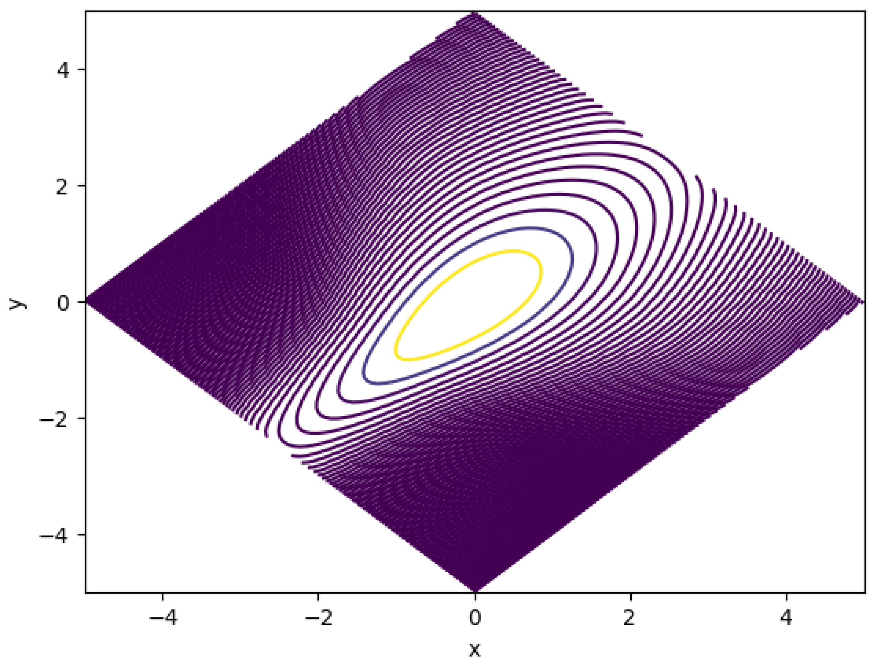
We show one example of 2-d case: We discretize p and f together and solve for p first for a time step, and then solve for f. We don’t use chain rule to break out the partial derivatives of product but instead discretize on the product. With standard finite difference methods, the calculation is fast and stable. We present an example of the distribution below:

Figure 1 shows the contour of a Gaussian distribution with correlation skew. The underlying correlation function is:

$$\rho (u)=\left\{\begin{array}{cc}0.9\hfill & \mathrm{if}u<-2\sqrt{t}\hfill \\ 0.9-{\displaystyle \frac{u+2\sqrt{t}}{4\sqrt{t}}}0.4\hfill & \mathrm{if}-2\sqrt{t}\le u<2\sqrt{t}\hfill \\ 0.5\hfill & \mathrm{if}u\ge 2\sqrt{t}\hfill \end{array}\right.$$

The graph axis is in x and y. Note $u,v$ will be the two diagonal directions.

The shape of the contour is expected. As we put higher correltion when the $u={\displaystyle \frac{x+y}{2}}$ is lower, and lower correlation when u is higher, the probability is more concentrated when u is low and more dispersed when u is high. Note with u fixed, the graph also shows symmetry in the direction of v.

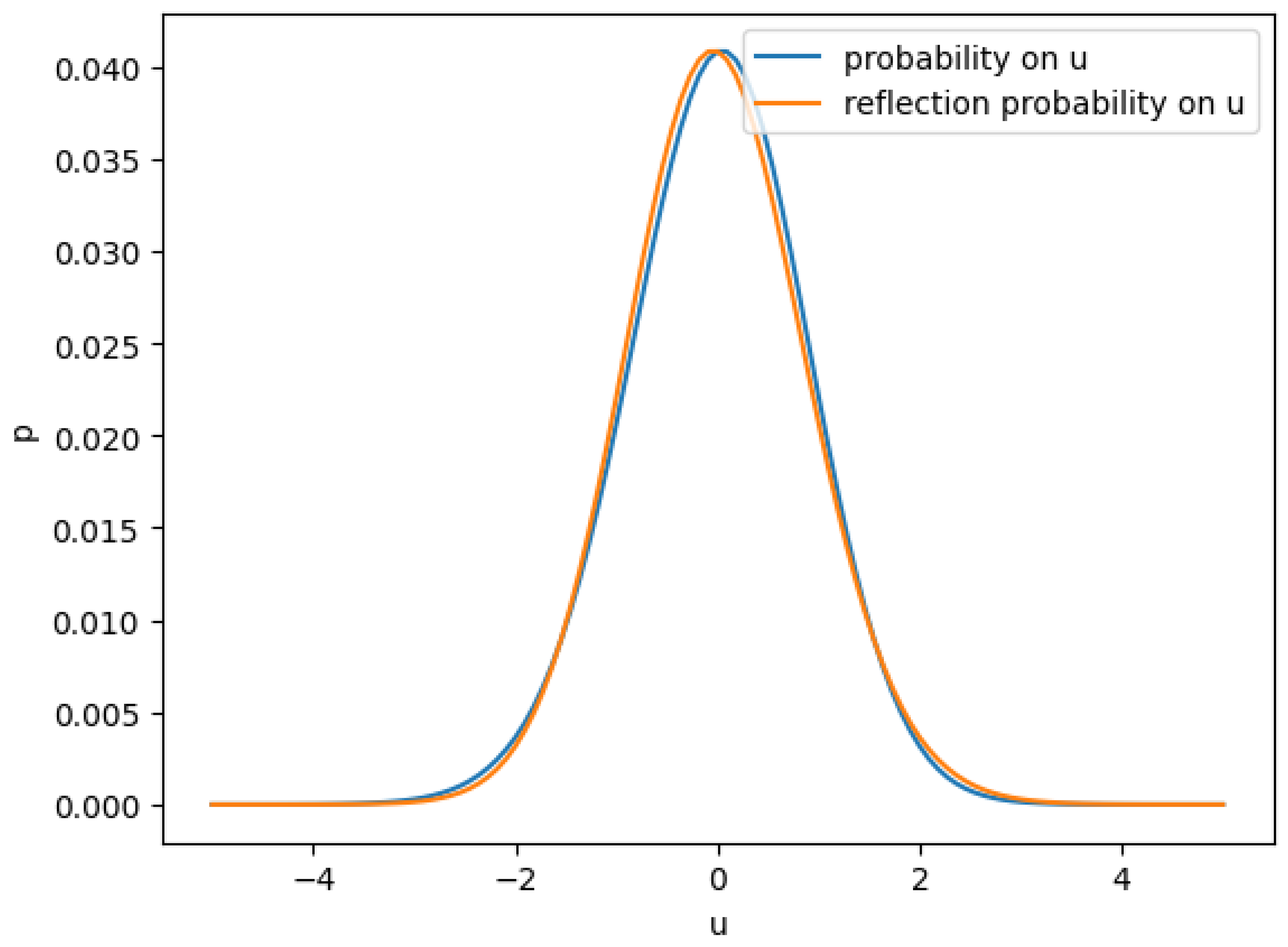
The following graphs shows more details on $p(u)$ in above example.

In Figure 2 the distribution of u is very close but different to a standard normal. To see the difference, we reflected the probability around center and then one can see the negative part has a fatter tail than positive part.

This is expected as we correlated $x,y$ more when $x+y$ is more negative, we expect $x+y$ will have more potential to go lower in the negative direction, and as we de-correlate $x,y$ more when $x+y$ more positive, we expect the diversifying effect makes the $x+y$ less potential to go higher when $x+y$ positive.

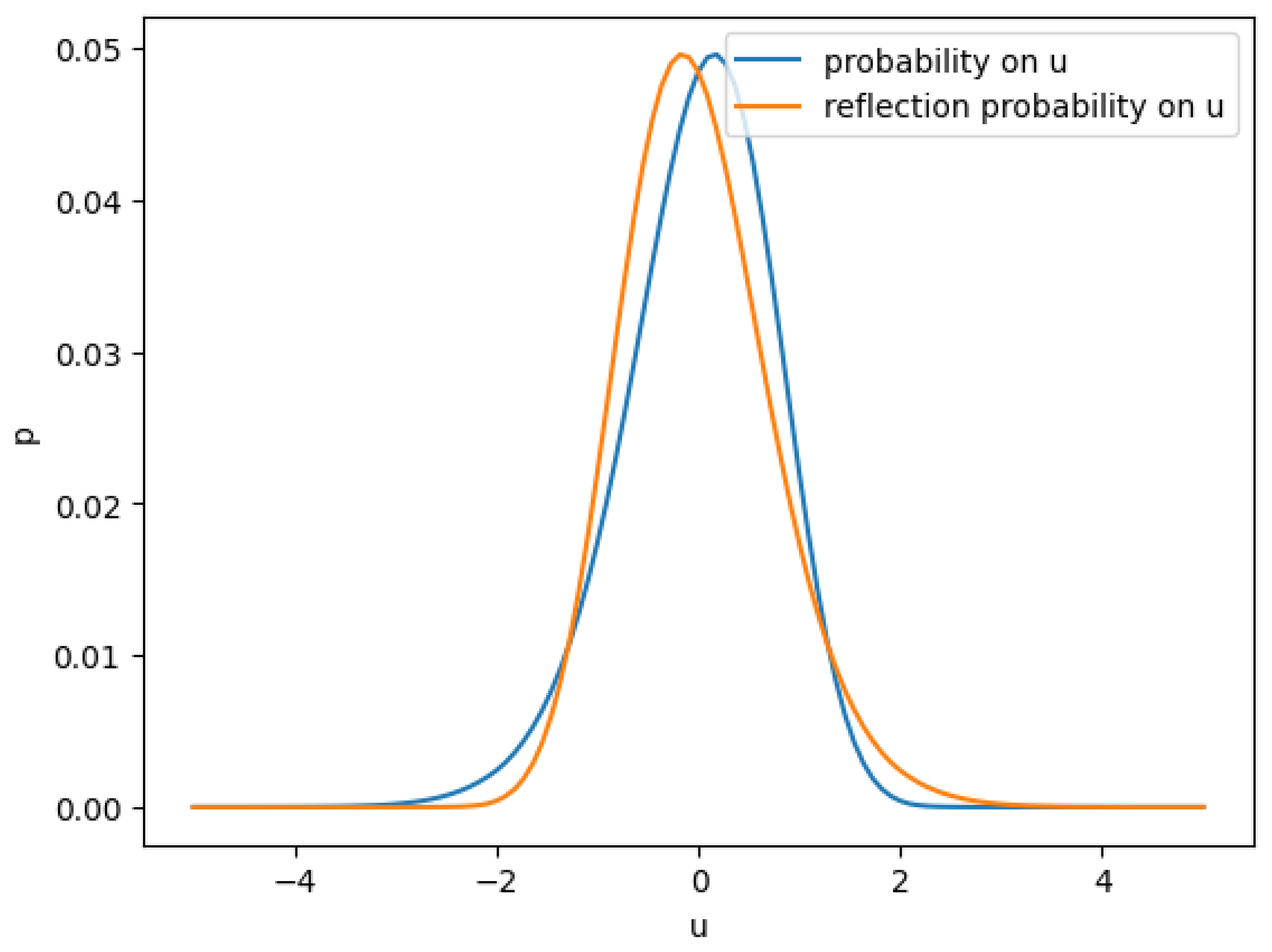
To demonstrate this point, we can increase the skew of correlation further to see the fat tail effect. Below is the $p(u)$ for a more skewed correlation function.

The correlation function in Figure 3 is

$$\rho (u)=\left\{\begin{array}{cc}0.9\hfill & \mathrm{if}u<-2\sqrt{t}\hfill \\ 0.9-{\displaystyle \frac{u+2\sqrt{t}}{4\sqrt{t}}}1.4\hfill & \mathrm{if}-2\sqrt{t}\le u<2\sqrt{t}\hfill \\ -0.5\hfill & \mathrm{if}u\ge 2\sqrt{t}\hfill \end{array}\right.$$

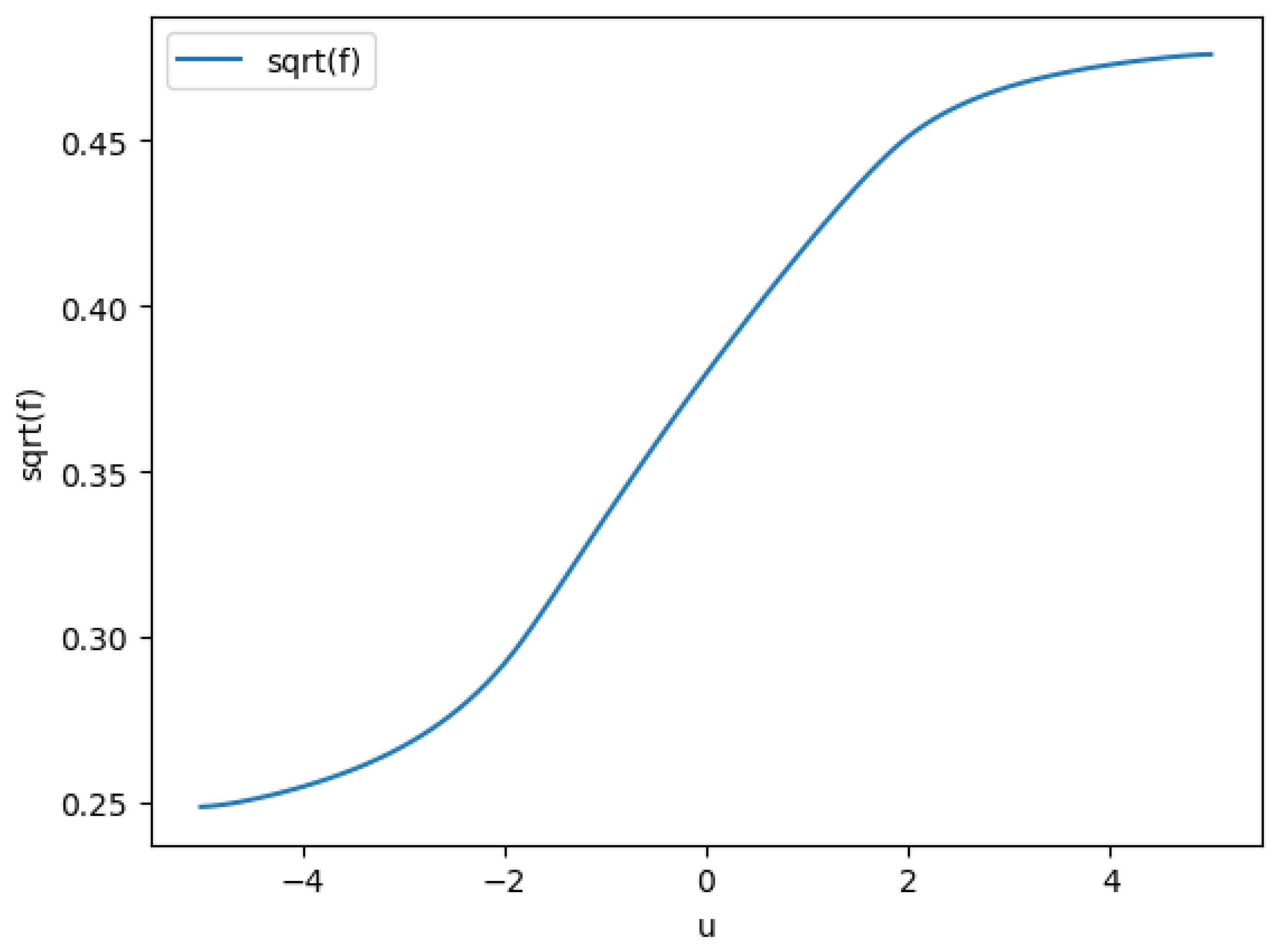
The coutour in Figure 1 shows the v is concentrated when u more negative and v is spreaded when u is more positive. Below Figure 4 shows the std dev of v conditioned on u, ie, the $\sqrt{f}$ function.

5. Copula Application

Knowing the $p(u)$ and $f(u)$ we can integrate any function on this approximated terminal distribution. For given $u,v$, it maps to $x,y$, and the marginal distribution of x and y are approximated normal distribution respectively (Note that the true terminal distribution will have the marginals as true normal distribution, as we approximate the terminal we can think we approximated the marginals), so they can be readily used to invert CDFs.

We found the moment matching to 2nd order produces good accuracy in our tests.

References

- Fokker, A. D. (1914). Die mittlere energie rotierender elektrischer dipole im strahlungsfeld. Annalen der Physik, 348(5), 810–820. [CrossRef]
- Kolmogorov, A. (1931). ¨Uber die analytischen methoden in der wahrscheinlichkeitstheorie. Math Annal, 104, 415–458. [CrossRef]
- Lucic, V. (2012). Correlation skew via product copula. In Financial engineering workshop, cass business school.
- Luján, I. (2022). Pricing the correlation skew with normal mean–variance mixture copulas. Journal of Computational Finance, 26(2).
- Planck, V. (1917). ¨Uber einen satz der statistischen dynamik und seine erweiterung in der quantentheorie. Sitzungberichte der.