
Submitted:
08 January 2025
Posted:
09 January 2025
You are already at the latest version
Abstract
In this paper a new algorithm for the training of Locally Recurrent Neural Networks (LRNNs) is presented, which aims to reduce computational complexity and at the same time to guarantee the stability of the network during the training. The main feature of the proposed algorithm is the capability to represent the gradient of the error in an explicit form. The algorithm builds on the interpretation of the Fibonacci’s sequence as the output of an IIR second-order filter, which makes it possible to use the Binet’s formula that allows the generic terms of the sequence to be calculated directly. Thanks to this approach, the gradient of the loss function during the training can be explicitly calculated, and it can be expressed in terms of the parameters, which control the stability of the neural network.
Keywords:
1. Introduction
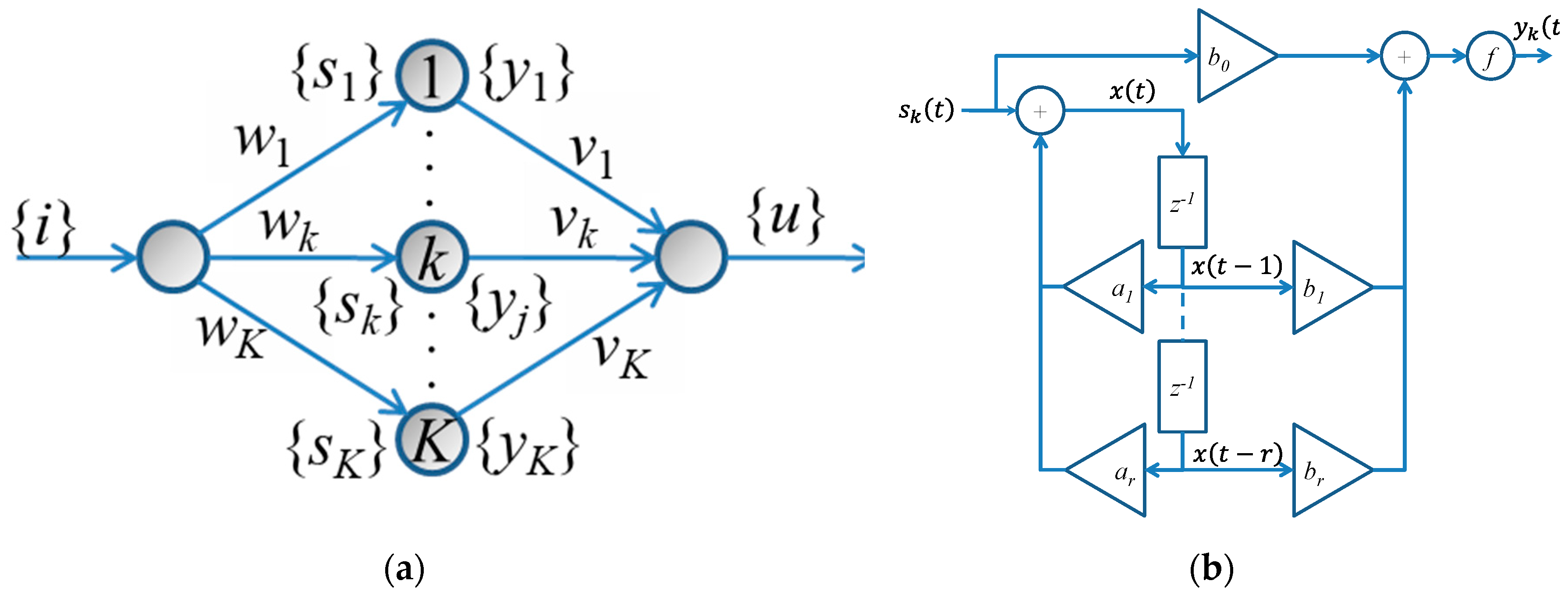
2. Neural Model
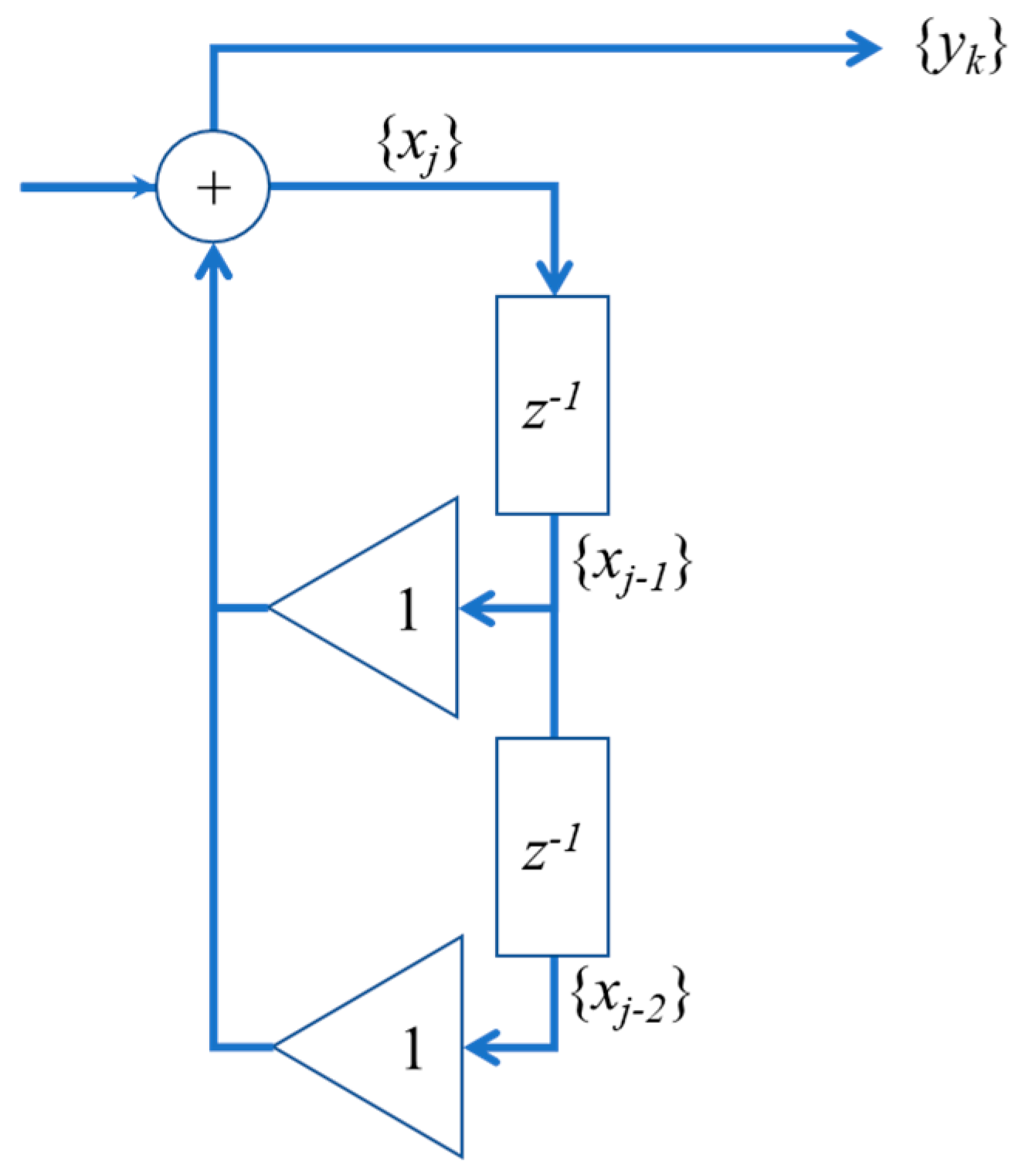
2.1. The Fibonacci’s Series and the Binet’s Formula
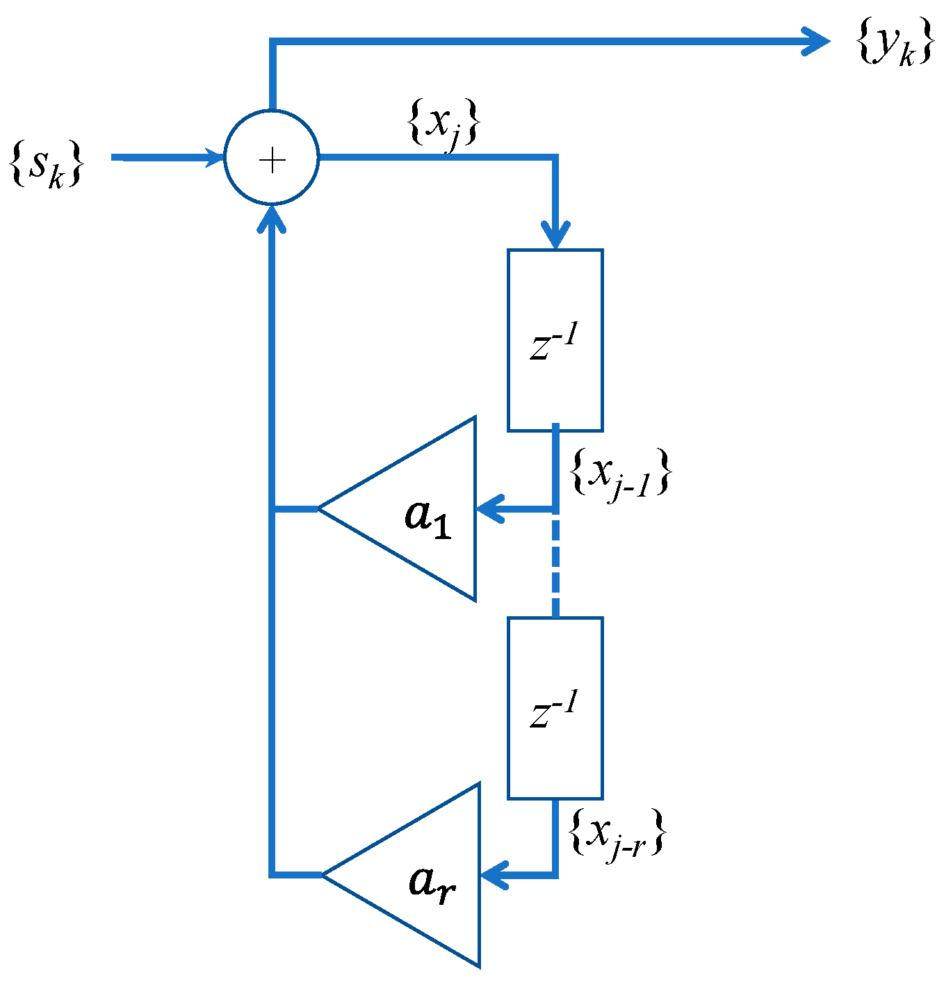
2.2. Exploitation of the Binet’s Formula to Calculate the IIR Impulsive Response
2.3. Derivative of the Loss Function with Respect to the Feedback Parameters
2.4. The Training Algorithm
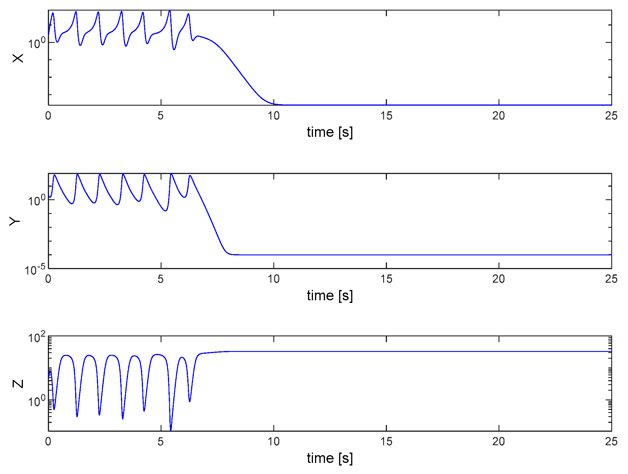
3. Results
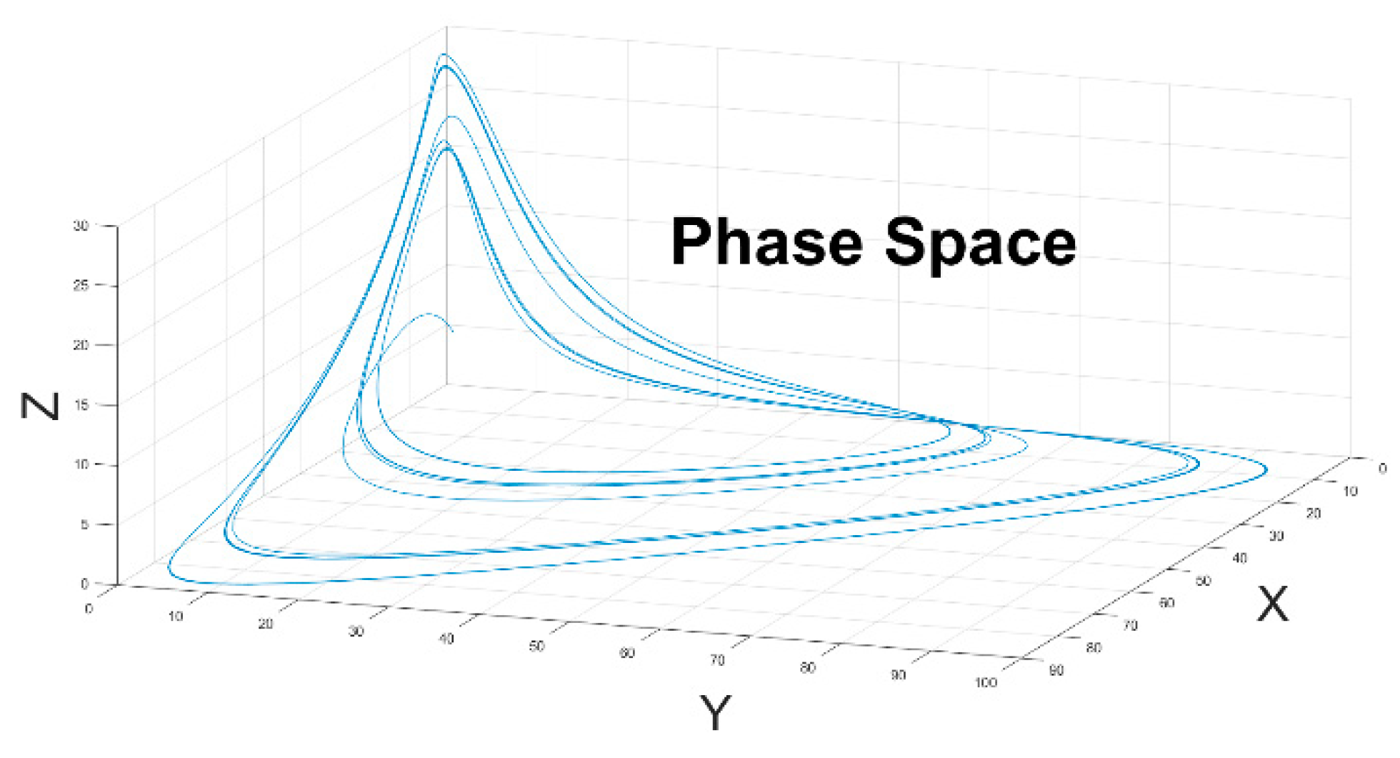
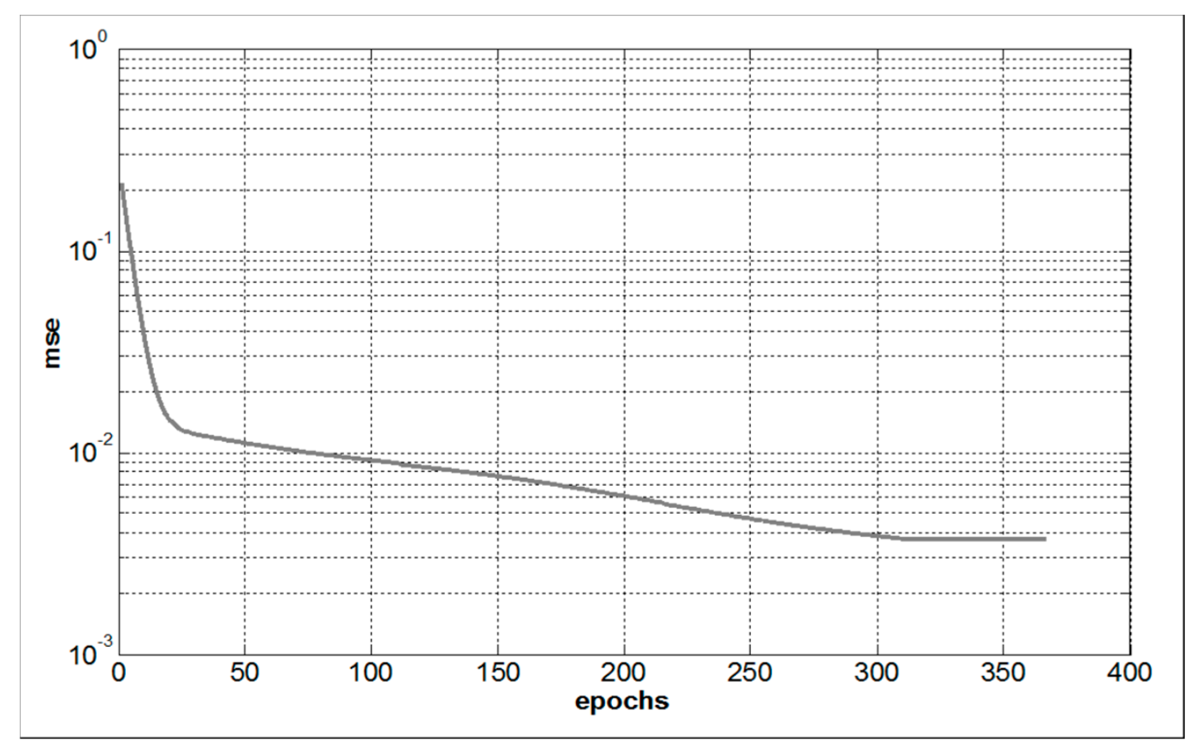
4. Discussion and Conclusion
Author Contributions
References
- Han, Y.; Huang, G.; Song, S.; Yang, L.; Wang, H.; Wang, Y. Dynamic Neural Networks: A Survey. IEEE Transactions on Pattern Analysis and Machine Intelligence 2022, 44, 7436–7456. [Google Scholar] [CrossRef] [PubMed]
- Waibel, A. Modular Construction of Time-Delay Neural Networks for Speech Recognition. Neural computation 1989, 1, 39–46. [Google Scholar] [CrossRef]
- Bromley, J.; Guyon, I.; LeCun, Y.; Säckinger, E.; Shah, R. Signature Verification using a “Siamese” Time Delay Neural Network. In Proceedings of the Advances in Neural Information Processing Systems; Morgan-Kaufmann, 1993; Vol. 6.
- Cao, J.; Wang, J. Global asymptotic and robust stability of recurrent neural networks with time delays. IEEE Transactions on Circuits and Systems I: Regular Papers 2005, 52, 417–426. [Google Scholar] [CrossRef]
- Huang, W.; Yan, C.; Wang, J.; Wang, W. A time-delay neural network for solving time-dependent shortest path problem. Neural Networks 2017, 90, 21–28. [Google Scholar] [CrossRef] [PubMed]
- Nerrand, O.; Roussel-Ragot, P.; Personnaz, L.; Dreyfus, G.; Marcos, S. Neural Networks and Nonlinear Adaptive Filtering: Unifying Concepts and New Algorithms. Neural Computation 1993, 5, 165–199. [Google Scholar] [CrossRef]
- Htike, K.K.; Khalifa, O.O. Rainfall forecasting models using focused time-delay neural networks. In Proceedings of the International Conference on Computer and Communication Engineering (ICCCE’10); 2010; pp. 1–6.
- Grossberg, S. Nonlinear neural networks: Principles, mechanisms, and architectures. Neural Networks 1988, 1, 17–61. [Google Scholar] [CrossRef]
- Haykin, S.S. Adaptive Filter Theory; Pearson Education, 2002; ISBN 978-81-317-0869-9.
- Widrow, B.; Glover, J.R.; McCool, J.M.; Kaunitz, J.; Williams, C.S.; Hearn, R.H.; Zeidler, J.R.; Eugene Dong, Jr.; Goodlin, R.C. Adaptive noise cancelling: Principles and applications. Proceedings of the IEEE 1975, 63, 1692–1716. [Google Scholar] [CrossRef]
- Pedro, J.C.; Maas, S.A. A comparative overview of microwave and wireless power-amplifier behavioral modeling approaches. IEEE Transactions on Microwave Theory and Techniques 2005, 53, 1150–1163. [Google Scholar] [CrossRef]
- Krotov, D. A new frontier for Hopfield networks. Nat Rev Phys 2023, 5, 366–367. [Google Scholar] [CrossRef]
- Jordan, M.I. Chapter 25 - Serial Order: A Parallel Distributed Processing Approach. In Advances in Psychology; Donahoe, J.W., Packard Dorsel, V., Eds.; Neural-Network Models of Cognition; North-Holland, 1997; Vol. 121, pp. 471–495.
- Elman, J.L. Finding Structure in Time. Cognitive Science 1990, 14, 179–211. [Google Scholar] [CrossRef]
- Back, A.D.; Tsoi, A.C. FIR and IIR Synapses, a New Neural Network Architecture for Time Series Modeling. Neural Computation 1991, 3, 375–385. [Google Scholar] [CrossRef] [PubMed]
- Tsoi, A.C. Recurrent neural network architectures: An overview. In Adaptive Processing of Sequences and Data Structures: International Summer School on Neural Networks “E.R. Caianiello” Vietri sul Mare, Salerno, Italy September 6–13, 1997 Tutorial Lectures; Giles, C.L., Gori, M., Eds.; Springer: Berlin, Heidelberg, 1998; ISBN 978-3-540-69752-7. [Google Scholar]
- Campolucci, P.; Piazza, F. Intrinsic stability-control method for recursive filters and neural networks. IEEE Transactions on Circuits and Systems II: Analog and Digital Signal Processing 2000, 47, 797–802. [Google Scholar] [CrossRef]
- Werbos, P.J. Backpropagation through time: what it does and how to do it. Proceedings of the IEEE 1990, 78, 1550–1560. [Google Scholar] [CrossRef]
- Campolucci, P.; Uncini, A.; Piazza, F. Causal back propagation through time for locally recurrent neural networks. In Proceedings of the 1996 IEEE International Symposium on Circuits and Systems. Circuits and Systems Connecting the World. ISCAS 96; 1996; Vol. 3, pp. 531–534 vol.3.
- Campolucci, P.; Uncini, A.; Piazza, F. Fast adaptive IIR-MLP neural networks for signal processing applications. In Proceedings of the 1996 IEEE International Conference on Acoustics, Speech, and Signal Processing Conference Proceedings; 1996; Vol. 6, pp. 3529–3532 vol. 6.
- Campolucci, P.; Piazza, F. Intrinsic stability-control method for recursive filters and neural networks. IEEE Transactions on Circuits and Systems II: Analog and Digital Signal Processing 2000, 47, 797–802. [Google Scholar] [CrossRef]
- Battiti, R. First- and Second-Order Methods for Learning: Between Steepest Descent and Newton’s Method. Neural Computation 1992, 4, 141–166. [Google Scholar] [CrossRef]
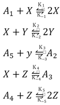
- Willamowski, K.-D.; Rössler, O.E. Irregular Oscillations in a Realistic Abstract Quadratic Mass Action System. Zeitschrift für Naturforschung A 1980, 35, 317–318. [Google Scholar] [CrossRef]
- Niu, H.; Wang, H.; Zhang, Q. The Chaos Anti-control in the Willamowski-Rössler Reaction. In Proceedings of the 2010 International Workshop on Chaos-Fractal Theories and Applications; 2010; pp. 87–91.
Disclaimer/Publisher’s Note: The statements, opinions and data contained in all publications are solely those of the individual author(s) and contributor(s) and not of MDPI and/or the editor(s). MDPI and/or the editor(s) disclaim responsibility for any injury to people or property resulting from any ideas, methods, instructions or products referred to in the content. |
© 2025 by the authors. Licensee MDPI, Basel, Switzerland. This article is an open access article distributed under the terms and conditions of the Creative Commons Attribution (CC BY) license (http://creativecommons.org/licenses/by/4.0/).


