
Submitted:
04 January 2025
Posted:
08 January 2025
You are already at the latest version
Abstract
This paper introduces a mixed causal-noncausal invertible-noninvertible autoregressive moving average generalized autoregressive conditional heteroskedasticity (MARMA-GARCH) model, which uniquely combines features to capture the nonlinear dynamics observed in financial markets. The MARMA component replicates explosive episodes observed during financial bubbles, while the GARCH model effectively captures time-varying conditional volatility. We propose two methods for parameter estimation: the Whittle function in the frequency domain and the maximum likelihood. Additionally, we suggest an identification scheme through high-order spectral densities and high-order dynamics of the residuals. Our findings demonstrate that an incorrect identification of the MARMA process leads to biased GARCH parameters, underestimating the effect of news and overestimating the volatility clustering. An empirical application to Bitcoin and Ethereum reveals the existence of noncausal dynamics in the mean, jointly with significant GARCH effects.
Keywords:
ARMA
; noncausal
; noninvertible
; financial bubbles
; GARCH
; spectral density
; Cryptocurrency
1. Introduction
Financial returns often exhibit weak autocorrelation but strong and persistent volatility, posing challenges for traditional models to achieve independent errors. The mixed causal-noncausal invertible-noninvertible autoregressive moving average (MARMA) model emerges as a generalization of the ARMA model, allowing the autoregressive and moving average polynomials to have roots outside but also inside the unit disk. Whereas the non-invertible process is well known, a more recent literature studies the presence of a non-causal component that can generate local explosions commonly observed in financial asset prices, motivating their use in economic applications.1
A key feature, and one of the most challenging aspects, of a MARMA process is that it admits multiple ARMA representations, each sharing the same second-order probability structure. This is advantageous for estimation, as all representations possess an identical variance-covariance matrix and, thus, the same spectral density. However, this multiplicity poses a challenge for identification. Roots inside and outside the unit disk result in the same values of the estimation function under Gaussian estimation methods like least squares, Yule-Walker, or maximum likelihood. This is the case with the most common ARMA representation of the MARMA process, which assumes that the roots are outside the unit disk, known as the causal and invertible ARMA representation [12]. Identification becomes feasible when the assumption of normality is relaxed, each representation having a unique and identifiable higher-order probability structure. These differences are evident in the autocorrelation functions of the squared residuals and the higher-order spectral densities, revealing significant dynamics.
The MARMA model can generate nonlinear dynamics similar to those produced by the Generalized Autoregressive Conditional Heteroskedasticity (GARCH) model [8]. However, the MARMA model has a distinct probability structure, incorporating second-, third-, and fourth-order relationships. [39] show that the nonlinear dynamics inherent in the MARMA model differ significantly from those of the GARCH model due to the involvement of third and fourth-order cumulants and the interactions between errors and future values of the time series. Furthermore, [12] noted that although all-pass models can produce nonlinear dynamics, their high-order probability structure is not sufficient to compete with the GARCH model, as they cannot replicate the well-known clustering effect, where small variations are followed by small variations and large variations are followed by large variations [22].
This limitation is particularly evident in financial returns that exhibit weak autocorrelation but extreme and persistent volatility, where no MARMA model can achieve independent errors. Conversely, the squared errors display significant dynamics, as seen in the log-returns of major cryptocurrencies [51], stocks, commodities, and market indexes [16]. To replicate this characteristic, it becomes a natural option to relax the assumption of i.i.d. errors and to introduce a more flexible form that allows for time-varying volatility. This approach implies adding a GARCH process to the errors. Such models could provide a better fit for financial returns, especially during periods of high volatility and extreme values, as observed during recent financial crises.
This new approach presents challenges in estimation and identification, as it departs from the traditional assumption of i.i.d. errors in the MARMA model. While the theory surrounding the estimation of the MARMA model typically assumes that the sequence of errors follows an i.i.d. process, [47] consider maximum likelihood estimation of non-invertible ARMA models with ARCH errors, providing conditions under which a strongly consistent and asymptotically normal distributed solution to the likelihood equations exists under a finite variance. We generalize [47] to the estimation and identification of the MARMA-GARCH model, which can be not only noninvertible but also noncausal. We investigate the use of the Whittle estimation in the frequency domain as well as the maximum likelihood. In both methods we first estimate the MARMA model and compute the error process on which we estimate the GARCH parameters. This thorough comparison is valuable because both methods are equivalent in estimating the MARMA process, sharing similar characteristics of consistency and asymptotic normality. For example, both require a stationary environment and finite variance, and they perform well with heavy-tailed errors. However, for the GARCH processes, maximum likelihood estimation only requires the existence of the variance of the process, while the Whittle estimation requires the existence of eight moments, representing a limitation for financial returns that often exhibit extreme tails. Therefore, we compare the performance of Whittle and maximum likelihood estimation methods, providing a comprehensive understanding of their strengths and limitations. Our Monte Carlo study reveals that the MLE produces parameter estimates with lower bias and less standard deviation.
The paper is organized as follows: In Section 2, we present the MARMA-GARCH model along with the methods for estimation and identification and the techniques for detrending the data. Section 3 provide the results of the Monte Carlo simulations, and the empirical application to cryptocurrencies. Finally, we conclude with a discussion and conclusion in Section 4.
2. Materials and Methods
2.1. MARMA()-GARCH() Processes
Let be a univariate mixed causal-noncausal invertible-noninvertible autoregressive moving-average generalized autoregressive conditional heteroskedasticity MARMA ()-GARCH() process that is stationary for every , and represented by:
The sequence of innovations is assumed to be i.i.d. with zero mean and unit variance, and is a probability density function with as its parameters.
where the sequence is a martingale difference with moments and cumulants:
Let denotes the backward shift operator for . The lag polynomials and , and the lead polynomials and are defined as:
We define the MARMA() parameter vector as
Note that for and , the MARMA() model becomes the causal and invertible ARMA() model, under the assumption that the dependency structure is exclusively determined by lagged terms. On the other hand, the GARCH polynomials are defined as:
For , , , also , and ensures the non-negativity of the GARCH process . The parameter vector of the GARCH() is defined as
Equation 1 can be expanded as follows:
We assume that all common roots between and are canceled. Moreover, the polynomials , , and have their zeros outside the unit disk. For the GARCH polynomials, we assume no common roots and roots strictly outside the unit disk. The polynomials can be expressed in terms of their roots:
Note that the MARMA inverse polynomials admit individual Laurent expansions. Consequently, the MARMA() model admits a two-sided representation, an MA(∞), and an AR(∞) as discussed in p. 88 [14]. The MA(∞) representation is given by:
where are the coefficients of in the Laurent expansion of . Note that is absolutely convergent in the annulus . Therefore, are the zeros of the polynomials and . Similarly, are the zeros of the polynomials and . The polynomials can be factorized as follows:
Note that in Equations (16-), any root z can be replaced by its inverse without altering the second-order moments of the MARMA process. Indeed, there exist possible MARMA models to represent the process. Each model can produce uncorrelated but not independent errors in the finite variance setting since they share the same second-order moments. Consequently, the MARMA() and the ARMA() processes have the same ACF and second-order spectral density. As a result, the two processes are not identifiable under the assumption of Gaussianity. On the contrary, under a non-Gaussian distribution, each process has a different and identifiable probability structure that relies on the high-order moments.
According to [22], a squared GARCH() model can be reformulated as an ARMA() model. Thus, Equation (3) can be rewritten as:
where . We assume that is strictly stationary, with , therefore, are martingale differences. The RHS of Equation 20 can be factorized in terms of the polynomials:
and
We can observe that, as in Equation 16, the roots of the polynomials of the GARCH process can also lie outside the unit disk without altering the second-order probability structure of the model. As a consequence, the squared errors () can be expressed as an ARMA() with martingale differences ():
The equivalence between Equations (3) and (20) was proposed by Bollerslev (1986). This equivalence allows us to estimate the parameters in Equation (23) using the properties of , which is uncorrelated but not independent. In this context, the parameters of the GARCH model can be estimated using standard procedures such as Gaussian maximum likelihood and least squares. However, it is important to note that is uncorrelated but not independent and identically distributed (i.i.d.) since it depends on the past values of . Therefore, this representation is called the squared of a GARCH process.
2.1.1. Causal and Invertible Representation
A MARMA() process can be represented in multiple ARMA() forms, where and , all maintaining the same second-order dependency structure [39]. One such form is the causal and invertible representation,2 characterized by polynomial roots outside the unit disk. For noncausal and noninvertible data-generating processes, this representation yields errors that are uncorrelated but not independent ([12]). However, estimating the invertible all-pass model allows for identifying the roots of the noncausal and noninvertible polynomials through the factorization in Equation 16. The causal and invertible representation is described by:
with being uncorrelated but not independent, and where and are polynomials of order p and q, respectively, and only depending on lagged terms. Therefore, Equation 10 can be expressed as:
Considering that the coefficients and are invariant to the allocation of the roots, we establish , and . The causal and invertible representation of the MARMA() process is:
The set of parameters is . The representation is causal since there exists a sequence of constants , such that , with and expressed in terms of the present and past of the error sequence, which is an MA(∞). On the other hand, it is invertible since there exists a sequence of constants , such that , with . Hence, is formulated in terms of both the present and historical values of , characterizing an AR(∞) process.
The causal and invertible representation is typically obtained using traditional estimation methods. However, there is a risk that misspecification of the roots may lead to residuals that are uncorrelated but not independent, especially showing dynamics in the squared residuals that differ from those of the GARCH process (see [39], for details). This is why we expect that the errors arising from the MARMA process and its causal and invertible representation will differ regarding the GARCH estimated parameters and the higher-order dynamics.
2.1.2. Spectral Representations
The spectral representation of the model is divided into two parts: the MARMA part and the GARCH part. The spectral density of the MARMA model was proposed by [39], where it is shown to be equivalent to that of the MARMA() model in second-order moments. The spectral density of the GARCH part is generated through its ARMA() representation with conditionally heteroskedastic innovations proposed by [8].
Let be a MARMA()-GARCH() process satisfying Equation 1. The transfer function for the conditional mean is:
The k-th order spectral density is given by:
where is the k-th order cumulant, are the Fourier frequencies for , where T is the length of the data, and is a root represented by a complex number. Following Equation 27, the second-order (), third-order (), and fourth-order () spectral densities are:
On the other hand, the transfer function for the conditional variance is defined as:
The k-th order spectral density is given by:
where is the k-th order cumulant of (). In the same reasoning as in the MARMA part, the spectral densities for are:
The k-th order periodogram gives the sample counterpart of the k-th order spectral density:
where is the discrete Fourier transform. For , Equation 36 is the periodogram, for is the biperiodogram, and for is the triperiodogram:
where and are the complex conjugates of the Fourier transform evaluated at the sum of two and three frequencies, respectively.
2.2. Parameter Estimation and Identification
We propose a two-step estimation procedure. First, we estimate the parameters of the MARMA() model using the causal and invertible ARMA() representation. We select the order p and q based on information criteria (BIC and AIC) and the significance of coefficients, preferring the most parsimonious form. Then, we factorize the AR and MA polynomials to explore all combinations of roots that result in noncausal and noninvertible models. To select the best-fitting model, we choose the one that produces residuals with the least high-order dependence. We use a high-order spectral function proposed by [50] and a Portmanteau-type test on the residuals and squared residuals.
In the second step, we estimate the GARCH() model, again using information criteria to select p and q. However, it is commonly known that GARCH(1,1) often adequately represents the conditional volatility dynamics in financial assets. We compare the Whittle and time-domain maximum likelihood estimations to determine which method better captures the high-order dynamics.
2.2.1. Estimation and Identification of the MARMA() Process
We consider the Whittle estimation of the causal and invertible ARMA() model based on the observations of the MARMA() process. Minimizing the Whittle estimator is asymptotically equivalent to the Gaussian-likelihood given that the distribution of the Fourier transforms of converges in distribution to independent complex normal variables. Therefore, the periodogram tends in probability to the second-order spectral density.
The causal and invertible representation satisfies the usual Yule-Walker equations as the ACF of its residuals converges to the ACF of the MARMA() model, also as they have identical second-order spectral density. Consequently, it can be consistently estimated using the Whittle function; see [25] for a detailed overview. The Whittle estimator of is:
The estimated parameter set is obtained by minimizing the function:
Once obtained the set of estimated parameters of the causal and invertible ARMA() representation, we proceed to construct all possible representations, restricted to the order and . For this purpose, we factorize the polynomials and . Second, we distribute all the roots using Equation 16, to construct polynomials and .
The global minimum is achieved if , and . [35] demonstrated that the Whittle estimator is consistent: , as . The asymptotic distribution of the estimator is Gaussian: . On the other hand, the asymptotic variance-covariance matrix of the estimator can be approximated by the inverse of the Fisher information matrix: . The Fisher information criteria are computed in the frequency domain:
Notice that the Whittle estimator convergence to its true value occurs when , which ensures that the periodogram converges to the second-order spectral density ([49]). In a context of infinite variance, the mean of the periodogram cannot converge to the spectral density, leading to biased parameters and invalid inference.
The Hessian matrix is defined as the second-order partial derivatives of the Whittle function with respect to the parameter vector :
2.2.2. Spectral Identification Function
[50] propose to combine the third- and fourth-order spectral densities into a single function, which captures the information about the respective order dynamics. These dynamics align with those observed in the residuals of a misspecified model, as illustrated in [39] Example 1. The combined spectral function is:
where . The denominator represents the k-th order transfer function, evaluated using the causal and invertible model parameters. When high-order dynamics are absent, the discrepancy between the k-th order periodogram and the spectral density follows a multivariate normal distribution:
For and , the spectral identification function is:
2.2.3. Portmanteau-Type i.i.d. Test
We use the Portmanteau-type test proposed by [42]; however, we employ a simplified version that only considers the autocorrelation of the residuals and the squared residuals.3 Under these conditions, the test converges to the one proposed by [19], which combines the autocorrelation function (ACF) of the errors, , and the squared errors, , into a single function. The premise is that if is i.i.d., then . The test includes both individual lag and cumulative versions:
The null hypothesis for the individual lag is for , and for the cumulative test, for , where m is the number of lags. The asymptotic distributions of the tests are given by:
These tests effectively detect dependence, conditional heteroscedasticity, or nonstationarity. The distribution is a suitable approximation for the asymptotic distribution of the test for non-Gaussian processes. The identification of the MARMA process is determined by the model for which the null hypothesis is not rejected. If the null hypothesis is rejected for two models, the model with the smallest value of the statistic is selected.
The spectral function integrates third- and fourth-order spectral density functions, effectively identifying the correct MARMA model when the error distribution exhibits skewness or kurtosis. Conversely, the test by [19] utilizes information from the ACF of the residuals and the squared residuals in a cumulative function, enabling the identification of the correct model based on the minimum value of the function evaluated across all possible representations. The performance of both functions in identifying MARMA is proposed in [39]. Under non-Gaussianity, both methods are reliable for identification. However, the function by [50] yields better results for asymmetric distributions.
2.2.4. Whittle Estimation for the GARCH()
Whittle estimation for the GARCH() model was initially proposed by [27], using the ARMA(max(),q) representation as suggested in Equation 23. Although this relationship indicates that Whittle estimation can be used for parameter estimation of the GARCH model, the assumptions on the moments of are more stringent; specifically, , which is quite restrictive. This is in contrast with empirical evidence on financial returns, which sometimes exhibit infinite second, third, or fourth moments. Later, [48] demonstrated that Whittle estimation for the squared GARCH process is feasible with only the existence of the fourth moment of . However, the convergence of the estimated parameters is significantly slower compared to the time-domain maximum likelihood estimation.
The Whittle estimator of is:
The estimated parameter set is obtained by minimizing the function:
Unlike the maximum likelihood, the Whittle estimator relies solely on the values . This means that the unobservable values do not need to be evaluated, and there is no need to choose initial values for . This characteristic can be seen as an advantage of the Whittle estimator. The parameter is estimated by the unconditional variance, :
The question arises regarding the potential use of Whittle estimation for the GARCH model in the context of noncausality or noninvertibility of the mean model. Although its implementation can be straightforward, there are gaps concerning its validity, given that the mean and volatility models are separated. While the mean can depend on future values, the volatility, in this case, only depends on past shocks.
2.2.5. Maximum Likelihood Estimation for the GARCH()
The most common estimation method for the GARCH model is through the maximum likelihood function, as it is consistent and asymptotically normal for stationary GARCH processes [24]. In contrast to the Whittle estimator, which requires the existence of the fourth moments of for GARCH models, the maximum likelihood function does not make assumptions about the moments. Given that we do not make assumptions about the distribution of the innovations , but we use the likelihood function of the normal distribution, this estimator is usually referred to as quasi-maximum likelihood.
Given the parameter vector of the GARCH(): , the likelihood function is conditioned to the initial values , and can be defined by:
where is as in Equation 3, and recursively generated for , . The log-likelihood function is defined as:
The minimization obtains the estimation of the parameters:
The estimator is consistent, , given that converges in probability to the true parameter set as . The true parameter is identifiable if the likelihood function has a unique minimum at . This identifiability condition ensures that no other parameter vector can produce the same likelihood as the true parameter vector. Furthermore, the estimation function converges uniformly to its expectation. Specifically, the log-likelihood function converges in probability to its expected value as T grows. This is expressed as for all . The uniform convergence implies that for any small and , there exists a sample size such that for all , the probability that the supremum of the absolute difference between the normalized log-likelihood function and its expectation is less than exceeds . Therefore, the convergence of the log-likelihood function to its expectation does not depend on the specific parameter value but holds uniformly over the entire parameter space .
The estimator is asymptotically normal as . This is expressed as , where is the Fisher information matrix evaluated at the true parameter values. The Fisher information matrix is defined as:
where is the conditional density of given past information . The score function, defined as , satisfies the Central Limit Theorem; therefore, the score vector evaluated at the true parameter values has an asymptotically normal distribution. Additionally, the Hessian matrix of the log-likelihood function, normalized by T, must converge in probability to the Fisher information matrix. Formally, . Consequently, the distribution of the estimator is approximately normal, centered at the true parameter values, and with a covariance matrix given by the inverse of the Fisher information matrix.
The assumptions regarding the moments of the process are as follows. First, the variance of the process must be finite, , to ensure the model parameters are estimable. Additionally, the existence of fourth-order moments, , is necessary to derive the asymptotic properties of the estimators, ensuring that the sample moments converge to their population counterparts. Specifically, the Fisher information matrix, , must be finite and positive definite to ensure that the parameter estimates have a well-defined asymptotic distribution and that the covariance matrix of the estimators is invertible.
These assumptions hold under the condition that is strictly stationary. However, financial asset prices typically exhibit trends and are not stationary. Therefore, we propose techniques for detrending in the following sections.
2.3. Detrending Method
Removing the trend from data is a topic of considerable debate since the choice of method can directly influence the emergence of dynamics. For instance, the econometrician must make assumptions about the nature of the trend, whether it is stochastic or deterministic. To address this, the econometrician may utilize tests such as the augmented Dickey-Fuller or Phillips-Perron tests. However, the outcomes of these tests depend on the choice of lag length, and the empirical distribution of the test may not align with the data generating process, potentially leading to inference errors.
When selecting a stochastic trend, the most common method is to differentiate the data, though the optimal number of differences needs to be well-established. Another approach could be a logarithmic transformation. In both cases, the primary concern is that incorrect differencing or transformation can remove or add relevant information about the time series dynamics, leading to the emergence of spurious dynamics.
In the case of choosing a deterministic trend, the econometrician must determine the optimal number of polynomials to fit the trend. Practically, this is done through visual inspection and information criteria, although there is no clear rule for this choice, which can result in either the appearance of spurious dynamics or the abstraction of significant dynamics. Various methods have been proposed in the literature. For instance, [41] employed a cubic trend, while [25] and [1] utilized a linear trend or simple centering. [18] used returns, whereas [37] applied the X-11 method to filter seasonal effects. Another method is the Hodrick-Prescott filter, which has been used by [40] and shows that for monthly data, the filter may not induce dynamics. However, in practice, the selection of the lambda parameter influences the dynamics obtained in the time series; see [34] for details. Recently, a filtering approach was proposed by [5], based on a joint model that includes both a random-walk fundamental component and a bubble component specified as a MAR model. Both components are treated simultaneously in the filter updating process, allowing the test to be implemented in non-stationary settings.
[33] propose to use cubic splines, which preserve the characteristics of bubble formation and local explosions observed in Bitcoin and Ethereum. The detrended series is found to be stationary and may exhibit noncausal dynamics. Despite using a second-order spline with a knot every 30 observations to achieve a stationary series with possible noncausal dynamics, the correct order of splines for the given data remains to be determined, as these splines can also influence the existence of dynamics.
Lastly, a well-known technique for detrending data in the frequency domain involves setting the frequencies corresponding to trend information above a certain time threshold to zero (see [7]; [13]). For example, frequencies representing trends of one year, six months, or one month can be removed while preserving the medium and high frequencies that are associated with the dynamics and white noise component of the time series. The key question in this case is determining the appropriate level so that the detrending process neither adds nor removes significant dynamics from the time series. In [45], the trend component shorter than one year is removed, resulting in a stationary series for the trading volumes of various stocks.
In this paper, we employ two methods for detrending: cubic splines and the Fourier method for eliminating low frequencies. We aim to explore whether these methods can adjust the dynamics of MARMA models and allow for a GARCH process in the squared residuals. The analysis is empirical, with theoretical exploration reserved for future research. The choice of parameters in the cubic splines method and the choice of frequencies in the Fourier method directly influence the emergence of dynamics; the more the series is penalized, the fewer dynamics it exhibits. However, this detrending is done to apply our methodology, as determining the optimal type of detrending is not the primary focus of this paper.
2.3.1. Cubic Splines
Cubic splines are piecewise polynomial functions that provide a smooth fit to the data while maintaining continuity and differentiability. They are particularly advantageous in detrending because they offer a high degree of smoothness, which is necessary for accurately modeling and removing trends without distorting the underlying signal. For details on the nature of splines and their use, see [20,23,30,36]. Given the time series for , a cubic spline is a function that satisfies: 1. On each interval , the cubic spline function , for . Where Y represents any point within the interval . 2. The function , the first and second derivatives , are continuous. 3. The second derivatives at the beginning and end of the time series are zero, that is, , and .
We divide the time series into n knots to implement the cubic splines. In total, there are knots. In each interval, we obtain the parameters , and by solving the tridiagonal system:
where , and . Once the second derivatives are determined, follows the computation of the coefficients :
Once the parameters are determined, we calculate the estimated values at each knot. By aggregating these, we construct the trend of , defined as . The detrended series is
Fourier Detrending
For this method, we first perform is the discrete Fourier transform. The transformed series is defined for the frequencies , , . The low frequencies are defined in the set , where and . [45] find that they can detrend stock trading volume by nullifying the frequencies related to cycles longer than one year, .
The proportion d is the choice that the econometrician must make to detrend the time series. Low frequencies are associated with the long-term trend of the data, while high frequencies are related to short-term variations and the white noise process. The larger the value of d, the greater the penalization on these frequencies, which can result in the loss of relevant information about the dynamics. Typically, the choice of d is made through visual inspection, observing the prominent peaks in the periodogram.
After establishing d, we set in the frequencies , and . In a subsequent step, the inverse Fourier transform converts the modified frequency domain series back into the time domain:
The new series has T observations and is trend-free since the frequencies associated with long-term components have been set to zero.
3. Results
3.1. Simulation Study
In this section, we compare Whittle and maximum likelihood estimation methods. Our focus is on the parameters of the GARCH model. Indeed, the behavior of the Whittle estimator has already been investigated for the MARMA model by [39].
To simulate the MARMA()-GARCH() process, we follow the next six steps:
- Generate an error sequence: Simulate T realizations of an i.i.d. random error sequence: , where . Here, is a chosen distribution function with parameters . We ensure has zero mean and unit variance.
-
Generate the conditional variance:
- (a)
- Initialize and compute .
- (b)
- Determine for .
- Compute the discrete Fourier transform (DFT): Perform the DFT of : .
- Select MARMA parameters: Choose parameters and orders for the MARMA() process and define the transfer function:
- Compute DFT of :.
- Recover : Obtain as the real part of the inverse Fourier transform of :
Figure 1 displays the trajectory of the MARMA(1,1,0,0)-GARCH(1,1) model along with the conditional variance. The top part of the figure shows the conditional variance of the GARCH(1,1) model, exhibiting volatility clustering and high sensitivity to innovations. The bottom part displays the time series , which features asymmetric cycles, local explosions, and patterns reminiscent of financial bubbles. These simulated patterns mirror those seen in real financial markets, highlighting the ability of the model to capture non-linear behaviors and extreme events.
Table 1 reports the performance of the Whittle and the maximum likelihood estimation methods for the parameters of a weak white noise GARCH(1,1) model (, , ). Several density specifications as well as three large sample sizes are considered. We observe that maximum likelihood estimation consistently outperforms the Whittle approach in terms of both bias and RMSE across different distributions. The Whittle estimator is particularly sensitive to the heavy tails of the GARCH process, leading to higher bias and RMSE values. This sensitivity results in slower convergence of parameters to their theoretical values compared to the maximum likelihood method. The Whittle estimator has larger bias and RMSE values for all parameters and distributions, but it is very pronounced under heavy-tailed ones, such as Student’s t (4.5) and skew-t (4.5, 1.5). This method also gives significantly high sensitivity to the properties of the distribution, providing poorer parameter estimates in practice. The maximum likelihood estimation, on the other hand, shows smaller bias and lower RMSE values, giving higher levels of precision and accuracy. The results also reveal that the two estimation methods do get better with an increase in the sample size. However, the maximum likelihood estimation is superior even with smaller samples. These results show that maximum likelihood estimation is very robust and is generally the preferred choice when specifying models for GARCH(1,1) with its financial applications.
In Table 2, we simulate and estimate the MARMA(1,1,0,0)-GARCH(1,1) process using maximum likelihood. The purpose of this exercise is to compare the parameter estimation using the causal AR(2)-GARCH(1,1) representation with the correct model from which the data originate, the MARMA(1,1,0,0)-GARCH(1,1). In the case of conditional mean fitting, we can assert that both error sequences are uncorrelated. However, the causal and invertible representation is not independent; it indeed depends on past values of (), interactions of the conditional variance with lags and leads, and on the third and fourth cumulants of () [39]. This complexity is reflected in the estimation of conditional variance, which does not correctly capture the higher-order dependency structures. This translates into biased parameters and significant patterns in the autocorrelation function of the squared residuals.
Clearly, as seen in Figure 2, the estimation of GARCH model parameters on the residuals of the causal AR(2) representation of the MARMA(1,1) model leads to biased parameter estimates. The parameter () tends to be higher than its true value, indicating an erroneous long-term volatility level. The parameter () also tends to be higher than its true value, incorrectly suggesting a greater impact of innovations on conditional volatility. Lastly, the parameter () tends to be lower than its true value, implying a lower level of conditional volatility clustering. On the other hand, the estimation of the MARMA(1,1)-GARCH(1,1) model yields unbiased parameters, which decrease in variance as the sample size increases. In summary, the choice of estimation method for GARCH model parameters has significant practical implications. The maximum likelihood estimation yields more accurate and reliable parameter estimates compared to Whittle estimation, particularly in the presence of heavy-tailed distributions. This accuracy is crucial for applications in financial risk management, where precise modeling of volatility and tail risk is essential.
3.2. Empirical Applications in Cryptocurrencies
We consider the two main cryptocurrencies, the Bitcoin and the Ethereum, observed from January 2021 to July 2024. Cryptocurrencies are ideal to implement the MARMA-GARCH model as they exhibit extreme volatility [15,17,32] for which we will be using GARCH models as well as speculative bubbles on which we estimate MARMA models ([33]). For these two cryptocurrencies, the second-order correlation structure is very weak. However, they have strong high-order dynamics, including extreme and persistent volatility, as well as volatility clustering ([2]). The notable existence of time-varying volatility has motivated the use of a large number of models from the ARCH family, resulting in independent residuals, among others see [3,9,10,11,21,28,31,43]
In Figure 3, the prices of Bitcoin and Ethereum are displayed. In 2021, the prices of Bitcoin and Ethereum reached approximately 60,000 and 4,000 dollars respectively. This was mainly driven by the interest of institutional investors who massively bought the cryptocurrencies, including them in their investment portfolios. Despite this growing demand, the prices of both cryptocurrencies plummeted dramatically when scrutiny over the legality of their possession, mining, and trading intensified, with a direct ban in China, reaching a value in July 2021 of 30,000 dollars for Bitcoin and 1,800 for Ethereum. This episode consisted of a speculative bubble, which has been empirically confirmed in [4]. In 2022, there was a massive recovery in prices driven by uncertainty regarding the economic consequences of Russia’s invasion of Ukraine. Despite this, the market anticipated an unrestrained increase in inflation, driven by rising energy prices. Consequently, investors continued the trend of holding less risky assets. This trend persisted until the second half of 2023. During this period, major central banks indicated the possibility of interest rate cuts, reactivating investors’ risk appetite. Additionally, the creation of standardized products such as cryptocurrency futures generated a positive sentiment of confidence, resulting in a widespread increase in prices.
The prices of Bitcoin and Ethereum are nonstationarity. They exhibit frequent episodes of local explosions that tend to collapse abruptly. This behavior resembles the well-known formation of financial bubbles. In addition, conditional volatility and clustering are evident. The prices also display non-Gaussian characteristics, including heavy tails resulting from extreme events and positive skewness. These features complicate methods for detrending data, making it more challenging to accurately extract trends without altering the short-term variations that capture the underlying dynamics. Following [33], we opted to use a cubic spline every 30 observations. We have also tried various interval sizes in days and a quadratic spline; however, the cubic spline with a 30-day interval looks more robust for our investigation. For the Fourier detrended approach, we also tested various values for d, and after visual inspection and using the same tests, we settled on , which corresponds to the first 32 frequencies. In other studies, [45] exclude cycles longer than a year. Both methodologies are subject to discussion, as the choice of trend can induce contradictory dynamics in the time series. Despite this, we leave this discussion for future research, as it is not the objective of this paper.
Figure 4 and Figure 5 show the detrended prices of Bitcoin and Ethereum, respectively. Both methodologies correctly extract the price trends; however, extracting the trend becomes more challenging during episodes of local explosions, such as those in 2021 and 2022. The detrended prices exhibit signs of non-Gaussianity, extreme events, heavy tails, and skewness. In this context, conditional volatility is evident. The high volatility scenarios in 2021 and 2022 were driven by extreme volatility. After these periods, volatility decreased and was followed by moments of lower volatility. From the second half of 2023, volatility increased again, though it remained lower than the levels experienced in 2021. The descriptive statistics of the prices and the detrended prices are reported in Table 3. Both detrending methods yield similar series; however, the Fourier approach results in series with higher kurtosis. In various attempts with different values for d, we concluded that as more frequencies are penalized, extreme values decrease and kurtosis tends to approach normality. The same trade-off applies to the cubic splines.
Table 4 reports the estimation results. Using both AIC and BIC and for both cubic splines and Fourier detrending approaches, the model that best fits the conditional mean is the AR(1). Once this model is established, we begin exploring its possible noncausal representations. In this case, we invert the root of the polynomial , resulting in . We proceed to calculate the spectral function and the Portmanteau test . For both series and both detrending methods, the identified model was the purely noncausal MARMA(0,1,0,0) with an estimated parameter around 0.825. The frequency domain residuals are obtained with both specifications using the following formula:
The time domain residuals are obtained by the real part of the inverseFourier transform of the frequency domain residuals:
In a subsequent step, we estimate the parameters of the GARCH(1,1) model. We observe that the parameter (), which represents the long-term variance, is always higher for the MARMA(0,1,0,0)-GARCH(1,1) model than for its causal AR(1)-GARCH(1,1) representation. The parameter (), which dictates the response of conditional volatility to innovations, is consistently greater for the MARMA(0,1,0,0)-GARCH(1,1) model than for its causal AR(1)-GARCH(1,1) counterpart. The greater impact of innovations reveals a stronger reaction of conditional volatility to new market information. Unlike the traditional ARMA-GARCH model, the MARMA-GARCH model allows this information to come from future price expectations. Conversely, the parameter () is consistently lower in all cases, indicating that the squared residual dependence structure of the MARMA(0,1,0,0)-GARCH(1,1) model has a lower tendency to form volatility clusters. We report the p-value of the Ljung-Box test for the residuals and the McLeod-Li test for the standardized residuals. In no case are there significant lags, indicating the absence of significant dynamics and providing evidence that the residuals are i.i.d.
The magnitude of the estimated parameters reveals that the causal AR(1)-GARCH(1,1) model underestimates the impact of news or new information entering the market. Consequently, this approach underestimates the potential occurrence of extreme values arising from abnormal events in the financial market. This, in turn, results in a lower impact on conditional volatility and, therefore, an underestimation of the potential risk associated with the cryptocurrency. In contrast, the MARMA(0,1,0,0)-GARCH(1,1) model more realistically captures the impact of such abnormal events on conditional volatility. In Figure 6, we present the conditional volatility of Bitcoin and Ethereum. It is evident that the red line reacts more sharply than the black line during periods of high volatility, such as in 2021 and 2022. This difference is more pronounced for Bitcoin than for Ethereum. Conversely, during periods of low volatility, the conditional volatility represented by the MARMA(0,1,0,0)-GARCH(1,1) model is lower.
The identification of causal, noncausal, invertible, or noninvertible dynamics, as well as the magnitude of the estimated coefficients, directly depends on the method used to remove the trend from the data. In this process, assumptions are made about the nature of the trend and the adjustment of the model parameters used to remove it. This can result in the initial properties of the data being removed or fictitious dynamics being introduced. In the two methods we proposed, cubic splines and Fourier detrending, we found that the properties of the detrended series are similar. However, this is not always the case.
4. Discussion and Conclusions
In this paper, we propose the new MARMA-GARCH model, which can appropriately accommodate the explosive episodes observed during financial bubbles and conditional volatility. We propose two methods for its estimation: the Whittle estimation function in the frequency domain and Gaussian likelihood in the time domain. For the estimation of the MARMA component, both methods yield similar results, which only require a finite variance environment. Conversely, for the estimation of the GARCH model, maximum likelihood estimation is superior, as it is more flexible than Whittle estimation in the presence of high kurtosis and skewness. This result is confirmed in a Monte Carlo simulation. Furthermore, the incorrect representation of the mean model, such as omitting noncausality or noninvertibility of the series and instead erroneously imposing roots outside the unit disk, leads to biased parameter estimation in the GARCH model. This misrepresentation fails to capture the effect of news correctly and underestimates the clustering effect. We apply this model to cryptocurrencies, fitting a MARMA(0,1,0,0) model to the mean. This model is simply a noncausal AR(1) model. The results indicated that incorrectly imposing a causal AR(1) model leads to erroneous results in the estimation of the GARCH(1,1) model, specifically underestimating the parameter and overestimating the parameter . Such biases in the parameters necessarily result in poorer data fitting and cast doubt on the reliability of statistics derived from the model, such as those used in financial quantitative risk assessment, like Value at Risk (VaR).
| 1 | |
| 2 | We can also call this representation pseudo causal and invertible. |
| 3 | There is another difference with their approach as they consider such a test in the autoregressive representation that allows roots inside and outside the unit circle in the tradition of the GCov estimator. |
References
- Aguirre, A. and Lobato, I. N. (2024). Evidence of non-fundamentalness in oecd capital stocks. Empirical Economics, 1–12. [CrossRef]
- Ardia, D. , Bluteau, K., and Rüede, M. (2019). Regime changes in bitcoin garch volatility dynamics. Finance Research Letters, 29, 266–271. [CrossRef]
- Baur, D. G. , Hong, K., and Lee, A. D. (2018). Bitcoin as a hedge or safe haven: Evidence from stock, bond and gold markets. Finance Research Letters, 20, 192–198. [CrossRef]
- Bazán-Palomino, W. (2022). Interdependence, contagion and speculative bubbles in cryptocurrency markets. Finance Research Letters, 49, 3132. [CrossRef]
- Blasques, F. , Koopman, S. J., and Mingoli, G. (2023). Observation-driven filters for time-series with stochastic trends and mixed causal non-causal dynamics. Technical report, Tinbergen Institute Discussion Paper.
- Blasques, F. , Koopman, S. J., Mingoli, G., and Telg, S. (2024). A novel test for the presence of local explosive dynamics. Technical report, Tinbergen Institute Discussion Paper.
- Bloomfield, P. (2004). Fourier analysis of time series: an introduction, John Wiley & Sons.
- Bollerslev, T. (1986). Generalized autoregressive conditional heteroskedasticity. Journal of econometrics, 31(3), 307–327. [CrossRef]
- Bouoiyour, J. and Selmi, R. (2015). What does bitcoin look like?
- Bouoiyour, J. and Selmi, R. (2016). Bitcoin price: Is it really that new round of volatility can be on way? MPRA Paper No. 65586.
- Bouri, E. , Azzi, G., and Dyhrberg, A. H. (2017). On the return-volatility relationship in the bitcoin market around the price crash of 2013. Economics, 61, 45–51. [CrossRef]
- Breidt, F. J. , Davis, R. A., and Trindade, A. A. (2001). Least absolute deviation estimation for all-pass time series models. The Annals of Statistics, 29(4), 919–946. [CrossRef]
- Brillinger, D. R. (2001). Time series: data analysis and theory, SIAM.
- Brockwell, P. J. and Davis, R. A. (1991). Time series: theory and methods, Springer science & business media.
- Cheah, E.-T. and Fry, J. (2015). Speculative bubbles in bitcoin markets? an empirical investigation into the fundamental value of bitcoin. Economics Letters, 130, 32–36. [CrossRef]
- Cont, R. (2001). Empirical properties of asset returns: stylized facts and statistical issues. Quantitative finance, 1, 223. [CrossRef]
- Corbet, S. , Meegan, A., Larkin, C., Lucey, B., and Yarovaya, L. (2017). Exploring the dynamic relationships between cryptocurrencies and other financial assets. Economics Letters, 165, 28–34. [CrossRef]
- Cubadda, G. , Hecq, A., and Telg, S. (2019). Detecting co-movements in non-causal time series. Oxford Bulletin of Economics and Statistics, 81, 697–715. [CrossRef]
- Dalla, V. , Giraitis, L., and Phillips, P. C. (2020). Robust tests for white noise and cross-correlation. Econometric Theory, 1–29. [CrossRef]
- De Boor, C. and De Boor, C. (1978). A practical guide to splines, volume 27; springer: New York.
- Dyhrberg, A. H. (2016). Bitcoin, gold and the dollar–a garch volatility analysis. Finance Research Letters, 16, 85–92. [CrossRef]
- Engle, R. F. (1982). Autoregressive conditional heteroscedasticity with estimates of the variance of united kingdom inflation. Econometrica: Journal of the econometric society, 987. [CrossRef]
- Eubank, R. L. (1999). Nonparametric regression and spline smoothing, CRC press.
- Francq, C. and Zakoian, J.-M. (2019). GARCH models: structure, statistical inference and financial applications, John Wiley & Sons.
- Fries, S. and Zakoïan, J.-M. (2019). Mixed causal-noncausal ar processes and the modelling of explosive bubbles. Econometric Theory, 35, 1234–1270. [CrossRef]
- Giancaterini, F. and Hecq, A. (2022). Inference in mixed causal and noncausal models with generalized student’s t-distributions. Econometrics and Statistics. [CrossRef]
- Giraitis, L. , Robinson, P. M., and Surgailis, D. (2000). A model for long memory conditional heteroscedasticity. Annals of Applied Probability, 1002–1024.
- Glaser, F. , Haferkorn, M., Weber, M. C., and Siering, M. (2014). Bitcoin-asset or currency? revealing users’ hidden intentions. ECIS.
- Gouriéroux, C. and Zakoïan, J.-M. (2017). Local explosion modelling by non-causal process. Journal of the Royal Statistical Society: Series B (Statistical Methodology), 79, 737–756. [CrossRef]
- Green, P. J. and Silverman, B. W. (1993). Nonparametric regression and generalized linear models: a roughness penalty approach, Crc Press.
- Gronwald, M. (2014). The economics of bitcoins–market characteristics and price jumps. CESifo Working Paper Series No. 5121.
- Hafner, C. M. (2018). Hedging properties of bitcoin: A garch-extended analysis. Finance Research Letters, 30, 151–155.
- Hall, M. K. and Jasiak, J. (2024). Modelling common bubbles in cryptocurrency prices. Economic Modelling, 106782. [CrossRef]
- Hamilton, J. D. (2018). Why you should never use the hodrick-prescott filter. Review of Economics and Statistics, 100, 831–843. [CrossRef]
- Hannan, E. J. (1973). The asymptotic theory of linear time-series models. Journal of Applied Probability, 10, 130–145. [CrossRef]
- Hastie, T. , Tibshirani, R., Friedman, J. H., and Friedman, J. H. (2009). The elements of statistical learning: data mining, inference, and prediction, Springer; volume 2.
- Hecq, A. , Telg, S., and Lieb, L. (2017). Do seasonal adjustments induce noncausal dynamics in inflation rates? Econometrics, 5, 48. [CrossRef]
- Hecq, A. and Velasquez-Gaviria, D. (2022). Spectral estimation for mixed causal-noncausal autoregressive models. arXiv preprint arXiv:2211.13830, arXiv:2211.13830.
- Hecq, A. and Velasquez-Gaviria, D. (2024). Non-causal and non-invertible arma models: Identification, estimation and application in equity portfolios. Journal of Time Series Analysis. [CrossRef]
- Hecq, A. and Voisin, E. (2023). Predicting bubble bursts in oil prices during the covid-19 pandemic with mixed causal-noncausal models. in Advances in Econometrics in honor of Joon Y. Park.
- Hencic, A. and Gouriéroux, C. (2015). Noncausal autoregressive model in application to bitcoin/usd exchange rates. In Econometrics of risk, pages 17–40. Springer. [CrossRef]
- Jasiak, J. and Neyazi, A. M. (2023). Gcov-based portmanteau test. arXiv preprint arXiv:2312.05373, arXiv:2312.05373.
- Katsiampa, P. (2017). Volatility estimation for bitcoin: A comparison of garch models. Economics Letters, 158, 3–6. [CrossRef]
- Lanne, M. and Saikkonen, P. (2011). Noncausal autoregressions for economic time series. Journal of Time Series Econometrics, 3. [CrossRef]
- Lobato, I. N. and Velasco, C. (2022). Single step estimation of arma roots for nonfundamental nonstationary fractional models. The Econometrics Journal, 25, 455–476. [CrossRef]
- Lof, M. and Nyberg, H. (2017). Noncausality and the commodity currency hypothesis. Energy Economics, 65, 424–433. [CrossRef]
- Meitz, M. and Saikkonen, P. (2013). Maximum likelihood estimation of a noninvertible arma model with autoregressive conditional heteroskedasticity. Journal of Multivariate Analysis, 114, 227–255. [CrossRef]
- Mikosch, T. and Straumann, D. (2002). Whittle estimation in a heavy-tailed garch (1, 1) model. Stochastic processes and their applications, 100, 187–222. [CrossRef]
- Robinson, P. M. (1995). Log-periodogram regression of time series with long range dependence. The annals of Statistics, 1048–1072.
- Velasco, C. and Lobato, I. N. (2018). Frequency domain minimum distance inference for possibly noninvertible and noncausal arma models. The Annals of Statistics, 46, 555–579.
- Xia, Y. , Sang, C., He, L., and Wang, Z. (2023). The role of uncertainty index in forecasting volatility of bitcoin: fresh evidence from garch-midas approach. Finance Research Letters, 52, 103391. [CrossRef]
Figure 1.
Trajectory of a MARMA(1,1,0,0)-GARCH(1,1) process with parameters , and , and Student’s t innovations with 4.5 degrees of freedom
Figure 1.
Trajectory of a MARMA(1,1,0,0)-GARCH(1,1) process with parameters , and , and Student’s t innovations with 4.5 degrees of freedom
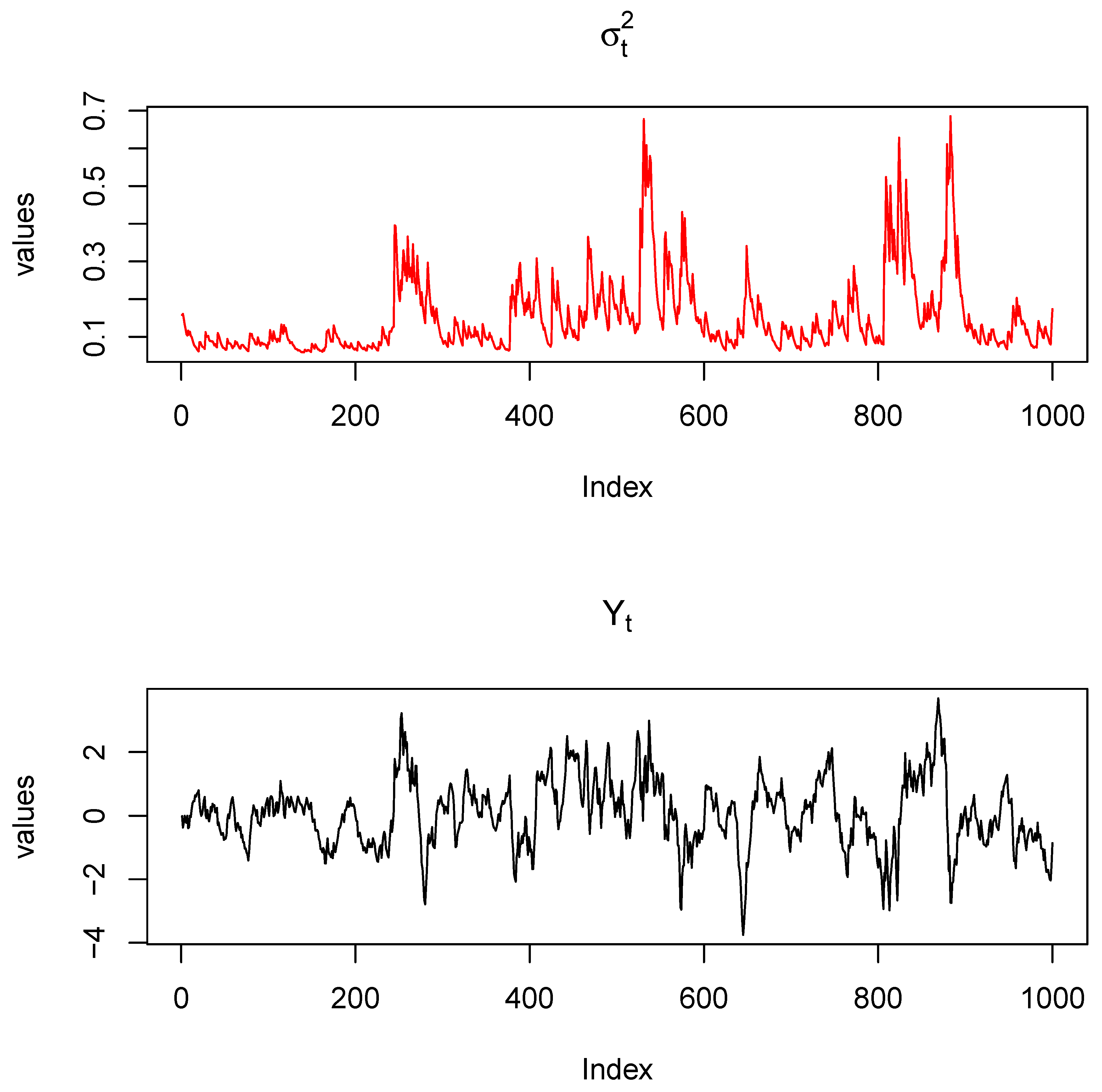
Figure 2.
Empirical distribution of the GARCH parameters , and . The DGP is a MARMA(1,1,0,0)-GARCH(1,1) with student’s t with 4.5 degrees of freedom.
Figure 2.
Empirical distribution of the GARCH parameters , and . The DGP is a MARMA(1,1,0,0)-GARCH(1,1) with student’s t with 4.5 degrees of freedom.
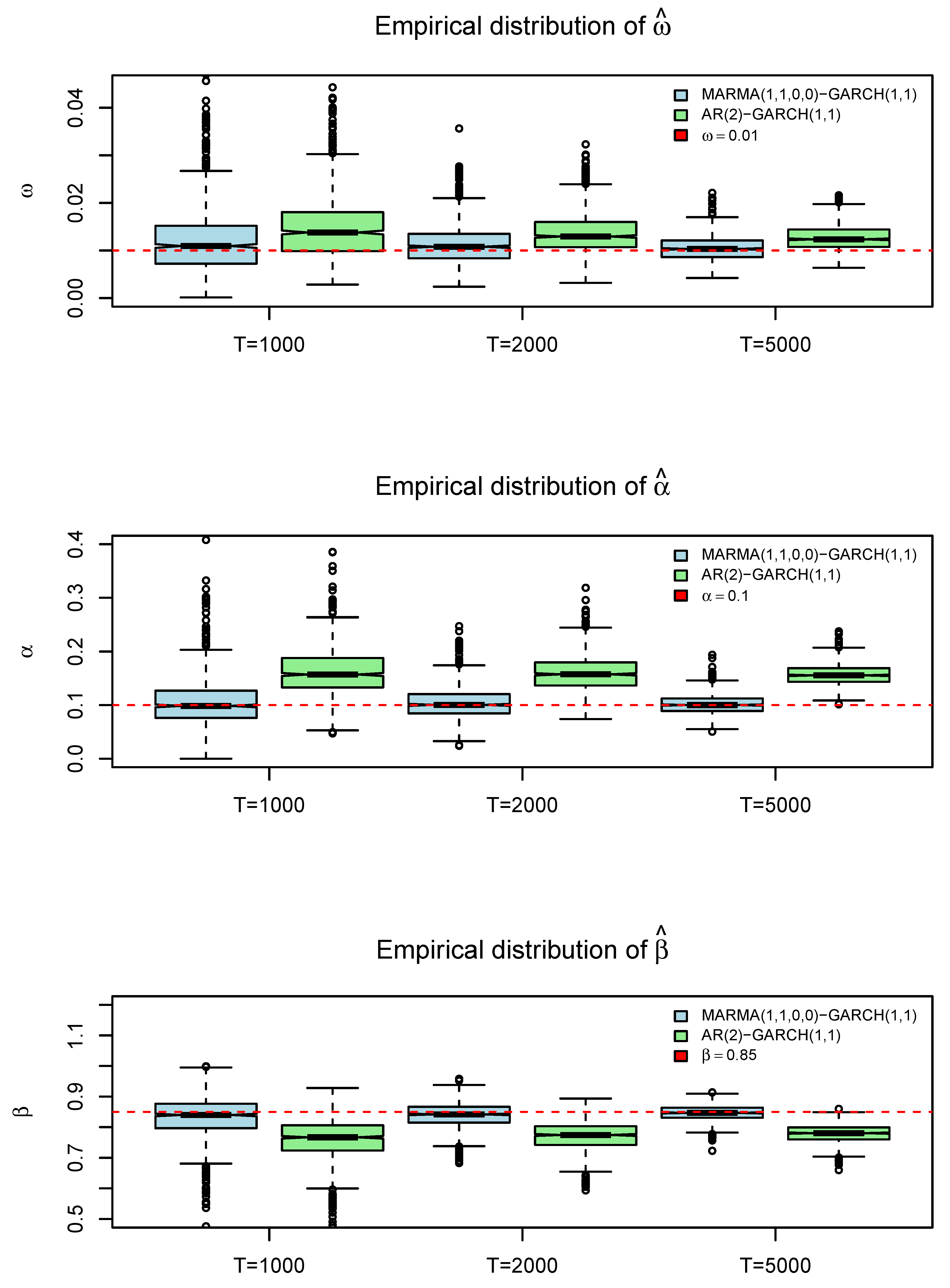
Figure 3.
Bitcoin and Ethereum price in USD.
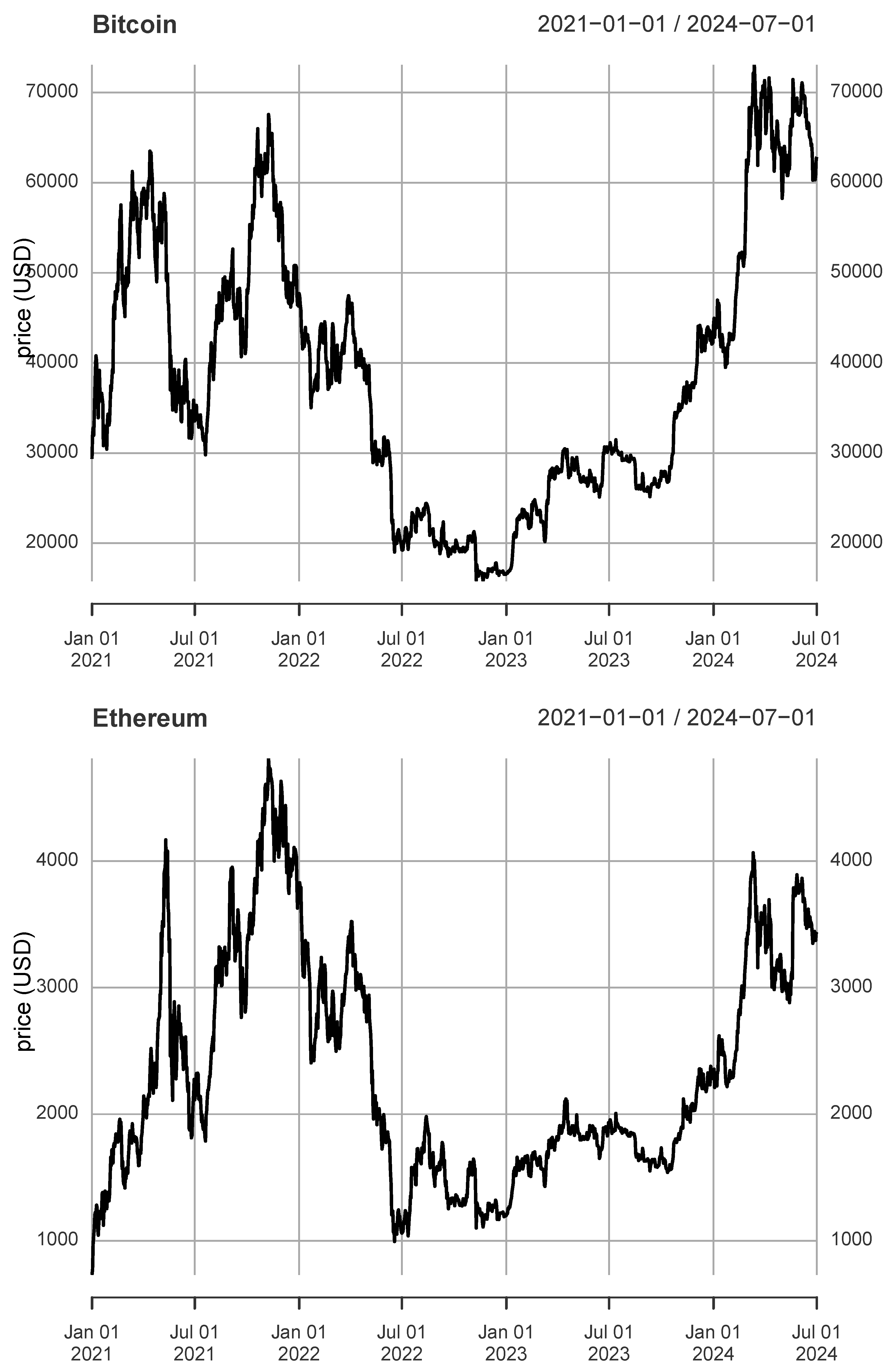
Figure 4.
Detrenden Bitcoin Price.
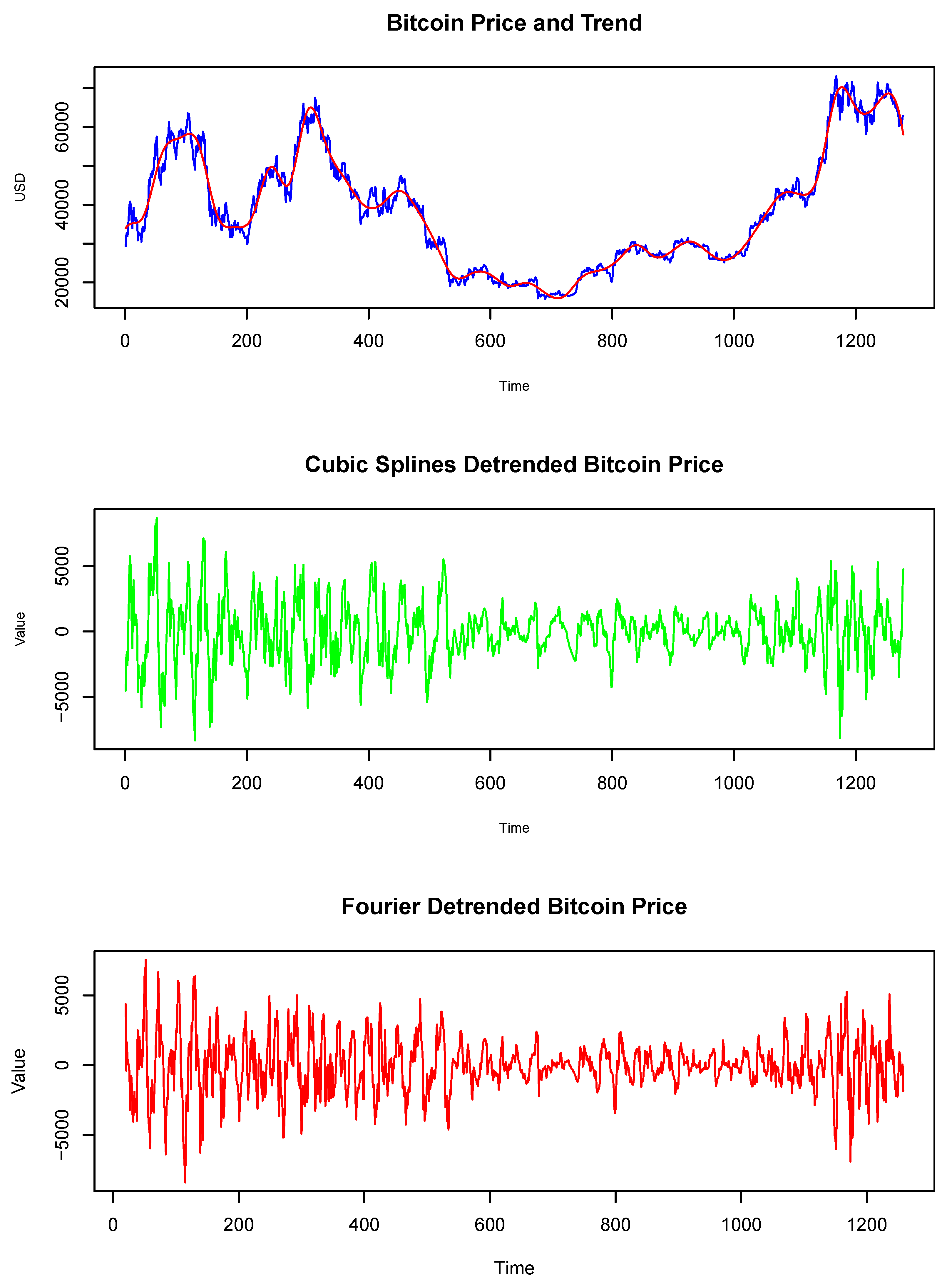
Figure 5.
Detrenden Ethereum Price.
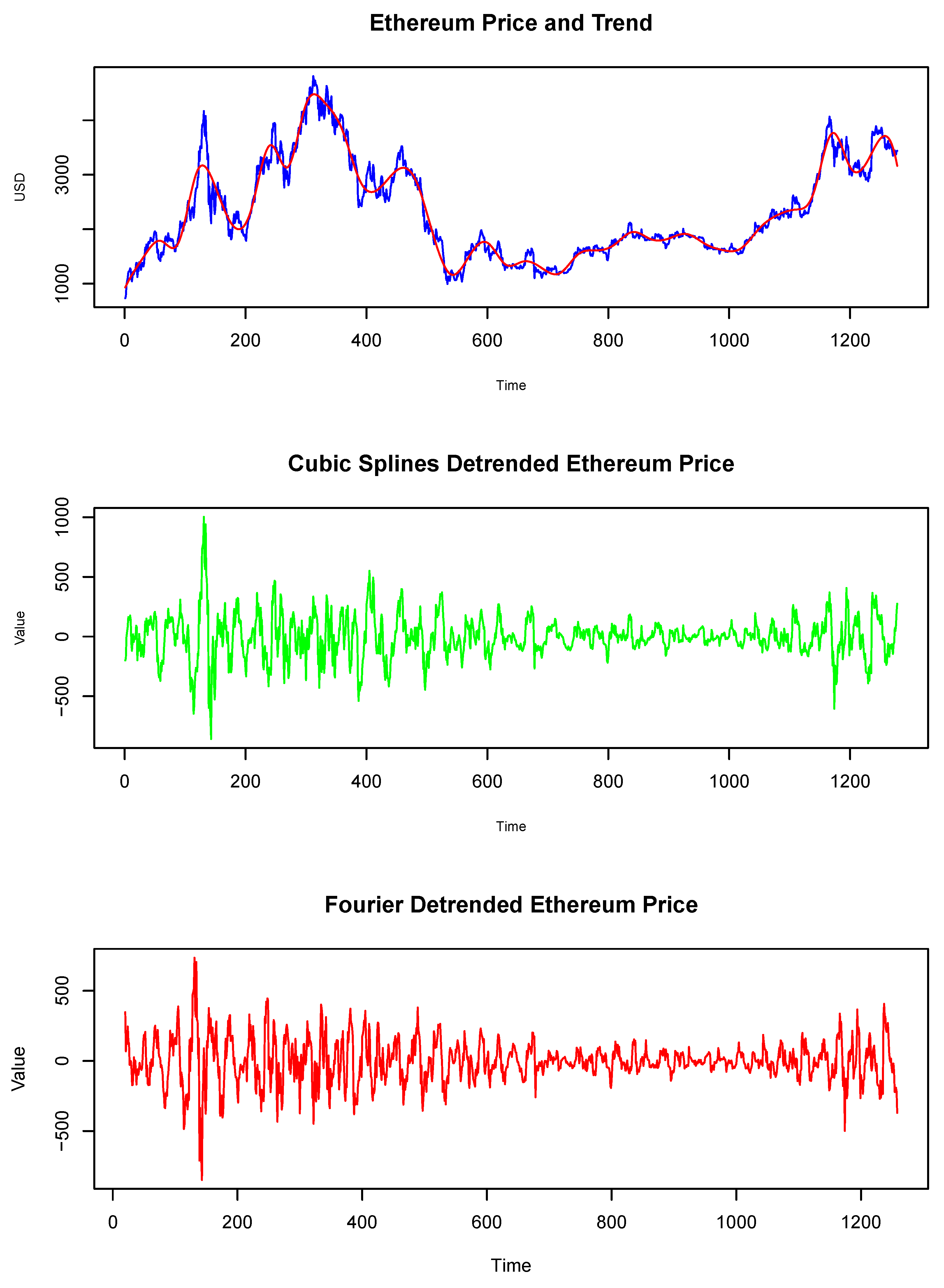
Figure 6.
Conditional volatility Bitcoin and Ethereum.
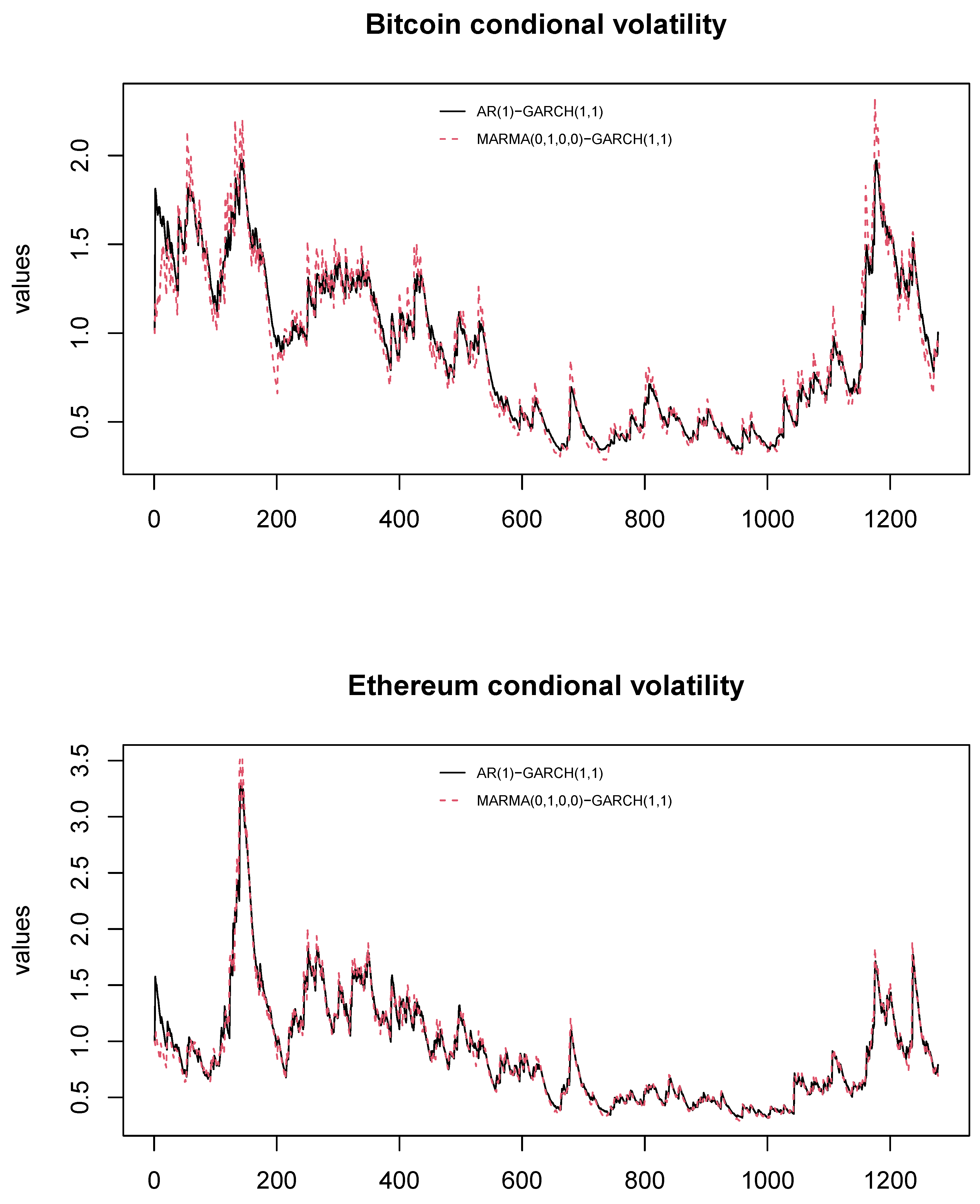

Table 1.
Bias and RMSE for GARCH(1,1) Parameter Estimates under Different Distributions. True parameters: , , .
Table 1.
Bias and RMSE for GARCH(1,1) Parameter Estimates under Different Distributions. True parameters: , , .
| Bias | RMSE | |||||||||||
|---|---|---|---|---|---|---|---|---|---|---|---|---|
| Whittle Estimation | Maximum Likelihood | Whittle Estimation | Maximum Likelihood | |||||||||
| T | ||||||||||||
| Distribution: Exp(1) | ||||||||||||
| 1000 | 0.089 | -0.030 | -0.030 | 0.020 | 0.006 | -0.020 | 0.288 | 0.073 | 0.182 | 0.067 | 0.063 | 0.081 |
| 2000 | 0.076 | -0.028 | -0.016 | 0.010 | 0.006 | -0.011 | 0.163 | 0.049 | 0.100 | 0.030 | 0.028 | 0.035 |
| 5000 | 0.073 | -0.024 | -0.016 | 0.002 | 0.000 | -0.002 | 0.115 | 0.032 | 0.075 | 0.010 | 0.011 | 0.013 |
| Distribution: Student’s t (8) | ||||||||||||
| 1000 | 0.055 | -0.018 | -0.015 | 0.014 | -0.001 | -0.009 | 0.136 | 0.039 | 0.092 | 0.034 | 0.026 | 0.036 |
| 2000 | 0.043 | -0.011 | -0.013 | 0.007 | 0.001 | -0.005 | 0.064 | 0.030 | 0.050 | 0.015 | 0.012 | 0.015 |
| 5000 | 0.039 | -0.008 | -0.012 | 0.001 | -0.001 | 0.000 | 0.042 | 0.016 | 0.031 | 0.006 | 0.005 | 0.006 |
| Distribution: Student’s t (4.5) | ||||||||||||
| 1000 | 0.103 | -0.023 | -0.039 | 0.020 | 0.003 | -0.017 | 0.248 | 0.054 | 0.152 | 0.046 | 0.039 | 0.051 |
| 2000 | 0.079 | -0.024 | -0.020 | 0.012 | 0.004 | -0.012 | 0.120 | 0.033 | 0.072 | 0.022 | 0.022 | 0.026 |
| 5000 | 0.054 | -0.024 | -0.008 | 0.003 | 0.000 | -0.003 | 0.063 | 0.019 | 0.045 | 0.007 | 0.008 | 0.009 |
| Distribution: skew-t(4.5,1.5) | ||||||||||||
| 1000 | 0.128 | -0.022 | -0.051 | 0.021 | 0.007 | -0.022 | 0.327 | 0.064 | 0.166 | 0.049 | 0.050 | 0.062 |
| 2000 | 0.107 | -0.021 | -0.033 | 0.008 | 0.007 | -0.011 | 0.197 | 0.034 | 0.095 | 0.021 | 0.024 | 0.027 |
| 5000 | 0.103 | -0.019 | -0.037 | 0.004 | 0.004 | -0.005 | 0.097 | 0.025 | 0.065 | 0.009 | 0.011 | 0.012 |
Table 2.
Estimating the parameters of the MARMA(1,1,0,0)-GARCH(1,1) process with , , , and beta=0.85. The mean and the standard deviation are presented.
Table 2.
Estimating the parameters of the MARMA(1,1,0,0)-GARCH(1,1) process with , , , and beta=0.85. The mean and the standard deviation are presented.
| DGP: MARMA(1,1,0,0)-GARCH(1,1) | ||||||||||
|---|---|---|---|---|---|---|---|---|---|---|
| Mean | ||||||||||
| AR(2)-GARCH(1,1) | MARMA(1,1,0,0)-GARCH(1,1) | |||||||||
| T | ||||||||||
| Dist: Exp(1) | ||||||||||
| 1000 | 0.893 | -0.143 | 0.023 | 0.358 | 0.542 | 0.675 | 0.218 | 0.012 | 0.108 | 0.828 |
| 2000 | 0.896 | -0.142 | 0.022 | 0.359 | 0.549 | 0.686 | 0.211 | 0.011 | 0.106 | 0.836 |
| 5000 | 0.899 | -0.141 | 0.021 | 0.359 | 0.558 | 0.695 | 0.204 | 0.011 | 0.104 | 0.843 |
| Dist: Student’s t(8) | ||||||||||
| 1000 | 0.896 | -0.141 | 0.013 | 0.115 | 0.820 | 0.685 | 0.211 | 0.012 | 0.102 | 0.836 |
| 2000 | 0.900 | -0.141 | 0.011 | 0.115 | 0.828 | 0.694 | 0.206 | 0.011 | 0.100 | 0.844 |
| 5000 | 0.899 | -0.140 | 0.011 | 0.115 | 0.830 | 0.698 | 0.201 | 0.010 | 0.101 | 0.846 |
| Dist: Student’s t(4.5) | ||||||||||
| 1000 | 0.897 | -0.140 | 0.016 | 0.180 | 0.736 | 0.685 | 0.212 | 0.013 | 0.111 | 0.825 |
| 2000 | 0.898 | -0.142 | 0.014 | 0.177 | 0.751 | 0.689 | 0.209 | 0.012 | 0.108 | 0.834 |
| 5000 | 0.901 | -0. 142 | 0.013 | 0.175 | 0.756 | 0.695 | 0.205 | 0.011 | 0.104 | 0.842 |
| Dist: Skew-t(4.5, 1.5) | ||||||||||
| 1000 | 0.897 | -0.144 | 0.017 | 0.222 | 0.683 | 0.678 | 0.219 | 0.012 | 0.111 | 0.825 |
| 2000 | 0.897 | -0.143 | 0.016 | 0.217 | 0.699 | 0.684 | 0.213 | 0.012 | 0.109 | 0.832 |
| 5000 | 0.899 | -0.140 | 0.015 | 0.214 | 0.708 | 0.695 | 0.204 | 0.011 | 0.104 | 0.843 |
| Standard Deviation | ||||||||||
| AR(2)-GARCH(1,1) | MARMA(1,1,0,0)-GARCH(1,1) | |||||||||
| T | ||||||||||
| Dist: Exp(1) | ||||||||||
| 1000 | 0.048 | 0.047 | 0.009 | 0.087 | 0.116 | 0.064 | 0.089 | 0.009 | 0.060 | 0.093 |
| 2000 | 0.036 | 0.036 | 0.006 | 0.060 | 0.077 | 0.048 | 0.065 | 0.005 | 0.041 | 0.054 |
| 5000 | 0.025 | 0.024 | 0.004 | 0.040 | 0.049 | 0.030 | 0.041 | 0.003 | 0.028 | 0.033 |
| Dist: Student’s t(8) | ||||||||||
| 1000 | 0.040 | 0.039 | 0.006 | 0.032 | 0.055 | 0.059 | 0.076 | 0.006 | 0.031 | 0.054 |
| 2000 | 0.032 | 0.030 | 0.004 | 0.021 | 0.034 | 0.038 | 0.053 | 0.004 | 0.021 | 0.033 |
| 5000 | 0.020 | 0.019 | 0.002 | 0.013 | 0.021 | 0.024 | 0.033 | 0.002 | 0.013 | 0.020 |
| Dist: Student’s t(4.5) | ||||||||||
| 1000 | 0.047 | 0.047 | 0.009 | 0.050 | 0.088 | 0.066 | 0.089 | 0.008 | 0.053 | 0.078 |
| 2000 | 0.037 | 0.037 | 0.005 | 0.036 | 0.053 | 0.049 | 0.068 | 0.005 | 0.040 | 0.050 |
| 5000 | 0.026 | 0.025 | 0.003 | 0.021 | 0.032 | 0.032 | 0.044 | 0.003 | 0.024 | 0.032 |
| Dist: Skew-t(4.5, 1.5) | ||||||||||
| 1000 | 0.050 | 0.048 | 0.009 | 0.063 | 0.103 | 0.067 | 0.090 | 0.010 | 0.065 | 0.094 |
| 2000 | 0.039 | 0.038 | 0.005 | 0.040 | 0.063 | 0.051 | 0.070 | 0.006 | 0.046 | 0.061 |
| 5000 | 0.028 | 0.027 | 0.003 | 0.025 | 0.037 | 0.036 | 0.049 | 0.003 | 0.028 | 0.036 |
Table 3.
Descriptive statistics of the prices and the detrended prices.
| Mean | Std. Dev. | Min | Max | Skewness | Kurtosis | |
|---|---|---|---|---|---|---|
| Bitcoin | ||||||
| Price | 38384.650 | 15015.490 | 15787.280 | 73083.500 | 0.473 | 2.188 |
| Cubic Splines | 0.000 | 2190.830 | -8347.694 | 8712.283 | 0.034 | 4.210 |
| Fourier | 0.000 | 2177.264 | -19449.880 | 12595.560 | -0.874 | 13.362 |
| Ethereum | ||||||
| Price | 2324.600 | 888.746 | 730.368 | 4812.087 | 0.680 | 2.439 |
| Cubic Splines | 0.000 | 172.251 | -858.576 | 1003.885 | 0.193 | 6.543 |
| Fourier | 0.000 | 175.118 | -1433.179 | 1162.614 | -0.434 | 13.595 |
Table 4.
Estimated parameters of the MARMA(0,1,0,0)-GARCH(1,1) and the causal representation AR(1)-GARCH(1,1). The Ljung-box test for the residuals, and the Mcleod-Li test for the standardized residuals
Table 4.
Estimated parameters of the MARMA(0,1,0,0)-GARCH(1,1) and the causal representation AR(1)-GARCH(1,1). The Ljung-box test for the residuals, and the Mcleod-Li test for the standardized residuals
| Bitcoin | Ethereum | |||||||
|---|---|---|---|---|---|---|---|---|
| Detrending method | ||||||||
| Cubic splines | Fourier | Cubic splines | Fourier | |||||
| Noncausal model | causal model | Noncausal model | causal model | Noncausal model | causal model | Noncausal model | causal model | |
| Parameters | MARMA(0,1,0,0) -GARCH(1,1) |
AR(1) -GARCH(1,1) |
MARMA(0,1,0,0) -GARCH(1,1) |
AR(1) -GARCH(1,1) |
MARMA(0,1,0,0) -GARCH(1,1) |
AR(1) -GARCH(1,1) |
MARMA(0,1,0,0) -GARCH(1,1) |
AR(1) -GARCH(1,1) |
| , | 0.8115 (0.0197) |
0.8115 (0.0197) |
0.8341 (0.0157) |
0.8341 (0.0157) |
0.8243 (0.1580) |
0.8243 (0.1580) |
0.8395 (0.0154) |
0.8395 (0.0154) |
| 0.0048 (0.0017) |
0.0029 (0.0010) |
0.0035 (0.0016) |
0.0031 (0.0011) |
0.0053 (0.0021) |
0.0056 (0.0017) |
0.0065 (0.0020) |
0.0057 (0.0018) |
|
| 0.0952 (0.0179) |
0.0564 (0.0106) |
0.0717 (0.0215) |
0.0593 (0.0117) |
0.0937 (0.0195) |
0.0828 (0.0147) |
0.1142 (0.0208) |
0.0856 (0.0156) |
|
| 0.9037 (0.0171) |
0.9406 (0.0102) |
0.9274 (0.0210) |
0.9382 (0.0111) |
0.9053 (0.0187) |
0.9137 (0.0141) |
0.8847 (0.0297) |
0.91158 (0.0149) |
|
| Residuals: Ljung Box test p-values | ||||||||
| Lag(1) | 0.7320 | 0.6234 | 0.3571 | 0.6033 | 0.5967 | 0.6533 | 0.4724 | 0.8152 |
| Lag(2) | 0.3611 | 0.2300 | 0.3124 | 0.1920 | 0.3602 | 0.1375 | 0.2636 | 0.1378 |
| Lag(3) | 0.2495 | 0.1177 | 0.1752 | 0.1663 | 0.1543 | 0.1506 | 0.0768 | 0.0861 |
| Lag(4) | 0.1799 | 0.1193 | 0.1608 | 0.1393 | 0.4288 | 0.1074 | 0.2514 | 0.1522 |
| Lag(5) | 0.2680 | 0.1801 | 0.2524 | 0.2210 | 0.1006 | 0.2217 | 0.1296 | 0.2971 |
| Standardized residuals: Mcleod-Li test p-values | ||||||||
| Lag(1) | 0.5715 | 0.4675 | 0.2073 | 0.3690 | 0.7695 | 0.7769 | 0.6491 | 0.9418 |
| Lag(2) | 0.7797 | 0.4635 | 0.4348 | 0.4882 | 0.8757 | 0.8125 | 0.8982 | 0.9142 |
| Lag(3) | 0.3872 | 0.2529 | 0.3059 | 0.3532 | 0.7137 | 0.5604 | 0.5430 | 0.5474 |
| Lag(4) | 0.5366 | 0.3933 | 0.4488 | 0.5099 | 0.8478 | 0.6703 | 0.6943 | 0.6602 |
| Lag(5) | 0.6540 | 0.3478 | 0.5191 | 0.5179 | 0.6248 | 0.4927 | 0.7015 | 0.4562 |
Disclaimer/Publisher’s Note: The statements, opinions and data contained in all publications are solely those of the individual author(s) and contributor(s) and not of MDPI and/or the editor(s). MDPI and/or the editor(s) disclaim responsibility for any injury to people or property resulting from any ideas, methods, instructions or products referred to in the content. |
© 2025 by the authors. Licensee MDPI, Basel, Switzerland. This article is an open access article distributed under the terms and conditions of the Creative Commons Attribution (CC BY) license (http://creativecommons.org/licenses/by/4.0/).
Copyright: This open access article is published under a Creative Commons CC BY 4.0 license, which permit the free download, distribution, and reuse, provided that the author and preprint are cited in any reuse.


