
Submitted:
06 January 2025
Posted:
07 January 2025
You are already at the latest version
Abstract
This paper presents a calibration technique for the Intelligent Driver Model (IDM) car-following model that considers the physical interpretation of each parameter. Using an instrumented vehicle, trajectory data was gathered for a group of Portuguese drivers. The data included various basic scenarios, such as unrestricted acceleration and deceleration maneuvers, as well as following other cars in steady-state conditions. The calibration process involved two steps. In the first step, specific parameters that have clear physical interpretations were manually adjusted to accurately reproduce the speed patterns of basic driving scenarios. In the second step, the obtained results were used to establish the limits of values for a simultaneous calibration procedure. The results demonstrate that the calibration procedure enables precise replication of the actual trajectories. Nevertheless, the model validation results indicate that calibrating without limitations on the parameter search space produces estimates with greater explanatory capability, contradicting previous research and supporting the need for additional analyses.
Keywords:
Car-following
; Calibration
; Lidar
; Intelligent Driver Model
1. Introduction
The car-following (CF) model is a fundamental component of microscopic traffic simulation tools, as it represents the longitudinal movement of cars. CF models aim to accurately replicate the specific driving patterns of individual drivers as they follow another vehicle in a particular network simulation. Several CF models have been developed in recent decades, each based on different driving strategies. These strategies are typically classified as stimulus-based, safety distance, desired measures, optimal velocity, and psychophysical models [1].
Each of these CF models is derived from a mathematical formulation that incorporates multiple parameters. Calibrating these parameters is a challenging task that is of great interest to traffic researchers. If the parameters are not properly calibrated, the model may inaccurately represent a car's movement and lead to incorrect conclusions.
While several methods have been suggested to address this issue, many experts believe that the most accurate way to calibrate CF models is by using vehicle trajectory data. This data tracks the positions, speeds, and distances between the leading and following vehicles over time as they move along a road [2,3]. However, obtaining trajectory data from real-world conditions is often difficult, and the calibration procedures for CF and adaptive cruise control systems are usually expensive and complex. This may explain why only a small percentage (9%) of recent studies have focused on this topic [4].
This work introduces a simple, efficient, and cost-effective method for calibrating a specific CF model, the Intelligent Driver Model (IDM), using trajectory data from real traffic. In the rest of this document, Chapter 2 presents a brief overview of the advancements in the calibration techniques of CF models. Chapter 3 introduces the IDM and emphasizes the physical meanings and properties of all model parameters that are adjustable in the calibration process of the IDM. Chapter 4 provides a detailed description of the methodology employed to gather and analyze field data on a group of individual drivers, which ultimately formed the basis of our study's trajectory data. Chapter 5 outlines the sequential calibration procedures used to estimate reasonable boundary values for all parameters and explains the simultaneous calibration and validation tasks in relation to typical driving conditions. Chapter 6 contains the overall findings of the study.
2.2. Literature Review
The calibration and validation of microscopic traffic simulation models have advanced to improve the accuracy and realism of traffic dynamics representation. Some authors have presented calibration procedures that rely on macroscopic variables [5,6]. The fundamental concept of this approach is to modify the variables of a specific CF model based on field data that represents steady-state conditions of road traffic (such as traffic flow, speed, and density) collected from loop detectors or similar devices. Other researchers combined macroscopic speed-flow graphs and vehicle trajectory data to calibrate and validate model parameters, specifically through the reduction of the search space and the number of potential solutions [7,8].
Two major conclusions can be drawn from these studies. First, driver behavior changes depending on the road environment (e.g., increased following distance in tunnels), so car-following parameters should be adjusted to account for these differences [9]. Second, while methods using macroscopic loop detector data are useful, they fall short in capturing the detailed interactions between individual vehicles. Adding microscopic data, like vehicle trajectories, improves the accuracy of calibration methods.
Vehicle trajectories are commonly obtained using driving simulators [10], instrumented vehicles [11,12,13], or aerial images captured by video cameras placed on tall buildings, helicopters, or drones [14,15]. Some data sets are managed by transportation authorities and are available for research under specific conditions, such as the Strategic Highway Research Program's naturalistic driving study focused on US freeways [16].
One influential study by Brockfeld & Wagner [17] examined ten different microscopic traffic flow models. They used data collected from cars equipped with DGPS technology on a test track in Japan, creating a controlled environment for studying driver behavior. Their approach involved inputting the lead car's data into each model to predict the following car's headway, then comparing these simulated headways with actual measurements. The calibration results, which showed errors between 12% and 17%, underscored the significant impact of individual driver behavior on traffic flow.
Kesting & Treiber [2] developed a calibration technique for car-following models using trajectory data from a vehicle with radar sensors. They applied a genetic algorithm to minimize the differences between observed and simulated trajectories.
Ossen & Hoogendoorn [18] highlighted the impact of measurement errors in trajectory data on the calibration of car-following models. They emphasized the need for careful data preprocessing and methods to reduce errors, as inaccuracies can distort parameter estimation and limit the models’ general applicability. This aligns with the findings of Brockfeld & Wagner [17], who warned about the risks of "overfitting," where models become overly tailored to specific training data, thereby restricting their applicability to other scenarios. Another related debate in the field concerns whether parameters should be calibrated sequentially (individually in a set order) or simultaneously (adjusted together) [13,4,19].
This study presents a simple and cost-effective method for collecting trajectory data, suitable for small research teams and projects, and introduces a two-step process for calibrating the IDM car-following model. The method involves an initial partial sequential calibration followed by simultaneous constrained optimization.
3. The Intelligent Driver Model
3.1. Overview
The Intelligent Driver Model is a simple, deterministic, time-continuous model which belongs to the family of optimal velocity models [20]. Developed in 2000 [21] it includes specifications that make it collision-free. Over time, IDM has evolved into several variants [22], becoming one of the most widely used CF models. Its popularity stems from its superior performance in representing vehicle CF behavior across all single-lane traffic situations, including the driving behavior of automated vehicles [23]. Moreover, IDM's collision-free design, simplicity in calibrating model parameters using empirical data, fast numerical simulations, and the existence of a corresponding macroscopic model [24] further contribute to its widespread adoption. For these reasons, IDM is the CF model employed in the present work.
3.2. Model Structure
The IDM has the following dynamic properties [22]:
- The following vehicle acceleration is a strictly decreasing function of its own speed; in free road conditions, the vehicle accelerates to the desired speed.
- The following vehicle acceleration is a strictly decreasing function of the relative distance from the leading vehicle.
- The following vehicle acceleration grows with the speed of the leading vehicle.
- The following and leading vehicles keep a minimum distance (bumper-to-bumper distance); there is no reverse movement even if any event leads to a relative distance between the follower and leading vehicles less than the minimum distance.
Altogether, it implies that the IDM is a complete CF model in the sense that it has a distinctive steady-state flow density.
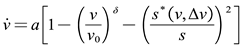
The model equations are expressed mathematically as coupled ordinary differential equations, that is, the subject vehicle v (speed) and its derivative dv/dt (acceleration, hereon represented by  are calculated simultaneously. The IDM acceleration is calculated as presented in Equation 1:
 where,
are calculated simultaneously. The IDM acceleration is calculated as presented in Equation 1:
 Acceleration [m/s2]
a Maximum acceleration [m/s2]
v Speed of the following vehicle [m/s]
v0 Desired speed [m/s]
δ Exponent factor
s Actual distance between vehicles (bumper-to-bumper distance) [m]
s* Desired distance between vehicles [m]
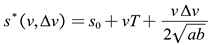
The acceleration equation has two major terms. The following vehicle acceleration under free road conditions is described in the first term 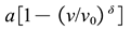 by comparing the current speed v, to the desired speed, v0. The second term compares the actual distance between vehicles s with the desired distance s*. If s ≈ s* the output acceleration is roughly zero. The IDM desired distance between vehicles is given by Equation 2:
 where,
by comparing the current speed v, to the desired speed, v0. The second term compares the actual distance between vehicles s with the desired distance s*. If s ≈ s* the output acceleration is roughly zero. The IDM desired distance between vehicles is given by Equation 2:
s* Desired distance between vehicles [m]
s0 Minimum distance between vehicles [m]
v Speed of the following vehicle [m/s]
T Desired safety time headway to the vehicle in front [s]
Δv Speed difference between vehicles [m/s]
a Maximum acceleration [m/s2]
b Maximum braking deceleration [m/s2]
Thus, the following vehicle's acceleration at a given instant t depends on its own speed v, speed difference Δv to the leading vehicle, and distance s. Overall, the IDM parameters that are adjustable to represent specific driving behaviors are: a, b, δ , v0, s0, and T.
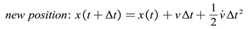
To simulate vehicle trajectories, a numerical integration scheme is necessary. The term "integration" refers to the process of estimating the solution to the coupled ordinary differential equations that characterize the time-continuous car-following model. In practice it means that over a finite time interval Δt, the speed v, position x, and distance s between the vehicles are updated under the assumption of a constant acceleration. The ballistic method, a well-known standard integration scheme used in this work [25], is as follows:

 where,
 New updated speed of the following vehicle [m/s]
 Speed of the following vehicle [m/s] at time t
 IDM Acceleration [m/s2] calculated at time t
 New updated position of the following vehicle [m]
 Position of the following vehicle [m] at time t
v Speed of the following vehicle [m/s]
3.3. Estimation Approach for Particular Cases
Each IDM parameter represents a specific element of driving behavior, enabling the development of a combined calibration procedure (sequential + simultaneous) in two stages:
- Phase 1: Seeks to precisely adjust the IDM parameters associated with a specific set of basic driving scenarios conducted in a controlled environment.
- Phase 2: involves the simultaneous adjustment of all parameters using an automatic calibration procedure. This procedure focusses on typical driving scenarios in urban areas and is based on the results obtained in Phase 1, which established boundaries and initial estimates of the IDM parameters.
The driving cases considered for Phase 1 are: i) car-following in steady-state conditions, ii) unconstrained acceleration from a standstill, iii) approaching a stopped vehicle.
3.3.1. Car-Following in Steady-State Conditions
When following a leading vehicle at a constant speed 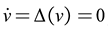 , the bumper-to-bumper distance between vehicles s is determined by Equation 2. If the leader vehicle travels at speeds considerably lower than the follower's desired speed
  , the distance between them varies linearly with speed and is mainly influenced by s0 and T. The parameter s0 can be considered as the distance between two consecutively stopped vehicles.
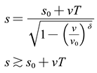
, the bumper-to-bumper distance between vehicles s is determined by Equation 2. If the leader vehicle travels at speeds considerably lower than the follower's desired speed , the distance between them varies linearly with speed and is mainly influenced by s0 and T. The parameter s0 can be considered as the distance between two consecutively stopped vehicles.
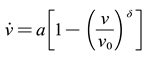
3.3.2. Unconstrained Acceleration from a Standstill
When the vehicle is travelling in the absence of surrounding traffic or at a significant distance from the leader (s → ∞), Equation 1 can be simplified. Note that the vehicle achieves its maximum acceleration a when it begins to accelerate from a standstill position. The acceleration subsequently diminishes as the velocity of the vehicle rises and ultimately reaches zero as the vehicle approaches the target speed v0. The exponent δ governs the decrease in acceleration. As the value increases, the rate of acceleration decreases more smoothly. As a result, the limit δ → ∞ is a bilinear speed diagram. In this scenario, the braking deceleration term is zero, and the vehicle acceleration can be easily calculated using the following equation:
3.3.3. Approaching a Stopped Vehicle
When a vehicle is moving at a constant velocity and detects a slower or stationary car ahead, it will apply the brakes or decrease its speed to avoid any potential collisions. The vehicle's trajectory in this scenario is affected by all IDM parameters, which complicates the process of individual calibration. However, because the parameters a, δ, T, and s0 can be estimated from the driving scenarios previously examined, their respective values can be treated as constant. This means that the maneuver of approaching a stationary vehicle is primarily influenced by the maximum deceleration, b.
4. Data collection and Preparation
4.1. Sample and Vehicle Instrumentation
This study involved data collection from various vehicles and drivers. The vehicles used included a 2021 Hyundai Bayon with a manual transmission, a 2005 Opel Corsa with a manual transmission, and a 2015 Mercedes C220 with an automatic transmission. The study sample comprised five drivers, who were students and professors from the Polytechnic Institute of Viseu, Portugal. These participants, representing both genders, were aged between 23 and 53 years and had prior driving experience. Data was gathered on their car-following behavior using leader–follower pairs, with the follower vehicles equipped with a datalogger (DL1 Club, Race Technology Ltd) paired with a Lidar (ULS, Laser Technology Inc.) – see Figure 1.
The datalogger allows for the collection of speed measurements with a precision of less than 0.1 km/h and positional measurements with a precision of 3 m (circular error probability) thanks to its internal accelerometers and a 20 Hz GPS receiver. The total expense for this equipment is below 2,500 €. The coupled Lidar was employed to measure the bumper-to-bumper distance to the vehicle in front. However, as the equipment was placed inside the follower car, it was necessary to subtract the distance between the Lidar's location and the vehicle bumper to determine the precise bumper-to-bumper distance.
4.2. Route and Experimental Procedures
The experiment was conducted on a diverse urban route spanning 4.4 km in each direction (refer to Figure 2). The route included different types of roads: sections 1-2 and 3-4 were arterial roads with a central divider, while section 2-3 was a distribution road. Starting at the university campus, drivers were instructed to follow the lead vehicle through sections 1 to 4 while driving normally. The lead driver maintained various steady speeds along the route, all relatively low, to prompt the follower vehicle to engage in longitudinal following maneuvers. In some instances, the leader's speed exceeded the follower vehicle's preferred speed, causing a disruption in the speed-distance elastic response. Section 4-5 was specifically designated for acceleration and deceleration maneuvers: drivers were instructed to accelerate from a standstill to a steady desired speed and then decelerate to a complete stop. Drivers 1 and 3-5 performed these maneuvers while driving normally, whereas driver 2 repeated the acceleration/deceleration maneuvers 20 times, adopting different driving styles – comfortable, normal, and aggressive – to determine realistic variation ranges for the associated IDM parameters.
4.3. Data Preparation
The obtained database comprises time series data that includes the follower vehicle's position, speed, acceleration, and distance from the leader. Initially, these data were analyzed using the Race Technology software (refer to Figure 3) and subsequently exported in ".mat" format for further analysis in Matlab. This software was used to filter the data to remove outliers, such as Lidar detection failures, and resize it to a frequency of 4 Hz. This resulted in smaller files and faster optimization procedures.
5. Calibration Methodology
5.1. General Considerations
This work used a process called systematic estimation of optimal parameters to accurately calibrate the IDM model to observed car-following behaviour. Generally, each calibration process follows an optimisation framework that involves, at the very least, defining a measure of performance (MoP) and an objective function. [26].
A Measure of Performance (MoP) is a metric that highlights a specific aspect of car-following behavior. In the literature, various MoPs are used in optimization problems related to this behavior. Examples include the distance and time headway between two consecutive vehicles as well as the position and speed of the following vehicle. Based on recent studies [27,28], the kinematic measure with the higher magnitude (position) should be preferred. However, in this study case, we have opted for a metric of intermediate magnitude (speed) because it is the most traditionally favored metric.
The objective function, in this context, dictates whether the difference between the observed and simulated MoPs should be maximized or minimized, while also defining the relevant constraints. To achieve this, formulas like the Mean Absolute Error (MAE) or the GEH statistic are often utilized. However, due to its heightened sensitivity to small values, the Root Mean Square Error (RMSE) is particularly favored in car-following studies [26,29].
Therefore, the objective function seeks to minimize the Root Mean Square Error (RMSE) between the observed and simulated speeds of the following vehicle, as given below:
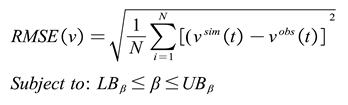 where,
RMSE Root Mean Square Error [m/s]
vsim Speed of the following vehicle estimated by the model [m/s]
vobs Speed of the following vehicle observed in the experiment [m/s]
N Observations number (time-steps or time interval)
β Solution vector (a, δ, b, s0, T, v0)
LBβ Vector of the minimum values admitted as solution
UBβ Vector of the maximum values admitted as solution
5.2. Sequential Calibration
5.2.1. Car-Following Under Steady-State Condition
Equation 6 establishes a nearly linear correlation between speed and distance in the context of steady-state car following. Therefore, for every driver, the speed and distance to the leader have been recorded in brief intervals (≈ 4 s), not necessarily consecutive, along the 1-4 route, where stationary conditions (consistent speed and distance) were observed.
Figure 4 displays the data points for speed-distance (v – s) and their corresponding linear regression lines. The defining features of these lines are their point of intersection and their inclination, which correspond to the values of s0 and T. The proximity of the points to the regression line indicates that each driver consistently follows a consistent driving style.
However, there is significant variation between drivers, as indicated by the dispersion of points in the overall graph. This variation aligns with the findings of Ossen & Hoogendoorn [31], who identified clear differences in speed-dependent desired headways and emphasized the stochastic nature of traffic.
Specifically, drivers 2 and 5 consistently maintain a significantly shorter distance to the leader compared to drivers 1, 3, and 4. Table 1 includes the outcomes of the calibration phase, specifically the average values of the parameters s0 and T, along with other described elements.
5.2.2. Acceleration and Deceleration Under Free-Flow Conditions
According to Equation 7, which governs acceleration maneuvers, the parameters a and δ regulate the evolution of speed until the desired speed v0 is reached. In the optimization problem v0 was manually assigned based on clear thresholds in the speed diagram, while a and δ were optimized for each maneuver. Figure 5 illustrates the model's predicted trajectory for two driver-vehicle combinations, one with automatic transmission (left panel, a = 2.03 m/s2, δ = 4.20, and v0 = 14.0 m/s) and the other with manual transmission (right panel, a = 2.06 m/s2, δ = 3.84, and v0 = 13.5 m/s). The model closely replicates the distance profile, with almost indistinguishable lines. Speeds were also predicted with high accuracy, although small deviations start to emerge due to the amplification of errors inherent in the first derivative of position, particularly in the manual transmission scenario. Predictions for acceleration, however, were less precise, as the second derivative further amplifies noise and minor discrepancies in the input data and model.
5.2.3. Deceleration
To calibrate the maximum deceleration parameter b, a similar procedure was followed, this time aiming to replicate the speed profile of an isolated vehicle from the moment it begins to decelerate until it comes to a stop. Given that all parameters have an impact on this profile, s0 was set to 0 (the leading vehicle is fictitious), and the parameters a, δ, and T were assigned the average values identified in the previous steps for the respective driver. The curve fitting was then performed solely by adjusting b. It is important to acknowledge that the impact of this parameter on the model's outcomes cannot be separated from the value of a (refer to Equation 2) meaning that the same deceleration behavior can be achieved through different a-b combinations. Figure 6 illustrates the kinematic profiles corresponding to a deceleration maneuver of driver 2 (a = 2.02 m/s2, δ = 2.40, T = 0.95, s0 = 0 → b = 2.08 m/s2). The results of this calibration phase, expressed as average values for each driver, can be found in Table 1. Note that desired speed values are not included, as these were chosen arbitrarily by the drivers during each maneuver.
5.3. Simultaneous Calibration
5.3.1. Parameter Domain
The estimates obtained in the previous section through the sequential calibration process were derived under specific conditions, namely unconstrained acceleration and deceleration maneuvers, and following a leader vehicle under steady conditions on a traffic-free road. Nevertheless, the primary objective consists in accurately representing driver conduct in urban settings, which are distinguished by a multitude of driving patterns and stimuli. Under these circumstances, all elements of CF models are involved, including parameters that are more challenging or unattainable to observe through simpler actions. The optimal parameters for representing these conditions are expected to be different from those that are best suited for simple maneuvers. Therefore, a simultaneous calibration process with local data is necessary. This optimization should be carefully limited for the following reasons:
- Unforeseen events frequently arise in real-world driving situations that are not accounted for in the model specifications (e.g., navigating intersections, distractions from mobile devices, abrupt braking, etc.). While these events should be excluded, there are instances where the analyst fails to detect them, resulting in their inclusion in the training data. This can introduce bias in the calibration process and yield unrealistic parameters.
- Occasionally, the calibration data is relevant to segments with minimal fluctuations in traffic conditions, which may result in impractical values for the less significant parameters.
To ensure that the calibration yields parameters accurately reflecting driver behavior based on the training data, while also performing well with independent data, our goal was to establish a practical range of values for each parameter. To achieve this, we concentrated on the variability of parameters for driver 2. As previously noted, driver 2 executed acceleration and deceleration maneuvers across a range of speeds, from very gentle to highly aggressive driving styles. For this driver, a specific range was determined for each parameter, defined as [LB, UB], where LB and UB represent the lower and upper bounds, set at the 15th and 85th percentiles of the results, respectively. The relationship between each percentile and the mean was then similarly applied to the other drivers.
To streamline data collection and reduce costs and time, the remaining drivers only performed maneuvers in normal driving mode, as shown in Table 1. This table includes a broader scope applicable to all drivers. This wider range is intended for use in an "unconstrained" calibration process, ensuring that the resulting parameters fall within a realistic and practical range.
5.3.2. Calibration and Cross-Validation
After establishing acceptable ranges for the different parameters, a simultaneous parameter calibration was conducted using optimization techniques, similar to the sequential calibration performed with the fmincon function. To streamline the presentation of findings, this analysis focused specifically on two drivers: driver 1 and driver 2. A standardized procedure was applied to each driver.
- Trajectory data, including kinematic variables and distance to the leader, was extracted for two large heterogeneous segments: outbound (1 → 4) and inbound (4 → 1). The periods at the beginning and end, where stable following conditions were not met, were excluded from the analysis.
- Parameter calibration was conducted for each segment using two optimization methods: a) constrained within the [LB, UB] intervals specified in Table 1; b) unconstrained, where no restrictions were placed on the parameter values (only physically plausible ranges were defined).
- Model validation was conducted on the complementary segments, meaning that parameters calibrated on the outbound segment were utilized to forecast behavior on the return segment and vice versa.
The results of this procedure are shown in Table 2. Furthermore, Figure 7 presents a graphical depiction of these findings for drivers 1 and 2. The diagram depicts the performance of the model on the inbound route when using parameters calibrated on the outbound route, and vice versa, using both constrained and unconstrained calibration methods.
5.4. Analysis and Discussion of Results
Upon initial analysis, it is evident that the IDM model accurately reproduces the actual speed profiles, thereby confirming the model's capability to simulate urban traffic. The RMSE values for a specific driver exhibit similarity between the calibration and validation segments, as anticipated due to the instruction given to drivers to maintain a normal driving style on both segments. Nevertheless, when assessing the impact of parameter restriction during the calibration process, an unexpected outcome is observed: the model typically exhibits superior performance against independent data (validation segment) when employing parameters derived from unconstrained calibration. As an illustration, when considering driver 1, the calibrated parameters with limitations on the outbound route yielded a RMSE of 1.64 m/s. Conversely, the estimated parameters without any restrictions resulted in an RMSE of 1.04 m/s. The unconstrained calibration mode resulted in solution sets where one or more parameters reached the boundary of the domain, enabling a more accurate alignment of the speed profile in both the calibration and validation segments.
This finding contradicts previous research [13,32], which suggested that parameters estimated with minimal restrictions are less effective than those within "realistic" ranges for predicting driver behavior in new situations, on validation segments. Given that unconstrained optimization occasionally yielded values that clearly fell outside the anticipated and realistic range, it is reasonable to speculate about the underlying causes for this outcome. One aspect could pertain to the circumstances in which the parameters a, b, and δ were estimated, specifically on a road without traffic, with the maneuvers being unrelated to a typical urban road setting. More likely, it could be that the calibration and validation conditions are not sufficiently different, thereby preventing the IDM model's limitations from being emphasized when excessively calibrated to extreme scenarios. The traffic conditions on both the outbound and return segments are very similar, and the lead vehicle driver consistently maintained a uniform driving style throughout the session. Hence, it is necessary to conduct thorough testing of the model under substantially varied circumstances prior to dismissing the requirement of appropriately restricting the parameters in accordance with their physical significance.
6. Conclusions
The analysis of the structure of the IDM car-following model revealed specific cases that support a sequential and individualized calibration process for its parameters. Building on these insights, a process for collecting and analyzing trajectories was conducted to calibrate and validate the model in an urban environment. For this purpose, a low-cost system (under €2500) comprising a datalogger and a LIDAR was employed. This system proved to be both practical and highly accurate.
The data collection session included five drivers and enabled the identification of plausible ranges of variation for the IDM parameters. These ranges were then used to limit a simultaneous calibration process for an urban route. The outcomes of this procedure were unexpected, as the parameters derived from unconstrained calibration yielded superior model performance in the validation sections. The variation in driving styles during different maneuvers and urban driving sessions, as well as the lack of diversity in the driving environment during calibration and validation segments, are the probable causes of this phenomenon.
Further development of this study is necessary to confirm the reasonableness of the parameter domains and to test the model's predictive capability in road environments significantly different from those used in the calibration.
Author Contributions
All the authors have contributed on each of the themes. All authors have read and agreed to the published version of the manuscript.
Funding
This research was partially funded by the project SAFEWAY, from the Polytechnic Institute of Viseu.
Institutional Review Board Statement
Not applicable.
Informed Consent Statement
Informed consent was obtained from all subjects involved in the study.
Data Availability Statement
Data are contained within the article.
Conflicts of Interest
The authors declare no conflicts of interest.
References
- Rodrigues, R.; Bastos Silva, A.; Vasconcelos, L.; Seco, Á. The Longitudinal Driving Behavior of a Vehicle Assisted with Lv2 Driving Automation: An Empirical Study. Journal of Advanced Transportation 2022, 2022, 3073393. [CrossRef]
- Kesting, A.; Treiber, M. Calibrating Car-Following Models by Using Trajectory Data: Methodological Study. Transportation Research Record 2008, 2088, 148–156. [CrossRef]
- Anil Chaudhari, A.; Srinivasan, K.K.; Rama Chilukuri, B.; Treiber, M.; Okhrin, O. Calibrating Wiedemann-99 Model Parameters to Trajectory Data of Mixed Vehicular Traffic. Transportation Research Record 2022, 2676, 718–735. [CrossRef]
- Punzo, V.; Zheng, Z.; Montanino, M. About Calibration of Car-Following Dynamics of Automated and Human-Driven Vehicles: Methodology, Guidelines and Codes. Transportation Research Part C: Emerging Technologies 2021, 128, 103165. [CrossRef]
- Rakha, H.; Wang, W. Procedure for Calibrating Gipps Car-Following Model. Transportation Research Record 2009, 2124, 113–124. [CrossRef]
- Barceló, J. Models, Traffic Models, Simulation, and Traffic Simulation. In Fundamentals of Traffic Simulation; Barceló, J., Ed.; Springer: New York, NY, 2010; pp. 1–62 ISBN 978-1-4419-6142-6.
- Menneni, S.; Sun, C.; Vortisch, P. Integrated Microscopic and Macroscopic Calibration for Psychophysical Car-Following Models.; 2009.
- Vasconcelos, L.; Seco, Á.; Silva, A.B. Hybrid Calibration of Microscopic Simulation Models. In Computer-based Modelling and Optimization in Transportation; de Sousa, J.F., Rossi, R., Eds.; Springer International Publishing: Cham, 2014; pp. 307–320 ISBN 978-3-319-04630-3.
- Rakha, H.; Gao, Y. Calibration of Steady-State Car-Following Models Using Macroscopic Loop Detector Data.; 2010;
- Berghaus, M.; Kallo, E.; Oeser, M. Car-Following Model Calibration Based on Driving Simulator Data to Study Driver Characteristics and to Investigate Model Validity in Extreme Traffic Situations. Transportation Research Record: Journal of the Transportation Research Board 2021, 2675, 036119812110326. [CrossRef]
- Brackstone, M.; Sultan, B.; McDonald, M. Motorway Driver Behaviour: Studies on Car Following. Transportation Research Part F: Traffic Psychology and Behaviour 2002, 5, 31–46. [CrossRef]
- Ranjitkar, P.; Nakatsuji, T.; Kawamura, A. Experimental Analysis of Car-Following Dynamics and Traffic Stability. Transportation Research Record 2005, 1934, 22–32. [CrossRef]
- Vasconcelos, L.; Neto, L.; Santos, S.; Silva, A.B.; Seco, Á. Calibration of the Gipps Car-Following Model Using Trajectory Data. Transportation Research Procedia 2014, 3, 952–961. [CrossRef]
- Coifman, B.; Li, L. A Critical Evaluation of the Next Generation Simulation (NGSIM) Vehicle Trajectory Dataset. Transportation Research Part B: Methodological 2017, 105, 362–377. [CrossRef]
- Hale, D.K.; Ghiasi, A.; Khalighi, F.; Zhao, D.; Li, X. (Shaw); James, R.M. Vehicle Trajectory-Based Calibration Procedure for Microsimulation. Transportation Research Record 2023, 2677, 1764–1781. [CrossRef]
- Medina, J.C.; Malekloo, A.; Kersavage, K.; Porter, R.J.; Liu, X.C.; University of Utah; VHB/Vanasse Hangen Brustlin, Inc. Verification and Calibration of Microscopic Traffic Simulation Using Driver Behavior and Car-Following Metrics for Freeway Segments; 2024;
- Brockfeld, E.; Wagner, P. Calibration and Validation of Microscopic Traffic Flow Models. In Proceedings of the Traffic and Granular Flow ’03; Hoogendoorn, S.P., Luding, S., Bovy, P.H.L., Schreckenberg, M., Wolf, D.E., Eds.; Springer: Berlin, Heidelberg, 2005; pp. 67–72.
- Ossen, S.; Hoogendoorn, S.P. Validity of Trajectory-Based Calibration Approach of Car-Following Models in Presence of Measurement Errors. Transportation Research Record 2008, 2088, 117–125. [CrossRef]
- Daguano, R.F.; Yoshioka, L.R.; Netto, M.L.; Marte, C.L.; Isler, C.A.; Santos, M.M.D.; Justo, J.F. Automatic Calibration of Microscopic Traffic Simulation Models Using Artificial Neural Networks. Sensors 2023, 23, 8798. [CrossRef]
- Ahmed, H.U.; Huang, Y.; Lu, P. A Review of Car-Following Models and Modeling Tools for Human and Autonomous-Ready Driving Behaviors in Micro-Simulation. Smart Cities 2021, 4, 314–335. [CrossRef]
- Treiber, M.; Hennecke, A.; Helbing, D. Congested Traffic States in Empirical Observations and Microscopic Simulations. Phys. Rev. E 2000, 62, 1805–1824. [CrossRef]
- Treiber, M.; Kesting, A. Car-Following Models Based on Driving Strategies. In Traffic Flow Dynamics: Data, Models and Simulation; Treiber, M., Kesting, A., Eds.; Springer: Berlin, Heidelberg, 2013; pp. 181–204 ISBN 978-3-642-32460-4.
- Zhang, D.; Chen, X.; Wang, J.; Wang, Y.; Sun, J. A Comprehensive Comparison Study of Four Classical Car-Following Models Based on the Large-Scale Naturalistic Driving Experiment. Simulation Modelling Practice and Theory 2021, 113, 102383. [CrossRef]
- Malinauskas, R. The Intelligent Driver Model: Analysis and Application to Adaptive Cruise Control. All Theses 2014.
- Treiber, M.; Kanagaraj, V. Comparing Numerical Integration Schemes for Time-Continuous Car-Following Models. Physica A: Statistical Mechanics and its Applications 2015, 419, 183–195. [CrossRef]
- Sharma, A.; Zheng, Z.; Bhaskar, A. Is More Always Better? The Impact of Vehicular Trajectory Completeness on Car-Following Model Calibration and Validation. Transportation Research Part B: Methodological 2019, 120, 49–75. [CrossRef]
- Punzo, V.; Montanino, M. Speed or Spacing? Cumulative Variables, and Convolution of Model Errors and Time in Traffic Flow Models Validation and Calibration. Transportation Research Part B: Methodological 2016, 91, 21–33. [CrossRef]
- de Souza, F.; Stern, R. Calibrating Microscopic Car-Following Models for Adaptive Cruise Control Vehicles: Multiobjective Approach. Journal of Transportation Engineering, Part A: Systems 2021, 147, 04020150. [CrossRef]
- Ciuffo, B.; Punzo, V.; Montanino, M. The Calibration of Traffic Simulation Models : Report on the Assessment of Different Goodness of Fit Measures and Optimization Algorithms MULTITUDE Project – COST Action TU0903 Available online: https://publications.jrc.ec.europa.eu/repository/handle/JRC68403 (accessed on 7 June 2024).
- Wang, J.; Zhang, Z.; Liu, F.; Lu, G. Investigating Heterogeneous Car-Following Behaviors of Different Vehicle Types, Traffic Densities and Road Types. Transportation Research Interdisciplinary Perspectives 2021, 9, 100315. [CrossRef]
- Ossen, S.; Hoogendoorn, S.P. Heterogeneity in Car-Following Behavior: Theory and Empirics. Transportation Research Part C: Emerging Technologies 2011, 19, 182–195. [CrossRef]
- Treiber, M.; Kesting, A. Microscopic Calibration and Validation of Car-Following Models – A Systematic Approach. Procedia - Social and Behavioral Sciences 2013, 80, 922–939. [CrossRef]
Figure 1.
Data acquisition system. (a): Installed equipment and leader–follower vehicles; (b) datalogger; (c) Lidar sensor.
Figure 1.
Data acquisition system. (a): Installed equipment and leader–follower vehicles; (b) datalogger; (c) Lidar sensor.
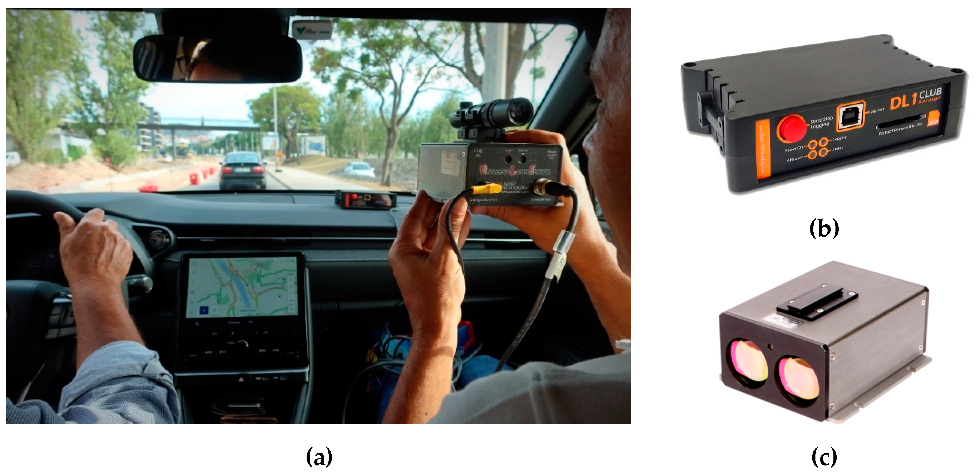
Figure 2.
Pilot study route.
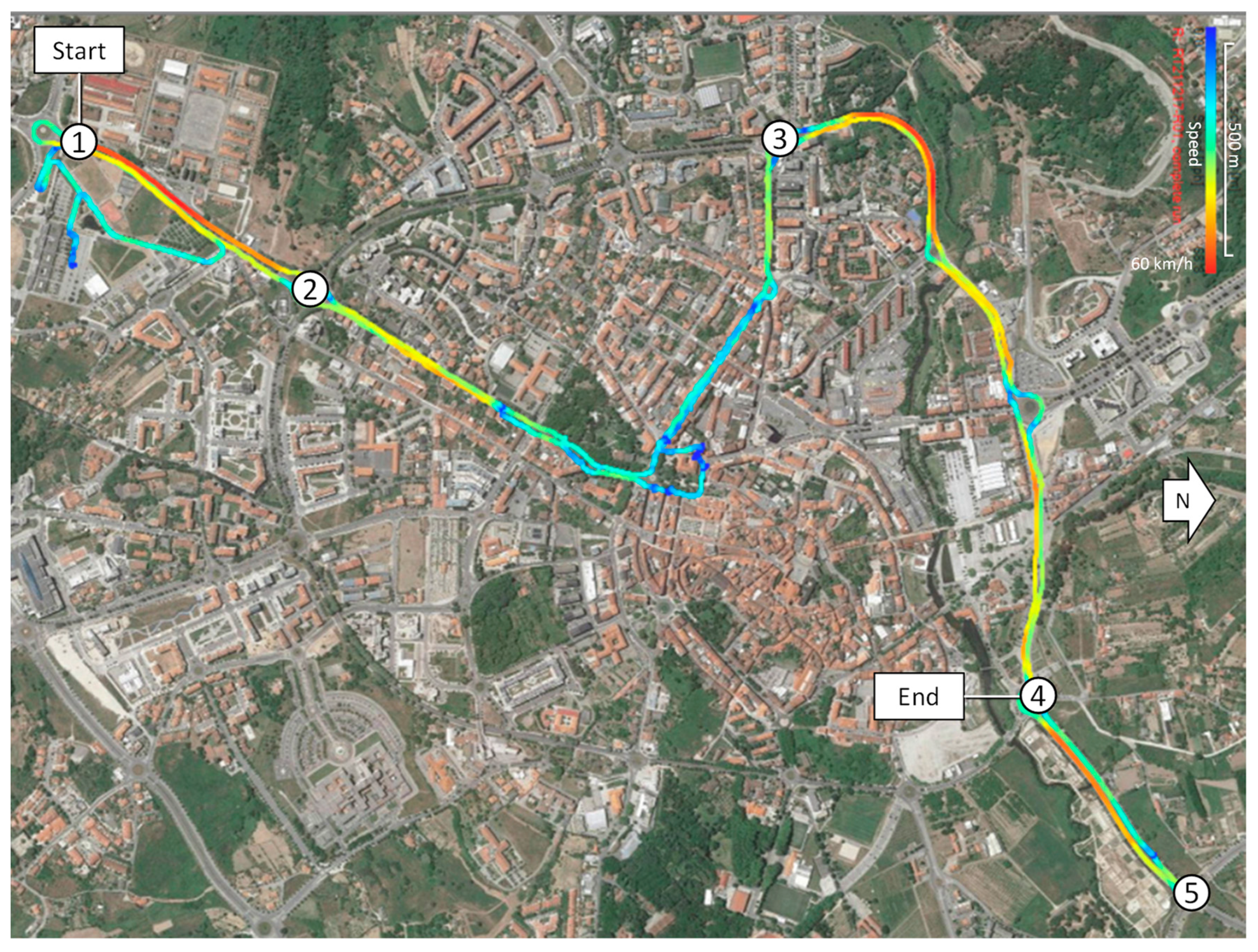
Figure 3.
Race Technology software: speed profile when crossing a roundabout (west → east direction).
Figure 3.
Race Technology software: speed profile when crossing a roundabout (west → east direction).
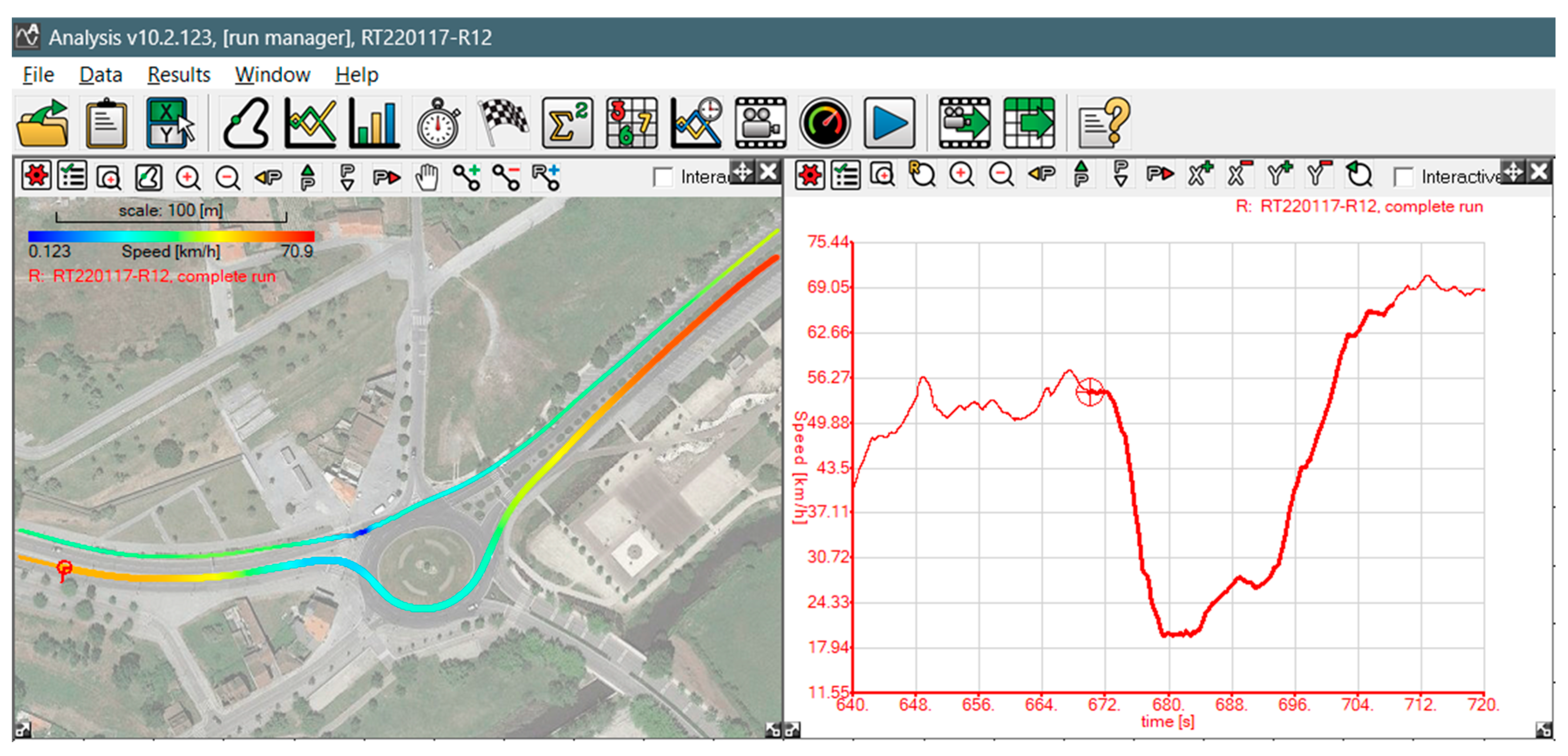
Figure 4.
Regression lines for v-s point data under steady-state conditions.
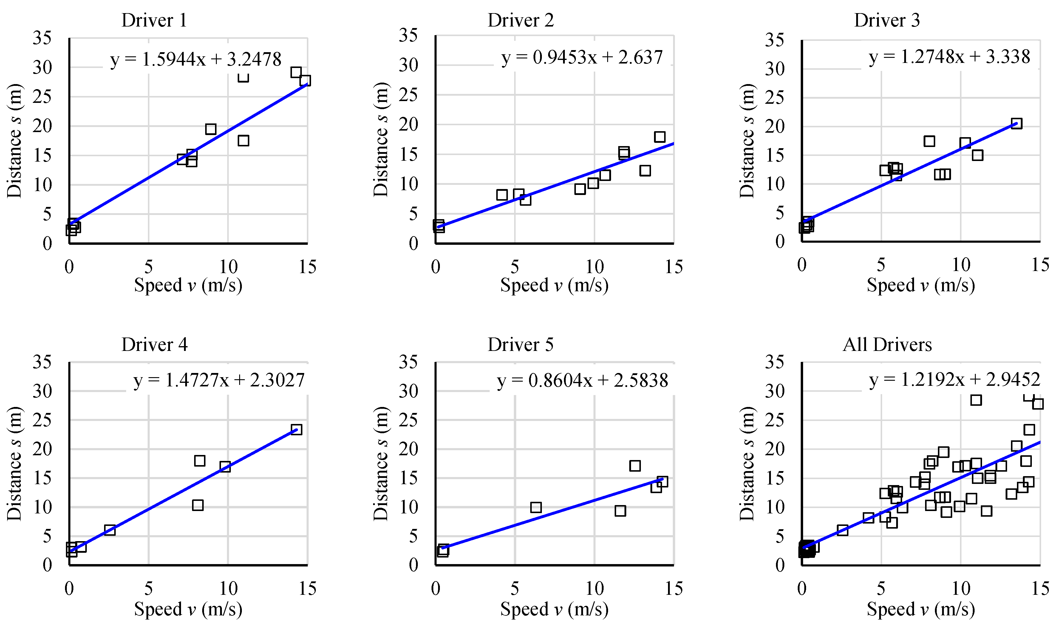
Figure 5.
Examples of kinematic profiles (observed vs. predicted by the IDM) for the acceleration maneuver under free-flow conditions. Left panel / right panel: vehicle with automatic / manual transmission.
Figure 5.
Examples of kinematic profiles (observed vs. predicted by the IDM) for the acceleration maneuver under free-flow conditions. Left panel / right panel: vehicle with automatic / manual transmission.
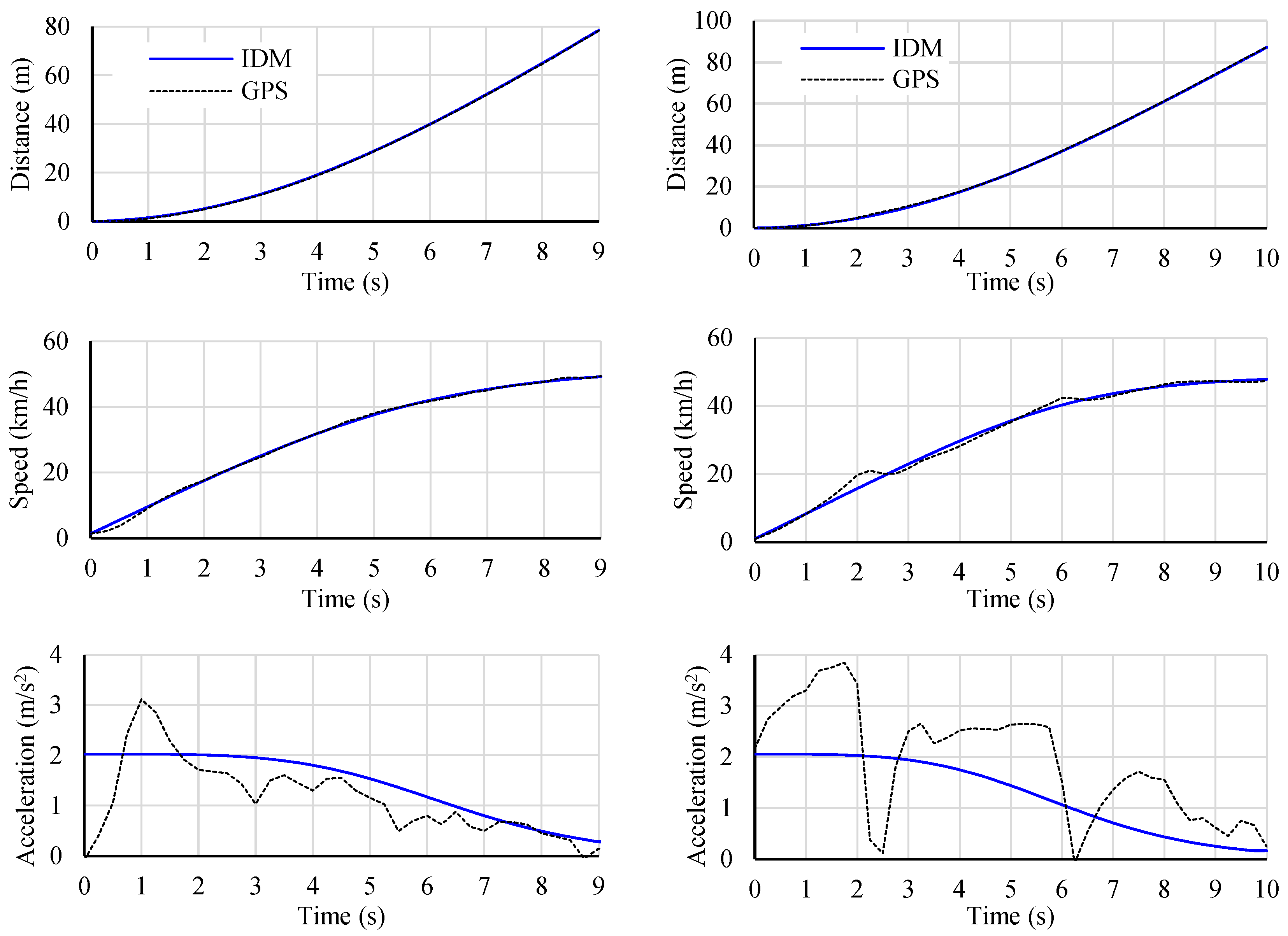
Figure 6.
Examples of kinematic profiles (observed vs IDM) for deceleration maneuvers under free-flow conditions.
Figure 6.
Examples of kinematic profiles (observed vs IDM) for deceleration maneuvers under free-flow conditions.
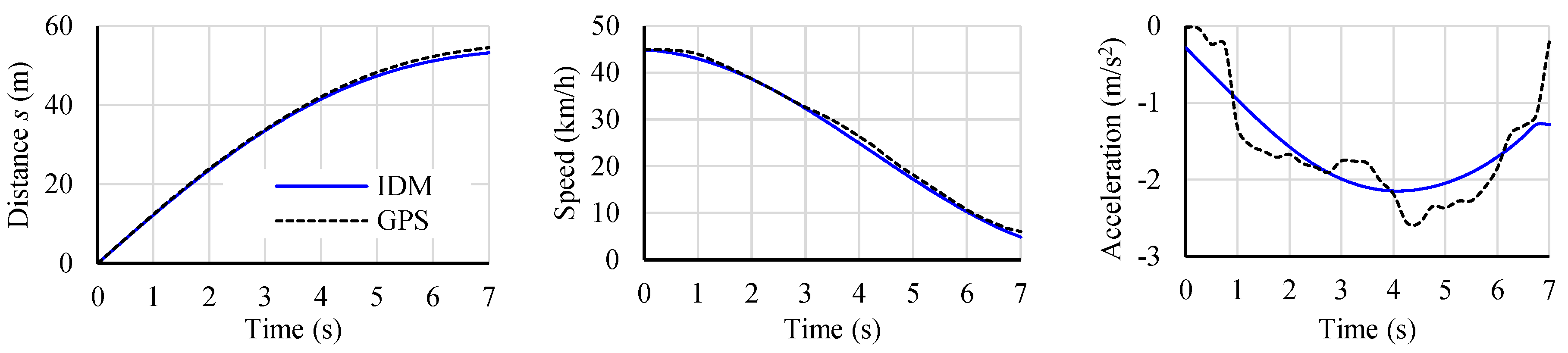
Figure 7.
Field vs. predicted speed profiles for drivers #1 and #2 during validation runs, using parameters calibrated for the opposite driving direction.
Figure 7.
Field vs. predicted speed profiles for drivers #1 and #2 during validation runs, using parameters calibrated for the opposite driving direction.
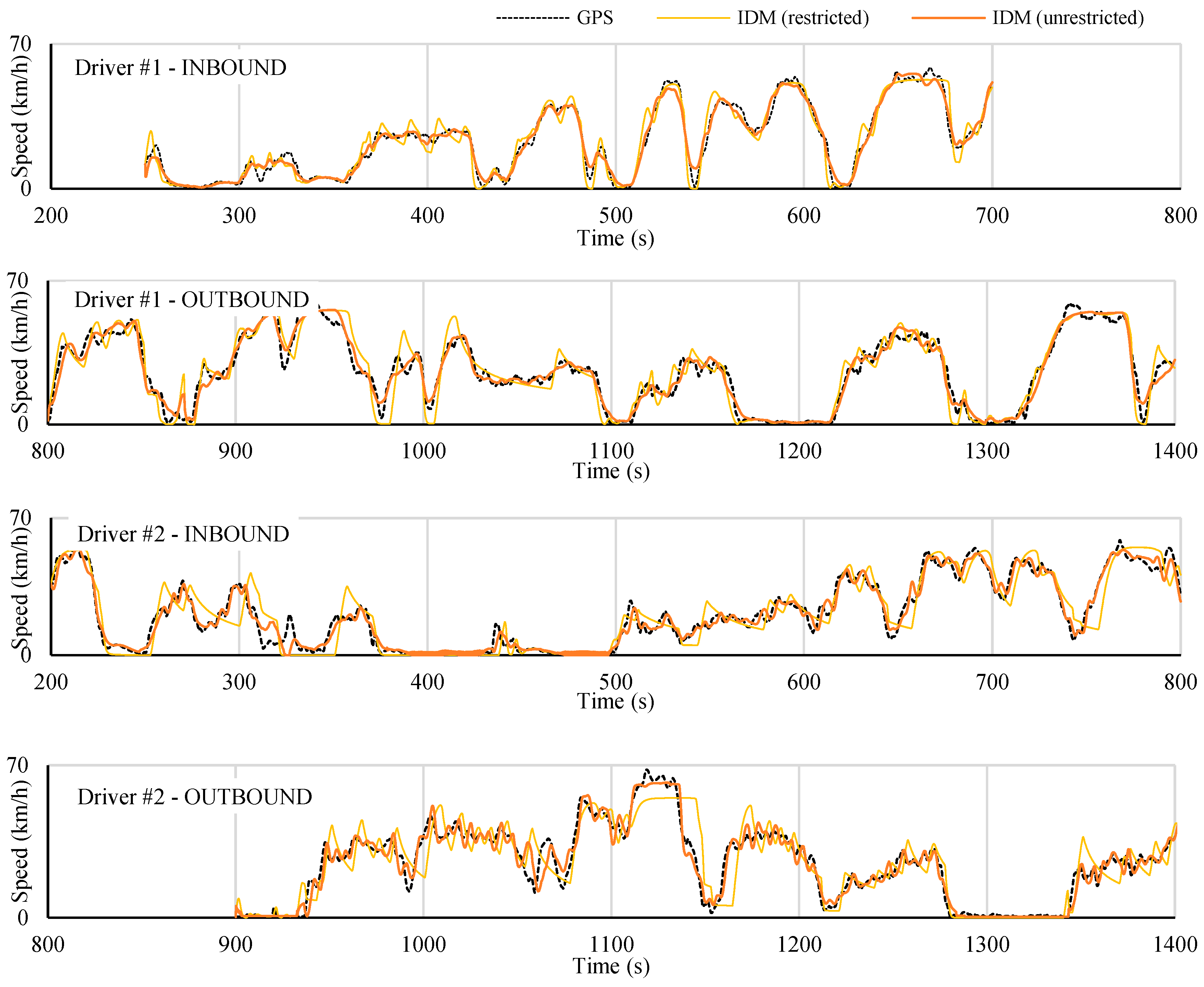

Table 1.
Parameter domain for the simultaneous estimation procedure: A – average, LB – lower bound, UB – upper bound.
Table 1.
Parameter domain for the simultaneous estimation procedure: A – average, LB – lower bound, UB – upper bound.
| Driver 1 | Driver 2 | Driver 3 | Driver 4 | Driver 5 | All | ||||||||||||
|---|---|---|---|---|---|---|---|---|---|---|---|---|---|---|---|---|---|
| Param. | A | LB | UB | A | LB | UB | A | LB | UB | A | LB | UB | A | LB | UB | LB | UB |
| s0 (m) | 3.25 | 1.63 | 4.88 | 2.64 | 1.32 | 3.96 | 3.34 | 1.67 | 5.01 | 2.30 | 1.15 | 3.45 | 2.58 | 1.29 | 3.87 | 0.50 | 10.00 |
| T (s) | 1.59 | 0.80 | 2.39 | 0.95 | 0.48 | 1.43 | 1.28 | 0.64 | 1.92 | 1.47 | 0.74 | 2.21 | 0.86 | 0.43 | 1.29 | 0.25 | 4.00 |
| a (m/s2) | 1.82 | 1.11 | 2.44 | 2.02 | 1.23 | 2.71 | 2.05 | 1.24 | 2.75 | 1.31 | 0.80 | 1.76 | 2.04 | 1.24 | 2.74 | 0.50 | 9.00 |
| b (m/s2) | 5.93 | 3.18 | 8.33 | 2.26 | 1.21 | 3.17 | 3.12 | 1.67 | 4.38 | 1.06 | 0.57 | 1.49 | 1.87 | 1.00 | 2.63 | 0.50 | 9.00 |
| δ | 3.42 | 2.11 | 4.86 | 2.40 | 1.48 | 3.41 | 1.13 | 0.70 | 1.61 | 4.78 | 2.95 | 6.79 | 5.80 | 3.58 | 8.24 | 0.50 | 10.00 |
Table 2.
Results of the calibration and cross-validation.
| Segment | Optimal parametrs (calibration segment) | RMSE | ||||||||||
|---|---|---|---|---|---|---|---|---|---|---|---|---|
| Driver | Mode | Calib. | Valid. | a | b | δ | T | s0 | Calib. | Valid. | ||
| #1 | Constrained | Out. | In. | 2.27 | 5.91 | 3.58 | 1.79 | 3.74 | 1.19 | 1.64 | ||
| In. | Out. | 2.37 | 7.17 | 3.10 | 1.88 | 3.96 | 1.58 | 1.21 | ||||
| Unconstrained | Out. | In. | 4.20 | 8.00 | 1.00 | 3.09 | 6.78 | 0.69 | 1.04 | |||
| In. | Out. | 7.95 | 7.97 | 2.42 | 3.00 | 9.50 | 0.96 | 0.75 | ||||
| #2 | Constrained | Out. | In. | 2.52 | 1.89 | 2.53 | 0.73 | 2.27 | 1.88 | 2.18 | ||
| In. | Out. | 2.08 | 2.42 | 2.52 | 1.25 | 3.63 | 2.13 | 2.00 | ||||
| Unconstrained | Out. | In. | 7.81 | 5.35 | 3.94 | 2.94 | 3.63 | 0.92 | 1.16 | |||
| In. | Out. | 7.95 | 7.52 | 3.31 | 2.96 | 4.73 | 1.12 | 0.95 | ||||
Disclaimer/Publisher’s Note: The statements, opinions and data contained in all publications are solely those of the individual author(s) and contributor(s) and not of MDPI and/or the editor(s). MDPI and/or the editor(s) disclaim responsibility for any injury to people or property resulting from any ideas, methods, instructions or products referred to in the content. |
© 2025 by the authors. Licensee MDPI, Basel, Switzerland. This article is an open access article distributed under the terms and conditions of the Creative Commons Attribution (CC BY) license (http://creativecommons.org/licenses/by/4.0/).
Copyright: This open access article is published under a Creative Commons CC BY 4.0 license, which permit the free download, distribution, and reuse, provided that the author and preprint are cited in any reuse.


