
Submitted:
06 January 2025
Posted:
07 January 2025
Read the latest preprint version here
Abstract
One of the main consequences of urban pollution is intersection congestion, which occurs due to frequent vehicle stops. These interruptions lead to increased fuel consumption and greenhouse gas emissions (CO2), along with other pollutants such as nitrogen oxides (NOX) and fine particulates. These pollutants can adversely affect the respiratory, cardiac, and neurological health of city residents. To address the growing demand for smart and sustainable transportation systems in large cities, predicting intersection congestion using artificial intelligence offers a promising solution. In this study, we present a predictive modeling approach to classify congestion levels at intersections controlled by traffic lights. Using the CN+ dataset collected in Bremen, Germany, our methodology incorporates vehicle and environmental features to predict congestion levels, optimize traffic flow, and reduce pollutant emissions. We employ data preprocessing, feature engineering, and machine learning techniques, including an innovative feature selection method called Dual Importance Intersection Feature Selection (DIFS), which combines Random Forest (RF) and Chi-square analysis. We tested various classifiers, including RF, XGBoost, LightGBM, CatBoost, and Artificial Neural Network (ANN), utilizing SMOTE balancing to address the class imbalance. Performance metrics such as precision, recall, F1 score, overall accuracy, and Quadratic Weighted Kappa (QWK) demonstrate promising results, with F1 and QWK scores reaching 100%. This makes our approach a robust tool for managing traffic sustainably and efficiently.
Keywords:
intersection congestion
; sustainable urban traffic
; artificial intelligence
; machine learning
; dual importance intersection feature selection
; emission reduction
; traffic flow optimization
1. Introduction
Urban traffic congestion, especially at intersections, represents a major challenge for sustainable urban development. Frequent vehicles stopping at traffic lights contributes significantly to increased fuel consumption and greenhouse gas emissions (GHG), including (), as well as harmful pollutants such as nitrogen oxides () and particulate matter (PM2.5). According to the World Health Organization (WHO), these pollutants contribute significantly to respiratory, cardiovascular, and neurological health problems and led to the premature deaths of 4.2 million people worldwide in 2019 [1]. Furthermore, the environmental impact of transport-related emissions has raised concerns worldwide and highlights the need for innovative solutions to alleviate congestion and its associated impacts [2,3,4,5].
To address these challenges, intelligent transportation systems (ITS) have emerged as a promising approach to optimize traffic management and reduce environmental impacts. ITS leverages data-driven technologies and artificial intelligence (AI) to improve traffic flow and decrease emissions, making them essential for transitioning to green and sustainable cities [6]. Among the key components of ITS is the ability to predict traffic congestion levels accurately at intersections. Predictive models facilitate proactive traffic light management, reducing idle time, minimizing delays, and lowering pollutant emissions [7]. However, the development of such models poses challenges, including handling imbalanced datasets, incorporating real-time data, and achieving high predictive performance [8].
Existing research has explored machine learning techniques for traffic congestion prediction, such as Random Forest (RF), Support Vector Machines (SVM), and Gradient Boosting (GB) [9,10,11]. While these studies have demonstrated the potential of machine learning in traffic management, many do not fully address the dynamic nature of urban traffic conditions. Furthermore, few studies combine real-time vehicle and environmental data to optimize urban transportation comprehensively.
This study uses the CN+ dataset gathered in Bremen, Germany, to suggest a novel predictive modeling approach to fill these gaps. This dataset contains extensive features on traffic and environmental conditions and enables a comprehensive analysis of intersection congestion. Our methodology introduces an innovative feature selection technique called DIFS, which integrates random forest and chi-square analysis to identify the most influential predictors. We use state-of-the-art machine learning models based on XGBoost, LightGBM, Random Forest, CatBoost, and ANN to classify congestion levels. Our results show significant improvements in prediction performance, with metrics such as precision, recall, F1-score, and QWK indicating high model reliability.
1.0.0.1. Novelty and contributions of the research:
This research makes several important contributions to sustainable urban transport management. First, it leverages DIFS for feature selection, providing a robust approach to identifying the most meaningful predictors of congestion. Second, integrating vehicle counts and environmental data into the modeling process increases the practical applicability of our approach. Third, by using ensemble machine learning models, high prediction accuracy is achieved, with F1 and QWK values reaching 100%. These contributions represent our work as an important step toward developing data-driven tools to reduce traffic congestion at intersections and promote green urban mobility.
The remainder of this paper is organized as follows: Section 2 reviews the literature on congestion prediction and sustainable traffic management. Section 3 describes the CN+ dataset and the preprocessing steps. Section 4 describes the methodology and machine learning techniques used. Section 5 presents the experimental results and discusses their implications. Finally, Section 6 concludes the study and suggests directions for future research.
2. Literature Review
In recent years, predictive modeling of traffic congestion has gained significant attention due to the increasing demands for sustainable urban mobility and efficient traffic management systems. Machine learning (ML) and deep learning (DL) methods have emerged as powerful tools for addressing congestion challenges at intersections.
Nematichari, A. et al. introduced a graph theory and trajectory data mining-based system that utilizes structural time series models to forecast intersection traffic conditions [12]. Their work provides real-time analytics and proactive decision-making capabilities, advancing urban traffic management. Similarly, Qin, Kun. et al. proposed a multiple-graph-based convolutional network (mGCN) integrating environmental data from street imagery and road networks to predict urban congestion spots with 85.5% accuracy, showcasing the importance of spatial correlations in urban environments [13].
Hybrid models have demonstrated significant potential in addressing traffic flow complexities. Olayode, I. O. et al. evaluated Adaptive Neuro-Fuzzy Inference Systems (ANFIS) and its Genetic Algorithm-optimized variant (ANFIS-GA) for predicting vehicular flow at intersections, achieving an R of 0.9980 with ANFIS-GA [14]. Moumen, Idriss. et al. applied Gated Recurrent Units (GRUs) to model temporal dependencies in multi-intersection traffic, highlighting the model’s robustness in handling sparse datasets [15].
Deep learning has further enhanced congestion prediction capabilities. Katambire, Vienna N. et al. demonstrated that LSTM networks outperform traditional ARIMA models for traffic flow forecasting at urban intersections [16]. Similarly, Mirzahossein, Hamid. et al. combined wavelet transforms with GRU-LSTM architectures, achieving over 94% accuracy in traffic volume prediction despite noisy data [17].
Hybridized techniques integrating machine learning and optimization algorithms have advanced congestion modeling. Chahal, Ayushi. et al. presented a SARIMA and Bi-LSTM hybrid model, achieving low error metrics for time-series traffic predictions [18]. Chaoura, Chaimaa. et al. employed LSTMs and Particle Swarm Optimization (PSO) to improve prediction accuracy, addressing noisy and dynamic traffic data challenges [19].
Innovative frameworks have also emerged for real-time traffic management. Wang, Jianlong. et al. introduced a Spatio-Temporal Neural Point Process (STNPP) model combining Graph Neural Networks and temporal dependencies to predict lane-level congestion events [20]. Gwalani, Aryan. et al. proposed an intelligent intersection framework incorporating GRUs and V2I communication for adaptive signal control, significantly reducing congestion and travel times [21].
Bayesian models and ensemble approaches have shown promise in enhancing traffic forecasting. AlKheder, Sharaf, et al. developed a Bayesian Combined Neural Network (BCNN) for short-term traffic volume prediction, achieving over 98% regression accuracy [22]. Navarro-Espinoza, Alfonso. et al. compared ML and DL methods, finding that MLP outperformed GRU and LSTM in traffic prediction for multi-lane intersections [23].
Studies by Giraka, Omkar. et al. [24] and Qu, Wenrui. et al. [25] have explored traditional time-series models such as SARIMA and two-layer stacking techniques for forecasting urban traffic. These methods provide scalable and computationally efficient solutions for heterogeneous urban environments.
Addressing limited historical data, Tsalikidis, Nikolaos. et al. employed LightGBM and Histogram-Based Gradient Boosted Regressor (HGBR), outperforming LSTMs and GRUs for IoT-enabled congestion management [26]. Tran, Quang Hoc, et al. adapted LSTM networks for multi-lane arterial roads in Vietnam, achieving superior accuracy with minimal infrastructure requirements [27]. Tang, Bin. et al. proposed a Directed Supra-Adjacency Matrix (DSAM) model for intersection ranking, leveraging Chebyshev networks to capture temporal dynamics [28].
Table 1 briefly summarizes the previous studies based on their focus, models evaluated, and key findings.
2.0.0.2. Analysis of Comparative Studies:
While existing studies have explored a range of machine learning and deep learning techniques for traffic congestion prediction, our work distinguishes itself in several ways. First, we leverage the CN+ dataset, which includes detailed vehicle and environmental features, enabling a more granular analysis of intersection congestion. Second, our approach integrates a novel feature selection technique, DIFS, combining RF and Chi-square methods to enhance model performance. Third, we achieve perfect F1 and QWK scores across multiple classifiers, including RF, XGBoost, LightGBM, CatBoost, and ANN, underscoring the robustness of our predictive framework.
3. Dataset Description
This section provides an overview of the dataset used in this paper. First, we describe the data source origin, followed by a detailed explanation of the dataset’s attributes and relevance.
3.1. Origin of the Dataset
This research leverages the CN+ dataset [29], a valuable resource for studies in ITS and Vehicular Ad-hoc Networks (VANETs). The dataset was collected over 32 hours at a four-way signalized intersection in Bremen, Germany, between May 24 and August 6, 2022. Due to privacy concerns regarding video-based collection methods, the authors used a manual write-down procedure for the data collection.
The dataset captures a comprehensive range of traffic conditions, including morning and evening rush hours, peak and off-peak periods, and variations in traffic density between weekdays and weekends. The CN+ dataset includes 25,935 vehicles, along with additional features such as weather conditions, significantly enhancing the dataset’s applicability for modeling and simulation.
The CN+ dataset is publicly hosted on the Zenodo platform and distributed under a Creative Commons Attribution License (CC BY 4.0). This accessibility encourages its use in a wide array of research applications. By focusing on an intersection with mixed traffic types—including private vehicles, public transport, and trams—the dataset provides a robust foundation for developing and evaluating predictive algorithms for congestion management and vehicular safety systems. Figure 1 illustrates the intersection in Bremen, Germany, where the dataset was collected.
3.2. Data Description
The CN+ dataset originally contained 15,022 rows and 12 attributes. However, by using feature engineering to extract additional attributes and applying the DIFS approach for feature selection, we end up with 13 attributes as input parameters for the prediction model. For more details about the feature engineering process and DIFS approach, see the methodology section of this paper. The final attributes used as input parameters for the prediction models are as follows:
- Number: The number of vehicles in a group (cluster);
- Direction: Direction taken by the vehicle (14 possible directions, numbered 1 to 14);
- Second: The time of collection in seconds, extracted from the Date column;
- Type: Type of vehicle (Normal, Bus, Tram);
- Weekday: Day of the week;
- Day: Day of the month;
- Temperature: Ambient temperature (e.g., 61°F);
- Humidity: Humidity level;
- Hour: Hour of the day;
- IsWeekend: Attribute indicating whether it is a weekend day;
- Atmospheric pressure (e.g., 29.71 in);
- Wind Speed: Wind gusts speed;
- Month: Month of the year.
The Congestion_Level attribute represents the target variable. This attribute categorizes congestion into three levels: low, medium, and high. Figure 2 below shows the distribution of the different categories of the target variable.
Analysis of Figure 2 above shows an imbalance problem in the dataset. Therefore, it is imperative to adopt a data-balancing strategy to prevent a drop in performance of the predictive models from deteriorating. This issue will be addressed in the methodology section of our article.
4. Methodology
In this section, we describe the methodological approach to develop a predictive model for intersection congestion detection based on the CN+ dataset. The problem was formulated as a multiclass classification task, where each congestion category corresponded to a specific severity level: low, medium, and high. This categorization of congestion severity forms the basis of the predictive modeling framework for solving the multiclass prediction problem.
Our methodological approach includes evaluating and comparing the performance of several machine learning algorithms: RF, XGBoost, LightGBM, CatBoost, and ANN. These algorithms were selected to predict intersection congestion levels with high confidence, focusing on model generalization and performance. The main goal is to highlight the best algorithm in this study context.
In the remainder of this section, we provide a detailed description of the steps taken to develop our predictive models for intersection congestion detection using the CN+ dataset. We outline the development environment, highlight the data preprocessing approach, and explain the feature engineering process, exploratory data analysis, predictive model construction, and validation and evaluation phases. The ultimate goal is to establish an intersection congestion detection system to improve traffic flow control, reduce harmful gas emissions from frequent vehicle stops, and facilitate the transition of major cities worldwide to greener, more environmentally sustainable urban ecosystems.
4.1. Development Environment
The development environment used in this study is similar to the one described in the article published by Muktar, B. et al. [11]. For further details, please refer to Section 4.1 of the referenced publication.
4.2. Data Preprocessing
In this subsection, we describe the key preprocessing techniques used to prepare the CN+ dataset for predictive modeling. These measures improved model performance, guaranteed data quality, and resolved data compatibility issues with machine learning algorithms.
4.2.1. Temporal Data Consolidation
The data set initially contained two separate columns for date (in YYYY.MM.DD format) and time (in HH:MM:SS format). To optimize the analysis, these columns were merged into a single Datetime column using the to_datetime function from the Pandas library. The original Date and Time columns were then removed. This consolidation enabled the extraction of additional temporal features such as day of the week, hour, and minute for further analysis.
4.2.2. Weather-Related Attributes Conversion
The Temperature and Dew Point columns contained values with the unit °F. To convert these columns to numeric values, the °F unit was removed, and the values were converted to float32. Similarly, the same process was applied to the Humidity, Wind Speed, Wind Gust, and Pressure columns by removing their respective units (% for Humidity, mph for Wind Speed and Wind Gust, and in for Pressure). Table 2 and Table 3 below provide examples of the values from these columns before and after the transformations.
4.2.3. Direction Encoding
The Direction column, which specified vehicular directions (e.g., "Direction 13"), was preprocessed by removing the string prefix and converting the values to integers. This transformation ensured compatibility with machine learning models.
4.2.4. Conversion of Wind Directions to Degrees
The Wind Direction column was converted into corresponding angular values in degrees using a custom mapping (e.g., North = 0°, East = 90°). This preprocessing step facilitated the numerical analysis of directional data, enabling its integration into predictive models. Figure 3 below illustrates this transformation.
4.2.5. Encoding Categorical Variables
Categorical attributes, such as Type (Normal, Bus, Tram, and Bike), were encoded numerically using a manual mapping strategy. For example:
- Normal vehicles were assigned a value of 0;
- Buses were encoded as 1, trams as 2, and bikes as 3.
4.3. Handling Missing Values
The Datetime column contained 12 missing entries (0.08% of the dataset). These records were removed as their impact on the dataset was negligible. Following this, the dataset was verified to be free of missing values.
4.4. Feature Engineering
To enhance the dataset, additional attributes were derived from the consolidated Datetime column to capture temporal patterns with greater precision:
- Weekday: Day of the week, represented numerically (0–6);
- Day: Day of the year;
- Month: Month of the year;
- Year: Year of the observation;
- IsWeekend: Binary indicator for weekends, where 1 represents a weekend, and 0 represents a weekday;
- Hour, Minute, and Second: Extracted to provide finer temporal granularity.
These engineered features provide valuable insights into traffic patterns, facilitating more effective predictive modeling and significantly contributing to the accuracy and interpretability of the models.
4.5. Assigning Congestion Levels
Congestion levels were assigned to each record based on the Number attribute, which represents the count of vehicles crossing the intersection simultaneously. This approach enables the classification of congestion severity into three levels: Low, Medium, and High.
To define these levels, percentile thresholds were calculated from the Number distribution. Specifically, the 33rd and 66th percentiles were used as cutoffs to segment the data into three ranges. Records with Number values less than or equal to the 33rd percentile were classified as Low Congestion, those between the 33rd and 66th percentiles were labeled as Medium Congestion, and values exceeding the 66th percentile were designated as High Congestion. This percentile-based classification ensures a systematic and data-driven segmentation of congestion levels.
The assignment was automated using a mapping function that compared each record’s Number value against the calculated thresholds. This method ensured consistent classification of all records in the dataset. The resulting Congestion_Level attribute provides a categorical representation of congestion severity, serving as the target variable for predictive modeling.
4.6. Dual Importance Intersection Feature Selection (DIFS)
The Dual Importance Intersection Feature Selection (DIFS) approach combines two complementary feature selection methods, RF and Chi-Square (), to identify the most important features for predictive modeling. This hybrid approach leverages the strengths of both methods:
- RF evaluates the importance of each feature by measuring its contribution to reducing uncertainty within a decision tree model. This makes it well suited for capturing nonlinear relationships between features and the target variable;
- evaluates the statistical relationship between each feature and the target variable and prioritizes features that have strong relationships based on categorical data analysis.
The DIFS methodology selects the top 15 features identified by each method and uses their intersection to retain only the features deemed important by both approaches. This ensures the selection of robust and informative features while mitigating potential biases introduced by a single method.
4.6.0.1. Advantages of DIFS:
- Robustness: By using two distinct criteria—model contribution and statistical association—DIFS minimizes the risk of over-reliance on a single selection method, ensuring more reliable feature selection;
- Redundancy Reduction: By focusing on the intersection of the two methods, DIFS eliminates redundant or uninformative features, resulting in a leaner feature set that improves model performance and reduces overfitting;
- Improved Interpretability: The selected features are both statistically significant and impactful to the model, improving the interpretability of the resulting predictive model;
- Adaptability: DIFS can be customized to integrate other feature selection techniques, providing the flexibility to test different combinations of algorithms for various datasets and modeling needs.
In summary, DIFS provides a balanced and reliable feature selection framework and improves model performance by focusing on features that are both meaningful and non-redundant. This approach ensures the development of predictive models that are not only robust but also interpretable and efficient.
The Table 4 presents the feature importance scores and selection results obtained using the DIFS approach, which combines RF and statistical methods.
4.7. Data Balancing Using SMOTE
The training dataset had a significant class imbalance in the target variable Congestion_Level, with 5,794 records in the Low Congestion class, 1,630 in the Medium Congestion class, and 1,541 in the High Congestion class. Such imbalance can negatively impact the performance of machine learning models as they tend to favor the majority class, leading to biased predictions and poor generalization for underrepresented classes.
To address this problem, we used the Synthetic Minority Oversampling Technique (SMOTE) [31], a widely used algorithm for oversampling minority classes in imbalanced datasets. SMOTE generates synthetic samples for the minority classes instead of duplicating existing samples. These synthetic examples are created by interpolating between a sample and its nearest neighbors in feature space, preserving the diversity and variability of the dataset.
After applying SMOTE, the training dataset was balanced, with each class—Low, Medium, and High Congestion—containing 5,794 samples. This balancing ensures that the model is not biased toward the majority class, allowing it to learn the characteristics of all congestion levels effectively. By leveraging SMOTE, we aim to improve the robustness and generalization capability of the predictive model, especially for the minority classes, resulting in better overall performance.
4.8. Exploratory Data Analysis
Understanding the data distribution and identifying key patterns is essential for developing an effective predictive model for congestion levels at the traffic intersection. This section explores the dataset through various dimensions, including the relationship between vehicle counts, temporal trends, and directional traffic flows. The analysis highlights significant trends and correlations that will inform the modeling process.
4.8.1. Relationship Between Vehicle Count and Congestion Level
The violin plot presented in Figure 4 illustrates the relationship between the number of vehicles (Number) and congestion levels (Congestion_Level). The congestion levels are divided into three categories: Low, Medium, and High, with the number of vehicles represented on the y-axis.
Figure 4 highlights several important observations:
- Low and Medium Congestion Levels: For congestion levels categorized as Low and Medium, the number of vehicles is consistently low, predominantly concentrated around 1 or 2. This indicates that minimal vehicular presence corresponds to these lower congestion levels;
- High Congestion Level: For the High congestion level, the distribution of vehicle counts is much broader. The number of vehicles ranges significantly, with the density peak observed around 5. The spread and height of the distribution suggest that a larger number of vehicles is a key indicator of high congestion;
- Distribution Shape: The sharp increase in density for High congestion at lower vehicle counts, coupled with a long tail extending to higher counts, reflects the variability in vehicular presence during high congestion scenarios. This highlights the importance of accounting for such variability in predictive modeling.
This analysis demonstrates the strong correlation between the number of vehicles and congestion severity. Consequently, the feature Number is a critical predictor for modeling congestion levels at intersections.
4.8.2. Hourly Traffic Patterns
Figure 5 below shows the hourly distribution of congestion levels (low, medium, and high) over different times of the day and provides valuable insights into the traffic patterns at the intersection. Each bar represents the total number of congestion incidents recorded per hour, segmented by severity.
The previous plot reveals several key observations:
- Morning Traffic (8 AM - 10 AM): The number of congestion incidents steadily increases from 1,731 at 8 AM to 2,005 at 10 AM. This trend indicates increasing traffic flow during the morning rush hours, with a notable proportion of High and Medium severity levels;
- Afternoon Traffic (3 PM - 6 PM): Congestion incidents peak between 4 PM and 5 PM, reaching a maximum of 2,543 at 5 PM. This reflects the typical evening rush hour, where high congestion levels dominate, suggesting significant delays and traffic buildup;
- Severity Proportions: Throughout the day, Low congestion levels (green) form the main proportion of incidents, followed by Medium (yellow) and High (red). However, during peak hours, the proportion of High severity levels increases significantly, highlighting critical traffic management challenges.
Analysis of Figure 5 underscores the importance of time-specific traffic management strategies. The peak congestion hours identified in the graph can guide the deployment of interventions, such as adaptive traffic light control, to alleviate delays and enhance traffic flow. These insights are essential for developing predictive models tailored to address temporal variations in congestion.
4.8.3. Day of the Week vs. Congestion Level
Figure 6 illustrates the variation in congestion levels (low, medium, and high) on different weekdays and provides critical insights into weekly traffic patterns at the intersection.
Figure 6 reveals the following key observations :
-
Higher Congestion on Weekdays:
- -
- Congestion incidents are notably higher from Monday to Thursday, with Tuesday and Wednesday showing the peak total congestion levels at 2,508 and 2,491 incidents, respectively;
- -
- Low Congestion (green) dominates, followed by Medium (yellow) and High (red) congestion levels. The presence of High Congestion highlights the impact of weekday commuting patterns.
-
Reduced Congestion on Weekends:
- -
- A significant reduction in congestion incidents is observed on Saturday and Sunday, with totals dropping to 1,670 and 1,721 incidents, respectively. This aligns with lower traffic volumes typically associated with weekends;
- -
- Low congestion incidents continue to occur most frequently on these days, while high congestion incidents occur less frequently compared to weekdays.
-
Transition on Friday:
- -
- Friday marks a transition between the high congestion levels of weekdays and the lower congestion of weekends, with 1,973 total incidents. This reflects the changing traffic dynamics as work-related commuting gives way to leisure and weekend activities.
This analysis emphasizes the temporal variability in traffic patterns and congestion severity. Incorporating the Weekday feature into predictive models can enhance their accuracy by accounting for these observed trends, particularly the sharp contrast between weekdays and weekends. Targeted traffic management strategies for peak congestion days like Tuesday and Wednesday could further improve intersection efficiency.
4.8.4. Direction of Vehicles vs. Congestion Level
Figure 7 below shows the distribution of congestion levels (low, medium, and high) based on the direction of vehicle movement at the intersection. Each bar represents the total number of congestion events for a given direction, segmented by severity.
Figure 7 reveals key insights below:
-
Dominant Congestion Directions:
- -
- Directions 6 and 13 account for the highest number of congestion incidents, with totals of 6,242 and 5,792, respectively. These directions exhibit a substantial proportion of High Congestion (red) and Medium Congestion (yellow), indicating their critical role in overall traffic congestion at the intersection;
- -
- This dominance suggests that these directions may correspond to main traffic inflow or outflow routes.
-
Lower Congestion in Other Directions:
- -
- Directions 2, 9, 10, 11, and 12 have significantly fewer incidents, with totals ranging between 13 and 207. These directions show predominantly Low Congestion (green), implying less frequent or less severe traffic issues.
-
Intermediate Congestion Levels:
- -
- Directions such as 1, 3, 5, 7, and 8 show moderate numbers of congestion incidents, with a mix of Low and Medium congestion levels. This pattern may reflect secondary traffic routes or turning lanes with moderate traffic density.
-
Traffic Dynamics at Intersections:
- -
- The evident disparity in congestion levels across directions suggests directional bias in traffic flow, likely influenced by factors such as road hierarchy, intersection design, or traffic signal timing.
The analysis of Figure 7 highlights the importance of considering direction as a predictive feature when modeling at the congestion level. Targeted traffic management strategies such as optimizing traffic light times or adding dedicated lanes for high-volume directions could effectively ease congestion in critical directions such as 6 and 13. These insights are critical for developing a robust predictive model and improving traffic flow at intersections.
4.8.5. Monthly Traffic Trends
Figure 8 depicts the monthly distribution of congestion incidents (Low, Medium, and High) across four months: May, June, July, and August. Each bar represents the total number of congestion incidents recorded during a specific month, segmented by congestion severity levels.
Figure 8 above reveals the following critical insights:
-
Peak Congestion in May and July:
- -
- May records the highest total number of congestion incidents at 5,828, closely followed by July with 5,242 incidents. These months are dominated by Low Congestion (green), but both show a notable proportion of Medium (yellow) and High Congestion (red) levels. The high traffic volumes during these months may correspond to seasonal patterns or increased travel activity.
-
Drop in June and August:
- -
- June and August exhibit significantly lower congestion levels, with 2,492 and 1,460 total incidents, respectively. These months have smaller proportions of High Congestion incidents, indicating relatively smoother traffic flow during this period.
-
Severity Distribution:
- -
- Across all months, Low Congestion levels form the majority, followed by Medium and High Congestion. However, the share of High Congestion is more prominent in May and July, emphasizing the challenges of managing traffic during these peak months.
-
Temporal Variations:
- -
- The sharp contrast between months with high congestion (May and July) and those with lower congestion (June and August) highlights the importance of incorporating Month as a feature in predictive modeling. Understanding such temporal trends can significantly improve the model’s ability to anticipate congestion levels.
The previous analysis suggests that traffic management strategies should be tailored to account for monthly variations, particularly during high-congestion months like May and July. These insights are crucial for predictive models aiming to optimize traffic flow and reduce delays at the intersection considered in this study.
Keys Factors Influencing Congestion Level at the Intersection:
Based on the exploratory data analysis, several key factors influence congestion levels at the intersection:
- Number of Vehicles: A strong correlation is observed between the number of vehicles and congestion severity, with higher vehicle counts associated with high congestion levels.
- Time of Day: Morning and evening rush hours significantly impact congestion levels, particularly during peak times (8-10 AM and 4-6 PM).
- Day of the Week: Weekdays experience higher congestion levels compared to weekends, driven by weekday commuting patterns.
- Direction of Vehicles: Traffic flow patterns, particularly from dominant directions such as 6 and 13, heavily influence congestion.
- Monthly Variations: Seasonal changes and monthly variations, as observed in May and July, highlight the importance of accounting for temporal trends in predictive modeling.
The previous insights could serve as a foundation for building predictive models and inform targeted strategies to mitigate congestion at intersections.
4.9. Development of the Predictive Model
This subsection describes the methodological approach to implementing a predictive model for classifying the congestion level at intersections. To achieve this, we compared the performance of several classification algorithms, including RF, XGBoost, LightGBM, CatBoost and, ANN. We chose to base predictive modeling on these algorithms because numerous studies in the literature highlight their effectiveness on classification problems in the context of ITS [11,32,33,34].
To effectively evaluate the performance of these algorithms, we used an 80-20 data partitioning strategy, where 80% of the data is used for training and 20% for testing. It is generally accepted in the literature that this approach provides an optimal balance between the data required for training and the data reserved for testing. However, in our study, the first 20% of the dataset from the first split is reserved exclusively for simulating model performance in a real environment. The reserved 20% of data points are never seen by the model during the training phase. We then performed a secondary 80-20 partitioning of the remaining 80% of the dataset, with 80% dedicated to training and 20% dedicated to internal testing.
The evaluation and comparison of the classification algorithms were based on metrics such as accuracy, recall, precision, F1 score, and Quadratic Weighted Kappa. This approach aims to identify the classification algorithm that offers the best trade-off between prediction performance and generalization ability.
Our methodology ensures that the selected algorithm not only performs well on the training data but also maintains high reliability in real-world applications, making it a crucial part of effective traffic management systems at intersections.
5. Results and Discussion
This section outlines the performance outcomes of the machine learning models employed and provides an in-depth analysis of the findings.
5.1. Results
5.2. Discussion
The performance metrics presented in Table 5 and Figure 9 reveal consistent results across all evaluated models: RF, XGBoost, LightGBM, CatBoost, and ANN. Each model achieved perfect scores for performance metrics such as precision, recall, F1 score, accuracy, and QWK, showcasing their excellent predictive capabilities in classifying congestion levels (Low, Medium, High) at intersections.
Ensemble methods like XGBoost and LightGBM excelled in managing complex datasets, providing precise predictions across all classes while achieving high QWK scores that minimize misclassifications. RF and CatBoost showed admirable performance with identical metrics, demonstrating robustness and generalization. The ANN also performed well, effectively modeling nonlinear relationships.
Figure 9 illustrates the uniformity of the model performances, attributed to efficient preprocessing steps like data balancing and feature engineering, which ensured high-quality input features.
Despite equal performance, real-world applicability may differ. XGBoost and LightGBM are ideal for scenarios needing explainability and efficiency, while ANN may be suited for more complex patterns but could require high computational resources.
In summary, while all models performed exceptionally, the choice of the optimal algorithm will depend on specific requirements, such as computational efficiency, scalability, or interpretability. The insights from this analysis lay a strong groundwork for future improvements in predictive congestion management systems.
6. Conclusions and Future Research
In this study, we proposed a predictive modeling framework to assess congestion levels at intersections, leveraging machine learning techniques to address critical challenges in urban traffic management. Using the CN+ dataset collected in Bremen, Germany, our approach integrated data preprocessing, innovative feature selection using the DIFS method, and the application of robust machine learning algorithms such as RF, XGBoost, LightGBM, CatBoost, and ANN. The results showed exceptional prediction accuracy across all models, with perfect precision, recall, F1 scores, and QWK metrics.
The findings highlight the significant role of features such as vehicle count, temporal trends (hourly and weekly patterns), traffic direction, and monthly variations in influencing congestion levels. These insights provide a comprehensive understanding of congestion dynamics and support the development of targeted traffic management strategies, such as adaptive traffic signal control and optimized lane configurations.
This research contributes to the growing knowledge of sustainable urban traffic management by offering a scalable and efficient methodology for real-time congestion prediction. The integration of real-world vehicle and environmental data further enhances the practical applicability of the proposed models, promoting a transition toward greener and more sustainable urban ecosystems.
Based on the robust results obtained in this study, future research can focus on several key areas to expand the scope and applicability of the proposed framework:
- Geographic Scalability: Extending the predictive framework to diverse urban environments, including intersections with varying traffic patterns and road configurations, can validate its generalizability and adaptability.
- Enhanced Feature Engineering: Exploring additional predictive features, such as traffic incidents, weather anomalies, or pedestrian flow, could refine model performance and offer deeper insights into congestion causality.
- Interactive Decision Support Systems: Developing user-friendly interfaces for traffic management authorities, integrating real-time predictions, and visualizing congestion hotspots can facilitate proactive decision-making and resource allocation.
- Integration with Emission Control Strategies: Combining congestion prediction with models for estimating vehicular emissions can enable comprehensive approaches to mitigating traffic delays and environmental impacts.
By addressing the future directions above, the proposed framework can evolve into a versatile tool for intelligent transportation systems, contributing significantly to the realization of sustainable and efficient urban traffic networks.
Author Contributions
Conceptualization, B.M.; Methodology, B.M. and V.F.; Software, B.M.; Investigation, B.M.; Writing—original draft, Bappa Muktar; Writing—review & editing, V.F and N.A. All authors have read and agreed to the published version of the manuscript.
Funding
This research received no external funding.
Data Availability Statement
The dataset used in this study is available on the Zenodo website at https://doi.org/10.5281/zenodo.8189767 under the attribution license (CC-BY 4.0), accessed on 19 November 2024.
Conflicts of Interest
The authors declare no conflicts of interest.
References
- World Health Organization. Ambient (outdoor) air pollution. https://www.who.int/news-room/fact-sheets/detail/ambient-(outdoor)-air-quality-and-health, 2024. Accessed: 2024-12-10.
- Minderytė, A.; Pauraite, J.; Dudoitis, V.; Plauškaitė, K.; Kilikevičius, A.; Matijošius, J.; Rimkus, A.; Kilikevičienė, K.; Vainorius, D.; Byčenkienė, S. Carbonaceous aerosol source apportionment and assessment of transport-related pollution. Atmospheric Environment 2022, 279, 119043. [Google Scholar] [CrossRef]
- Li, J.; Wang, C.; Abdoli, S.; Yuen, A.C.; Kook, S.; Yeoh, G.H.; Chan, Q.N. Economic burden of transport related pollution in Australia. Journal of Transport & Health 2024, 34, 101747. [Google Scholar]
- Bajwa, A.U.; Sheikh, H.A. Contribution of road transport to Pakistan’s air pollution in the urban environment. Air 2023, 1, 237–257. [Google Scholar] [CrossRef]
- Pietrzak, K.; Pietrzak, O. Environmental effects of electromobility in a sustainable urban public transport. Sustainability 2020, 12, 1052. [Google Scholar] [CrossRef]
- Balta, M.; Özcelik, I. Traffic signaling optimization for intelligent and green transportation in smart cities. In Proceedings of the 2018 3rd International conference on computer science and engineering (UBMK). IEEE; 2018; pp. 31–35. [Google Scholar]
- Shahid, N.; Shah, M.A.; Khan, A.; Maple, C.; Jeon, G. Towards greener smart cities and road traffic forecasting using air pollution data. Sustainable Cities and Society 2021, 72, 103062. [Google Scholar] [CrossRef]
- Zhong, H.; Chen, K.; Liu, C.; Zhu, M.; Ke, R. Models for predicting vehicle emissions: A comprehensive review. Science of the Total Environment, 2024; 171324. [Google Scholar]
- Yang, J.; Han, S.; Chen, Y. Prediction of traffic accident severity based on random forest. Journal of Advanced Transportation 2023, 2023, 7641472. [Google Scholar] [CrossRef]
- Zhong, W.; Du, L. Predicting Traffic Casualties Using Support Vector Machines with Heuristic Algorithms: A Study Based on Collision Data of Urban Roads. Sustainability 2023, 15, 2944. [Google Scholar] [CrossRef]
- Muktar, B.; Fono, V. Toward Safer Roads: Predicting the Severity of Traffic Accidents in Montreal Using Machine Learning. Electronics 2024, 13, 3036. [Google Scholar] [CrossRef]
- Nematichari, A.; Pechlivanoglou, T.; Papagelis, M. Evaluating and forecasting the operational performance of road intersections. In Proceedings of the Proceedings of the 30th International Conference on Advances in Geographic Information Systems, 2022; pp. 1–12.
- Qin, K.; Xu, Y.; Kang, C.; Kwan, M.P. A graph convolutional network model for evaluating potential congestion spots based on local urban built environments. Transactions in GIS 2020, 24, 1382–1401. [Google Scholar] [CrossRef]
- Olayode, I.O.; Tartibu, L.K.; Alex, F.J. Comparative study analysis of ANFIS and ANFIS-GA models on flow of vehicles at road Intersections. Applied Sciences 2023, 13, 744. [Google Scholar] [CrossRef]
- Moumen, I.; Mahdaoui, R.; Raji, F.Z.; Rafalia, N.; Abouchabaka, J. Distributed Multi-Intersection Traffic Flow Prediction using Deep Learning. In Proceedings of the E3S Web of Conferences. EDP Sciences, Vol. 477; 2024; p. 00049. [Google Scholar]
- Katambire, V.N.; Musabe, R.; Uwitonze, A.; Mukanyiligira, D. Forecasting the Traffic Flow by Using ARIMA and LSTM Models: Case of Muhima Junction. Forecasting 2023, 5, 616–628. [Google Scholar] [CrossRef]
- Mirzahossein, H.; Gholampour, I.; Sajadi, S.R.; Zamani, A.H. A hybrid deep and machine learning model for short-term traffic volume forecasting of adjacent intersections. IET Intelligent Transport Systems 2022, 16, 1648–1663. [Google Scholar] [CrossRef]
- Chahal, A.; Gulia, P.; Gill, N.S.; Priyadarshini, I. A hybrid univariate traffic congestion prediction model for IOT-enabled smart city. Information 2023, 14, 268. [Google Scholar] [CrossRef]
- CHAOURA, C.; LAZAR, H.; JARIR, Z. Traffic Flow Prediction at Intersections: Enhancing with a Hybrid LSTM-PSO Approach. International Journal of Advanced Computer Science & Applications 2024, 15. [Google Scholar]
- Wang, J.; Duan, X.; Wang, P.; Qiu, A.G.; Chen, Z. Predicting urban signal-controlled intersection congestion events using spatio-temporal neural point process. International Journal of Digital Earth 2024, 17, 2376270. [Google Scholar] [CrossRef]
- Gwalani, A.; Pai, A.; Padalia, A.; Bhavathankar, P.; Devadkar, K. Prediction and Management of Traffic Congestion in Urban Environments. In Proceedings of the 2024 15th International Conference on Computing Communication and Networking Technologies (ICCCNT). IEEE; 2024; pp. 1–6. [Google Scholar]
- AlKheder, S.; Alkhamees, W.; Almutairi, R.; Alkhedher, M. Bayesian combined neural network for traffic volume short-term forecasting at adjacent intersections. Neural Computing and Applications 2021, 33, 1785–1836. [Google Scholar] [CrossRef]
- Navarro-Espinoza, A.; López-Bonilla, O.R.; García-Guerrero, E.E.; Tlelo-Cuautle, E.; López-Mancilla, D.; Hernández-Mejía, C.; Inzunza-González, E. Traffic flow prediction for smart traffic lights using machine learning algorithms. Technologies 2022, 10, 5. [Google Scholar] [CrossRef]
- Giraka, O.; Selvaraj, V.K. Short-term prediction of intersection turning volume using seasonal ARIMA model. Transportation letters 2020, 12, 483–490. [Google Scholar] [CrossRef]
- Qu, W.; Li, J.; Yang, L.; Li, D.; Liu, S.; Zhao, Q.; Qi, Y. Short-term intersection traffic flow forecasting. Sustainability 2020, 12, 8158. [Google Scholar] [CrossRef]
- Tsalikidis, N.; Mystakidis, A.; Koukaras, P.; Ivaškevičius, M.; Morkūnaitė, L.; Ioannidis, D.; Fokaides, P.A.; Tjortjis, C.; Tzovaras, D. Urban traffic congestion prediction: a multi-step approach utilizing sensor data and weather information. Smart Cities 2024, 7, 233–253. [Google Scholar] [CrossRef]
- Tran, Q.H.; Fang, Y.M.; Chou, T.Y.; Hoang, T.V.; Wang, C.T.; Vu, V.T.; Ho, T.L.H.; Le, Q.; Chen, M.H. Short-term traffic speed forecasting model for a parallel multi-lane arterial road using GPS-monitored data based on deep learning approach. Sustainability 2022, 14, 6351. [Google Scholar] [CrossRef]
- Tang, B.; Hu, Y. Frequent congestion detection model based on critical intersection identification. Transportation research record 2023, 2677, 371–385. [Google Scholar] [CrossRef]
- Karunathilake, Thenuka and Zongo, Meyo and Amarawardana, Dinithi and Förster, Anna. CN+: Vehicular Dataset at Traffic Light Regulated Intersection in Bremen, Germany. Zenodo, 2023. [Online; accessed ]. 19 November 2024.
- Karunathilake, T.; Zongo, M.; Amarawardana, D.; Förster, A. CN+: Vehicular Dataset at Traffic Light Regulated Intersection in Bremen, Germany. Scientific Data 2024, 11, 665. [Google Scholar] [CrossRef] [PubMed]
- Chawla, N.V.; Bowyer, K.W.; Hall, L.O.; Kegelmeyer, W.P. SMOTE: synthetic minority over-sampling technique. Journal of artificial intelligence research 2002, 16, 321–357. [Google Scholar] [CrossRef]
- Hassan, M.A.; Salem, H.; Bailek, N.; Kisi, O. Random forest ensemble-based predictions of on-road vehicular emissions and fuel consumption in developing urban areas. Sustainability 2023, 15, 1503. [Google Scholar] [CrossRef]
- Park, J.; Hwang, E. A two-stage multistep-ahead electricity load forecasting scheme based on LightGBM and attention-BiLSTM. Sensors 2021, 21, 7697. [Google Scholar] [CrossRef]
- Chahal, A.; Gulia, P.; Gill, N.S.; Priyadarshini, I. A hybrid univariate traffic congestion prediction model for IOT-enabled smart city. Information 2023, 14, 268. [Google Scholar] [CrossRef]
Figure 1.
Aerial view of the intersection where the dataset was collected [30].
Figure 1.
Aerial view of the intersection where the dataset was collected [30].
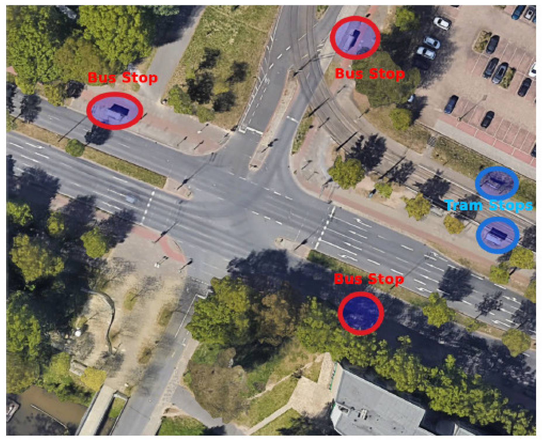
Figure 2.
Distribution of Congestion Levels.
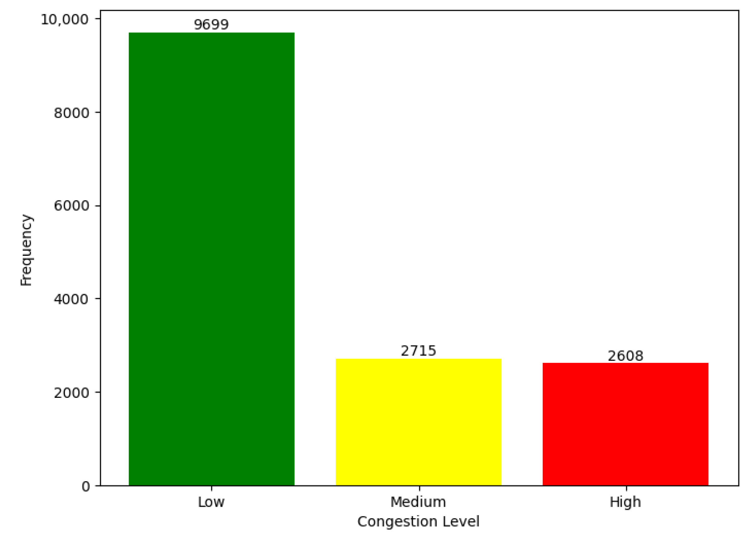
Figure 3.
Wind Direction Mapping to Degrees.
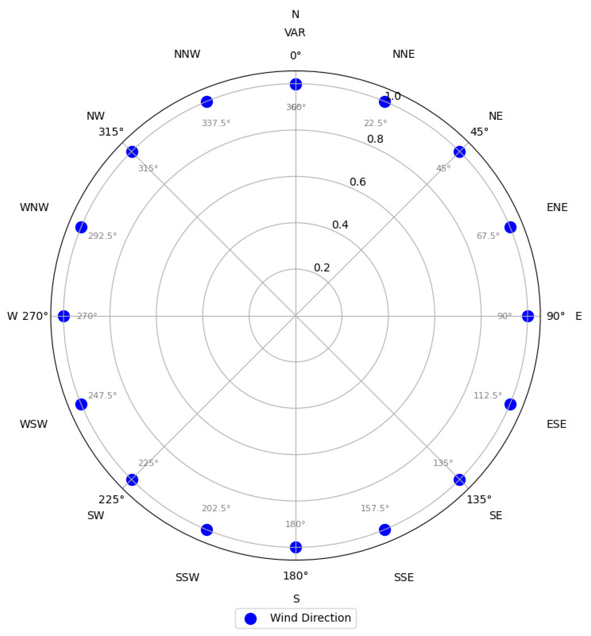
Figure 4.
Relationship Between Vehicle Count and Congestion Level.
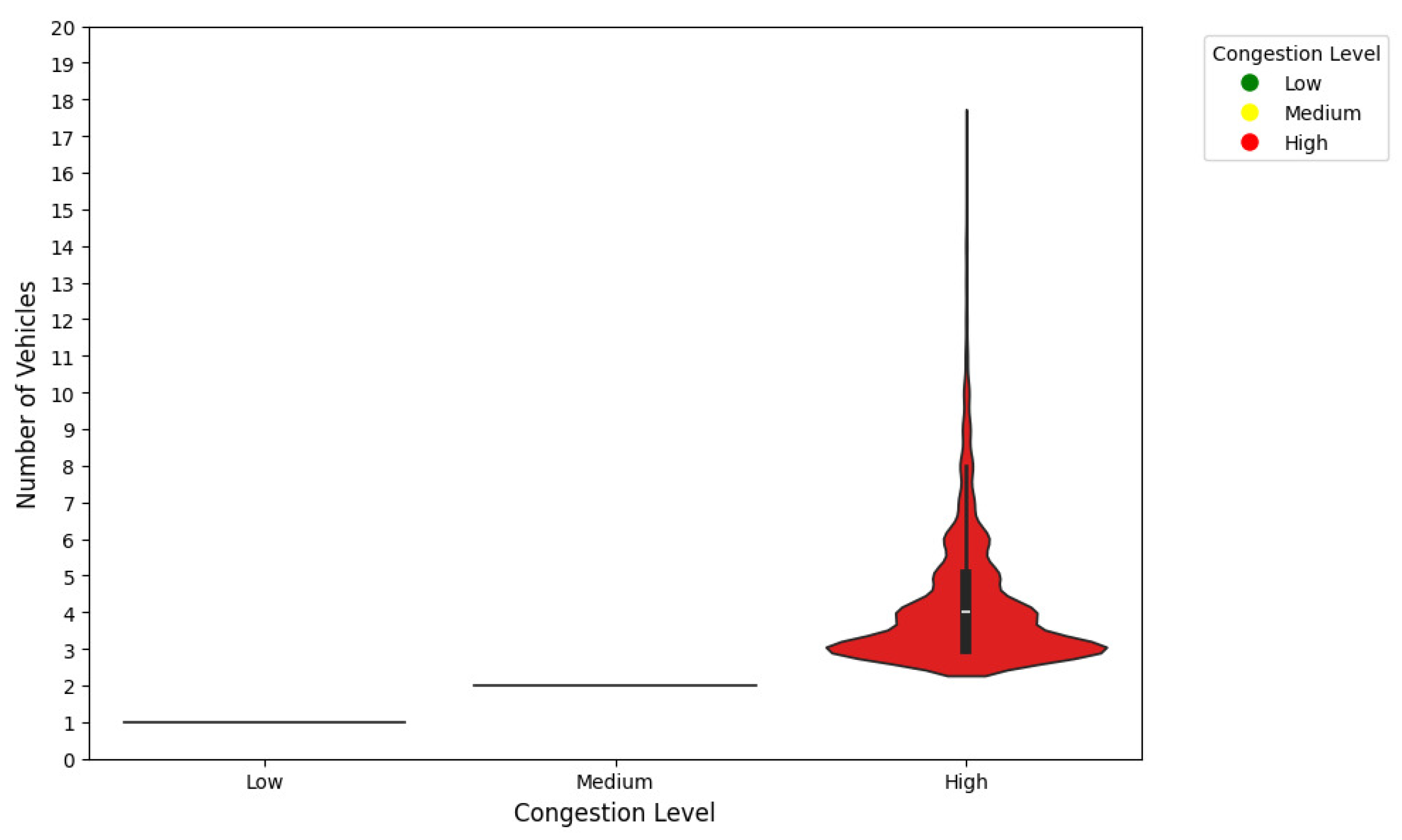
Figure 5.
Hourly Variations in Congestion Incidents.
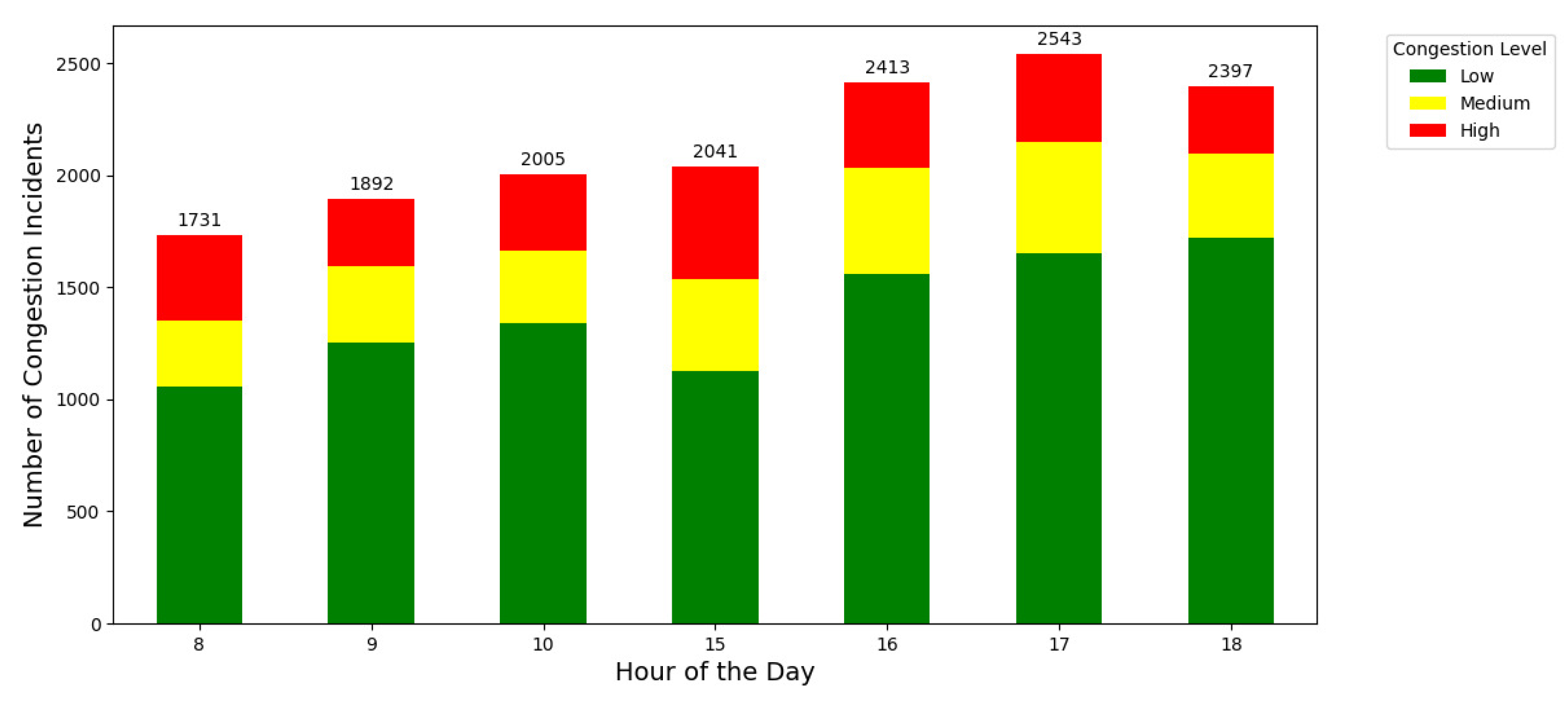
Figure 6.
Weekly Distribution of Congestion Incidents.
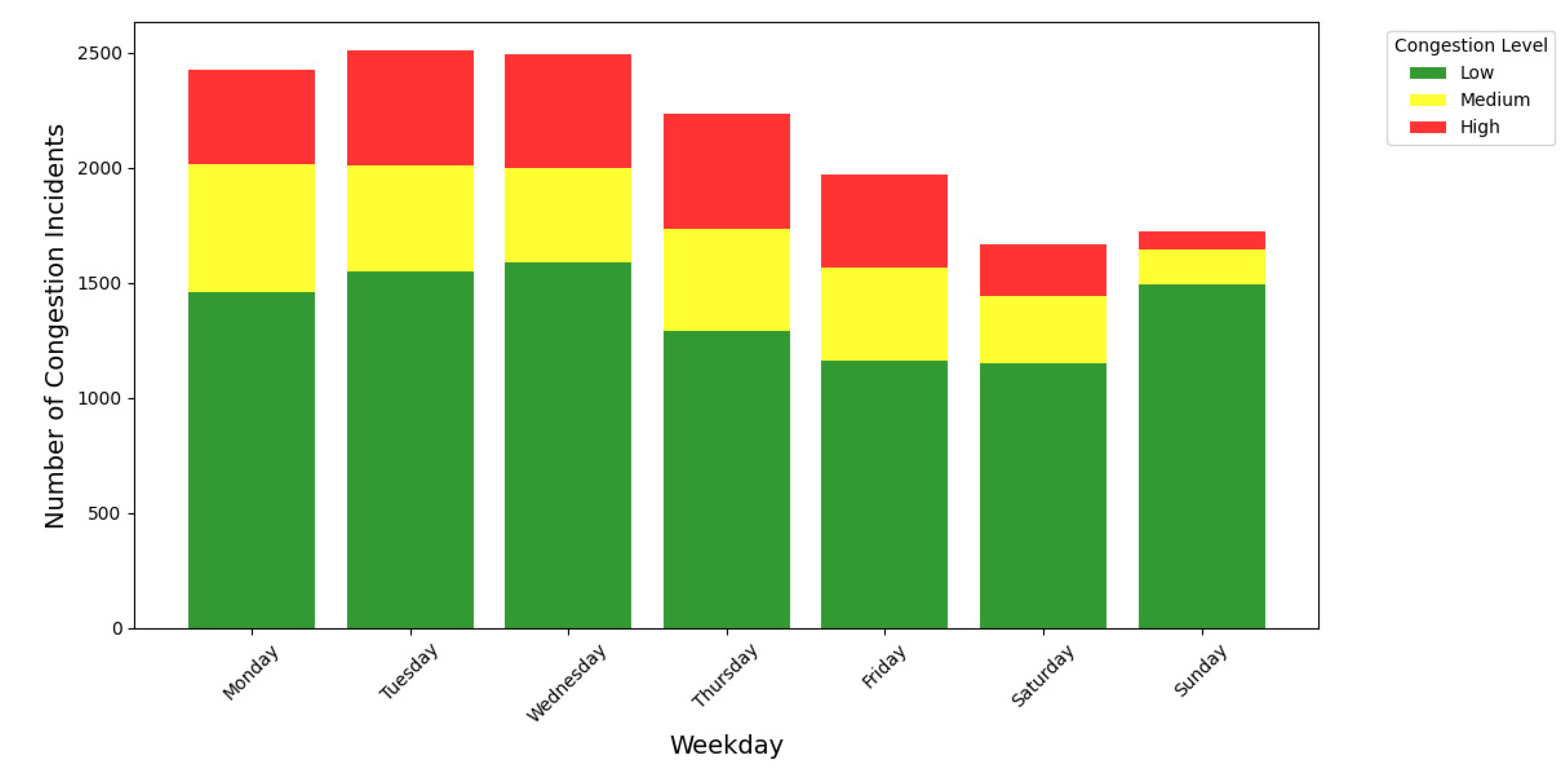
Figure 7.
Direction of Vehicles vs. Congestion Level.
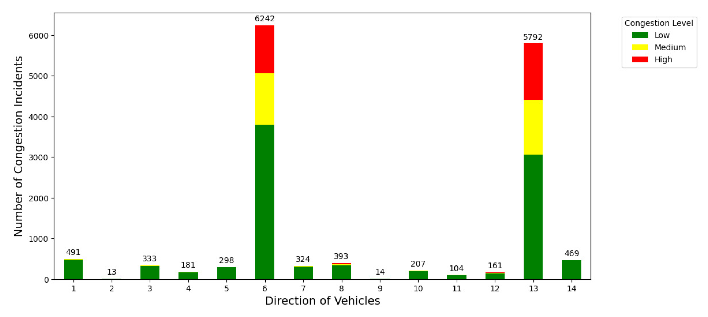
Figure 8.
Monthly Variations in Congestion Incidents.
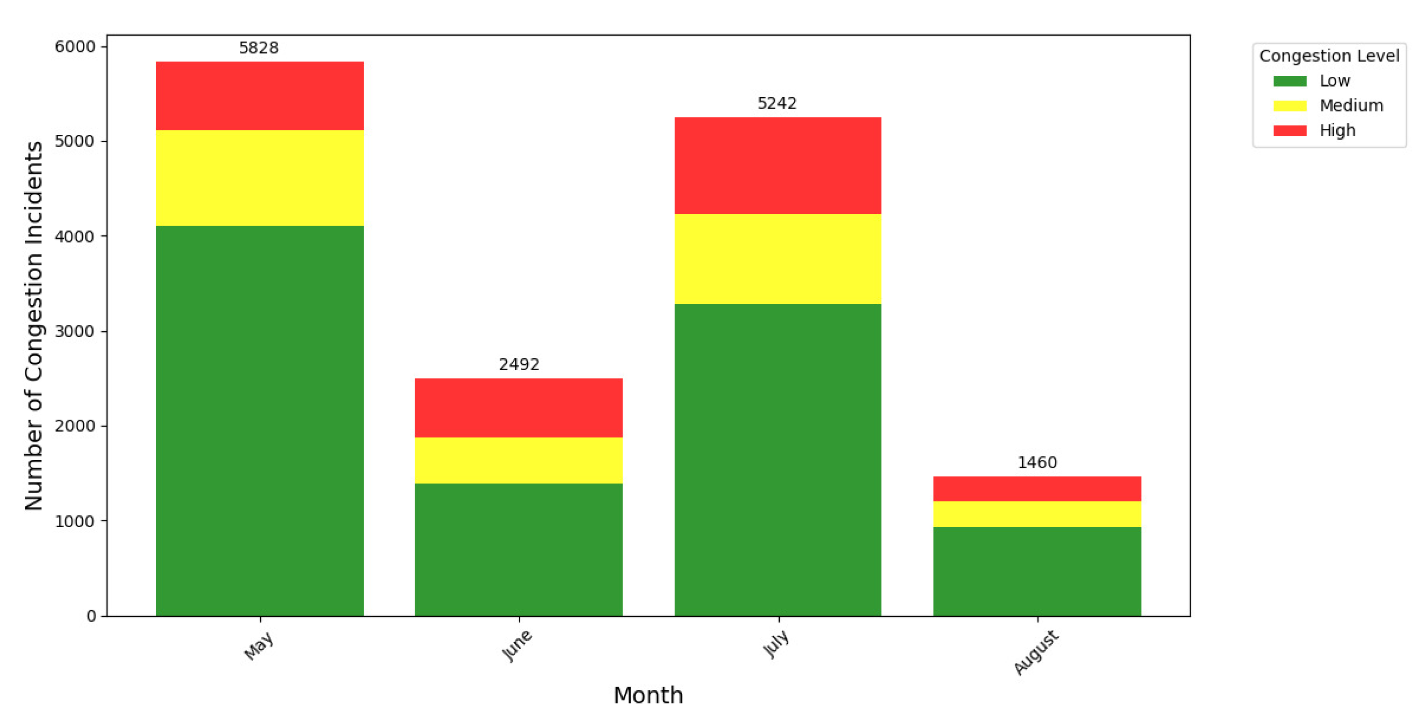
Figure 9.
Comparison of classification algorithm performance.
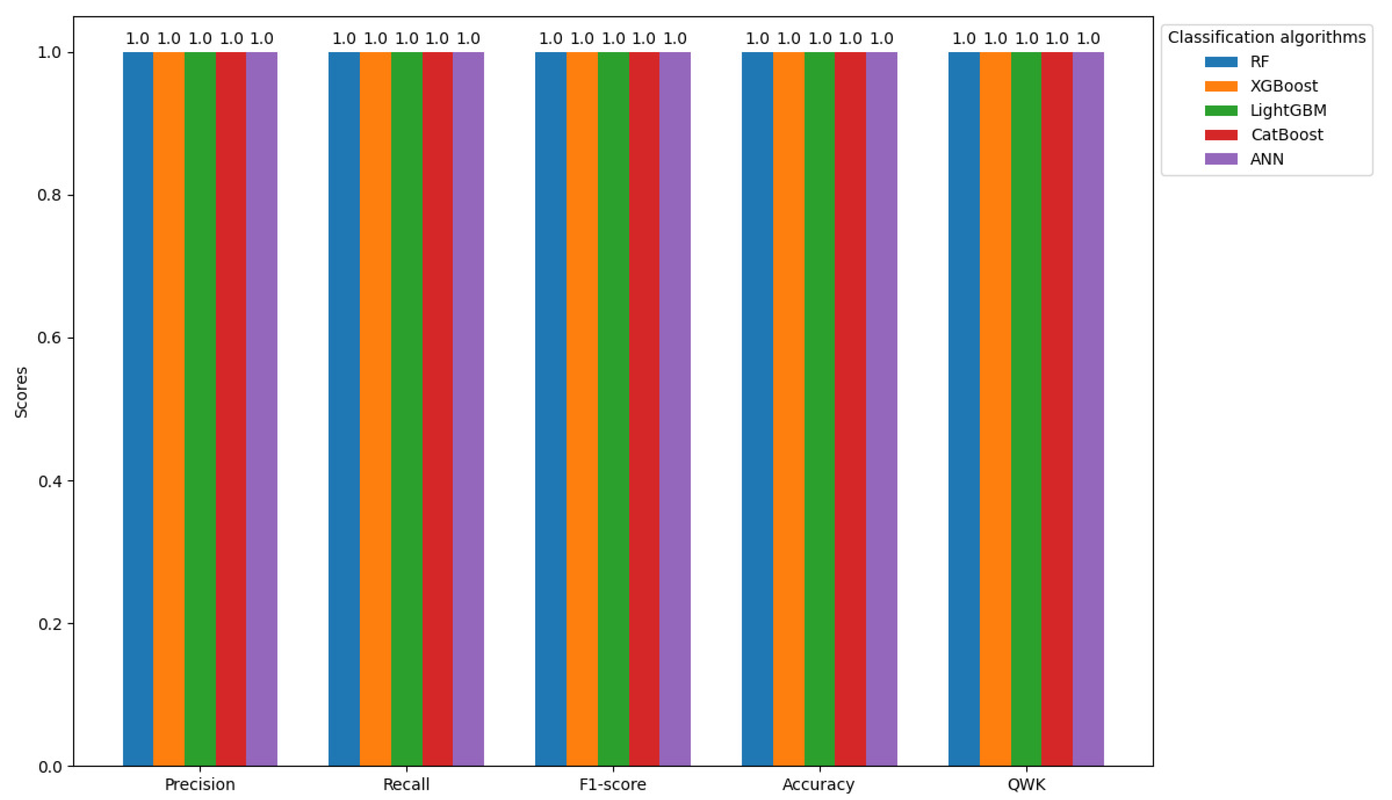

Table 1.
Comparative analysis of machine learning approaches for predicting congestion levels at intersections.
Table 1.
Comparative analysis of machine learning approaches for predicting congestion levels at intersections.
| Reference | Focus | Models/Techniques | Key Findings |
|---|---|---|---|
| [12] | Intersection traffic forecasting | Graph theory, trajectory mining | Real-time analytics with structural time series models. |
| [13] | Urban congestion spot identification | mGCN, DenseNet | Achieved 85.5% accuracy in predicting congestion spots. |
| [14] | Traffic flow prediction | ANFIS, ANFIS-GA | ANFIS-GA achieved R² = 0.9980, surpassing standalone ANFIS. |
| [15] | Multi-intersection traffic modeling | GRU | Demonstrated robust performance even with sparse datasets. |
| [16] | Traffic flow forecasting | LSTM, ARIMA | LSTM outperformed ARIMA in predictive reliability. |
| [17] | Volume prediction | GRU-LSTM, wavelet transform | Achieved 94% accuracy through hybrid noise reduction methods. |
| [18,19] | Hybrid modeling | SARIMA + Bi-LSTM, LSTM + PSO | Achieved low RMSE and high prediction accuracy across test cases. |
| [20,21] | Real-time management frameworks | STNPP, GRU + V2I communication | Effective in reducing congestion and optimizing travel times. |
| [22,23] | Bayesian and ensemble approaches | BCNN, MLP | High regression accuracy; robust multi-lane intersection predictions. |
| [24,25] | Time-series and stacking methods | SARIMA, KNN + Elman NN | Offered computationally efficient and scalable solutions. |
| [26,27,28] | IoT and directed networks | LightGBM, DSAM, LSTM | Reliable congestion management for urban planning and traffic optimization. |
| Current Work | Congestion level prediction at intersections | RF, XGBoost, LightGBM, CatBoost, ANN | Achieved perfect F1 and QWK scores using CN+ dataset with advanced feature selection (DIFS). |
Table 2.
Sample values of weather-related attributes before transformation.
| Temperature | Dew Point | Humidity | Wind Speed | Wind Gust | Pressure |
|---|---|---|---|---|---|
| 61 °F | 48 °F | 63 % | 15 mph | 0 mph | 29.71 in |
| 61 °F | 48 °F | 63 % | 15 mph | 0 mph | 29.71 in |
| 61 °F | 48 °F | 63 % | 15 mph | 0 mph | 29.71 in |
| 61 °F | 48 °F | 63 % | 15 mph | 0 mph | 29.71 in |
| 61 °F | 48 °F | 63 % | 15 mph | 0 mph | 29.71 in |
Table 3.
Sample values of weather-related attributes after transformation.
| Temperature | Dew Point | Humidity | Wind Speed | Wind Gust | Pressure |
|---|---|---|---|---|---|
| 61.0 | 48.0 | 63.0 | 15.0 | 0.0 | 29.71 |
| 61.0 | 48.0 | 63.0 | 15.0 | 0.0 | 29.71 |
| 61.0 | 48.0 | 63.0 | 15.0 | 0.0 | 29.71 |
| 61.0 | 48.0 | 63.0 | 15.0 | 0.0 | 29.71 |
| 61.0 | 48.0 | 63.0 | 15.0 | 0.0 | 29.71 |
Table 4.
Feature importance scores and selection results from the Dual DIFS method.
| Feature | Importance (RF) | Score () | Top 15 RF | Top 15 | Selected (Final Features) |
|---|---|---|---|---|---|
| Number | 0.900267 | 1418.054207 | True | True | True |
| Direction | 0.018842 | 33.116457 | True | True | True |
| Second | 0.014737 | 2.197631 | True | True | True |
| Type | 0.012121 | 256.689034 | True | True | True |
| Weekday | 0.006432 | 38.393137 | True | True | True |
| Day | 0.005297 | 21.434902 | True | True | True |
| Temperature | 0.005136 | 16.758210 | True | True | True |
| Humidity | 0.004894 | 13.497951 | True | True | True |
| Hour | 0.003438 | 4.778054 | True | True | True |
| IsWeekend | 0.003056 | 228.424129 | True | True | True |
| Pressure | 0.002675 | 7.180566 | True | True | True |
| Wind Speed | 0.002200 | 3.593028 | True | True | True |
| Month | 0.001966 | 20.931367 | True | True | True |
| Minute | 0.001442 | 0.617892 | True | False | False |
| Dew Point | 0.002470 | 0.950019 | True | False | False |
| Wind | 0.001823 | 2.148818 | False | False | False |
| Wind Gust | 0.000223 | 29.798063 | False | False | False |
* This table highlights the features selected by both RF and methods in the DIFS approach.
Table 5.
Summary of classification results across different models.
| Class | Precision | Recall | F1-score | Accuracy | QWK Score | Support |
|---|---|---|---|---|---|---|
| Random Forest (RF) | ||||||
| Low | 1.00 | 1.00 | 1.00 | - | - | 530 |
| Medium | 1.00 | 1.00 | 1.00 | - | - | 1925 |
| High | 1.00 | 1.00 | 1.00 | - | - | 536 |
| Overall | 1.00 | 1.00 | 1.00 | 1.00 | 1.00 | 2991 |
| XGBoost | ||||||
| Low | 1.00 | 1.00 | 1.00 | - | - | 530 |
| Medium | 1.00 | 1.00 | 1.00 | - | - | 1925 |
| High | 1.00 | 1.00 | 1.00 | - | - | 536 |
| Overall | 1.00 | 1.00 | 1.00 | 1.00 | 1.00 | 2991 |
| LightGBM | ||||||
| Low | 1.00 | 1.00 | 1.00 | - | - | 530 |
| Medium | 1.00 | 1.00 | 1.00 | - | - | 1925 |
| High | 1.00 | 1.00 | 1.00 | - | - | 536 |
| Overall | 1.00 | 1.00 | 1.00 | 1.00 | 1.00 | 2991 |
| CatBoost | ||||||
| Low | 1.00 | 1.00 | 1.00 | - | - | 530 |
| Medium | 1.00 | 1.00 | 1.00 | - | - | 1925 |
| High | 1.00 | 1.00 | 1.00 | - | - | 536 |
| Overall | 1.00 | 1.00 | 1.00 | 1.00 | 1.00 | 2991 |
| Artificial Neural Network (ANN) | ||||||
| Low | 1.00 | 1.00 | 1.00 | - | - | 530 |
| Medium | 1.00 | 1.00 | 1.00 | - | - | 1925 |
| High | 1.00 | 1.00 | 1.00 | - | - | 536 |
| Overall | 1.00 | 1.00 | 1.00 | 1.00 | 1.00 | 2991 |
Disclaimer/Publisher’s Note: The statements, opinions and data contained in all publications are solely those of the individual author(s) and contributor(s) and not of MDPI and/or the editor(s). MDPI and/or the editor(s) disclaim responsibility for any injury to people or property resulting from any ideas, methods, instructions or products referred to in the content. |
© 2025 by the authors. Licensee MDPI, Basel, Switzerland. This article is an open access article distributed under the terms and conditions of the Creative Commons Attribution (CC BY) license (http://creativecommons.org/licenses/by/4.0/).
Copyright: This open access article is published under a Creative Commons CC BY 4.0 license, which permit the free download, distribution, and reuse, provided that the author and preprint are cited in any reuse.


