
Submitted:
06 January 2025
Posted:
07 January 2025
You are already at the latest version
Abstract
This study introduces a novel Gaussian process (GP) regression framework that probabilistically enforces physical constraints, with a particular focus on equality conditions. The GP model is trained using the quantum-inspired Hamiltonian Monte Carlo (QHMC) algorithm, which efficiently samples from a wide range of distributions by allowing a particle's mass matrix to vary according to a probability distribution. By integrating QHMC into the GP regression with probabilistic handling of the constraints, the approach balances the computational cost and accuracy in the resulting GP model as the probabilistic nature of the method contributes to shorter execution times compared with existing GP-based approaches. Additionally, an adaptive learning algorithm is introduced to optimize the selection of constraint locations, further enhancing the method's flexibility. The effectiveness and efficiency of this approach are demonstrated through several applications: estimating hyperparameters for high-dimensional GP models under noisy conditions and reconstructing a sparsely observed steady-state heat transport problem. The numerical results indicate that the proposed approach accelerates the process while maintaining the accuracy.
Keywords:
Gaussian process regression
; quantum-inspired Hamiltonian Monte Carlo
; equality constraints
1. Introduction
In many machine learning applications, measuring complex systems or evaluating computational models can be challenging due to the high costs, time requirements, or intensive computational demands. GP regression offers a solution by creating a surrogate model that approximates the behavior of these systems. As a Bayesian approach to supervised learning, GP regression is commonly applied in tasks such as regression and classification. It defines a probability distribution over a set of functions, allowing for predictions based on observed data through Bayesian conditioning [1,2].
A key advantage of GP regression arises from its ability to incorporate prior information through kernels, enabling the model to make predictions while also providing uncertainty estimates [3]. However, in many cases, the prior information reflects underlying physical laws [1]. For example, physical properties such as temperature, density, and viscosity must adhere to non-negativity constraints [4]. The standard GP regression framework may not account for these constraints, potentially leading to predictions that violate fundamental physical principles, resulting in unbounded or infeasible values. Therefore, the integration of physical constraints acts as a form of regularization, improving the accuracy and reliability of a GP model in real-world applications [5].
For example, enforcing inequality constraints in GP regression is challenging, as the conditional process does not retain typical GP properties [6]. Approaches to address these type of problems include data augmentation to enforce constraints at multiple locations [7] or using block covariance kernels [8]. Implicitly constrained GP methods show that linear constraints can be satisfied if met by the training data [9], while other methods demonstrate that imposing linear inequality constraints results in a compound GP with a truncated Gaussian mean [10]. Most approaches assume constraints on a finite set of points, approximating the posterior distribution accordingly [6,11,12]. The study in [13] extends the work in [6] by approximating the posterior distribution by a truncated multinormal distribution, with various Markov chain Monte Carlo (MCMC) methods, including Gibbs, Metropolis-Hastings (MH), and Hamiltonian Monte Carlo (HMC) used for sampling. While truncated Gaussian methods provide high accuracy and the flexibility to satisfy multiple inequality conditions, they can be time-consuming, particularly when dealing with large datasets or high-dimensional problems, despite addressing some limitations identified in [6]. In [14], the QHMC algorithm is employed to train the GP model and enforce inequality and monotonicity constraints in a probabilistic manner. This method addresses the computational challenges associated with high-dimensional problems and large datasets. Unlike the truncated Gaussian techniques used in [13] for handling inequality constraints or the additive GP approach in [15] for imposing monotonicity constraints, the proposed method is capable of maintaining efficiency even in higher-dimensional settings.
Furthermore, constraints may also be more tightly integrated with the underlying physics: the GP can be constrained to satisfy constraints which represent physical laws expressed as partial different equations (PDE) [5]. An earlier method for constraining GP with differential equations involves constructing a specialized covariance kernel so that the GP satisfies the constraint across the entire domain. This technique traces back to the divergence-free kernel [16] for vector-valued GPs. It not only enforces the constraint strictly but also avoids the computational cost associated with the four-block covariance matrix. However, this approach has limited applicability and requires specialized implementation since it involves analytically deriving a kernel with the necessary constraining properties. Later, a method for designing the covariance function of a multivariate GP subject to known linear operator constraints on the target function is presented in [17]. The method will by construction guarantee that any sample drawn from the resulting process will obey the constraints in all points. While there are other methods for constructing the kernel function, like the one proposed in [18], these approaches often involve specific conditions. This can make it more challenging to generalize the methods across different scenarios.
The traditional approaches for solving differential equations has long relied on analytical and numerical methods under well-posed conditions, constrained by the quality of boundary and forcing conditions. However, recent advancements are fundamentally shifting this paradigm by integrating probabilistic machine learning techniques with differential equations. For example, data-driven algorithms that use GP priors tailored for integro-differential operators enable the solving of general linear equations. These algorithms can work with sparse, noisy, multi-fidelity data that do not need to be located at the domain boundaries [19,20]. This approach not only provides predictive posterior distributions to quantify uncertainty but also enables adaptive solution refinement through active learning.
Building upon the works in [14,19], in this work, we integrate the QHMC training into equality-constrained GP regression in a probabilistic manner. Additionally, an adaptive learning algorithm is employed to optimize the selection of constraint locations. This work addresses the computational challenges associated with high-dimensional spaces and large datasets. It offers a flexible alternative to conventional numerical methods, while also being scalable to high-dimensional problems. The effectiveness and precision of the QHMC algorithms are demonstrated across various scenarios, including both low-dimensional and high-dimensional synthetic problems, and one real example for 3-dimensional heat transfer problem under PDE constraints. The main contributions of this work can be outlined in three points: (i) QHMC helps minimize the gap between the posterior mean and the true values, (ii) applying QHMC within a probabilistic framework reduces variance and uncertainty, and (iii) the proposed algorithm serves as a robust, efficient, and flexible approach that can be applied across a wide range of problems.
2. Gaussian Process Under Equality Constraints
2.1. Standard GP Regression Framework
Consider a target function represented by the values , where each corresponds to an observation at the locations . Here, each is a d-dimensional vector within the domain . In line with the framework from [2], we approximate the target function using a GP, denoted as . The GP Y can be written as
where is the mean function and is the covariance function, each specified by
A typical choice for the covariance kernel function is the standard squared exponential covariance kernel, which is described as
where represents the signal variance, is the Kronecker delta function and l is the length-scale. It is assumed that the observations include an additive independent identically distributed (i.i.d.) Gaussian noise term and having zero mean and variance . The set of hyperparameters, , is estimated using the training data, typically by minimizing the negative marginal log-likelihood [2,21,22]:
In this work, we estimate the set of parameters by performing the QHMC updates.
2.2. Quantum-Inspired Hamiltonian Monte Carlo
is an advanced variation of the traditional HMC algorithm that introduces an additional random mass matrix for the particles, governed by a probability distribution. In standard HMC, the system’s state is described by two main components: the position, represented by the original variables (x), and the Gaussian momentum, modeled through auxiliary variables (q). QHMC expands on this by incorporating principles from quantum mechanics, particularly the energy-time uncertainty relation, to allow the mass of the particle to vary randomly according to a probability distribution. This modification introduces a new variable, the mass (m), alongside the position and momentum variables. The introduction of this third variable offers the key benefit of enabling the QHMC algorithm to explore a broader range of potential landscapes in the state-space, making it more versatile. Consequently, QHMC can more effectively navigate complex distributions, including those that are discontinuous, non-smooth, or have spiky features, areas where traditional HMC may struggle. This enhanced exploration capability gives QHMC an edge in sampling from challenging distributions, as it can adapt to varying local structures in the target distribution [23,24].
The quantum nature of QHMC can be illustrated through the example of a one-dimensional harmonic oscillator, as described in [24]. Consider a ball with a fixed mass m attached to a spring at the origin. Let x represent the displacement of the ball from the origin. The restoring force acting on the ball is given by , which pulls the ball back toward the origin, causing it to oscillate with a period . In standard HMC, the mass m is fixed at a value of 1. QHMC, however, introduces a key enhancement by allowing the mass to vary with time. This enables the ball to have different accelerations and, as a result, explore a wider range of distribution landscapes. Specifically, QHMC can use a shorter time period T, which corresponds to a smaller mass m, to efficiently traverse broad and relatively flat regions of the distribution. On the other hand, when dealing with regions that are spiky or have sharp features, QHMC can adapt by employing a longer time period T, associated with a larger mass m, ensuring that all areas of the landscape are thoroughly explored. This flexibility in adjusting the mass and time scale allows QHMC to better navigate complex and varied distributions compared to standard HMC [24].
The implementation of QHMC is relatively simple: a stochastic process is constructed for the mass, and at each time t, the mass is sampled from a distribution . The only addition to the standard HMC process is resampling the positive-definite mass matrix at each step. In practice, we assume that is independent of x and q, and select a mass density function with mean and variance as where I is the identity matrix. Then, the QHMC framework simulates the following dynamical system:
3. Proposed Method
In the QHMC context provided in the previous section, the potential energy function for the QHMC system is given by , i.e., the negative of marginal log-likelihood. Algorithm 1 summarizes the steps of QHMC sampling, and, here, we consider the location variables in GP model as the position variables x in Algorithm 1. The method evolves the QHMC dynamics to update the locations x. In this work, we implement the QHMC method for equality constrained GP regression in a probabilistic manner.
Rather than strictly enforcing all constraints, the methods proposed in [4,25] focuses on minimizing the negative marginal log-likelihood function from Equation 1, while allowing occasional violations of the constraints with a small probability. For example, an equality constrained optimization problem can be modified by introducing the following condition to the problem:
where . Unlike methods that enforce constraints using a truncated Gaussian assumption [6] or by applying inference techniques such as the Laplace approximation and expectation propagation [26], the proposed approach maintains the Gaussian posterior typical of standard GP regression. This method introduces only a slight modification to the existing cost function. For a model that follows a Gaussian distribution, the constraint can be reformulated in terms of the posterior mean and posterior standard deviation:
where stands for the posterior mean, s is the standard deviation and is the cumulative distribution function of a Gaussian random variable. In this work, we set for demonstration purposes, as in [4]. This gives , indicating that the violation is allowed for two standard deviations. Then, the reformulation of the optimization problem is given as
In this specific formulation of the optimization problem, there is a functional constraint outlined in Equation 4. It may be impractical or even impossible to satisfy this constraint at every point throughout the entire domain. Consequently, we implement a strategy that enforces Equation 4 only at a chosen set of m constraint points denoted as . We reformulate the optimization problem:
where hyperparameters are estimated to enforce bounds. Solving this optimization problem can be quite challenging, leading to adding regularization terms in the approach presented in [4]. Instead of directly solving the optimization problem, this work employs the soft-QHMC method first introduced in [25], which introduces inequality constraints with a high probability (for example, ) by selecting a specific set of m constraint points within the domain. Non-negativity is then enforced on the posterior GP at these selected points.
The QHMC algorithm is used to minimize the log-likelihood from Equation 1. By utilizing Bayesian estimation techniques [27], we can approximate the posterior distribution based on the log-likelihood function and the prior probability distribution, as outlined below:
The QHMC training process begins with this Bayesian learning and switch to an MCMC procedure to draw samples generated within the Bayesian framework. A general sampling procedure at step t is given as
The steps of soft equality-constrained GP regression is outlined in Algorithm 2, where QHMC sampling (provided in Algorithm 1) is used as a GP training method. In this version of equality constrained GP regression, the constraint points are located where the posterior variance is highest.
| Algorithm 1 QHMC Training for GP with Equality Constraints |
|
Input: Initial point , step size , number of simulation steps L, mass distribution parameters and .
|
3.1. Adaptive Learning Mechanism
Instead of randomly selecting m constraint points, the proposed algorithm initiates its process with an empty set of constraints and adaptively determines the locations of the constraint points one by one. This adaptive approach allows for a more sophisticated selection process that can lead to improved performance. Throughout this iterative process, several strategies are employed to effectively add constraints based on the behavior of the model.
The first strategy is known as the constraint-adaptive approach. Specifically, the algorithm continuously examines whether the constraints are being satisfied at various pre-decided locations within the domain. For each candidate location, the function value is calculated, and if a violation of the constraint is detected, a constraint point is then added at that specific location. This real-time evaluation ensures that the algorithm can quickly respond to areas where the constraints are not met, allowing for a more dynamic and responsive optimization process.
The second strategy employed is the variance-adaptive approach. This technique involves calculating the posterior variance within the test set to identify which locations exhibit the highest uncertainty. By focusing on these high-variance areas, the algorithm aims to add constraint points that will help reduce overall prediction variance and thereby increase the stability of the model’s outputs. This approach ensures that the algorithm prioritizes regions that may contribute most significantly to uncertainty, effectively allowing it to enhance the reliability of its predictions.
Additionally, the algorithm employs a hybrid strategy that combines both constraint and variance adaptation. In this combined approach, a threshold value is established for the variance. The algorithm identifies constraint points at locations where the highest prediction variance is observed, aiming to address and stabilize these areas first. Once the variance for these points is successfully reduced to the predetermined threshold value, the algorithm switches back to the constraint-adaptive approach. In this phase, it focuses on locating constraint points in areas where violations are occurring, ensuring that the model remains robust and compliant with the necessary constraints while continually refining its predictions. By integrating these strategies, the algorithm effectively navigates the challenges posed by the optimization problem, leading to more accurate and reliable results.
An example of the variance-adaptive approach can be seen in the workflow of soft equality-constrained GP regression, as outlined in Algorithm 2. In this implementation, QHMC sampling, described in Algorithm 1, serves as the training method for the Gaussian Process (GP). In this specific version of non-negativity enforced GP regression, constraint points are strategically positioned at locations where the posterior variance is at its highest.
| Algorithm 2 GP Regression with Soft Constraints |
|
4. Numerical Examples
In this section, we evaluate the performance of the proposed algorithms on various examples including synthetic and real data. Synthetic examples are generated to demonstrate the efficacy of the proposed method on larger datasets and higher dimensions. In these numerical examples, the time and accuracy performances of the algorithms are assessed while varying the dataset size and noise level in the data. We consider the relative error between the posterior mean and the true value of the target function on a set of test points [4]:
We solve the log-likelihood minimization problem in Equation 5 in MATLAB. Furthermore, to demonstrate the advantage of QHMC over standard HMC, the proposed method is also implemented using the traditional HMC procedure. The comparison includes the relative error, posterior variance, and execution time for both the QHMC and HMC algorithms, with results presented for each version.
The results for both soft-constrained and hard-constrained versions of QHMC are presented for comparison. The constraint-adaptive, hard-constrained version is labeled as QHMCad, while its soft-constrained counterpart is referred to as QHMCsoftad. Similarly, QHMCvar denotes the variance-focused approach, with its soft-constrained version called QHMCsoftvar. The combination of the two methods, incorporating both hard and soft constraints, is represented by QHMCboth and QHMCsoftboth, respectively.
4.1. Poisson Equation in 2D
Consider the following differential equation [28]
We generate a synthetic dataset that includes a single-fidelity collection of noise-free observations for the forcing term . Additionally, the initial noise-free locations are generated from the exact solution . Beginning with this initial training set, we initiate an active learning iteration loop. In each iteration, a new observation is added to the training set, based on the selected sampling policy.
Table 1 shows the error and time comparison of all algorithms alongside their HMC counterparts, based on an example of a non-noisy data with 50 samples. All the QHMC algorithms outperform their HMC equivalents, with QHMCboth delivering the highest accuracy. Meanwhile, QHMCsoftboth provides a balance, offering the second most accurate results while also being the second fastest. Figure 1 presents more comprehensive accuracy comparison of algorithms with respect to the SNR and datasize. The figure indicates that the proposed algorithms can tolerate the noise in the data, especially when the dataset is larger. Although all the algorithms provide a really small error in this simple 2D example, QHMCboth and QHMCsoftboth are the best ones, while QHMCvar and QHMCsoftvar are outperformed by QHMCad and QHMCsoftad. However, Figure 2 shows that the variance based QHMC approach is faster than both QHMCad and QHMCboth algorithms.
4.2. Poisson Equation in 10D
We consider the 10-dimensional Poisson example in [28] given by
with the noise term , , where . The training set contains observations.
Table 2 presents the error and time comparison of QHMC and HMC versions of all approaches with observations, where QHMC approaches provides a significant improvement in accuracy. Additionally, Figure 3 shows the change in relative error of the algorithms for increasing dataset size and noise. Although the error values are fluctuating around for all the methods, QHMCboth results are the most accurate and robust. Based on the comparison in Figure 3, QHMCboth can tolerate noise levels up to with the smallest error, and it can still provide good accuracy (error is around ). Since this is a 10-dimensional example, the time performances are more important than the previous example, which are shown in Figure 4. Here, we can clearly observe the time advantage of soft-constrained approaches, especially for QHMCsoftvar and QHMCsoftboth. Considering the accuracy and time efficiency together, QHMCsoftboth provides the most efficient and robust method for especially larger datasets.
4.3. Heat Transfer in a Hallow Sphere
This 3-dimensional example considers a heat transfer problem in a hallow sphere. Let represent a ball centered at 0 with radius r. Defining the hallow sphere as , the equations are given as [29]
In this context, denotes the normal vector pointing outward, while and represent the azimuthal and elevation angles, respectively, of points within the sphere. We determine the precise heat conductivity using . The quadratic elements with 12,854 degrees of freedom are employed, and we set to solve the partial differential equations (PDE).
We assume that the accurate observation data are available at six locations. We start with those initial locations, and then add six new constraint locations one by one, using the adaptive learning approach. Table 3 shows the final error and time results for all types of algorithms, including HMC versions. For each variant of QHMC and HMC, employing QHMC sampling in a particular version speeds up the process and enhances accuracy. Overall, the comparison reveals that among all the QHMC and HMC variants, QHMCboth delivers the highest accuracy, while QHMCsoftboth is the fastest and ranks second in terms of accuracy. The comparison among QHMC versions are shown in detail in Figure 5, where step-by-step decrease shows the effect of adaptive approaches and the superiority of QHMCboth and QHMCsoftboth algorithms. In this real data example, we observe the same behaviour as in the Poisson examples: QHMCbith is the most accurate, while QHMCsoftboth is the fastest. On the other hand, QHMCsoftboth ranks second for accuracy, therefore it should be the most efficient, since the error values are close to each other.
5. Discussion
Building up on the work in [14], this work evaluate both the advantages and limitations of applying a soft-constrained approach to physics-informed GP regression, focusing on equality constraints. To validate the superiority of the approach, comparisons are also made between modified versions of the proposed algorithm. The key findings and the potential underlying reasons are summarized as follows:
- To demonstrate robustness and effectiveness of the proposed methods, synthetic examples are designed with a focus on two main factors: the size of the dataset and the signal-to-noise ratio (SNR). The QHMC-based algorithms were tested across varying levels of SNR, up to . The findings, illustrated in Figure 1 and Figure 3 demonstrate a consistent ability of the method —both in its soft-constrained and hard-constrained forms— to handle noise effectively, especially when the noise remains below . Furthermore, the algorithms demonstrated improved performance with larger datasets, indicating that increased data size helps mitigate the impact of noise. These observations from the synthetic examples collectively confirm the robustness of the proposed method under varying conditions.
- The numerical results for the synthetic examples also provide execution times as the SNR and dataset size increase in each case, aiming to highlight the efficiency of the proposed algorithm. Figure 2, Figure 4 demonstrate the time-saving benefits of the algorithms, with the soft-constrained versions showing particularly notable advantages.
- To test the ability of the algorithms to handle higher-dimensional problems while maintaining robustness and efficiency, the evaluations focused on different dimensional settings: 2-dimensions and 10-dimensions. The results confirmed that the proposed methods could consistently deliver accurate results, even as dimensionality increased, and did so in relatively short execution times. This demonstrates the scalability of the algorithms across a range of problem complexities.
- To demonstrate the potential of the proposed method to generalize across different types of problems, we selected a real example: a 3D heat transfer problem that requires solving partial differential equations. Unlike the synthetic examples, in this part we use a fixed dataset size and contain no injected Gaussian noise. A thorough comparison of all methods, including the step-by-step change in the relative error is presented, validating the success of all versions.
- It is also worth noting that while the numerical results demonstrate the robustness and efficiency of the current QHMC algorithm, further investigation is needed regarding the effect of the probability of constraint violation. The experiments were conducted with a relatively low constraint release probability (approximately ), and accuracy was maintained under these conditions. However, increasing the allowance for violations could introduce limitations.
6. Conclusions
This work combines the accurate training capabilities of QHMC with the efficiency of a probabilistic approach to create a new soft-constrained QHMC algorithm. The algorithm is specifically designed to enforce equality constraints on GP regression. The proposed approach ensures more accurate predictions while also boosting efficiency by delivering successful results in a relatively short time. To further optimize the performance of QHMC algorithms across different problem settings, this work introduces several modified versions of QHMC that incorporate adaptive learning techniques. These adaptations allow the algorithm to dynamically adjust its behavior, improving convergence speed and robustness under varying conditions. By implementing these adaptive versions, the approach provides greater flexibility, enabling users to choose the most appropriate algorithm based on the specific characteristics and priorities of the problem at hand, such as balancing accuracy, computational time, or the handling of noisy data. This tailored approach broadens the potential applications of the algorithms and ensures more consistent results across a wide range of constrained optimization tasks.
The methods are implemented to solve a variety of problems, demonstrating their versatility and effectiveness. In each experiment, we started by demonstrating the benefits of QHMC sampling compared to traditional HMC sampling, with QHMC consistently outperforming HMC. Across all tested cases, QHMC sampling delivered approximately a reduction in computation time and a improvement in accuracy. Building on these initial findings, we conducted a more extensive evaluation of the performance of the algorithms across different scenarios. The examples included higher-dimensional problems, illustrating the capability of the algorithms in tackling complex tasks. Additionally, we tested the methods on a real-world application where we solve a PDE. These evaluations highlight the adaptability of the proposed approach and confirm its effectiveness in a broad range of practical and theoretical settings. Overall, this work has shown that the soft-constrained QHMC method is a robust, efficient, and adaptable approach, capable of handling high-dimensional problems and large datasets. The numerical results indicate that the soft-constrained QHMC has strong potential for generalization across a wide range of applications, including those with varying physical properties.
Abbreviations
The following abbreviations are used in this manuscript:
| GP | Gaussian process |
| MCMC | Markov Chain Monte Carlo |
| MH | Metropolis-Hastings |
| HMC | Hamiltonian Monte Carlo |
| QHMC | Quantum-inspired Hamiltonian Monte Carlo |
| HMCad | Hard-constrained Hamiltonian Monte Carlo with adaptivity |
| HMCsoftad | Soft-constrained Hamiltonian Monte Carlo with adaptivity |
| HMCvar | Hard-constrained Hamiltonian Monte Carlo with variance |
| HMCsoftvar | Soft-constrained Hamiltonian Monte Carlo with variance |
| HMCboth | Hard-constrained Hamiltonian Monte Carlo with both adaptivity and variance |
| HMCsofboth | Soft-constrained Hamiltonian Monte Carlo with both adaptivity and variance |
| QHMCad | Hard-constrained Quantum-inspired Hamiltonian Monte Carlo with adaptivity |
| QHMCsoftad | Soft-constrained Quantum-inspired Hamiltonian Monte Carlo with adaptivity |
| QHMCvar | Hard-constrained Quantum-inspired Hamiltonian Monte Carlo with variance |
| QHMCsoftvar | Soft-constrained Quantum-inspired Hamiltonian Monte Carlo with variance |
| QHMCboth | Hard-constrained Quantum-inspired Hamiltonian Monte Carlo, adaptivity and variance |
| QHMCsofboth | Soft-constrained Quantum-inspired Hamiltonian Monte Carlo, adaptivity and variance |
| SNR | Signal-to-noise ratio |
| PDE | Partial differential equations |
References
- Lange-Hegermann, M. Linearly constrained Gaussian processes with boundary conditions. In Proceedings of the International Conference on Artificial Intelligence and Statistics. PMLR; 2021; pp. 1090–1098. [Google Scholar]
- Kuss, M.; Rasmussen, C. Gaussian processes in reinforcement learning. Advances in neural information processing systems 2003, 16. [Google Scholar]
- Rasmussen, C.E.; Williams, C.K.; et al. Gaussian processes for machine learning; Vol. 1, Springer, 2006.
- Pensoneault, A.; Yang, X.; Zhu, X. Nonnegativity-enforced Gaussian process regression. Theoretical and Applied Mechanics Letters 2020, 10, 182–187. [Google Scholar] [CrossRef]
- Swiler, L.P.; Gulian, M.; Frankel, A.L.; Safta, C.; Jakeman, J.D. A survey of constrained Gaussian process regression: Approaches and implementation challenges. Journal of Machine Learning for Modeling and Computing 2020, 1. [Google Scholar] [CrossRef]
- Maatouk, H.; Bay, X. Gaussian process emulators for computer experiments with inequality constraints. Mathematical Geosciences 2017, 49, 557–582. [Google Scholar] [CrossRef]
- Abrahamsen, P.; Benth, F.E. Kriging with inequality constraints. Mathematical Geology 2001, 33, 719–744. [Google Scholar] [CrossRef]
- Raissi, M.; Perdikaris, P.; Karniadakis, G.E. Machine learning of linear differential equations using Gaussian processes. Journal of Computational Physics 2017, 348, 683–693. [Google Scholar] [CrossRef]
- Salzmann, M.; Urtasun, R. Implicitly constrained Gaussian process regression for monocular non-rigid pose estimation. Advances in neural information processing systems 2010, 23. [Google Scholar]
- Agrell, C. Gaussian processes with linear operator inequality constraints. arXiv preprint arXiv:1901.03134, 2019; arXiv:1901.03134 2019. [Google Scholar]
- Da Veiga, S.; Marrel, A. Gaussian process modeling with inequality constraints. In Proceedings of the Annales de la Faculté des sciences de Toulouse: Mathématiques; 2012; Vol. 21, pp. 529–555. [Google Scholar]
- Maatouk, H.; Roustant, O.; Richet, Y. Cross-validation estimations of hyper-parameters of Gaussian processes with inequality constraints. Procedia Environmental Sciences 2015, 27, 38–44. [Google Scholar] [CrossRef]
- López-Lopera, A.F.; Bachoc, F.; Durrande, N.; Roustant, O. Finite-dimensional Gaussian approximation with linear inequality constraints. SIAM/ASA Journal on Uncertainty Quantification 2018, 6, 1224–1255. [Google Scholar] [CrossRef]
- Kochan, D.; Yang, X. Gaussian Process Regression with Soft Inequality and Monotonicity Constraints, 2024, [arXiv:stat.ML/2404.02873]. arXiv:stat.ML/2404.02873].
- López-Lopera, A.; Bachoc, F.; Roustant, O. High-dimensional additive Gaussian processes under monotonicity constraints. Advances in Neural Information Processing Systems 2022, 35, 8041–8053. [Google Scholar]
- Narcowich, F.J.; Ward, J.D. Generalized Hermite interpolation via matrix-valued conditionally positive definite functions. Mathematics of Computation 1994, 63, 661–687. [Google Scholar] [CrossRef]
- Jidling, C.; Wahlström, N.; Wills, A.; Schön, T.B. Linearly constrained Gaussian processes. Advances in neural information processing systems 2017, 30. [Google Scholar]
- Albert, C.G.; Rath, K. Gaussian process regression for data fulfilling linear differential equations with localized sources. Entropy 2020, 22, 152. [Google Scholar] [CrossRef] [PubMed]
- Ezati, M.; Esmaeilbeigi, M.; Kamandi, A. Novel approaches for hyper-parameter tuning of physics-informed Gaussian processes: application to parametric PDEs. Engineering with Computers 2024, 1–20. [Google Scholar] [CrossRef]
- Raissi, M.; Perdikaris, P.; Karniadakis, G.E. Machine learning of linear differential equations using Gaussian processes. Journal of Computational Physics 2017, 348, 683–693. [Google Scholar] [CrossRef]
- Stein, M.L. Asymptotically efficient prediction of a random field with a misspecified covariance function. The Annals of Statistics 1988, 16, 55–63. [Google Scholar] [CrossRef]
- Zhang, H. Inconsistent estimation and asymptotically equal interpolations in model-based geostatistics. Journal of the American Statistical Association 2004, 99, 250–261. [Google Scholar] [CrossRef]
- Barbu, A.; Zhu, S.C. Monte Carlo Methods; Vol. 35, Springer, 2020.
- Liu, Z.; Zhang, Z. Quantum-inspired Hamiltonian Monte Carlo for Bayesian sampling. arXiv preprint, 2019; arXiv:1912.01937 2019. [Google Scholar]
- Kochan, D.; Yang, X. Gaussian Process Regression with Soft Inequality and Monotonicity Constraints. arXiv preprint, 2024; arXiv:2404.02873 2024. [Google Scholar]
- Jensen, B.S.; Nielsen, J.B.; Larsen, J. Bounded Gaussian process regression. In Proceedings of the 2013 IEEE International Workshop on Machine Learning for Signal Processing (MLSP). IEEE; 2013; pp. 1–6. [Google Scholar]
- Gelman, A.; Carlin, J.B.; Stern, H.S.; Dunson, D.B.; Vehtari, A.; Rubin, D.B. Bayesian Data Analysis; Tyler & Francis Group, Inc., 2014.
- Raissi, M.; Perdikaris, P.; Karniadakis, G.E. Inferring solutions of differential equations using noisy multi-fidelity data. Journal of Computational Physics 2017, 335, 736–746. [Google Scholar] [CrossRef]
- Yang, X.; Tartakovsky, G.; Tartakovsky, A.M. Physics information aided kriging using stochastic simulation models. SIAM Journal on Scientific Computing 2021, 43, A3862–A3891. [Google Scholar] [CrossRef]
Figure 1.
Relative error of the algorithms with different SNR and data sizes for 2D Poisson example.
Figure 1.
Relative error of the algorithms with different SNR and data sizes for 2D Poisson example.
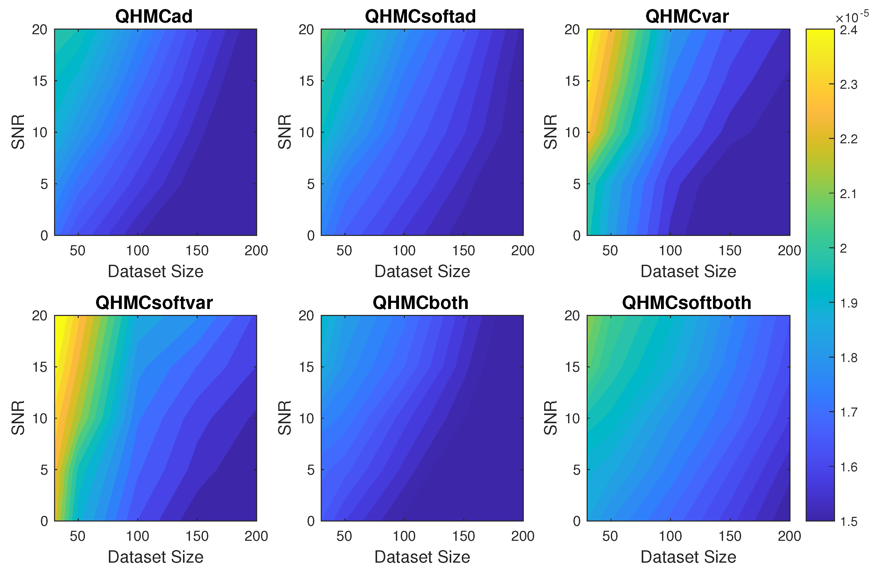
Figure 2.
Time comparison of the algorithms with different SNR and data sizes for 2D Poisson example.
Figure 2.
Time comparison of the algorithms with different SNR and data sizes for 2D Poisson example.
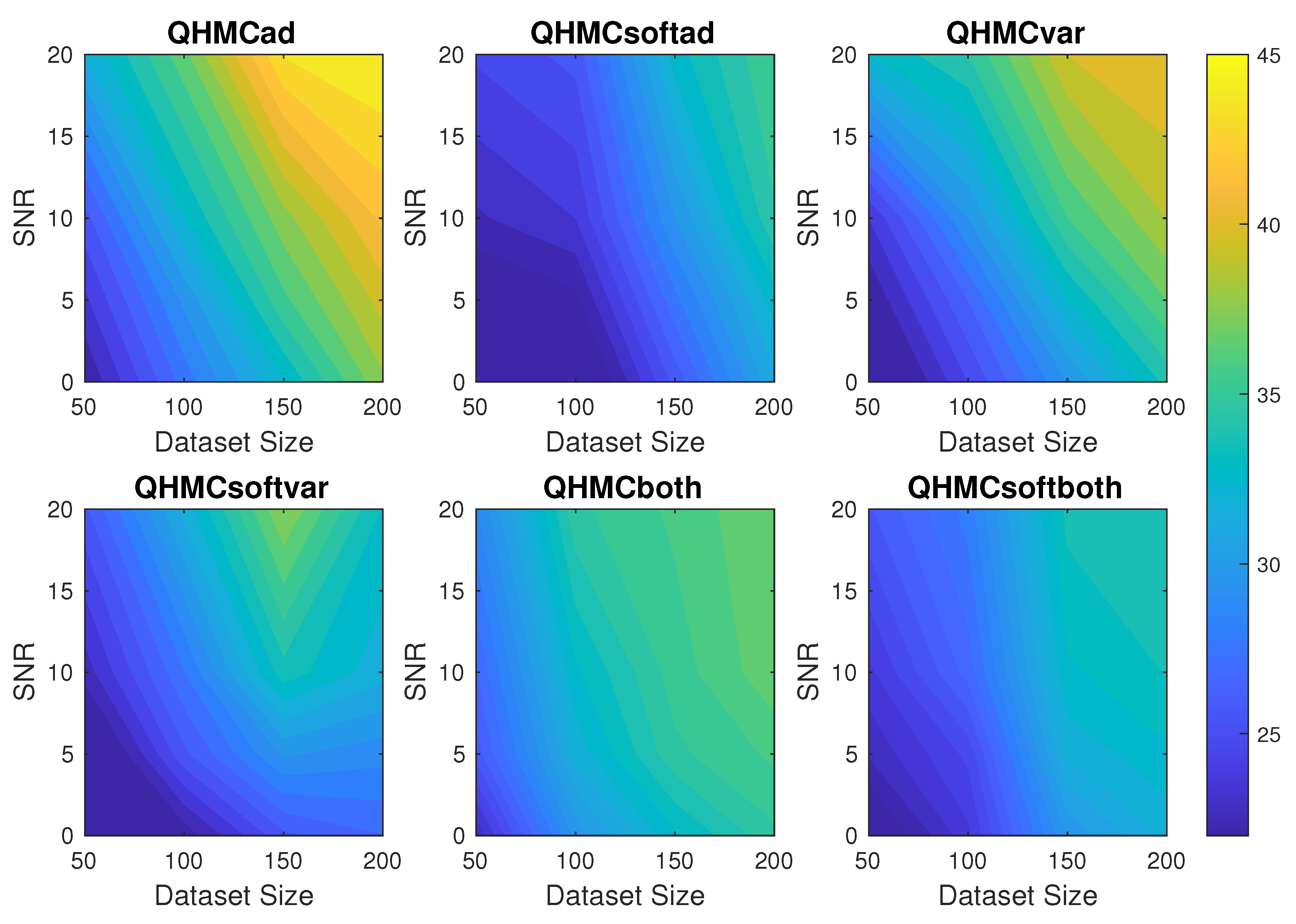
Figure 3.
Relative error of the algorithms with different SNR and data sizes for 10D Poisson example.
Figure 3.
Relative error of the algorithms with different SNR and data sizes for 10D Poisson example.
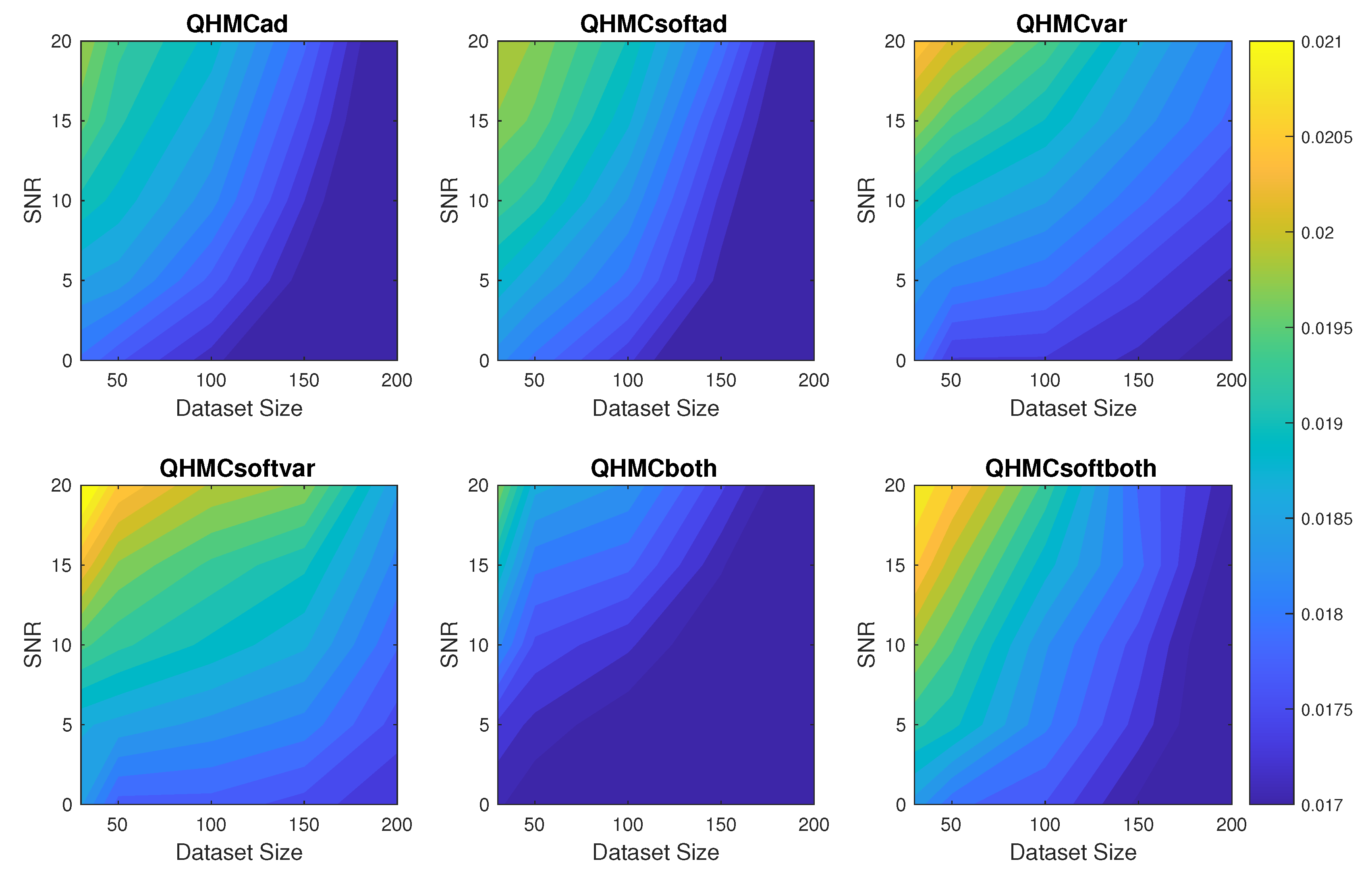
Figure 4.
Time comparison of the algorithms with different SNR and data sizes for 10D Poisson example.
Figure 4.
Time comparison of the algorithms with different SNR and data sizes for 10D Poisson example.
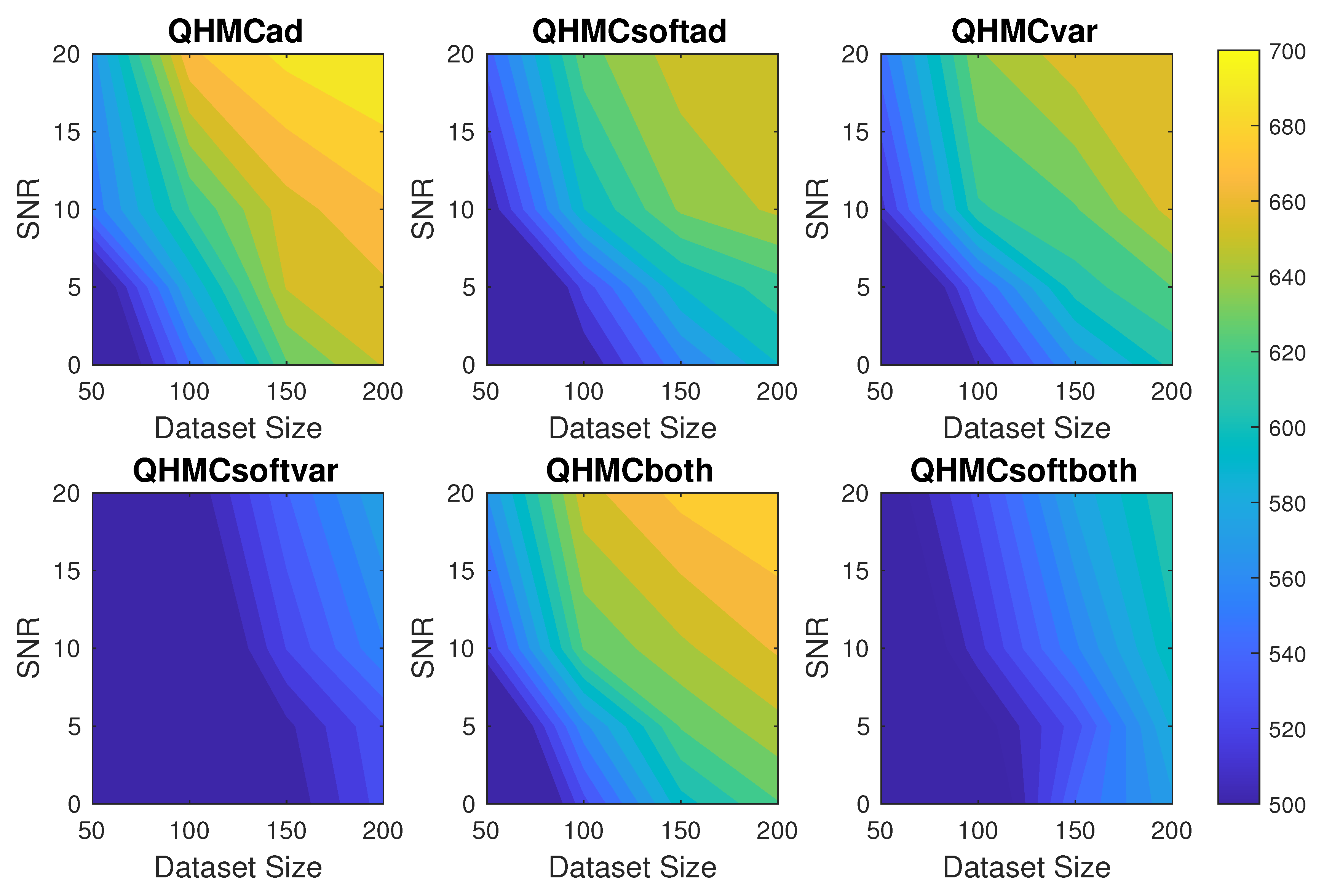
Figure 5.
The change in relative error while adding constraints, heat equation.
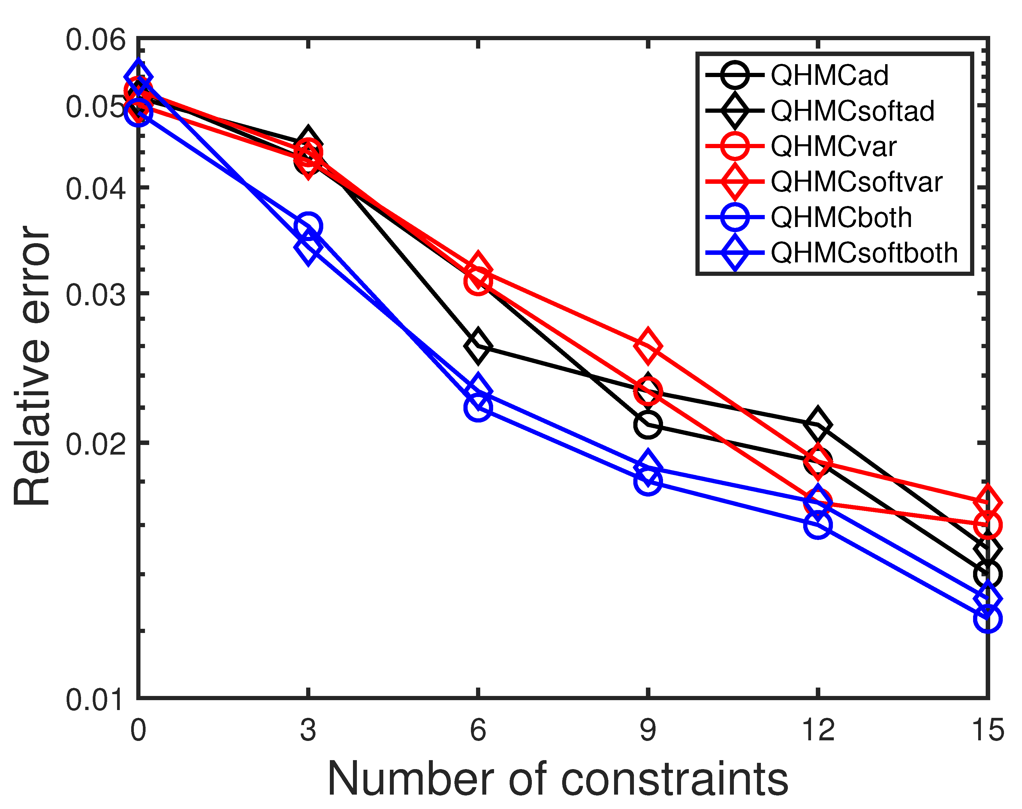

Table 1.
Comparison of methods, 2D Poisson.
| Method | Error () | Time(s) | Method | Error | Time(s) |
|---|---|---|---|---|---|
| QHMCad | 0.15 | 13.2 | HMCad | 0.19 | 16.0 |
| QHMCsoftad | 0.17 | 10.1 | HMCsoftad | 0.21 | 15.4 |
| QHMCvar | 0.16 | 11.5 | HMCvar | 0.21 | 16.4 |
| QHMCsoftvar | 0.19 | 9.2 | HMCsoftvar | 0.22 | 13.1 |
| QHMCboth | 0.14 | 12.4 | HMCboth | 0.17 | 14.3 |
| QHMCsoftboth | 0.15 | 9.5 | HMCsoftboth | 0.19 | 11.3 |
Table 2.
Comparison of methods, 10D Poisson.
| Method | Error | Time(s) | Method | Error | Time(s) |
|---|---|---|---|---|---|
| QHMCad | 0.022 | 745.2 | HMCad | 0.027 | 790.3 |
| QHMCsoftad | 0.025 | 701.7 | HMCsoftad | 0.030 | 755.1 |
| QHMCvar | 0.023 | 728.5 | HMCvar | 0.032 | 751.4 |
| QHMCsoftvar | 0.026 | 698.2 | HMCsoftvar | 0.034 | 733.3 |
| QHMCboth | 0.017 | 726.3 | HMCboth | 0.025 | 762.2 |
| QHMCsoftboth | 0.020 | 718.2 | HMCsoftboth | 0.029 | 803.3 |
Table 3.
Comparison of methods, 3D heat equation.
| Method | Error | Time | Method | Error | Time |
|---|---|---|---|---|---|
| QHMCad | 0.031 | 39s | HMCad | 0.036 | 52s |
| QHMCsoftad | 0.042 | 30s | HMCsoftad | 0.051 | 41s |
| QHMCvar | 0.032 | 32s | HMCvar | 0.045 | 44s |
| QHMCsoftvar | 0.042 | 26s | HMCsoftvar | 0.051 | 35s |
| QHMCboth | 0.027 | 43s | HMCboth | 0.036 | 56s |
| QHMCsoftboth | 0.031 | 28s | HMCsoftboth | 0.049 | 39s |
Disclaimer/Publisher’s Note: The statements, opinions and data contained in all publications are solely those of the individual author(s) and contributor(s) and not of MDPI and/or the editor(s). MDPI and/or the editor(s) disclaim responsibility for any injury to people or property resulting from any ideas, methods, instructions or products referred to in the content. |
© 2025 by the authors. Licensee MDPI, Basel, Switzerland. This article is an open access article distributed under the terms and conditions of the Creative Commons Attribution (CC BY) license (http://creativecommons.org/licenses/by/4.0/).
Copyright: This open access article is published under a Creative Commons CC BY 4.0 license, which permit the free download, distribution, and reuse, provided that the author and preprint are cited in any reuse.


