Submitted:
02 January 2025
Posted:
07 January 2025
You are already at the latest version
Abstract
The distinction between descriptive statistics and statistical modelling via probability theory is not always as useful as presented in textbooks. In this paper we take confidence intervals as an example. These intervals are defined for statistical models and are used for hypothesis testing. We propose to define slightly different intervals based on ideas based on cross-validation and on the bootstrap method. These intervals will be defined in a purely descriptive manner and that has an interpretation directly related to the sample at hand. Although these new resampling intervals have descriptive definitions they can be used for testing in just the same manner as confidence intervals. The new intervals are of particular relevance in cases where the sample cannot be modeled by an infinite sequence of iid variables. In order to compare cover probabilities we suggest to randomize the sample size. We demonstrate that both the new resampling intervals as well as z-intervals, Wilson intervals, and likelihood ratio intervals get better coverage probabilities if we use additive smoothing.
Keywords:
Additive smoothing
; bootstrap
; confidence interval
; cover probability
; cross-validation
; descriptive statistics
; likelihood ratio interval
; resampling
; Wilson interval
MSC: 62A01; 62F40
1. The Established Approach
Teaching in elementary statistics is often structured as follows. One starts with descriptive statistics, and part of this teaching will begin in elementary school. Various representations of data are studied with tables and diagrams as the most important types of representation. Then the notion of a descriptive statistic is introduced. It is easy to explain that the sample average, median, and other quantiles have important applications. It is much harder to explain why the variance and standard deviation formulas have exactly the form they have. In particular, it can be difficult to argue in favor of the Bessel correction. Hopefully, the teacher is aware that a correct explanation would involve the theory of Gaussian models and that the use for data that is not Gaussian is justified by the Central Limit Theorem. We see that methods in ’descriptive’ statistics may be motivated by ideas not considered part of descriptive statistics.
The subsequent topic use to be probability theory. The primary examples use to involve dice and card games, where the uniform distribution can be used. At high school level one can introduce a more abstract notion of probability. Frequentist interpretations, Bayesian interpretations, and other interpretations may be discussed. Elementary distributions like the binomial distributions and the hypergeometric distributions are introduced. The law of large numbers in one of its simple formulations can be proved at this level. Continuous distributions can be introduced in a precise manner for students who are well-versed in elementary calculus. The Gaussian distributions can be defined, but their properties are beyond the high school level. Even a precise formulation of the Central Limit Theorem for iid sequences is at the university level, and so is a proof of this important theorem.
Simple statistical tests are part of the curriculum of high school mathematics in many countries. Here we will focus on the part of test theory related to confidence intervals, so we will examine the definition of confidence intervals in a simple setup.
Definition 1.
Let denote a sequence of iid random variables distributed according to the measure where denotes some real parameter in the open interval Let denote a significance level. Then the notion of a confidence interval is defined as a function that maps samples into sub-intervals of Θ in such a way that
for all values of .
For the Gaussian location family with unknown and known this definition works fine with confidence intervals for given by
The Gaussian density is symmetric around so it is natural to require that the confidence intervals are symmetric around If we drop the requirement that the confidence interval is symmetric, then there are many ways of defining confidence intervals for the Gaussian location family so even in this simple case, confidence intervals are not uniquely determined by the definition.
The next example to consider is estimation of the unknown success probability p for a binomial distribution. Usually the observed relative frequency is used as estimator for p because it is the maximum likelihood estimator. In this case one cannot define confidence intervals according to the above definition, and this is the case for all exponential families of discrete distributions. One may try to repair this problem by replacing = by ≈ in Definition 1 or by replacing = by an inequality or both upper and lower bounds. If one makes such a change to Definition 1, the problem with lack of uniqueness in the definition of confidence intervals become much more prominent. Thus, there are many competing ways to calculate confidence intervals for the success probabilities of binomial distributions. Often textbooks introduce the z-intervals given by
as the basic method. There are many alternative methods: Clopper-Pearson intervals, Wilson score intervals, Agresti-Coull intervals etc. In addition, there is the Jeffreys interval that also works well, but it is formally a credence interval as defined in Bayesian statistics, so it requires a prior distribution on the success probability and on an elementary level the choice of prior may be difficult to justify.
Without a clear definition of a confidence interval it becomes impossible to judge whether a specific interval is a 95 % confidence interval for a specific dataset. For programming interactive statistics exercises about confidence intervals this problem becomes very prominent. Which formulas should be considered as valid for which sample sizes and what should be the acceptable tolerance? The only solution that will work in the classroom is to require that the students use a specific formula and say that only answers produced by this formula will be considered as valid, although other formulas may provide better results regarding cover probabilities.
In conclusion, the usual definition works well for Gaussian distributions, but it fails already for the binomial distributions. For more complicated models the situation becomes so complicated that it is never handled at an elementary level.
On an advanced level at a statistics course at university the students may learn how to handle some of these problems by bootstrap methods. The idea is to use computers to make simulations in cases where no formulas for confidence intervals are available. One replaces the unknown distribution by the empirical distribution of the sample and then sample from that distribution. Similar ideas are used in cross validation.
We will apply three separate ideas to overcome the above mentioned problems. The first idea is to randomize the sample size in order to avoid fluctuations in the cover probabilities. This will make it easier to compare the performance of different confidence intervals and it has direct consequences for how sampling should take place. The second idea is to replace the maximum likelihood estimator of p by the Krichevski-Trofimov estimator of a similar smoothening of data. Then we introduce resampling intervals as a part of descriptive statistics. These intervals have an interpretation without any reference to iid sequences. Finally we combine the idea of resampling intervals with random sample sizes and smoothing, and we illustrate that these resampling interval have good performance as confidence intervals.
2. Randomizing the Sample Size
We consider a situation where we assume that where n is known but p is unknown. A z-interval with confidence level can be calculated by formula (1). Following the standard definition of a 95 % confidence interval for each we should calculate the cover probability
where and compare the cover probability with the confidence level. According to the usual definition, a repetition of an experiment with sample size n the repetitions all have sample size n.
If the distribution of X is approximated by a Gaussian distribution then the point probability of each of the endpoints of the confidence interval can be approximated by
This will give fluctuations in the cover probability of this order. As a rule of thumb we should only use z-intervals if so that the fluctuations are less than
We should note that the problem with the fluctuations do not disappear if we use Wilson intervals, Clopper-Pearson intervals, or some other of the many formulas used to calculate confidence intervals. The fluctuations make it difficult to compare the different formulas for confidence intervals.
Figure 1.
The fluctuating cover probability (black) for the z-interval for as function of the sample size n. The confidence level is 95 %. The red curve is a plot of mean cover probability if the sample size N is a random variable with the probability distribution
Figure 1.
The fluctuating cover probability (black) for the z-interval for as function of the sample size n. The confidence level is 95 %. The red curve is a plot of mean cover probability if the sample size N is a random variable with the probability distribution
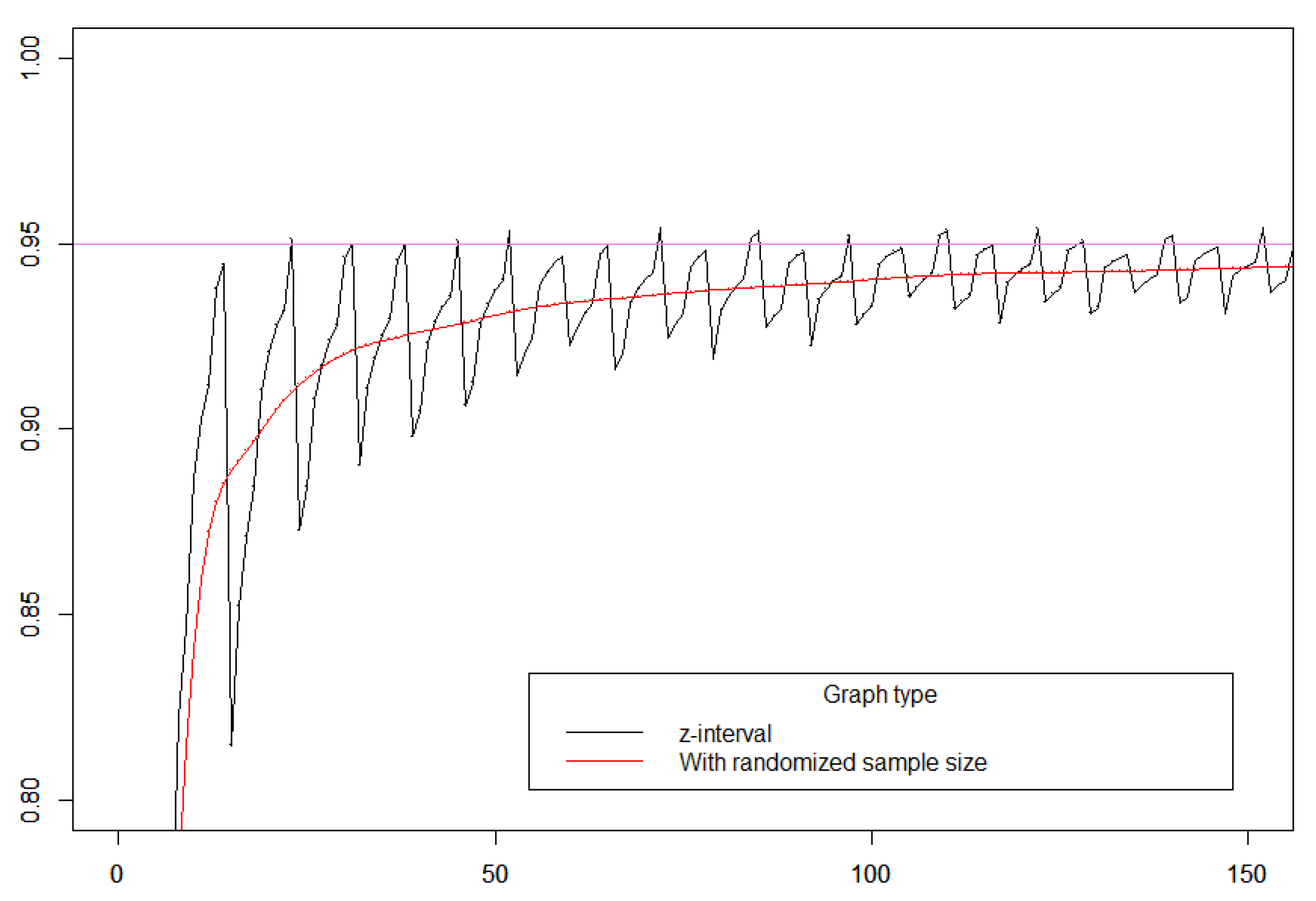
We will change the notion of a repetition of an experiment in order to handle the problem with the fluctuating cover probabilities. Instead of keeping n fixed with the same value as in the observed sample, we replace n by a randomized sample size N approximately equal to Our preferred method for randomization is to replace n with a Poisson random variable N with mean n, i.e.
In principle one could randomize the sample size according to other distributions than Poisson distributions, but the Poisson distributions should be our default choice for two reasons. The first reason is that in many cases the Poisson distributions are good models for how random sample sizes may come about in the real world. The second reason is that if X is a mixture of binomial distributions where and p is fixed then Another way to express this is that the p-thinning of is so that the family of Poisson distributions is closed under thinning. In [1] it is argued that the idea of using randomized sample sizes should play a prominent role in the foundation of probability theory. Further arguments are given in favor of using a Poisson distribution as distribution of the sample size can be found in that paper.
The idea of randomizing the sample size should not only be seen as theoretical tool to smooth out some oscillations. The idea can be implemented in statistical practice. For instance, instead of sampling until a prespecified number of samples has been achieved, one may sample for a certain amount of time. In practice this is already what often happens.
The idea of smoothing out fluctuations was also used in ([2], Section 3.2 and Figure 6), but in that paper the authors took a uniform mean of success probabilities This idea is problematic for a frequentist interpretation of probability, where the success probability p has a specific but unknown value. The idea is also problematic from a Bayesian point of view, where one may prefer Jeffreys’ prior over rather than the uniform distribution. In any case, it is difficult to see how a specific distribution of the success probability p would correspond to any particular sampling practice.
There are various methods for computing confidence intervals, and if we fix n in our definition of cover probability, the different methods are difficult to compare due to fluctuations. As we will illustrate, the situation becomes much more clear, if we randomize the sample size. For each method the performance is bad for very small sample sizes.
2.1. Wilson Interval vs. z-Interval
If we want to make a Goodness-of-Fit test of the null-hypothesis and we observe x success in a sample of size n then we can use the -statistic
We accept if the observed value of the -statistic is below the critical value . The Wilson interval is obtained by solving the inequality
with respect to The formula becomes somewhat complicated, but with modern software this is no problem. The z-interval is obtained by solving
where . This gives a simpler formula, but it corresponds to using rather than as a statistic for a Goodness-of-Fit test.
As we see in Figure 2 the Wilson interval is far superior to the z-interval. This was also the conclusion in [2] so we will not go further into this, but we should note that the comparison is much more clear when we randomize the sample size. If the sample size below 20 then the Wilson interval does not perform well. There are several ways to handle this problem, but we will not go into a discussion here, since we will make further modifications of our definitions in subsequent sections.
2.2. Likelihood Ratio Intervals
The likelihood ratio intervals are obtained by inverting the likelihood ratio test that is also called a -test. The -test is given by the statistic where the information divergence (KL-divergence) is given by
For most relevant values of and the Wilson interval and the likelihood ratio interval perform equally well [2]. This is illustrated in Figure 2.
For high confidence levels and large sample sizes the likelihood ratio intervals systematically perform better than the Wilson intervals. To understand why the likelihood ratio interval performs better for high significance levels, we introduce the signed log-likelihood by
This inequality implies that the distribution of the statistic is close to a -distribution even far large deviations. The same property does not hold for the -statistic [5]. High confidence levels are for instance used in high-precision physics, where the standard is sometimes used [6]. The standard corresponds to a significance level of about . The good performance of the likelihood ratio interval for high confidence levels is illustrated in Figure 3.
3. Choice of Estimator
3.1. Additive Smothing
The z-interval for the success probability p is based on the the maximum likelihood estimate . For an iid sequence of observations we may predict the next bit based on the previous bits. If we use the maximum likelihood estimate of the observed bits as a predictor for the next bit, we will overfit. To overcome this problem, Laplace suggested using
as estimator for the probability of the next bit being a success given that the number of successes that have been observed is x and the number of observed bits is n. The estimator (2) is called the Laplace estimator and the use is called Laplace law of succession [7]. The Laplace estimator is a special case of additive smoothing given by
The use of additive smoothing is equivalent to using the -distribution as prior on where denote the parameters of the -distribution. If the prior distribution is and x success have been observed in n observations, then the posterior distribution is The mean value of the distribution is and from a Bayesian point of view this should be the posterior estimate of
One may now ask if any specific value of is better than other values in some sense. Krichevski and Trofimov have proved that is optimal from an information theoretic point of view [8]. The estimator
is the so-called Krichevski-Trofimov estimator with . It minimizes both the asymptotic minimax redundancy and the minimax regret ([9], Chapter 9). The Krichevski-Trofimov estimator corresponds to using as prior distribution, which is also Jeffreys’ prior on the family of binomial distributions [10,11,12].
3.2. Smoothed z-Interval
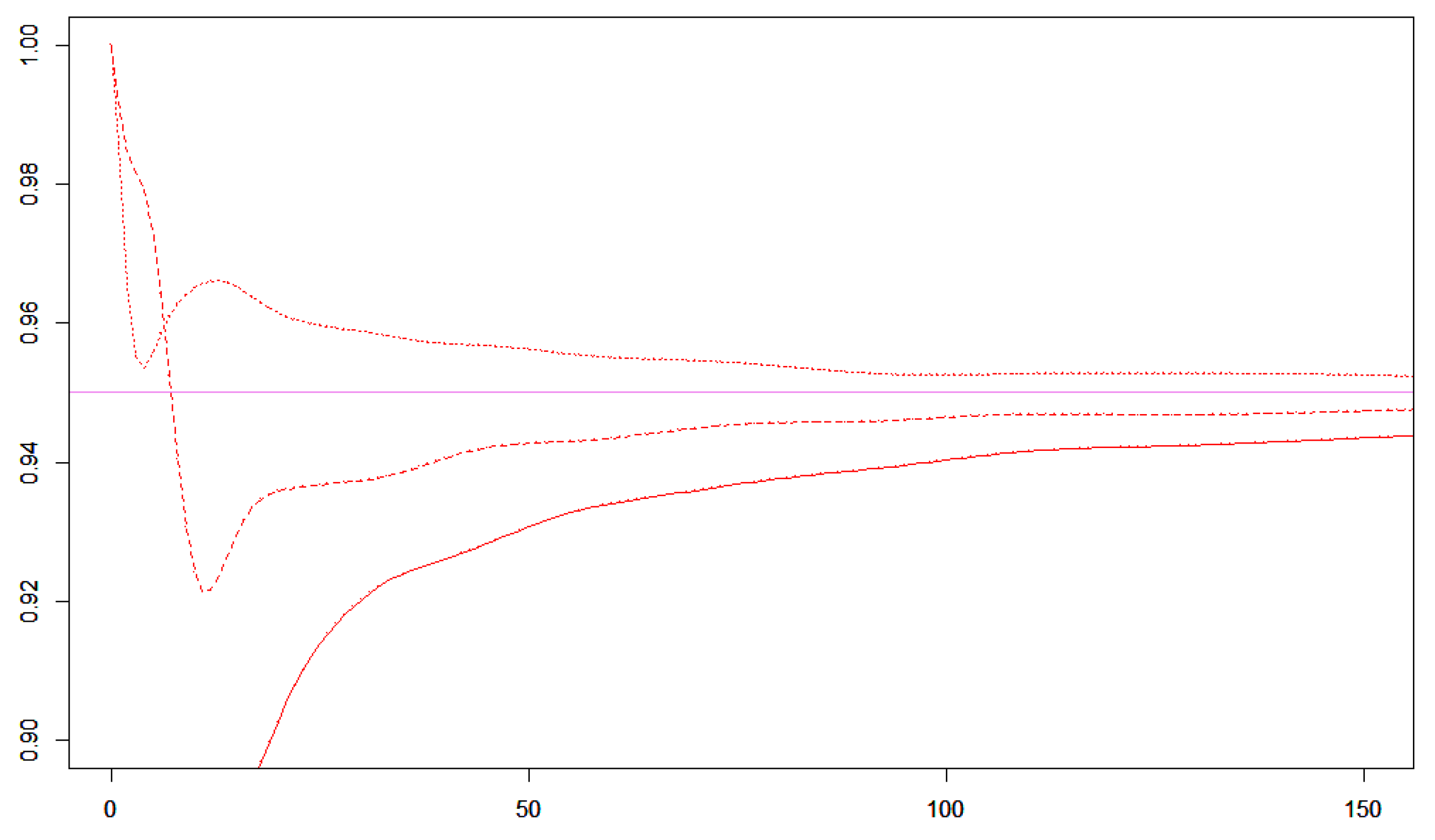
If we replace x with and replace n with in the formula for the z-interval, then we get a smoothed z-interval. The smoothed z-intervals have a significantly better cover probability than the z-intervals without smoothing as illustrated in Figure 4.
The Wilson intervals performs well, but the formula is complicated. The Wilson intervals are centered around For this reason, Agresti and Coull have suggested using additive smoothing with [13]. The Agresti-Coull interval is calculated by replacing x by and replacing n by in the formula for the z-interval. As we see in Figure 4 smoothing with the Krichevski-Trofimov estimator seems to overfit but the Agresti-Coell interval seems to underfit. Some fine-tuning of the smoothing may give values of the cover probability that are even closer to the nominal value, but we will not go into this in the present paper.
3.3. Smoothed Wilson Intervals
Wilson intervals can also be smoothed by replacing x with and replece n with in the formula for the Wilson-interval.
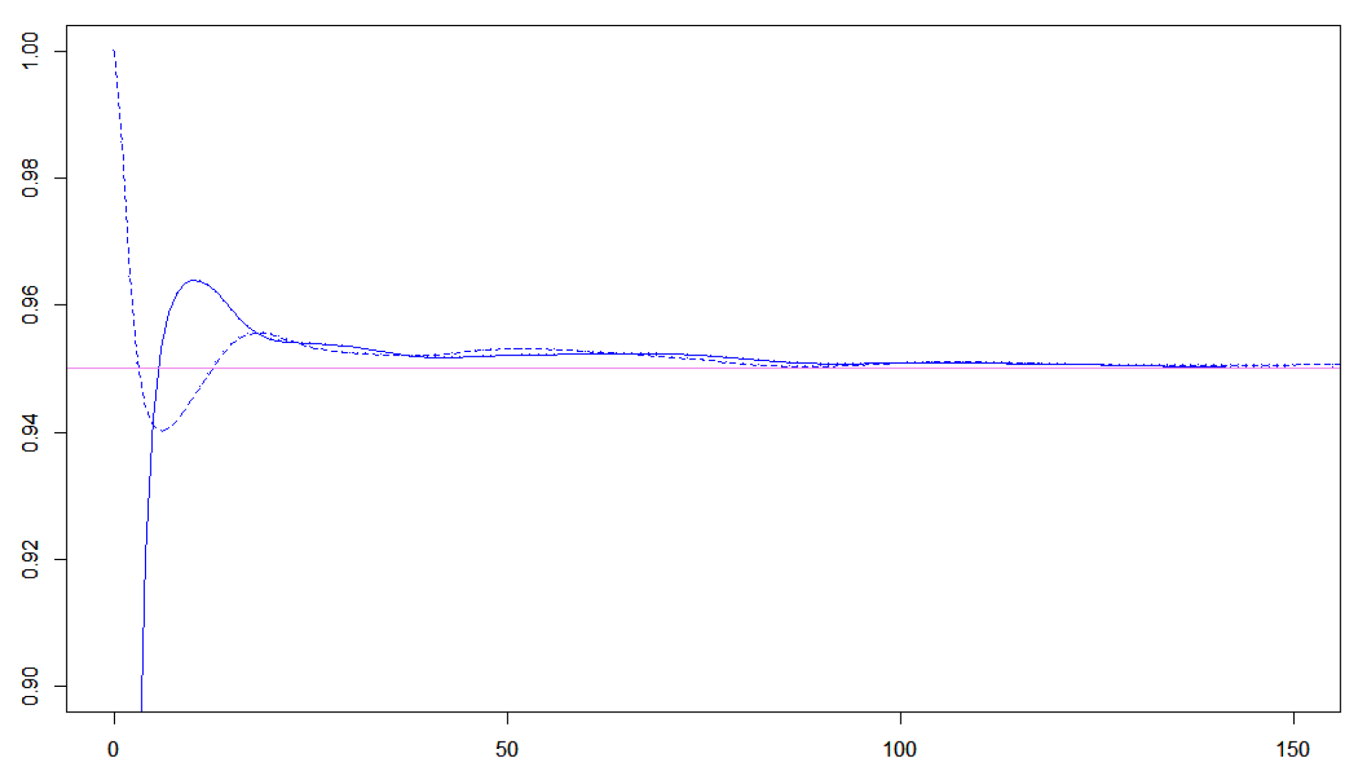
Figure 5.
In this plot and The blue curve is the Wilson interval and the dashed blue curve is the same interval with the Krichievski-Trofimov correction.
Figure 5.
In this plot and The blue curve is the Wilson interval and the dashed blue curve is the same interval with the Krichievski-Trofimov correction.
3.4. Smothed Likelihood Ratio Intervals
We suggest that we use
for testing Goodness of Fit where is the Krichevski-Trofimov estimator. We get confidence intervals by solving the equation with respect to p where the divergence is equal to the critical value . As illustrated in Figure 6 the cover probability will be above the nominal value while the likelihood ratio interval will be below the nominal value.
Figure 6.
In this plot and The cyan curve is cover probability for the likelihood ratio interval and the blue curve is the same interval with the Krichievski-Trofimov correction.
Figure 6.
In this plot and The cyan curve is cover probability for the likelihood ratio interval and the blue curve is the same interval with the Krichievski-Trofimov correction.

4. Resample Intervals
4.1. Split Sample Intervals
In the definition of a confidence interval, the idea is to compare a descriptive statistic based a sample with a similar descriptive statistic of the whole population. One may for instance compare the average height of a sample of 100 Danes with the average height of all 5.8 mio. Danes. We assume that the probability distribution is exchangeable and that the statistic of interest is invariant under permutations. As a rule of thumb, one does not have to distinguish between sampling with and without replacement as long as the sample is less than 5 % of the whole population. In order to make the mathematical theory run smoothly, one often assumes that the population is infinite, i.e. we sample from a sequence of iid random variables.
The assumption of having an infinite iid sequence is of cause problematic in practice, but in cases with systematic scientific experiments it may be justified. The notion of an infinite sequence should just be understood as an abstract way of saying a sequence that can be extended with no upper bound on the length [14]. In applications in social sciences and humanities, the notion of a dataset being a sample from a much larger population is often problematic. It is in particular problematic if we require that the population should be at least 20 times as large as the sample. For instance, we may make statistics about the size of the stones at Stonehenge, but Stonehenge is not a sample of a large population of Stonehenges. Maybe we will be lucky to find the remains of one or more Stonehenge like structures, but finding 20 or more Stonehenges is completely unrealistic. There have actually been found a number of Stonehenge like structures but they are quite different on many parameters, so we can only find many Stonehenge like structures if drop the idea of exchangeability.
Another problem often experienced when using statistical methods in social sciences and humanities is that some of the data points in the dataset are problematic. Some may argue that a specific data points should be removed from the dataset. If it is just one or a few data point that are somewhat problematic one can simply removed these datapoint, but the situation is often more complicated. Sometimes one has a large dataset that contains some pattern that are only visible by statistical means. For each data point there are some issues that may be used as argument that exactly this datapoint should be excluded. The datapoint may be the result of a study that is quite old, the data point may be the result of an investigation that was not done with the amount of care that one desire, the data point may rely on some interpretation that have been disputed, etc. If all datapoints are removed the pattern disappears, so we may want to handle this problem in a different manner than removing specific points.
Usually we compare the statistic of a sample with a similar statistic for a much larger sample, but here we will compare the statistic for the sample with a similar statistic for a subsample. This idea is closely related to the idea of cross validation. For simplicity we will assume that the sample size is even and that we are interested in the sample average.
Definition 2.
Let denote a sample. Let Then a split sample intervalfor a descriptive statistic is defined as interval from the -quantile to the -quantile of the dataset consisting of descriptive statistic calculated for of all subsamples of of size
The idea is that we look at how sensitive the descriptive statistic is to taking a subsample of half the size of the original sample. If a datapoint is problematic then this datapoint will only appear in half of the subsamples. Therefore the width of the split sample interval will reflect whether problematic data points are included or excluded.
Assume that a sample of size contains ℓ invalid data points and valid data points with average . As an example we may consider the important situation where If then the probability that a certain spilt sample contains no invalid data points is at most . Of these split samples without invalid data points half will have an average less than and half will have average greater than Therefore the probability that that a split sample has an average less is at least Similarly the probability that a split sample has an average greater than is greater than 0.025. Hence the probability that the 95 % split sample interval contains is greater than One may say that a 95 % split sample interval contains the average of the valid data points with probability greater than 95 % as long as the data set contains at most 4 invalid data points. This holds even if the invalid data point have very extreme values. In practice very extreme values should be examined carefully to check if something is wrong. If something is wrong the problematic data points should be declared an outliers and removed from the dataset. If we have a systematic way of identifying extreme values as outliers and exclude then, then the probability that belongs to the split sample interval is greater than 95 % even if the number invalid data points in a data set could be much greater than 4. Each criteria for declaring outliers require its own analysis, which we will not go into in this paper.
If the sample size is then the number of split samples is given by the central binomial numbers These numbers grow like
Students should be able to do the split sample statistics by hand as long as is less than 6 or 8. For sample sizes up to 24 a computer should be able to run through all the different combinations. For larger datasets a computer may do the calculations by some Monte Carlo simulations. We should note that here the simulations play a very different role than simulations use to play. We are not simulating an abstract experiment with iid outcomes. We are using the simulation as a method for doing approximate calculations. In this sense, our use of simulations is part of numerical analysis rather than an attempt to simulate an abstract truth.
In special cases the calculation of split sample intervals can be done exactly for large sample sizes.
Example 1.
Let be a sample of a binary variable, i.e. Then
where k is the number of ones in the sample. The average of a subsample of size n is a random variable Y such that has a hypergeometric dsitribution with parameters and the split sample interval is given by the quantiles of the this hypergeometric distribution. Thus the split sample interval for binary variables can be calculated by elementary means without any knowledge of Gaussian distributions.
Theorem 1.
Let denote a sample of size with mean and variance Let L be the random variable that denotes the sum of elements in a subsample of size Then the distribution of is symmetric around and in particular the skewness of is zero. The variance of is
Proof.
Our first observation is that the sample average lies in the split sample interval. Actually, the split sample interval is always symmetric around the sample average. The reason is that the average of a subsample of size n and the average of the complementary subsample have the average of the full sample as midpoint.
Let denote a subsample of size Then Therefore
Hence
□
4.2. Bootstrap Intervals
If the sample space is small compared with the sample size then some observations will appear several times in the sample, i.e. the multiplicity is greater than one. For the split sample intervals we considered the case where some observations in the sample were problematic. If we know that an observation is invalid it should count with multiplicity zero instead of one. Here we also consider the more general situation where we both consider problematic observations that were included although they may have been excluded, and some problematic observations that were excluded but should have been included. By default each datapoint has multiplicity 1, but we want to check how sensitive our analysis is to changes in the multiplicity of the individual data points. An example from archaeology where some data point may be invalid and other data points may count with higher weight was presented in [15]. If the sample size is n then we make bootstrap samples from the sample by taking n points from the sample with replacement. Some points will not be chosen and some will be chosen with multiplicity greater than 1.
Definition 3.
Let denote a sample and let denote some exchangeable statistic. Let Then a exact bootstrap intervalis defined as interval from the -quantile to the -quantile of the dataset consisting of f on all bootstrap samples from .
Compared with the split sample interval the bootstrap interval can be defined for any exchangeable statistic because the sample size of the bootstrap sample is the same as the original sample size. In addition, the definition works equally well for even and odd sample sizes.
Example 2.
If the variable is binary with values 0 and 1, and the size of the dataset is n then the distribution of bootstrap sample is where x denotes the number of 1’s in the dataset. The end points of the bootstrap interval is given by the quantiles of the binomial distribution.
If the size of the sample space has a size that is much greater than the sample size then it is highly unlikely that any observation has multiplicity greater than one. This happens for instance when the sample space is continuous. In an exchangeable setup all observations should have the same weight, but often this is not fully justified. In practice it is quite common that some observations are expected to be more representative than other observations. In principle this might be taken care of by assigning individual weights to the observations, and such individual weights may in principle assume a continuous range of values. In practice, it may be difficult to assign such weights. Instead, one may check how sensitive the conclusions are to random variations in the weights. Using a bootstrap interval one assigns weights that are Poisson distributed with mean 1 with the extra condition that the sum of the weights should add up to 1. In principle, one may consider distributions than the Poisson distribution, but since we are mainly interested in the sensitivity to changes in the weights rather than the effect of specific changes we will stick to Poisson distributions and the definition of bootstrap intervals given above.
Theorem 2.
Let denote a sample of size n with mean and variance Let L be the random variable that denotes the sum of elements in a bootstrap subsample. Then the distribution of has mean value and the variance is
Proof.
Let denote a bootstrap sample. Then . Therefore
Similarly,
□
The distribution of the average of the bootstrap samples can be approximated by a Gaussian distribution with mean and variance
Instead of using the percentile interval defined in Definition 3 we may calculate normal bootstrap intervals where the quantiles are calculated from a normal approximation of the bootstrap distribution. We consider this as a numerical technique for efficient calculations of approximate bootstrap intervals. Other variations are studentized bootstrap intervals, where one approximates by a t-distribution and adjusted percentile intervals. All the variations are well described in the literature and well implemented in the R-program. Since we consider these variations as numerical techniques rather than descriptive statistics, they will not be discussed any further.
4.3. Resample Intervals as Confidence Intervals
The resample intervals are designed to describe how sensitive a descriptive statistic is to modifications of the data set. The question is whether resample intervals can be used as confidence intervals, i.e. if the resample interval of a sample from a population contain the descriptor of the population with high probability.
We will use a 95 % bootstrap resampling interval for a sample from a binomial distribution as example. We will use the likelihood estimate as estimator and use the interval from the 2.5 % quantile to the 97.5 % quantile of the distribution as 95 % resample interval. As usual, the cover probability will fluctuate up and down, but by randomizing the sample size we get rid of these fluctuations.
Figure 7.
Cover probability of a 95 % bootstrap interval for (black). The green curve is the average over a random sample size that is Poisson distributed with mean
Figure 7.
Cover probability of a 95 % bootstrap interval for (black). The green curve is the average over a random sample size that is Poisson distributed with mean
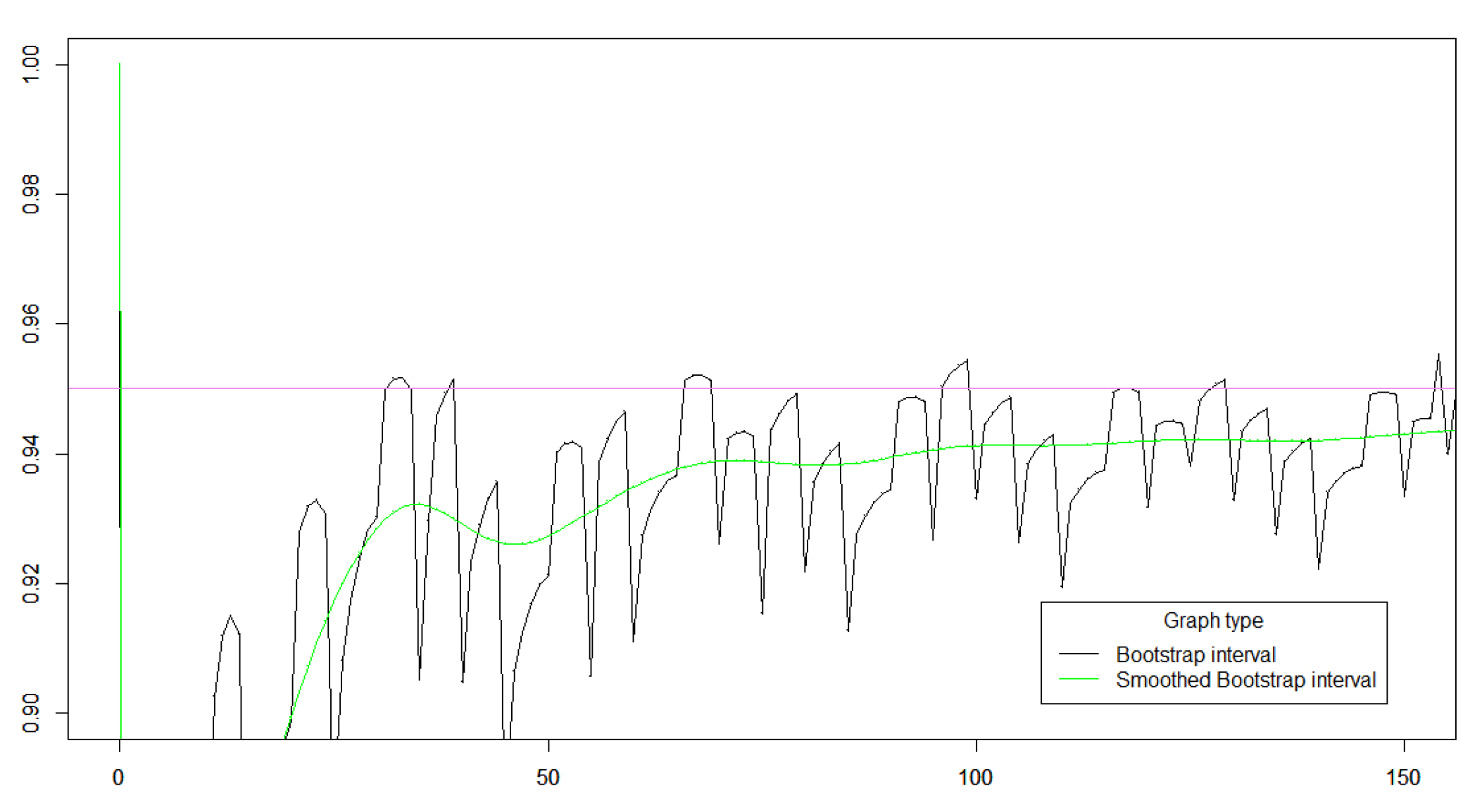
The average cover probability is very similar to the cover probability of the smoothed z-interval. Therefore the bootstrap intervals with Agresti-Coell smooting can be recommended as confidence intervvals whenever the Agresti-Coell interval can be recommended. The advantage of the bootstrap intervals is that they have an interpretation without any reference to infinite iid sequences and they can be calculated without any Gaussian approximation.
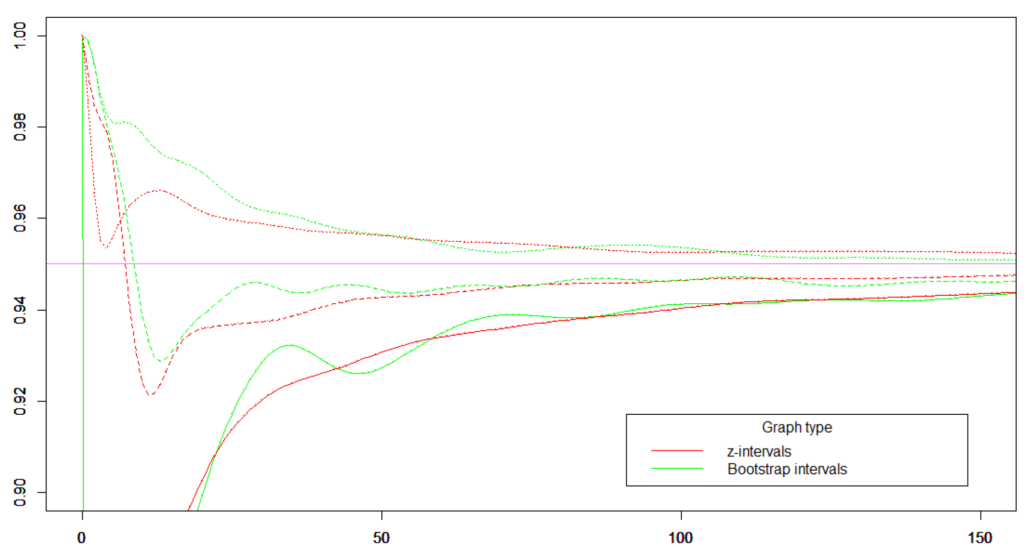
Figure 8.
Cover probability of a 95 % interval for The green curves are cover probabilities for the bootstrap interval without smoothing (solid), with Krichevski-Trofimov smoothing (dashed), and with Agresti-Coell smooting (dotted). The red curves are cover probabilities for the z-interval without smoothing (solid), with Krichevski-Trofimov smoothing (dashed), and with Agresti-Coell smooting (dotted).
5. A New Approach
With randomized samples, improved estimators, and resample intervals one can teach elementary statistics in a new way. First, descriptive statistics is introduced as usual. Then, resample intervals are introduced in order to quantify how sensitive a descriptive statistic is to modification of the dataset. The idea behind the split sample interval is very easy to describe. The idea behind bootstrap intervals is somewhat more advanced since it involves the concept of multiplicity, but it is still much easier to explain than the usual notion of a confidence interval. Whether one use slit sample intervals or bootstrap intervals on an elementary level will be a matter of taste. In practice, split sample intervals and beeotstrap intervals will be quite similar.
If a dataset is a sample from a population we may be interested in a descriptive statistic for the population. For this we introduce an estimator for the statistic. This estimator may be given by the same formula as the formula for the descriptive statistic, or one may use a modified formula. Now, a resample interval may be used as confidence interval for the statistic. The resample intervals can be used for testing without knowing cover probabilities and significance levels. Proofs that resample intervals have cover probability tending to for the sample size tending to infinity can be postponed to a more advanced level.
Sampling should by default be done with random sample size. Using random sample sizes will average out fluctuations in the cover probabilities, but there are other reasons for leaving the paradigm of fixed sample size as discussed in the literature on safe testing [16].
In the present paper we have introduced resampling intervals with in each tail. If the descriptive statistic is a vector this approach does not work. For vectors one should define a resampling region around the value of the descriptive statistic. Such a region should be defined using some distortion function like we used -divergence in the definition of z-intervals and Wilson intervals and like we used information divergence to define likelihood ratio intervals. This idea can also be used for a 1 dimensional statistic and it may actually lead to resample intervals with better cover probabilities.
Funding
This research received no external funding.
Institutional Review Board Statement
Not applicable.
Data Availability Statement
The original contributions presented in this study are included in the article. Further inquiries can be directed to the corresponding author.
Conflicts of Interest
The authors declare no conflicts of interest.
Abbreviations
The following abbreviations are used in this manuscript:
| bin | Binomial distribution |
| iid | Independent identically distributed |
| Po | Poisson distribution |
References
- Harremoës, P. Probability via Expectation Measures. Preprints 2024. [Google Scholar] [CrossRef]
- Brown, L.D.; Cai, T.T.; DasGupta, A. Interval Estimation for a Binomial Proportion. Statistical Science 2001, 16, 101–133. [Google Scholar] [CrossRef]
- Zubkov, A.M.; Serov, A.A. A Complete Proof of Universal Inequalities for the Distribution Function of the Binomial Law. Theory Probab. Appl. 2013, 57, 539–544. [Google Scholar] [CrossRef]
- Harremoës, P. Bounds on tail probabilities for negative binomial distributions. Kybernetika 2016, 52, 943–966. [Google Scholar] [CrossRef]
- Harremoës, P.; Tusnády, G. Information Divergence is more χ2-distributed than the χ2-statistic. In Proceedings of the 2012 IEEE International Symposium on Information Theory, IEEE, Cambridge, Massachusetts, USA, July 2012; pp. 538–543. [Google Scholar] [CrossRef]
- Lyons, L. Five sigma revisited. Cern Courier 2023. [Google Scholar]
- Krichevskii, R. Laplace’s Law of Succession and Universal Encoding. IEEE Trans. Inform. Theory 1998, 44, 296–303. [Google Scholar] [CrossRef]
- Krichevsky, R.; Trofimov, V. The performance of universal coding. IEEE Trans. Inform. Theory 1981, 27, 199–207. [Google Scholar] [CrossRef]
- Grünwald, P. the Minimum Description Length principle; MIT Press, 2007.
- Jeffreys, H. An invariant form for the prior probability in extimation problems. In Proceedings of the Proceedings of the Royal Statistical Society, London, 1946; Volume 186, Series A; pp. 453–461.
- Clarke, B.; Barron, A. Jeffreys’ prior is asymptotically least favorable under entropy risk. J. Statist. Plan. and Inf. 1994, 41, 37–60. [Google Scholar] [CrossRef]
- Kass, R.E.; Wasserman, L.A. The Selection of Prior Distributions by Formal Rules. Journal of the American Statistical Association 1996, 91, 1343–1370. [Google Scholar] [CrossRef]
- Agresti, A.; Coell, B.A. Approximate is better than ’exact’ for interval estimation of binomial proportions. The American Statistician 1998, 52, 119–126. [Google Scholar] [CrossRef]
- Harremoës, P. Extendable MDL. In Proceedings of the Proceedings ISIT 2013, IEEE Information Theory Society, Boston, July 2013; pp. 1516–1520. [Google Scholar] [CrossRef]
- Harremoës, P. Rate Distortion Theory for Descriptive Statistics. Entropy, 25, 456. [CrossRef]
- Grünwald, P.; de Heide, R.; Koolen, W. Safe testing. Journal of the Royal Statistical Society Series B: Statistical Methodology 2024, 86, 1091–1128. [Google Scholar] [CrossRef]
Figure 2.
The red curve is the standard z-interval for and n between 0 and 150. The confidence level is 95 %. The blue curve is the cover probability of the corresponding Wilson interval and the cyan curve is the cover probability for the likelihood ratio interval.
Figure 2.
The red curve is the standard z-interval for and n between 0 and 150. The confidence level is 95 %. The blue curve is the cover probability of the corresponding Wilson interval and the cyan curve is the cover probability for the likelihood ratio interval.
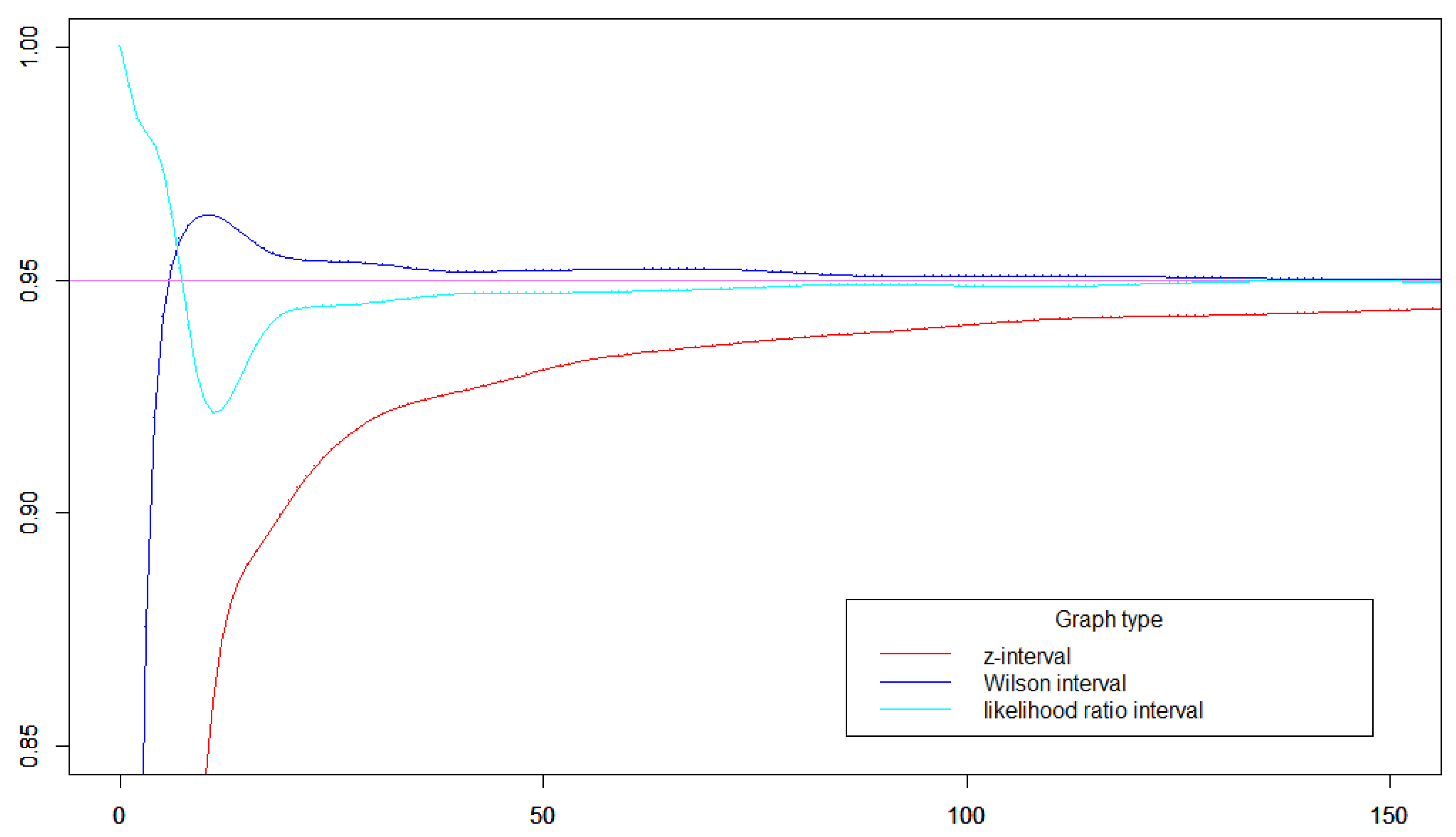
Figure 3.
In this plot the success parameter is and the confidence level is % corresponding to the standard. The blue curve is the cover probability of the Wilson interval. The red curve is the cover probability for the Agressi-Coull interval, and the cyan curve is the cover probability for the likelihood ratio interval.
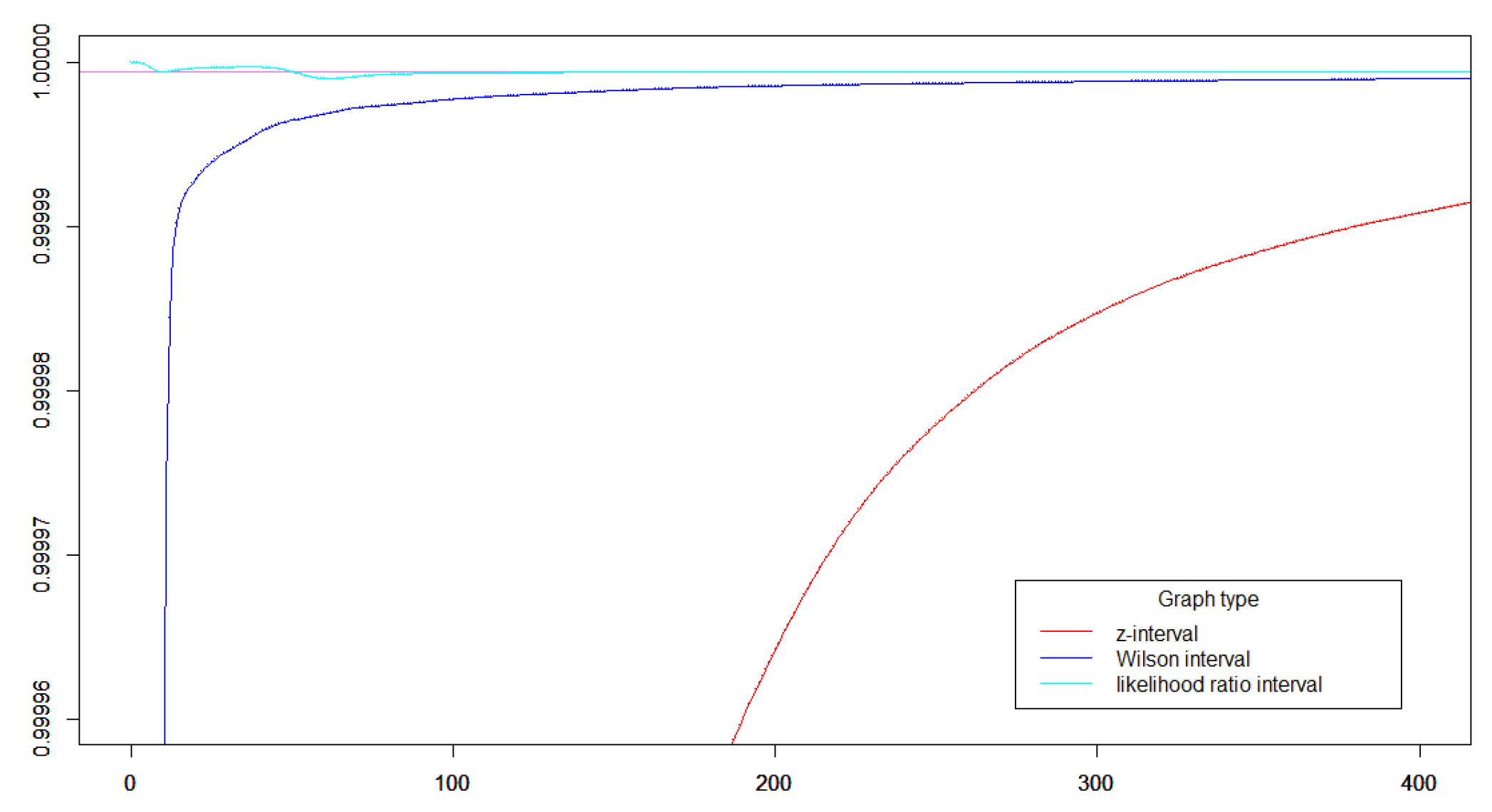
Figure 4.
In this plot and . The full red curve illustrates the cover probability of the z-intervals. The red dashed curve illustrates the z-interval smoothed with the Krichevski-Trofimov estimator. The red dotted curve illustrates the cover probability for the Agresti-Coell intervals.
Figure 4.
In this plot and . The full red curve illustrates the cover probability of the z-intervals. The red dashed curve illustrates the z-interval smoothed with the Krichevski-Trofimov estimator. The red dotted curve illustrates the cover probability for the Agresti-Coell intervals.
Disclaimer/Publisher’s Note: The statements, opinions and data contained in all publications are solely those of the individual author(s) and contributor(s) and not of MDPI and/or the editor(s). MDPI and/or the editor(s) disclaim responsibility for any injury to people or property resulting from any ideas, methods, instructions or products referred to in the content. |
© 2025 by the authors. Licensee MDPI, Basel, Switzerland. This article is an open access article distributed under the terms and conditions of the Creative Commons Attribution (CC BY) license (http://creativecommons.org/licenses/by/4.0/).
Copyright: This open access article is published under a Creative Commons CC BY 4.0 license, which permit the free download, distribution, and reuse, provided that the author and preprint are cited in any reuse.


