Submitted:
02 January 2025
Posted:
06 January 2025
You are already at the latest version
Abstract
Aiming at global path planning of mobile robot in unknown environment and how to avoid random dynamic and static obstacles in unknown environment, A path planning algorithm combining improved A* algorithm and optimized dynamic window method is proposed. The A* algorithm has a more comprehensive global path planning ability, and has a good computational speed, but also is currently the most widely used algorithm for global path planning. But the traditional A* algorithm also has many drawbacks, low search efficiency in complex environments, the existence of a large number of redundant nodes, the path is not smooth and other problems. Therefore, this paper proposes an improved A* algorithm first, which reduces the search direction, removes redundant turning points and covariance nodes, and obtains a smooth optimal planning path after Bessel curve optimization; secondly, it is optimized for the single motion state of the dynamic window method, and the safety distance is set to cope with obstacles that have a similar motion state to the robot, and the improved A* algorithm is integrated with the optimized dynamic window method, so as to meet the global planning The improved A* algorithm is integrated with the optimized dynamic window method, so as to realize obstacle avoidance in the face of random obstacles at the local position while satisfying the optimal curve in the global planning path. After simulation experiments with the traditional A* algorithm in several groups of different environments, the experimental results are obtained, the improved A* algorithm has obvious advantages in global path planning, the computation time is reduced by 40%, the search nodes are reduced by 50%, and the cost of global path search is reduced by 75%, and the fusion with the optimized dynamic window method can solve the local obstacle avoidance problem very well.
Keywords:
mobile robot
; Path planning
; Dynamic obstacles
; A* algorithm
; Dynamic window approach
1. Introduction
The key to achieving intelligent mobile robots lies in path planning and random obstacle avoidance techniques, which are essential for enabling autonomous navigation[7]. Mobile robots must navigate through a variety of unpredictable obstacles while planning the most efficient path from the starting point to the destination. In real-world scenarios, they encounter both static and dynamic obstacles with varying speeds, adding complexity to the environment. Therefore, effective path planning should not only focus on selecting the best route but also incorporate the ability to avoid random obstacles.
There are a variety of traditional path planning algorithms that have achieved significant results in different environments. Commonly used global path planning algorithms include graph-based search algorithms, sampling-based algorithms and intelligent algorithms[2]. The A* algorithm is particularly noted for its comprehensive global path planning capabilities and good computational speed, making it the most widely used algorithm for global path planning at present. Utilizing sensors to gather local environmental data while mobile robots are operating allows real-time dynamic obstacle avoidance through local path planning. The Artificial Potential Field approach and the Dynamic Window Approach are two typical local path planning algorithms[3].
Traditional A* algorithms have several drawbacks, including low search efficiency in complex environments, the presence of numerous redundant nodes, and the generation of uneven paths. Xu et al. [4] advocated replacing octal neighborhoods with unobstructed rectangular limitations and exploring the map in two directions, from the beginning and target points, respectively. Lai et al.[5] used second-order Bezier curves to optimize path length and curvature, increasing the robot’s safety coefficients while additionally adjusting the search neighborhood. Cheng et al.[6] incorporated Morphin’s technique for increased efficacy, developed a key node culling strategy to remove unnecessary nodes, and created a more appropriate heuristic function. The incorporation of these enhancement techniques shows considerable potential for improving the performance and practicality of path planning algorithms. However, challenges remain, such as inadequate path smoothing and insufficient search efficiency in complex road conditions. Robots can navigate complex areas with impressive efficiency when they are equipped with the dynamic window approach, which allows them to avoid obstacles at random while advancing. It finds wide applications in obstacle avoidance in unknown environments. However, the dynamic window approach has a disadvantage: due to the relies on a single motion state, it might become imprisoned in local optima. Furthermore, several modification strategies have been proposed to improve the evaluation function[7].
Liu et al.[8] optimize the trajectory evaluation function of the DWA algorithm to make the local path planned by the DWA algorithm smoother and more coherent, extract the key nodes from the global path, and guide the DWA algorithm to carry out the local path planning and dynamic obstacle avoidance, so that the local path is closer to the global path. Xu et al.[9] formulate a cost function based on real-world environmental information that can provide positive reinforcement when turning in the face of an obstacle, introduce a new evaluation function, and mitigate the problem of local optimization that may occur in complex situations. However, the challenge of single state of motion still persists. When facing obstacles with similar trajectories and speeds as its own, the robot often chooses to make a large-angle turn and change direction at the maximum speed, which increases the safety hazard of robot operation[10].
For the purpose to address the enduring problems that have not been resolved by specialists and researchers in the past, this work suggests a fusion algorithm for effective and secure path planning. The traditional A* algorithm is first enhanced to minimize the search neighborhood and optimize the heuristic function in order to lower search expenses[11]. Next, the path curve is optimized by removing co-linear nodes and redundant turning points. Additionally, a safe distance is established to mitigate the issue of single motion state in the dynamic window method. The proposed approach allows dynamic obstacle avoidance within the scope of global path planning by combining the regional obstacle avoidance strengths of the dynamic window method with the global planning capabilities of the A* algorithm[12].
2. A* Algorithm
2.1. Traditional A* Algorithm
The traditional A* algorithm is a widely used heuristic algorithm for path planning. It combines the strengths of existing algorithms such as Dijkstra and BFS, while addressing their limitations. The algorithm incorporates a heuristic function to estimate the overall cost of each path. The traditional A* algorithm calculates the cost value as follows:
In the formula, the actual cost from the start point to the current node is displayed by g(n), the forecast cost from the current node to the target point is indicated by h(n), and the expected total cost from the start point to the end point is represented by f(n).
In this study, we use the Euclidean distance to denote the actual surrogate value and the Chebyshev distance to denote the predicted surrogate value, which are computed as follows:
In the formula, (x1 , y1) represents the co-ordinates of the start point, (x2, y2) represents the co-ordinates of the current node n, and (x3 , y3) represents the co-ordinates of the target point.
2.2. Improvement of the A* Algorithm
2.2.1. Selection of Search Neighborhoods
The conventional A* algorithm conducts searches and selects from the 8-neighborhood grid range around a node. However, the constraints imposed by the target point’s direction result in unnecessary search ranges within the 8-neighborhood grid, leading to significant computational time and speed wastage. This study presents an approach to optimize the selection of search locations within the 8-neighborhood search direction, with the goal to enhance search efficiency and reducing the anticipated generation value.
As illustrated in Figure 1, the traditional A* algorithm searches in all 8 neighboring directions of each parent node. This approach can lead to unnecessary operations on nodes that do not contribute to the optimal path, thereby reducing search efficiency. To solve the problem of search inefficiency, this investigation provides an algorithm for dynamically allocating search direction based on the real-time target position. By minimizing operations on irrelevant nodes, this method aims to enhance the overall search efficiency.
The direction 2 and the angle α show how the line connecting the current and goal sites is oriented. The association between the direction of selection and the α value is summed up in Table 1.
The previously mentioned steps improvements to the search neighborhood can significantly reduce the number of node searches while increasing calculation speed, thereby enhancing path organizing computational efficiency. By reducing the scope of the search, the computational time is also significantly decreased.
2.4.2. Optimization Heuristic Function
The design of the heuristic function is essential to the A* algorithm’s functioning, since it has a direct influence on both the efficiency of the search process and the quality of the pathways produced, eventually deciding the algorithm’s overall performance[13]. Optimal search efficiency is achieved only when the predicted cost matches the actual cost. To balance search efficiency and route quality, use a dynamic adjustment mechanism for the heuristic function. This entails constantly updating the heuristic estimates using real-time data obtained throughout the search process, allowing the algorithm to adapt to various phases and conditions.
Let the coordinates of the current point be denoted as (x1,y1), the coordinates of the target point as (x2,y2), the distance between the current point and the target point as r, and the distance between the start point and the target point as R. In the initial state, the current point is far from the target point. At this stage, the search space is extensive and there are numerous search nodes. As the current point gradually approaches the target point, the predicted surrogate value changes. To prevent the algorithm from getting trapped in a locally optimal solution and failing to find the target point, it is crucial to reduce the weight of the predicted cost function at the appropriate time
In different environments, the weight of the heuristic function h(n) is influenced by the introduction of the obstacle occupancy ratio P. When there are fewer obstacles, the occupancy weight should be appropriately decreased. Let’s suppose that the number of obstacles in a localized region is represented by B, and the total number of grids is denoted by A. The total number of grids, denoted by A, can be expressed as follows.
The percentage of obstacles in the localized region created by the current node and the target node inside the current area is represented by the obstacle share P.
The improved heuristic function is:
When the robot is at the starting point, the distance weighting factor tends to be 1. As pathfinding progresses, this factor gradually decreases and approaches 2 when the robot is near the target point. According to the characteristics of the logarithmic function, the logarithmic attenuation factor is initially quite large but gradually decreases as pathfinding proceeds. The heuristic function is dynamically adjusted using both the distance decay factor and the logarithmic decay factor. In the early stages, the heuristic function has a larger influence to reduce the number of nodes searched. Nearer to the target point, the search range is expanded to ensure the optimality of the path.
2.4.3. Optimization of Path Curves
Traditional A* algorithms often encounter redundant nodes during the path planning process, which can negatively impact the normal operation of mobile robots by reducing search efficiency[14]. These redundant nodes typically include co-linear nodes and unnecessary inflection points.
Delete the co-linear nodes. Assuming that there are any three nodes A(x1,y1)B(x2,y2)C(x3,y3) in the path, B is a node in the middle of AC, the slope of the line where node AB is located and the slope of the line where node BC is located can be expressed as:
K1 and K2 represent the slopes of the two lines AB and BC, respectively. When the slopes of the two lines equalize and the node ABC is mutually exclusive, and B is a covariant node; the redundant covariant node B can be deleted. As shown in Figure 2, nodes 1, 2, 3, 4, nodes 4, 5, 6, and nodes 6, 7, and 8 in the figure all conform to the three-point ABC relationship described above, and nodes 2, 3, 5, and 7 are redundant nodes. According to the traditional algorithm, the planning path is in the order of node numbering. The revised method removes co-linear nodes, resulting in the actual planning path of nodes 1468. This is the removal of redundant co-linear nodes, as described in the preceding principle.
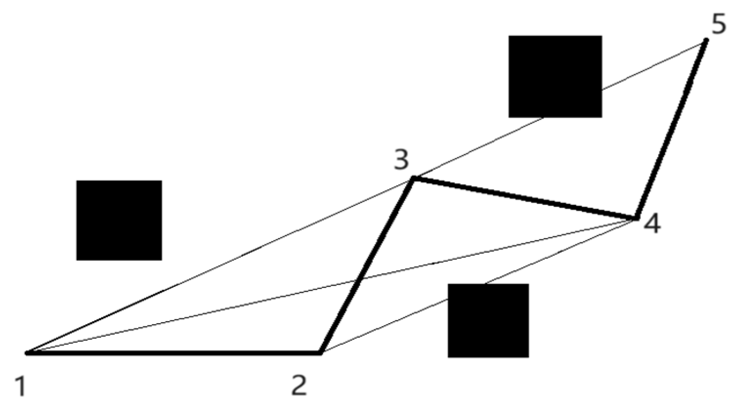
(2) Eliminate duplicate turning spots. The classic A* algorithm has more turning points, and the path is zigzag and discontinuous, resulting in discontinuity in the robot’s real traveling path and a lengthier moving path. As a result, preserving the key turning locations in the path while removing the superfluous turning points can significantly minimize the path’s turning length and shorten the search time, hence increasing efficiency[15]. Nodes 1 and 5 serve as the start and end points in the planned path and nodes 2, 3 and 4 are the inflection points set in the path planned by the traditional algorithm. The black square in the figure is the known obstacle and the black thick solid line is the path obtained from the traditional algorithm planning, which successfully avoids the obstacle and reaches the end point.
During path optimization, it is found that removing turning point 2 and following the route 13 directly reduces the path length, and the paths 2,4 and 3,5 are eliminated due to the presence of obstacles. Thus following the route 1,4,5 after removing turning points 2 and 3 at the same time is optimal, which reduces the path length and traveling time to a large extent.
Figure 3.
Schematic diagram of redundant turning point deletion.
2.3. Trajectory Circularization Process
The traditional A* algorithm obtains a path with a lot of turning points, which can wear out the tires of the robot and is not suitable for long time use with the robot. Thus the trajectory has to be smoothed to fit the robot’s operation[16]. Four path control nodes A, B, C, and D are obtained in the third-order Bussel curve, denotes the angle between node AB and the line where node BC is located, and denotes the angle between node BC and the line where node CD is located, and the equations of the third-order Bessel curve when is an acute angle are shown below:
When the path angle is obtuse, as shown in Figure 4, the result of optimizing the robot’s trajectory points E, G, and O. This trajectory consists of two identical third-order Bezier curves and the lines EG and OG, which get the curvature continuity, and the distance between E and O is found to be:
In the formula, are constants, , kmax is the maximum distance from any point on the curve to A or G.
3. Dynamic Window Approach
3.1. Motion Modelling of Mobile Robots
A well-liked approach for route planning, the dynamic window approach, models a robot’s movement at various rotational velocities and speeds in order to determine the optimal path for it. Before applying the dynamic window approach, the robot’s parameters must be recorded and the kinematic modeling must be completed[17]. Assuming that the mobile robot carries out a uniform linear motion during t time, this motion model can be expressed as:
denote the coordinate position of the robot, denotes the robot’s facing angle, denote the robot’s linear and angular velocities.
According to the motion model, we can simulate the motion of the robot under different velocities and angular velocities. This allows us to balance the advantages and disadvantages of each simulated path and ultimately select the optimal path for the robot’s navigation. By employing the dynamic window technique to select the best path within a given range of linear and rotational velocities, the robot may travel safely and effectively[18].
3.2. Velocity Sampling
The mobile robot operates within the constraints of its hardware and working environment. The maximum and minimum speeds at which it can operate can be expressed as follows:
During the path planning process, the robot’s acceleration and deceleration are controlled, thereby limiting the actual velocity changes. The maximum and minimum velocity range can be expressed as:
and represent the current velocity, and denote the maximum acceleration, and signify the maximum deceleration.
The speed range parameters can be configured according to the specific mobile robot and application requirements. During path planning, the robot’s speed is adjusted within this range to meet both safety and efficiency requirements. The robot travels on the intended path while adhering to the speed limitations by setting the minimum and maximum speed limits correctly. This keeps the robot moving within a restricted speed range.
A mobile robot must slow down to zero speed before it reaches an impediment in order to guarantee its safety while in operation. This restriction can be expressed in the following way:
indicates the distance of the robot from the obstacle.
3.3. Similar Day Clustering Results
The optimum speed group is chosen from the sampled speed data groups for local route planning, resulting in the final optimal path trajectory. This trajectory seeks to reach the target spot as smoothly as possible while properly avoiding obstacles in the lowest amount of time[19]. The evaluation function guiding this selection process is:
In this context, represents the robot’s azimuth and is used to calculate the angular deviation; denotes the velocity of the robot; and describes the distance between the robot’s current position and each point, calculating the distance from the target point. The three parameters, and are weighting coefficients, while is the smoothing coefficient.
3.4. Normalization Process
To avoid a biased representation of any specific evaluation metric in the overall evaluation function, it is essential to generalize the terms of the evaluation function prior to optimization.
Additionally, prior to optimization, the terms of the evaluation function need to be normalized. Regardless of variations in the initial scales or magnitudes of each component, this normalizing technique guarantees that each one contributes proportionately to the overall evaluation[20].
The trajectory that needs to be assessed first in Equations is the one corresponding to the current, while n represents the trajectory inside the dynamic window.
3.5. Optimization of the Dynamic Window Method
The traditional dynamic window method demonstrates effective obstacle avoidance capabilities in scenarios with known static obstacles. However, in situations where the path is cluttered with numerous obstacles, including both dynamic and static ones of unknown characteristics, the conventional algorithm’s limitations become apparent. These drawbacks include poor flexibility, longer obstacle avoidance paths, and significant turning angles, ultimately hindering the robot from reaching its intended destination[21].
3.5.1. Setting of Safety Distances
The traditional dynamic window method, which handles a relatively limited range of motion states, often struggles with significant deviations from the original planned path when encountering dynamic obstacles moving at various speeds. This results in excessive movement distances and large turning angles. By adjusting the path points to account for the safety distance between the robot and the obstacles, we can ensure the robot’s safety while optimizing the path.
When the robot encounters an obstacle moving in the opposite direction, as illustrated in Figure 5A, and the distance between the robot and the moving obstacle is less than the safe distance d, while the angle between the obstacle’s direction of motion and the robot’s planned path exceeds 45, the robot must wait until the dynamic obstacle clears the planned path before proceeding. During this waiting period, the robot will maintain a minimum distance of d from the moving obstacle in front of it.
When a robot hits an obstacle while traveling, the traditional algorithm normally proposes that it reverse course to avoid it. In actuality, the robot moves at a very slow pace, making it challenging to help it make the direction change. In certain situations, it can be wiser to follow the moving obstruction.
As illustrated in Figure 5B, the robot will stay on its current path, decrease its maximum speed, and make sure that it is at least d away from the moving obstacle when the distance between it and the robot is less than d and the angle β between the obstacle’s direction of movement and the robot’s planned path is less than 15°.
4. Fusion Algorithm
Taking into account the strengths and weaknesses of the two algorithms discussed in the previous section, we have decided to integrate the improved A* algorithm with the optimized dynamic window method. Although the enhanced A* algorithm is still a conventional global path planning technique, it is unable to satisfy complex environments’ dynamic obstacle avoidance needs. Real-time path planning for obstacle avoidance tasks in complicated environments is made possible by the dynamic windowing method. Nevertheless, when faced with multiple obstacles, it frequently becomes stuck in local optima and is unable to find the end goal location. We have chosen to combine the enhanced A* algorithm with the optimized dynamic window approach, taking into consideration the positive and negative aspects of the two methods covered in the preceding section. This fusion aims to design an evaluation function system that leverages global environmental information for comprehensive path planning.
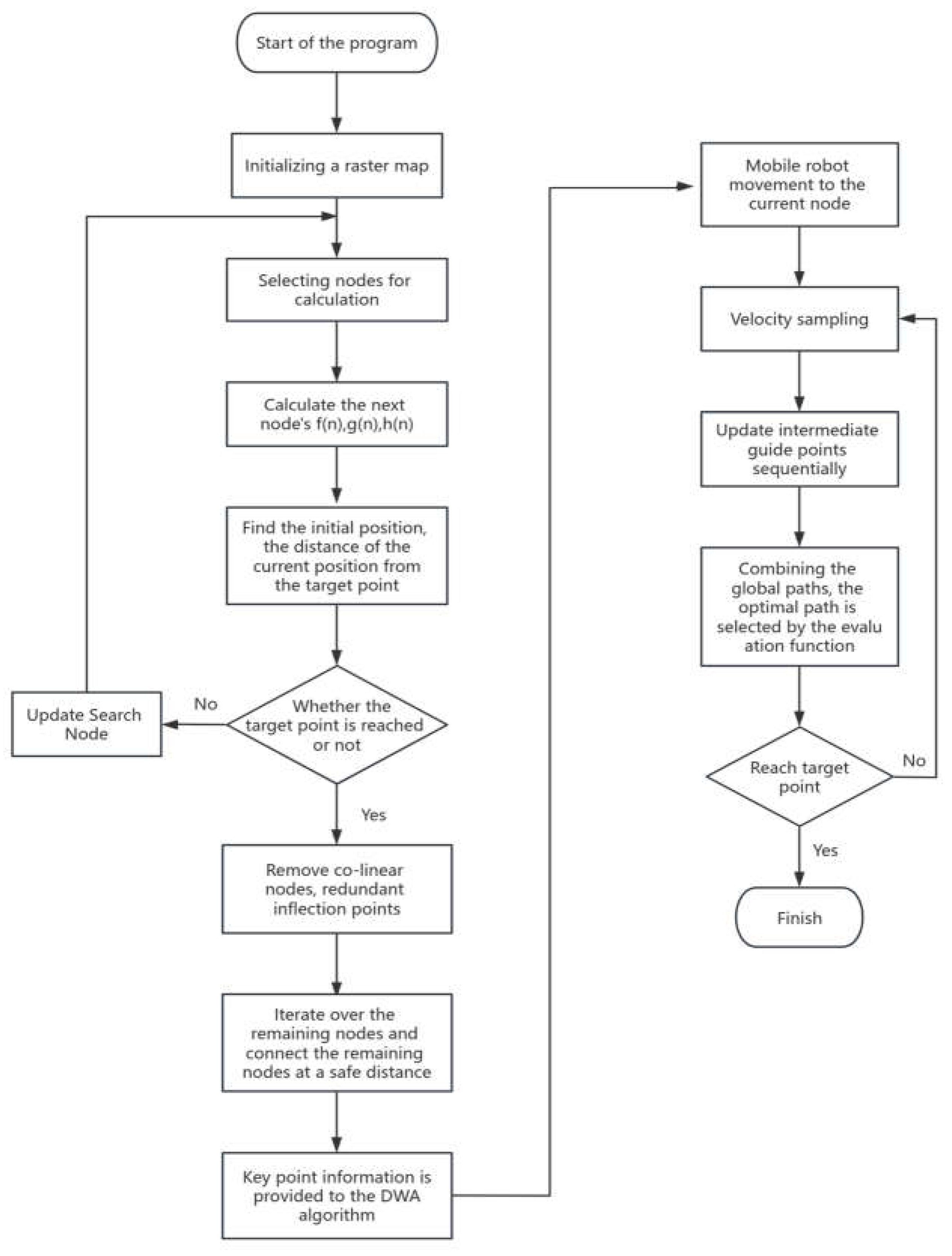
The flowchart below illustrates the proposed fusion algorithm.
Figure 6.
Flowchart of the fusion algorithm.
5. Simulation Experiment Verification
5.1. Simulation Verification of Improved A* Algorithm
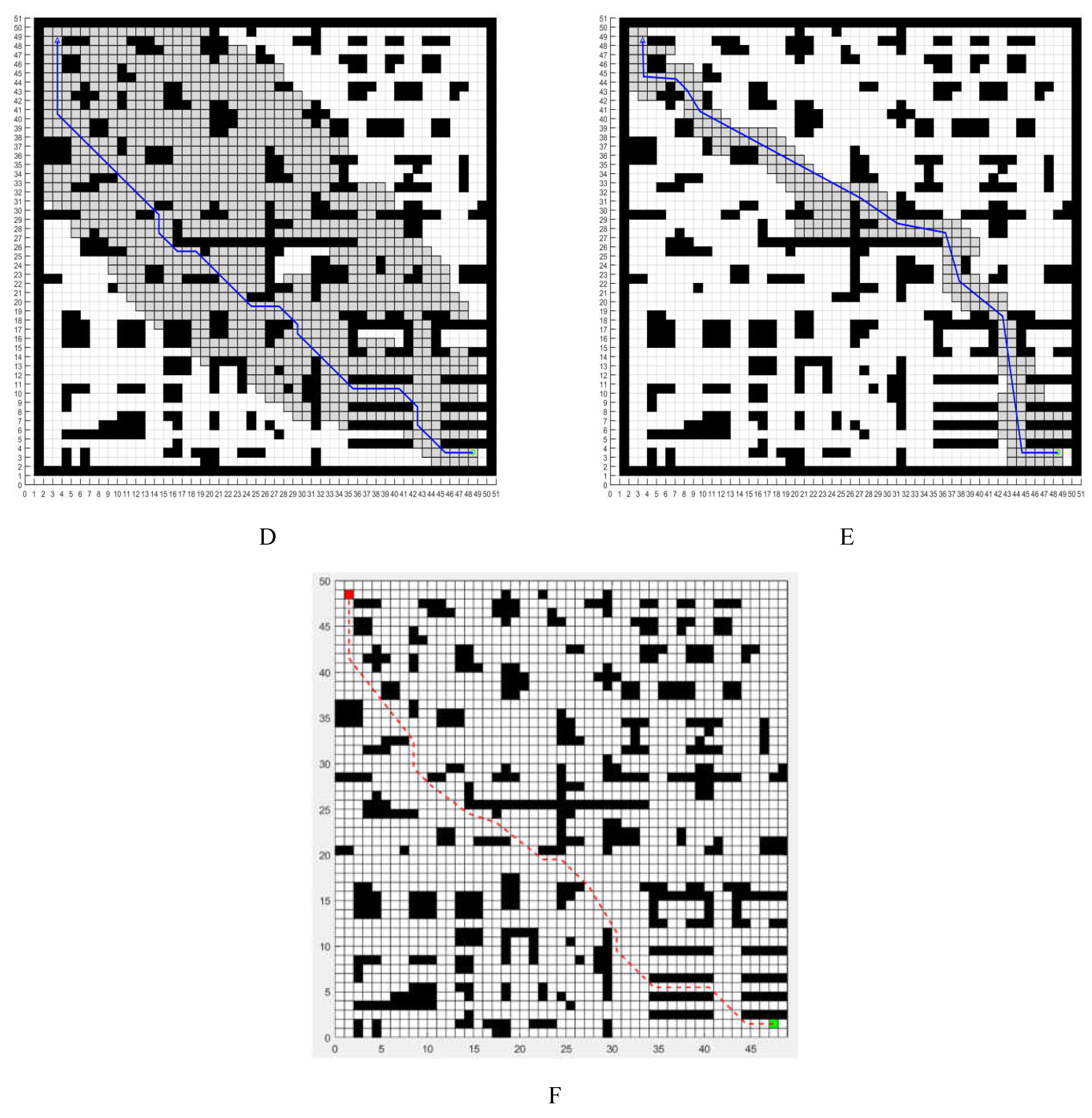
To evaluate the performance improvements of the enhanced algorithm, several simulation experiments will be conducted in various environments. Figure A and Figure D show the traditional A* algorithm, Figure B and Figure E show the improved A* algorithm. Figure C and F show the improved A* algorithm from literature 22 and will be compared to the improvements[22]. The shaded area is the pathfinding search cost of the different algorithms.
Figure 7.
Comparison of traditional A* and improved A* algorithms in different environments.

The following table shows the experimental results obtained after several repetitions of simulation experiments in the above two environments, and the following performance index parameters are compared:

Table 2.
Performance Analysis Comparison of Traditional A* Algorithm and Improved A* Algorithm.
| Planning time(/s) | Angle of divergence(/°) | Inflection | Planning node | Path length(/m) | |
| Figure A | 0.179 | 585.022 | 13 | 282 | 47.355 |
| Figure B | 0.104 | 123.203 | 6 | 140 | 41.399 |
| Figure C | 0.142 | 240.175 | 6 | 172 | 45.113 |
| Figure D | 0.366 | 790.255 | 14 | 546 | 76.965 |
| Figure E | 0.218 | 190.358 | 8 | 270 | 69.286 |
| Figure F | 0.244 | 486.355 | 10 | 312 | 74.847 |
It is evident from the above table’s comparison of several reference sets that the enhanced algorithm significantly reduces the path’s search range, greatly enhances its smoothness, and drastically reduces the excessive number of turning and planning nodes. It is clear from the search region shown by the shaded portion that the search cost has been much decreased, improving computing efficiency and avoiding the major drawback of the old methods’ inefficiency. The enhanced algorithm path is inherently silky smooth, which is more suitable for the robot’s operation and control. This fusion aims to design an evaluation function system that leverages global environmental information for comprehensive path planning[23].
5.2. Simulation Verification of DWA Algorithm Optimization
The dynamic window parameter indicators were set as follows: maximum speed 5m/s, maximum angular velocity 20°/s, rotational speed resolution 1°/s, acceleration 0.2m/s, and rotational acceleration 50°/s. The parameters in the evaluation function were set as follows: =0.05, =0.2, and =0.2, and the prediction time period was 3.0s. The parameters in the evaluation function are set as follows: =0.05, =0.2, =0.2, and the prediction time period is 3.0s.
In the Figure 8 below, the pink obstacles are static and the black obstacles are dynamic and will move in a certain direction without stopping. The cart starts at (0,0) and ends at (10,10).
Step 1, black dynamic obstacles emerged in the direction of the car this time. Based on the DWA algorithm’s before optimization, the car chose a safe distance. The vehicle then came to a stop to wait for the impediments to move, looked at them at the next operational moment, calculated their speed, and identified the next movement path moment.
Step 2, the car will now resume its intended course after entirely avoiding the dynamic impediments in front of it.
Step 3, the car detects the movement of the dynamic obstacle below, and judges whether the distance between itself and the obstacle meets the safety distance, and whether it needs to reduce the speed and wait for the movement of the dynamic obstacle.
Step 4, detected by the car, the car’s motion linear velocity, angular velocity and the initial distance from the car to meet the basic conditions of the passage, at this time the car successfully passed the obstacle bend.
Step 5, the cart slows down when it detects the motion of a dynamic obstacle close to the target position.
Step 6, after detecting a dynamic obstacle turning direction away from the cart, the cart moves to reach the target point.
5.3. Simulation Verification of the Fusion Algorithm
After the fusion of the improved algorithm with the dynamic window method, new gray static obstacles and yellow dynamic obstacles are added on the basis of the original full map path planning. Then multiple sets of repeated simulation experiments are conducted to verify the feasibility of the fusion algorithm to cope with various complex environments, and the performance parameters obtained from the experimental results are analyzed.
As shown in Figure 9, the improved A* algorithm is used for global path planning. When a new obstacle appears along the planned path, it poses a pathfinding challenge for the robot, preventing it from reaching the endpoint smoothly.
The fusion method adds three unknown gray static obstacles and three yellow dynamic obstacles in longitudinal motion, as Figure 10A illustrates. The robot then proceeds along its original intended path until the set random obstacles emerge. When the robot encounters the phased dynamic obstacles, it judges the positional relationship and maintains a safe distance, waits until the dynamic obstacles are far away from the planned route, and then re-moves according to the original planned route, and after encountering the static obstacles, it carries out random obstacle avoidance and then continues to move along the original planned route.
As shown in Figure 10B, the fusion algorithm is used to add isotropic dynamic obstacles and unknown three static obstacles, and the robot will follow the route planned by the improved A* algorithm before the appearance of the set gray random obstacles. When the robot appears throughout isotropic dynamic obstacles, it evaluates the positional relationship and determines to follow the obstacles. After that, it reduces its speed and maintains a safe distance from the obstacles at all times. It then waits patiently until the impediments are out of the way of the robot’s path before continuing on the predetermined course.
Based on the simulation diagrams presented above, it is evident that by introducing random gray obstacles, altering the trajectory of the yellow dynamic obstacles, and adjusting the robot’s path, the algorithm successfully enables the robot to navigate around obstacles in accordance with the prescribed requirements. Ultimately, the robot reaches the target point, thereby validating the feasibility of the fusion algorithm outlined in this paper.
Figure 11 compares the two sets of attitude angles and demonstrates that it is unacceptable to force the robot to reverse its direction of travel to avoid a dynamic barrier because of the setup’s restricted movement speed. Consequently, the robot chooses to follow the dynamic obstacle when it advances in the same direction as it and its angle of movement is less than 15. Otherwise, it maintains a safe distance from the obstacle. By lowering the amount of steering operations, this method frequently produces better results by reducing the likelihood of accidents. It also enables the robot to choose shorter paths and fewer nodes, which are closer to its actual motion curve.
Figure 11 and Figure 12 show how a robot may regularly change its orientation and velocity magnitude in a complex environment and still arrive at its destination with a rather smooth linear velocity. Thus, it realizes the path planning in complex environments and smoothly completes the random obstacle avoidance task.
6. Conclusions
In this paper, we propose a proposed path planning algorithm that combines the improved A* algorithm and the optimized dynamic window method. The search direction of the A* algorithm is reduced, redundant turning points and co-linear nodes are deleted, and a smooth optimal planning path is obtained after the optimization of the Bessel curve; the dynamic window method is optimized for a single motion state, and the safety distance is set to cope with obstacles with similar motion states as the robot, and the improved A* algorithm is fused with the optimized dynamic window method, so as to achieve obstacle avoidance at local locations facing random obstacles under the condition of satisfying the optimal curves in the globally planned path. The improved A* algorithm is integrated with the optimized dynamic window method, so as to achieve obstacle avoidance in the face of random obstacles at local positions while satisfying the optimal curve in the global planning path.
Compared with the traditional A* algorithm, the improved A* algorithm in this paper has a shortening improvement of about 3% in the path length, a significant reduction of about 40% in the operation length, and a reduction of about 50% in the search nodes and 75% in the search cost during the whole search process. As a result, the operational efficiency of the A* algorithm is greatly improved in the actual operation process. The number of turns, turning angle, and planning path curvature are all significantly reduced, illustrating that the modified A* method in the present investigation is productive.
The improved A* algorithm fused with the optimized dynamic window method proposed in this paper has the ability to cope with random obstacles on the basis of the globally planned path, which meets the requirements of collision-free pathfinding for robots. Following experimental testing, we may infer that the fusion approach is useful in some situations and warrants further investigation and application.
The research results in this paper can be applied to the path planning and random obstacle avoidance of mobile robots in complex environments, which has certain practical value. The subsequent research work can be based on the distribution of obstacles to adjust the proportionate weight of the heuristic function and evaluation function to adapt to the ability of path planning in different environments.
Author Contributions
All authors contributed to the study conception and design. The first draft of the manuscript was written by Ruilong Zong and all authors commented on previous versions of the manuscript. All authors read and approved the final manuscript. Ruilong Zong: Conceptualization, Methodology, Software Programming, Writing-Original Draft, Writing- Reviewing and Editing draft preparation, Visualization, Formal analysis, Software, Validation, Conceptualization. Jianhui Lin: Funding acquisition, Project administration, Supervision, Validation, Investigation, Writing-Reviewing
Statements & Declarations
The authors declare that no funds, grants, or other support were received during the preparation of this manuscript.
Consent to participate
Informed consent was obtained from all individual participants included in the study.
Consent to publish
The authors affirm that human research participants provided informed consent for publication of the images in all Figures.
Data availability statements
No datasets were generated or analysed during the current study.
Competing Interests
The authors have no relevant financial or non-financial interests to disclose.
References
- Liu, L.; Wang, X.; Yang, X.; Liu, H.; Li, J.; Wang, P. Path Planning Techniques for Mobile Robots: Review and Prospect. Expert Systems with Applications 2023, 227, 120254. [Google Scholar] [CrossRef]
- Liao, T.; Chen, F.; Wu, Y.; Zeng, H.; Ouyang, S.; Guan, J. Research on Path Planning with the Integration of Adaptive A-Star Algorithm and Improved Dynamic Window Approach. Electronics 2024, 13, 455. [Google Scholar] [CrossRef]
- Ju, C.; Luo, Q.; Yan, X. Path Planning Using Artificial Potential Field Method And A-Star Fusion Algorithm. In 2020 Global Reliability and Prognostics and Health Management (PHM-Shanghai); IEEE: Shanghai, China, 2020; pp. 1–7. [Google Scholar] [CrossRef]
- Xu, X.; Zeng, J.; Zhao, Y.; Li, X. Research on Global Path Planning Algorithm for Mobile Robots Based on Improved A*. Expert Systems with Applications 2024, 243, 122922. [Google Scholar] [CrossRef]
- Lai, R.; Wu, Z.; Liu, X.; Zeng, N. Fusion Algorithm of the Improved A* Algorithm and Segmented Bézier Curves for the Path Planning of Mobile Robots. Sustainability 2023, 15, 2483. [Google Scholar] [CrossRef]
- Yi, C.; Hongtu, X. Global Dynamic Path Planning Based on Fusion of Improved A* Algorithm and Morphin Algorithm. In 2019 Chinese Control And Decision Conference (CCDC); IEEE: Nanchang, China, 2019; pp. 6191–6196. [Google Scholar] [CrossRef]
- Yin, X.; Dong, W.; Wang, X.; Yu, Y.; Yao, D. Route Planning of Mobile Robot Based on Improved RRT Star and TEB Algorithm. Sci Rep 2024, 14, 8942. [Google Scholar] [CrossRef] [PubMed]
- Liu, Y.; Wang, C.; Wu, H.; Wei, Y. Mobile Robot Path Planning Based on Kinematically Constrained A-Star Algorithm and DWA Fusion Algorithm. Mathematics 2023, 11, 4552. [Google Scholar] [CrossRef]
- Xu, D.; Yang, J.; Zhou, X.; Xu, H. Hybrid Path Planning Method for USV Using Bidirectional A* and Improved DWA Considering the Manoeuvrability and COLREGs. Ocean Engineering 2024, 298, 117210. [Google Scholar] [CrossRef]
- Deng, W.; Zhang, L.; Zhou, X.; Zhou, Y.; Sun, Y.; Zhu, W.; Chen, H.; Deng, W.; Chen, H.; Zhao, H. Multi-Strategy Particle Swarm and Ant Colony Hybrid Optimization for Airport Taxiway Planning Problem. Information Sciences 2022, 612, 576–593. [Google Scholar] [CrossRef]
- Zhenyang, X.; Wei, Y. Mobile Robot Path Planning Based on Fusion of Improved A* Algorithm and Adaptive DWA Algorithm. J. Phys.: Conf. Ser. 2022, 2330, 012003. [Google Scholar] [CrossRef]
- Mohanraj, T.; Dinesh, T.; Guruchandhramavli, B.; Sanjai, S.; Sheshadhri, B. Mobile Robot Path Planning and Obstacle Avoidance Using Hybrid Algorithm. Int. j. inf. tecnol. 2023, 15, 4481–4490. [Google Scholar] [CrossRef]
- Liao-Guocheng; Wu-Yajuan. Improved Robot Path Planning with A* and DWA Fusion. In 2023 7th International Conference on Automation, Control and Robots (ICACR); IEEE: Kuala Lumpur, Malaysia, 2023; pp. 14–19. [Google Scholar] [CrossRef]
- Wang, T.; Li, A.; Guo, D.; Du, G.; He, W. Global Dynamic Path Planning of AGV Based on Fusion of Improved A* Algorithm and Dynamic Window Method. Sensors 2024, 24, 2011. [Google Scholar] [CrossRef] [PubMed]
- Yu, M.; Luo, Q.; Wang, H.; Lai, Y. Electric Logistics Vehicle Path Planning Based on the Fusion of the Improved A-Star Algorithm and Dynamic Window Approach. WEVJ 2023, 14, 213. [Google Scholar] [CrossRef]
- Fransen, K.; Van Eekelen, J. Efficient Path Planning for Automated Guided Vehicles Using A* (Astar) Algorithm Incorporating Turning Costs in Search Heuristic. International Journal of Production Research 2023, 61, 707–725. [Google Scholar] [CrossRef]
- Liu, H.; Zhang, Y. ASL-DWA: An Improved A-Star Algorithm for Indoor Cleaning Robots. IEEE Access 2022, 10, 99498–99515. [Google Scholar] [CrossRef]
- Liu, J.; Yang, J.; Liu, H.; Tian, X.; Gao, M. An Improved Ant Colony Algorithm for Robot Path Planning. Soft Comput 2017, 21, 5829–5839. [Google Scholar] [CrossRef]
- Zhang, M.; Li, X.; Wang, L.; Jin, L.; Wang, S. A Path Planning System for Orchard Mower Based on Improved A* Algorithm. Agronomy 2024, 14, 391. [Google Scholar] [CrossRef]
- Huang, Y.; Ding, H.; Zhang, Y.; Wang, H.; Cao, D.; Xu, N.; Hu, C. A Motion Planning and Tracking Framework for Autonomous Vehicles Based on Artificial Potential Field-Elaborated Resistance Network (APFE-RN) Approach.
- Gao, H.; Ma, Z.; Zhao, Y. A Fusion Approach for Mobile Robot Path Planning Based on Improved A* Algorithm and Adaptive Dynamic Window Approach. In 2021 IEEE 4th International Conference on Electronics Technology (ICET); IEEE: Chengdu, China, 2021; pp. 882–886. [Google Scholar] [CrossRef]
- Zhang, B.; Cao, J.; Li, X.; Chen, W.; Zheng, X.; Zhang, Y.; Song, Y. Minimum Dose Walking Path Planning in a Nuclear Radiation Environment Based on a Modified A* Algorithm. Annals of Nuclear Energy 2024, 206, 110629. [Google Scholar] [CrossRef]
- Li, J.; Ji, M.; Liu, L.; Liu, Z.; Zheng, X.; Li, S. “Fusion of Improved A* Algorithm and Dynamic Window Approach for Path Planning, 2022 China Automation Congress (CAC), Xiamen, China, 2022, pp. 390–394. [CrossRef]
Figure 1.
Eight-Neighborhood Search Methods.
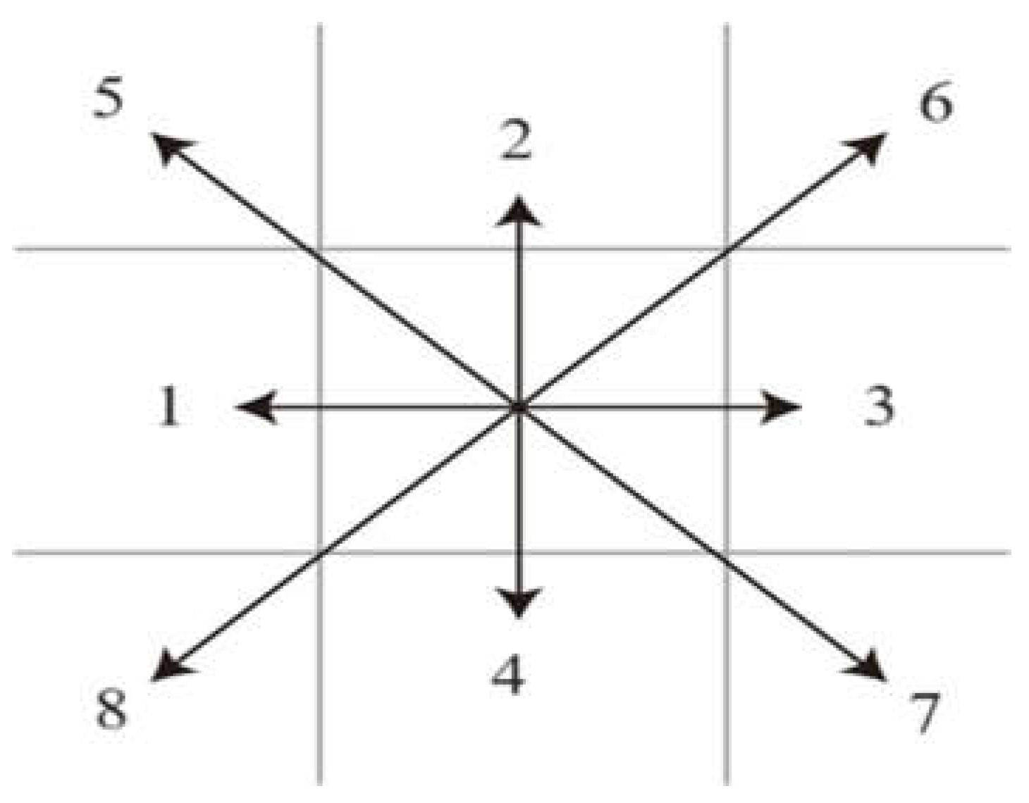
Figure 2.
Common Line Node Deletion Schematic.
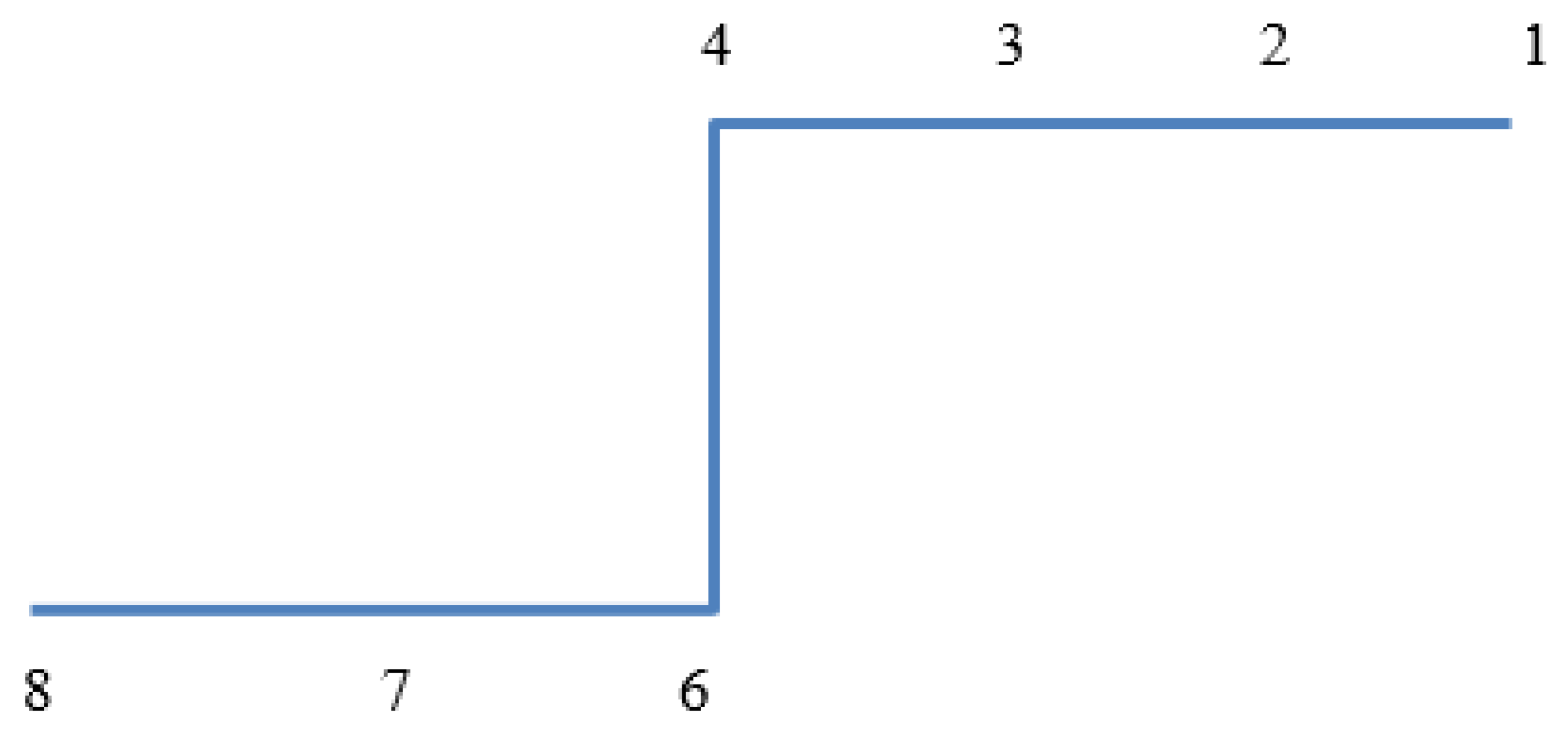
Figure 4.
Trajectory circularization processing schematic.
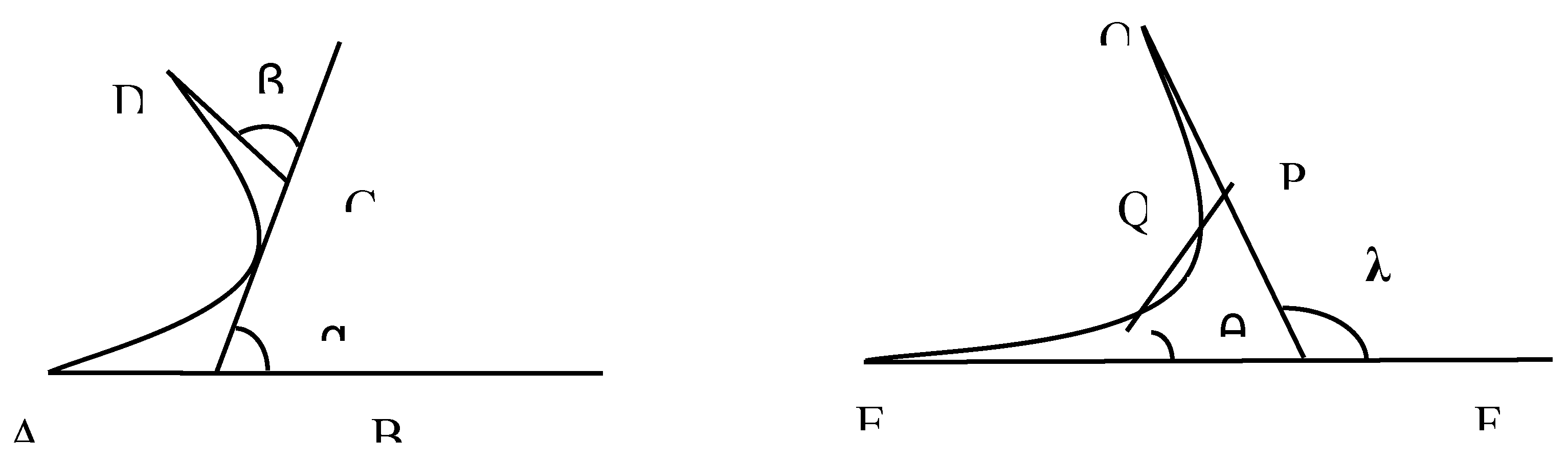
Figure 5.
Safety Distance Setting Schematic.
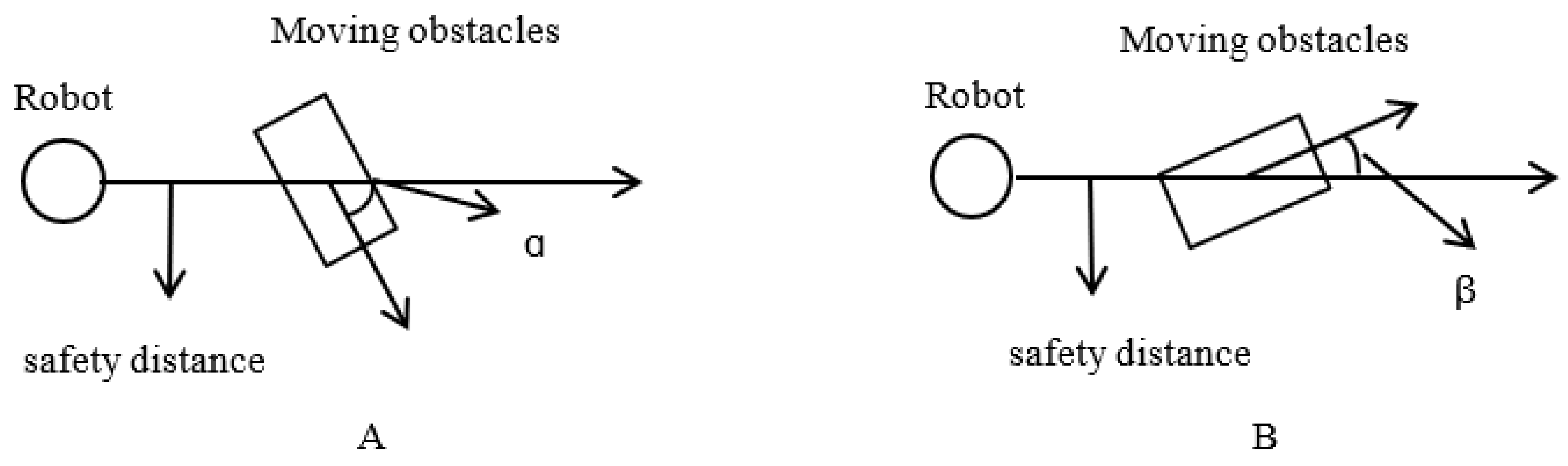
Figure 8.
Optimization Simulation Verification of Dynamic Window Method.
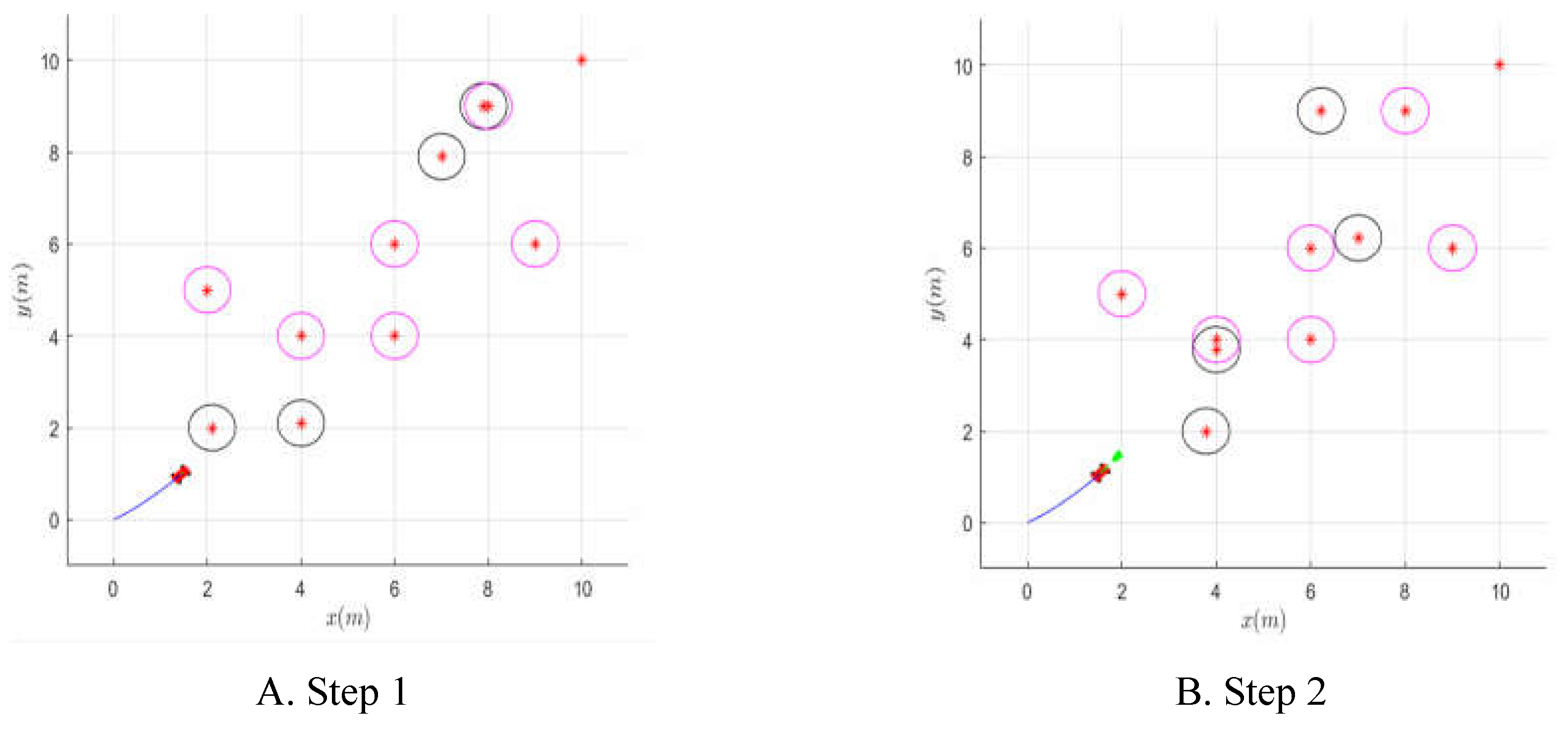
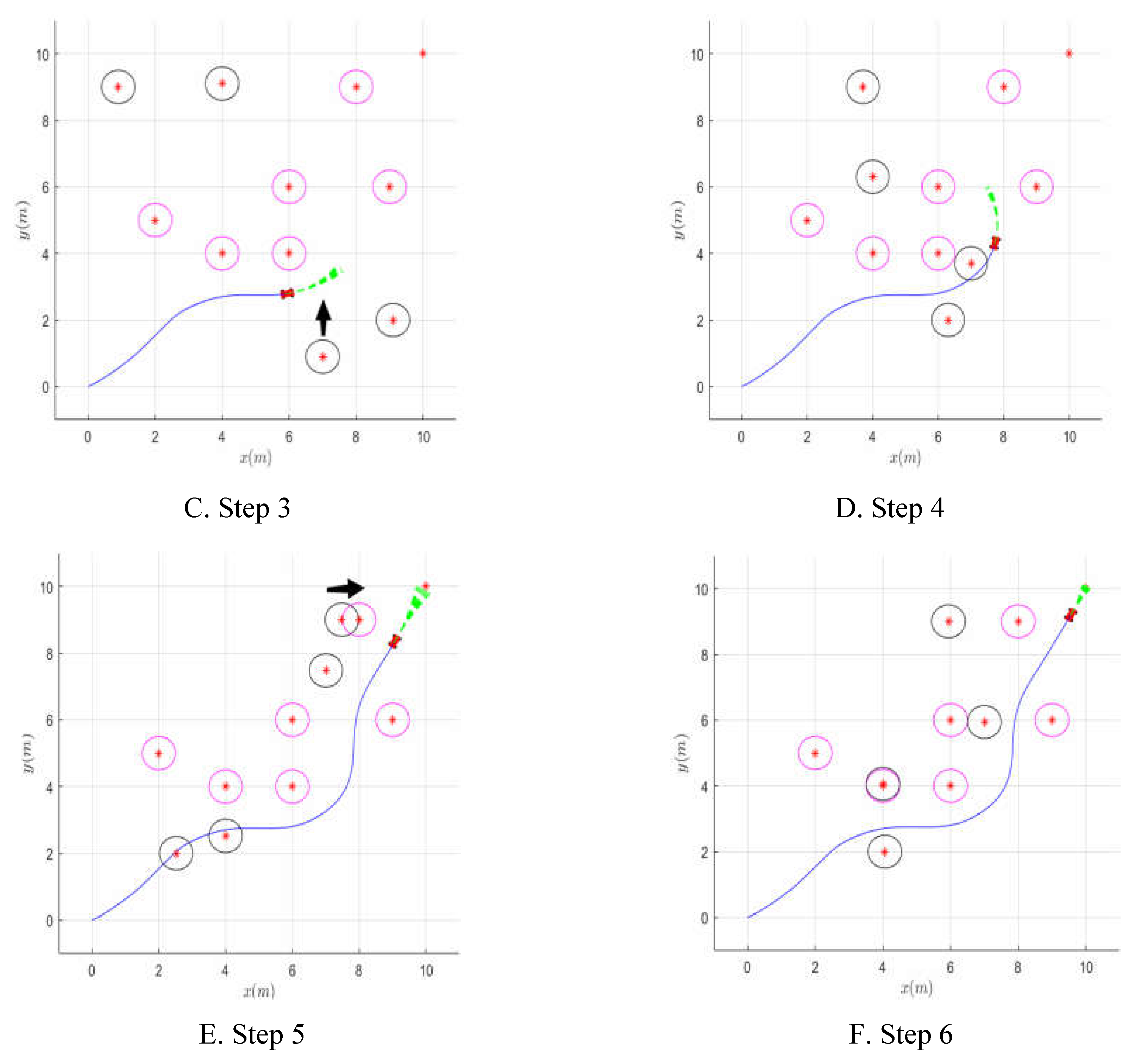
Figure 9.
Optimization Simulation Verification of Dynamic Window Method.
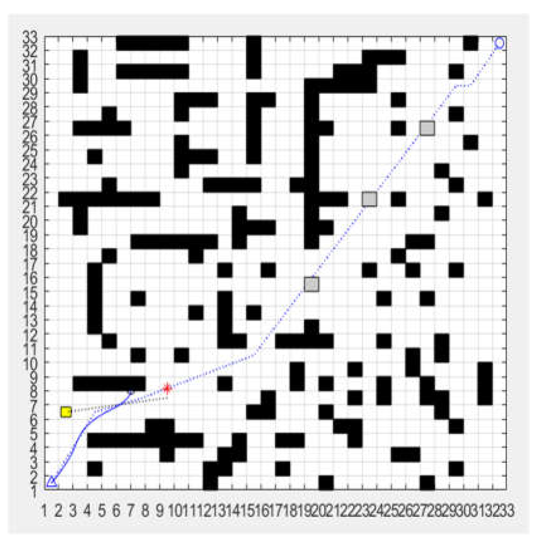
Figure 10.
Simulation validation plot of the fusion algorithm facing dynamic obstacles in different directions.
Figure 10.
Simulation validation plot of the fusion algorithm facing dynamic obstacles in different directions.

Figure 11.
Attitude Angle Chart Comparison.
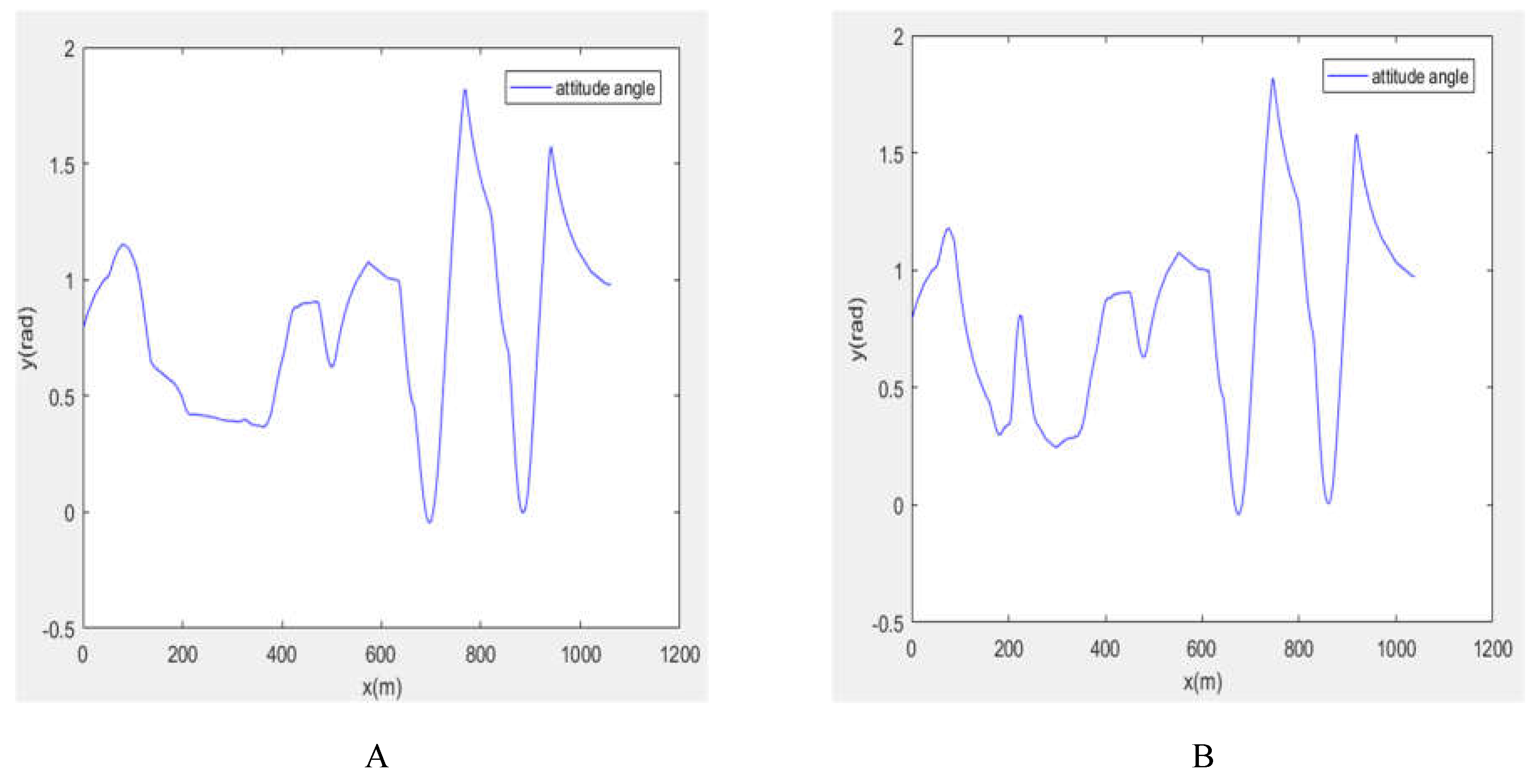
Figure 12.
Comparison chart of linear and angular speeds.
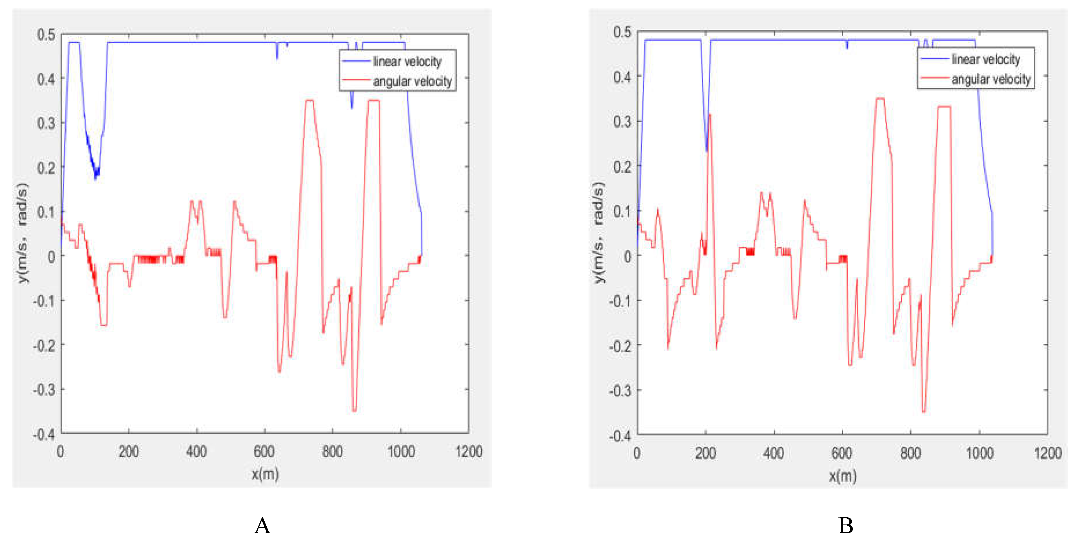
Table 1.
Correspondence table between clamp angle α and selection direction.
| α | Direction of reservations | Direction of Abandonment |
| [337.5°,360°)∪[0°,22.5°) | 12356 | 478 |
| [22.5°,67.5°) | 23567 | 148 |
| [67.5°,112.5°) | 23467 | 158 |
| [112.5°,157.5°) | 34678 | 125 |
| [157.5°,202.5°) | 13478 | 256 |
| [202.5°,247.5°) | 14578 | 236 |
| [247.5°,292.5°) | 12458 | 367 |
| [292.5°,337.5°) | 12568 | 347 |
Disclaimer/Publisher’s Note: The statements, opinions and data contained in all publications are solely those of the individual author(s) and contributor(s) and not of MDPI and/or the editor(s). MDPI and/or the editor(s) disclaim responsibility for any injury to people or property resulting from any ideas, methods, instructions or products referred to in the content. |
© 2025 by the authors. Licensee MDPI, Basel, Switzerland. This article is an open access article distributed under the terms and conditions of the Creative Commons Attribution (CC BY) license (http://creativecommons.org/licenses/by/4.0/).
Copyright: This open access article is published under a Creative Commons CC BY 4.0 license, which permit the free download, distribution, and reuse, provided that the author and preprint are cited in any reuse.


