Submitted:
02 January 2025
Posted:
03 January 2025
You are already at the latest version
Abstract
The purpose of this study is to explore the feasibility and effectiveness of Fiber Bragg Grating optical sensors (FBG sensors) in geotechnical engineering applications, both in controlled laboratory settings and in real-world field environments. Specifically, the study aims to evaluate the sensors' performance in monitoring key geotechnical parameters—such as strain, temperature and acceleration—under various loading conditions, including static, dynamic, seismic, and centrifuge loads. By assessing FBG sensors across these diverse conditions, the study seeks to determine their potential for improving the accuracy, safety, and reliability of geotechnical monitoring systems. Within this framework, the application of optical fibers was investigated using the one-degree-of-freedom shaking table at the National Technical University of Athens, with the goal of evaluating the sensors' performance during seismic loading. This investigation aimed to provide insights into the behavior of geotechnical physical models under seismic conditions, allowing conclusions to be drawn about the reliability and accuracy of optical fiber sensors in capturing dynamic responses during earthquake simulations. Furthermore, several physical models were constructed and tested using the drum geotechnical centrifuge at ETH Zurich. During testing, optical fiber strain recordings were made possible as gravitational acceleration was increased up to 100g and impact loading scenarios were included. The optical fiber sensors successfully captured the loading conditions, and the recorded data reflected the anticipated behavior of the models, demonstrating the sensors' effectiveness in monitoring geotechnical responses under extreme loading scenarios. Following the laboratory investigation, optical fibers were installed at the Acropolis of Athens Perimeter Wall (Circuit Wall) to record strain, acceleration, and temperature in real-time and remotely. The installation of this monitoring system posed significant challenges due to the limitations of the archaeological site, requiring careful planning and execution. Despite these difficulties, data was successfully gathered over an extended period of two years, providing insights into the structural behavior of the historic site under various environmental and loading conditions. Regarding the aforementioned applications, the test setups and monitoring schemes are presented in detail. This includes an overview of the types of sensors used, the coating materials, and the methods employed for integrating the sensors into both the experimental models and the Acropolis Hill. Additionally, the data gathering techniques are discussed, along with any technical issues that arose during the process and the proposed solutions. Finally, indicative recordings are provided, along with their interpretation. The results align with expectations, demonstrating the effectiveness of optical fibers in various applications and underscoring their vast potential in geotechnical engineering. This highlights the numerous opportunities for incorporating optical fiber sensors in future projects, reinforcing their role as valuable tools for monitoring and assessing structural integrity.
Keywords:
FBG Sensors
; Geotechnical Engineering
; Acropolis of Athens
; Seismic Loading
; Scaled Physical Modelling
; Optical Fibre Sensors
; Field Implementations
; Laboratory Testing
; Geotechnical Centrifuge
1. Introduction
In the modern era there is a growing need for rapid acquisition of information related to the response of structures under various loading conditions, such as earth pressures, dead and self-weight loadings and due to geo-environmental and geophysical hazards, including seismic events. Natural phenomena and hazards typically occur suddenly and often with significant intensity, potentially leading to structural issues or even total failures. Structural monitoring plays a crucial role in hazard assessment (i.e., evaluating the loading conditions) and in the early detection of damage or impending failures, contributing to improved risk management and overall structural safety (Kapogianni, 2023). Real-time data acquisition enables the development of early warning systems that activate when predefined limits are exceeded, allowing for automatic system control and enhanced responsiveness
More specifically, sensors and monitoring devices can be employed to assess the structural response to both static and dynamic loadings in laboratory testing and in field applications (Pelekanos et al., 2017). These systems are utilized in projects of various scales, from infrastructure works to, more recently, Cultural Heritage Sites (Kapogianni et al., 2019). The selection of an appropriate monitoring scheme is tailored to each site or project, taking into account factors such as sensor type, installation locations, and quantity. These decisions depend on the scale of the project and its specific characteristics. Additionally, the scheme is influenced by the importance of the site and the expected loading scenarios. For example, a smaller, moderately significant engineering project in an area with low or medium anticipated hazards would require fewer sensors compared to a large-scale, high-priority site located in a high-risk hazard zone.
In civil engineering projects, Brillouin and Bragg Grating optical fiber sensors are widely used for monitoring the structural integrity and measuring parameters like strain, stress, and temperature (Soga et al., 2015, Minardo et al., 2021). These sensors offer high precision, resistance to mechanical stress, and signal multiplexing at a relatively low cost. A key advantage is their portability, allowing them to be easily installed at various positions to monitor hazards (i.e., loading conditions) and assess structural responses or distress in critical areas. Brillouin optical fibers are ideal for distributed sensing across large structures like bridges and pipelines, providing long-range strain and temperature monitoring (Kechavarzi et al., 2016, Iten et al., 2011). In contrast, Bragg Grating optical fibers offer precise, localized measurements, making them suitable for critical points during laboratory testing and/or in the field. In this study, the use of Fiber Bragg Grating, (FBG) sensors is demonstrated both in laboratory settings—featuring various test setups—and in field applications, with a focus on the Athenian Acropolis Hill, highlighting the wide range of potential applications these sensors offer.
2. Structural Monitoring and Seismic Loading
Earthquakes and seismic events generate dynamic stresses and deformations in critical infrastructure like buildings, slopes, pipelines, bridges, tunnels, and dams. Traditional monitoring systems often struggle with limited coverage, real-time data acquisition, and durability under harsh conditions. Over the last decades optical fiber sensors have been used for monitoring structures and environments under seismic loading (Bado & Casas, 2021). For example, optical fiber sensors have been utilized to monitor geotechnical slopes, providing precise, continuous, real-time data. These slopes, especially in regions with unstable geology or active construction, are vulnerable to landslides, erosion, and deformation. While tools such as inclinometers and piezometers are useful, optical fiber sensors offer superior spatial resolution and long-term reliability. In pipeline monitoring, optical fiber sensors play also a crucial role by delivering continuous data and early failure detection. Their ability to monitor strain, temperature, and seismic activity over extended distances makes them indispensable for maintaining pipeline integrity and preventing costly, hazardous incidents. Given the rising demand for secure, efficient pipeline systems, optical fiber technology is poised for further expansion in infrastructure monitoring. Similarly, optical fiber sensors are vital in overseeing reinforced slopes, which stabilize embankments, cuttings, and landslide-prone slopes in geotechnical engineering. These slopes are commonly reinforced with materials such as geotextiles, geogrids, soil nails, or retaining walls to improve stability. Monitoring their performance is essential to maintaining long-term structural integrity, especially in areas exposed to external stressors like heavy rainfall, seismic events, or ground subsidence.
In the current study, optical fiber sensors were deployed at the laboratory shaking table of the National Technical University of Athens to assess their performance under dynamic and seismic loadings (Kapogianni et al., 2019). Specifically, strain and acceleration sensors were attached to various scaled-down physical models to record variations as loading increased. The following section presents the test setup and provides representative recordings. Figure 1 illustrates the laboratory equipment, which includes: a) a single-degree-of-freedom force generator, used to create seismic motion by converting electrical signals into kinetic energy; b) an amplifier that boosts the low-power supply signal to one capable of directly driving the shaker; c) a data acquisition card with analog and digital inputs/outputs, facilitating the connection between the computer and the generator, as well as controlling the shaking table’s frequency and magnitude; d) custom LabView software developed to operate the system; e) an interrogator for data collection; and f) the optical fiber sensors used in the experiments.
Fiber Bragg Grating (FBG) sensors (Figure 2), equipped with different coatings, adhesives, and restraint configurations, were embedded in various geotechnical models constructed within a transparent, watertight box. The following section outlines four representative tests that showcase the performance of these optical fiber sensors in a controlled laboratory environment. Detailed descriptions of each model's geometric characteristics, as well as the acceleration levels applied via the shaking table or force generator, are provided. The strain measurements captured by the optical fiber sensors are presented, alongside a comparison of observed failure mechanisms with those predicted by numerical simulations and finite element stress analysis.
During Test No. 1, a scaled sand slope model was constructed within the transparent, watertight box mounted on the earthquake simulator (Figure 3). An optical fiber sensor was embedded at a height of 8.5 cm above the base. A small, predetermined amount of water was incorporated during construction, with a water level set at 6 cm to examine failure mechanisms in the presence of water. The maximum applied acceleration during the test reached 3.8 m/s². A digital camera, positioned on the earthquake simulator platform, captured the entire failure sequence (Figure 4). As anticipated, erosion/scouring occurred at the slope’s base due to water movement. Additionally, a diagonal tensile crack developed at the top of the model, signaling strain localization, a typical pre-failure behavior in granular slopes. The crack propagated, leading to the sliding of a significant soil block and the complete failure of the model.
The failure of the scaled sand slope model during Test No. 1 can be attributed to the combined effects of dynamic loading, water-induced instability, and the inherent properties of granular materials. The dynamic acceleration of 3.8 m/s² from the earthquake simulator generated cyclic shear stresses, leading to particle rearrangement and a reduction in shear strength. The presence of water at a 6 cm level introduced hydrostatic pressure, reducing the effective stress and frictional resistance within the slope. This condition facilitated erosion at the slope base due to water movement, undermining stability and initiating failure. Simultaneously, the cyclic loading caused strain localization, manifesting as a diagonal tensile crack near the slope’s top, a common precursor to failure in granular slopes. The propagation of this crack formed a failure plane, resulting in the sliding of a significant soil block and the complete collapse of the model.
In Figure 5 (left), strain recordings from the optical fiber sensor are displayed as the slope model was subjected to seismic loading. As expected, strain increased during the applied seismic load, with the highest strain values occurring just before the slope's failure. Notably, in the approximately 50-second period leading up to failure, strain levels remained relatively low, reaching up to 180 μstrain. However, as the crack at the top of the slope widened, strain levels sharply increased, peaking at 980 μstrain during the slope's collapse. Specifically, Curve A in the diagram shows a small gradual strain increase during seismic loading, culminating in a maximum point (Peak A), which corresponds to the initiation of the crack. As the crack expanded further, a second much higher peak (Peak B) was recorded just before the large soil mass slid, signaling total failure. The final segment of the diagram (Curve B) shows significantly lower strain values, indicating that the soil mass had already failed. The model’s behavior and failure mechanism aligned with expectations based on the literature and were accurately captured by the optical fiber sensor strain recordings.
More specifically, strain recordings from the optical fiber sensor capture the progressive deformation of the slope model under seismic loading. Initially, strain values increased gradually as the slope experienced seismic forces, remaining relatively low (up to 180 μstrain) as the material stayed within its elastic range. As the seismic load continued, strain levels began to rise sharply with the initiation of a crack at the top of the slope, reaching Peak A, corresponding to the onset of strain localization. As the crack expanded further, a significant increase in strain was observed, peaking at Peak B, just before the soil mass slid, indicating a transition from elastic to plastic deformation and signaling imminent failure. After the collapse, the strain values decreased significantly, as shown in Curve B, reflecting the failure of the soil mass, which no longer responded to the seismic loading. These recordings provide clear evidence of the failure mechanism and demonstrate the effectiveness of optical fiber sensors in capturing the geotechnical behavior of the model under seismic conditions.
A second model with similar geometric characteristics but subjected to lower acceleration levels, up to 2.8 m/s², was constructed and tested (Test No. 2) and the strain variations recorded by the optical fiber sensor are shown in Figure 5 (right). The lower strain levels observed in Test No. 2, as recorded by the optical fiber sensor, are directly related to the reduced seismic acceleration of 2.8 m/s² compared to 3.8 m/s² in Test No. 1. The sensor measurements clearly show a decrease in maximum strain values, reflecting the lower stress and deformation in the model due to the reduced acceleration. This behavior is consistent with geotechnical principles, where smaller seismic forces result in lower strain responses. The optical fiber data effectively demonstrate how variations in seismic loading influence the mechanical behavior of the slope, highlighting the sensor's ability to capture such differences under different seismic conditions.
Additionally, two numerical models were developed to examine the expected theoretical behavior of the slope models. Figure 6 (left) presents the results obtained using the Bishop Analysis method, while Figure 6 (right) displays a numerical model created and analyzed through the Finite Element Stress Analysis Method. The loading conditions for these models were similar to those imposed during Test No. 2, and the expected failure mechanisms closely align with the actual failure modes observed in the physical modeling tests. The Safety Factor (SF) and Strength Reduction Factor (SRF) values being below 1 in the numerical models are consistent with the expected failure behavior of the slope under the specified loading conditions. In the Bishop Analysis, an SF below 1 indicates that the slope is unstable and likely to fail, which aligns with the physical test results, where the model collapsed under seismic loading. Similarly, the Finite Element Method (FEM) model, with an SRF below 1, suggests that the material strength was insufficient to prevent failure under the applied stresses, matching the actual failure observed in Test No. 2. Both numerical methods accurately predicted the slope's instability, confirming their effectiveness in modeling the expected failure mechanisms.
In Test No. 3, an optical fiber sensor was attached to a scaled pipe placed at the estimated critical point of the slope, where higher stress concentrations were anticipated. This setup was designed to simulate the use of pipes as reinforcement elements within the slope, where they serve to support the soil, redistribute pressure, and reduce strain. The purpose of this test was to evaluate how the presence of the reinforcing pipe influences the stress distribution and deformation behavior of the slope. By monitoring the strain at this critical point, the test aimed to provide insights into the effectiveness of using pipes for slope reinforcement, modeling the interaction between the reinforcement system and the surrounding soil under dynamic loading conditions. More specifically, a maximum seismic loading of 4 m/s² was applied and the water level was set at 4cm. Figure 7 provides a side view of the slope model, with the embedded scaled pipe, Figure 8 shows the model's deformation during seismic loading, and Figure 9 displays the corresponding strain recordings. As observed in Figure 8, seismic loading caused visible scouring at the base of the slope, as well as shear initiation at the pre-existing tensile crack at the top of the slope. Furthermore, it can be noted in Figure 9 that strains observed during this test were significantly smaller than in previous tests (i.e. No. 1 and No. 2). This is both logical and expected, as the presence of the scaled pipe acts as soil reinforcement, increasing its overall stability. Despite this, the failure mechanism mirrored that of the earlier tests. Finally, post-test inspection detected visible deformation at the pipeline’s critical point, confirming the sensor’s ability to accurately capture the structural response.
Test No. 4 involved a reinforced vertical slope model, with two optical fiber sensors embedded within two geotextile reinforcement layers, with a maximum applied acceleration of 4 m/s². Figure 10 illustrates the reinforced model, providing both a side view of its structure and the corresponding failure mechanism. The structural response of this model differed significantly from the unreinforced slopes tested earlier. As shown in Figure 11, the failure was a localized shear failure rather than a complete or catastrophic collapse, which is typical for reinforced slopes. It was primarily confined to the slope's face, and the strain levels recorded by the optical fiber sensors were significantly lower than in previous tests, as anticipated. This test underscores the critical role of reinforcement layers in geotechnical slopes. The reinforcement allowed for the successful construction of a vertical slope model, and despite the high acceleration, strain levels remained minimal. Additionally, the failure was localized to specific areas of the model, with no overall collapse. These results highlight the effectiveness of reinforcement in maintaining slope stability under seismic loading, as also confirmed by the optical fiber sensor recordings.
3. Optical Fiber Sensors and Enhanced Gravity-Centrifuge Loading
Optical fiber sensors were deployed at the drum geotechnical centrifuge of ETH Zurich (Springman et al., 2001), enabling strain recordings during centrifuge load increases and impact loading scenarios. Geotechnical centrifuges are widely used to experimentally investigate scaled-down geotechnical structures by applying a gravitational field "n" times greater than Earth's gravity. This scaling is crucial, as the dominant forces affecting soil structure behavior are gravity-driven, making small-scale testing under normal gravity insufficient (Pokrovsky and Fedorov, 1936; Schofield, 1980). The optical fiber sensors were affixed to the scaled physical models with minimal coating materials to prevent interference with the model behavior, ensuring accurate strain variation measurements. The primary objective of this application was to assess the performance of the sensors within the centrifuge environment and to study the behavior of the scaled models under varying loading conditions.
Several wrap-around reinforced sand slope models were built with the same geometry inside a strong box, incorporating uniformly spaced reinforcement materials to simulate reinforced soil slopes as can be seen in Figure 12 (Kapogianni et al., 2017). Textile-embedded optical fiber strain sensors were strategically attached on the reinforcement layers to monitor strain development during various loading scenarios. A transparent, colorless liquid photopolymer glue was used to affix the sensors to the scaled reinforcement layers. The sensors were embedded using a two-component, fast-curing adhesive, comprising a liquid and a powder, which created fixed boundaries, preventing sensor slippage and ensuring accurate strain measurements throughout the tests. The soil material used for the models was a fine-grained uniform sand from the west coast of Australia (Nater, 2005).
Each optical fiber had an individual/unique initial wavelength, and wavelength variations were recorded as g-levels increased. A portable interrogator, positioned along the centrifuge’s axis inside a rigid box to shield it from high g-forces, was used for data collection (Figure 13). The sensors were connected in series via a splicing device, and data acquisition was managed through custom LabView software. This configuration enabled simultaneous strain measurements every second, due to the distinct initial wavelengths of the sensors. No temperature variations were observed during the study. Impact loading was simulated using a steel block to represent a boulder falling onto the slope models. Impact loading was investigated and a model block made of steel was used to simulate a boulder falling on the slope models. The boulder was attached to a magnet on the tool platform which was rotating together with the drum. The purpose of the electro-magnet was to hold the block during the test to release it at the desirable moment. A guiding tube was used along the fall path of the block to ensure orthogonal contact between the block and the surface of the slope and also to keep the block in ng field to achieve high energy levels (Chikatamarla et al., 2006). Vibrations generated by the impact were measured by two Brüel & Kjær accelerometers. The maximum acceleration recorded for the model boulder during impact reached 9.7 m/s², subjecting the models to forces of up to 100 g. Additionally, a digital camera was placed on the side of the models and recorded digital images during the loading events, in order to perform PIV Analysis via GeoPIV (Kapogianni et al., 2010).
The wavelength changes recorded by the sensors during the loading events were converted into strain using the following equation: Δε=(Δλ-Κs*ΔΤ)/Κε, where: Δε represents the strain change, Δλ is the wavelength change, Κs is equal to 11.2 pm/°C, reflecting the temperature sensitivity of the sensors, Κε is a factor expressing the stress-wavelength relationship, which equals 1–0.2 pm/με for the sensors used in this study, ΔΤ is the temperature variation measured during the tests. In this study, no temperature variations occurred due to the short duration of the tests, so the temperature-related term in the equation was disregarded. However, for longer tests, temperature variations should be considered.
Wavelength recordings were captured every one second, and various loading scenarios were applied. The first loading scenario involved increasing the g-level by 5g every 2 minutes, reaching a maximum of 50g. This was followed by an unloading phase and a subsequent direct increase of the g-level to 50g. Afterward, the model boulder was released, initiating the rockfall event. The strains recorded, as shown in Figure 14 (left), are logical, expected, and consistent with the corresponding loading scheme. The strain measurements, obtained from two optical fiber sensors positioned at different locations within the slope model, are shown for this test. Sensor 8 was placed at a higher elevation within the model, while Sensor 4 was positioned at a lower elevation. Specifically, at a g-level of 50g, Sensor 4 measured a maximum strain variation of Δε4max = 2840 μstrain, while Sensor 8 recorded a maximum strain variation of Δε8max = 1440 μstrain. The larger strain variation observed in Sensor 4, can be attributed to the increased overburden pressure at that depth, which amplifies the strain response. The direct reapplication of the g-level up to 50g was also detected by the optical fiber sensors. After reaching this loading level, the model boulder was released, and its impact on the top of the slope was captured by the sensors. As expected, the sudden increase in strain due to the impact was significantly higher for the sensor located in the upper layers of the slope, given its closer proximity to the boulder.
Figure 14 (right) presents recordings from a second test conducted on a similar geotechnical model. In this case, the loading scheme was different, with the g-level increasing directly from 1g to 50g. The maximum strain recorded was Δε4max = 1200 μstrain, significantly lower than the strains observed in the previous test. Impact loading was also applied at the 50g level, and again, the recorded strains were smaller. The maximum g-level reached was 100g, and the optical fiber sensors successfully captured wavelength—and thus strain—variations at this high acceleration. The direct reapplication of the g-level to 50g and the subsequent rockfall impact caused a more pronounced strain increase in the upper layers, where Sensor 8 was positioned closer to the boulder. In Test 2, the smaller maximum strain recorded is attributable to the different loading scheme, where the g-level was increased directly from 1g to 50g, resulting in lower strain responses due to reduced acceleration. The results from both tests demonstrate the optical fiber sensors' capacity to accurately measure strain under varying loading conditions, confirming their effectiveness in capturing geotechnical behavior under dynamic and high acceleration environments.
The study demonstrated that optical fiber sensors are well-suited for small-scale constructions and that minimizing sensor duplication reduces their influence on scaled models. Sensors can be connected in series via splicing or in parallel, enabling simultaneous measurements at multiple locations, while providing reliable and comparable data. The monitoring system developed proved robust enough to withstand extreme gravitational accelerations of up to 100 g. The results from the various tests aligned with theoretical expectations in both form and magnitude. The recorded measurements accurately reflected the applied loading conditions, and the sensors effectively captured the impact loading scenario within the models.
Within the framework of this experimental study, Particle Image Velocimetry (PIV) analysis was performed to observe failure mechanisms and correlate the findings with optical fiber recordings. Originally developed for experimental fluid mechanics (Adrian, 1991), PIV has also utilized to analyze soil behavior in the physical modeling of geotechnical structures (White et al., 2001). GeoPIV was employed to assess strains and failure mechanisms in the scaled slope models as the g-level increased. GeoPIV is a MATLAB module that adapts PIV techniques for geotechnical testing, allowing for the collection of displacement data from sequences of digital images captured during the experiments. Figure 15 (left) illustrates the flow vectors of soil grains, with vectors colored black representing 1g and vectors colored red indicating 50g. Figure 15 (right) displays the strains calculated through GeoPIV alongside the locations of the optical fiber sensors integrated into the physical models. This analysis underscores the potential for combining different complementary methods for enhanced structural monitoring during physical modeling.
4. Optical Fiber Sensors at the Acropolis of Athens
The current section presents the use of optical fibers for structural monitoring at the Acropolis of Athens. Cultural Heritage Sites, such as the Acropolis, are of paramount importance to both national and international heritage, yet they face significant risks, with the potential for irreversible damages. Assessing the structural risks at these sites is a complex and critical task, as they are exposed to various natural and human-made hazards throughout their lifecycle. Effective structural monitoring plays a key role in evaluating these risks and is vital for ensuring the safety of visitors.
The Acropolis, a UNESCO World Heritage site, symbolizes classical civilization and stands atop a rocky Hill about 150 meters above sea level and 70 meters above the city of Athens. The Hill has a trapezoidal shape, measuring roughly 350 meters in length and 150 meters in width, and forms part of the Lycabettus- Tourkovounia-Acropolis ridge complex (Koukis et al., 2015). Its geology consists of limestone over Athenian schist, with the site surrounded by fortification walls built over 2500 years ago. The Acropolis, despite its historical and cultural importance, has endured considerable damage from both natural hazards and human actions, including wars, invasions, pollution and seismic activity, all of which have progressively increased the risk of structural degradation. Notably, studies have recorded specific seismic events impacting the site, such as those occurring in 1705 and 1805 in Athens, as well as in 1837 in Troezen (Ambraseys, 2010). Among the standing monuments on the Acropolis hill such as the Parthenon, the Propylea and the Erechtheion, the Perimeter Wall serves a pure geotechnical purpose, since it functions as a typical gravity wall, retaining the backfill that forms the plateau of the Acropolis
The Circuit Wall of the Acropolis Hill is an ancient masonry retaining wall primarily composed of irregular mixed courses of marble and small stones added during subsequent repairs. It spans approximately 800 meters in length and varies in height from 5 to 18 meters. Figure 16 (left) shows a cross-section of the southern part of the Circuit Wall (left) (Trikkalinos, 1977) and a panoramic view of the Acropolis Hill, the Circuit Wall, and the Parthenon from the southeast (right).
Aiming to the investigation of the structural integrity of the Acropolis Circuit Wall and Hill, a monitoring scheme with FBG optical fiber sensors has been developed (Kapogianni et al., 2019). This monitoring system includes eight active optical fiber strain sensors attached every two, one on the inner side and one on the outer side of four smart rods, (noted as IN and OUT, respectively), two temperature sensors, and one acceleration sensor, transmitting real-time, remotely. The smart rods were attached using stainless steel plates anchored to the substrate, allowing them to be easily detached, if necessary, since no adhesive was applied. Optical signal transmission was facilitated by an optical sensing interrogator, and the sensors were connected and spliced in the field in both series and parallel configurations. Figure 17 highlights the locations of the installed smart rods and the FBG acceleration sensor on the South Wall and at the Acropolis Hill. This specific location of the Circuit Wall was chosen for the optical fiber array installation for several key reasons: a) The South Wall in this area reaches one of its greatest heights (~18 m) along the Circuit Wall and contains a significant volume of backfill material. b) Visible cracks have been detected in this portion of the South Wall, indicating structural vulnerability. c) The selected area is positioned near two pre-existing accelerographs, which form part of the accelerographic network on Acropolis Hill.
Figure 18 displays the strain, temperature and acceleration sensors installed on the Wall, including the anchoring steel plates. The Fiber Bragg Grating single-axis acceleration sensor was positioned perpendicularly to the Wall and integrated into the optical fiber array, connected in both series and parallel with the other sensors as can be seen in Figure 19. This setup complements an existing monitoring system with 10 high-quality broadband accelerographs positioned strategically across the Acropolis Hill. These devices provide continuous recordings, with 24-bit digitizers transmitting real-time data for ongoing evaluation (Kalogeras et al., 2010).
For a strain-based optical fiber sensor, the Bragg wavelength shift caused by strain is described by the equation:
where Δεi is the strain change, Δλi the wavelength change,Κε is a ratio expressing the strain-wavelength relation and is equal to 1 .2 picometer (pm)/μstrain for the type of sensors that was used in the current study, Κτ.Δτi incorporates the wavelength changes due to the temperature variations. Kτ is equal to 11.2 pm/C0 for the sensors used in the current study, and Δτi is the temperature variation.
In order to convert the wavelength variation to strain the final equation used for the current study is the following: Δεi=Δλi/Κε (3). An example of the calculations is as follows: for λ1=1566.247nm=1566247pm and reference value λ0=1566.064 nm=1566064pm, it is calculated Δλ1 =183 pm and Δε1=183pm/ (1.2 pm/μstrain) =152.5 μstrain.
The relationship between wavelength shifts and acceleration for a single-axis acceleration sensor is determined by the sensor's sensitivity to dynamic forces. The main goal is to measure the shift, Δλ, resulting from applied accelerations. Changes in acceleration cause a corresponding shift in the Bragg wavelength, which is directly proportional to the applied acceleration, as expressed by the following equation (2) and the Single-axis acceleration sensor specifications specifications used in the current study can be seen in Table 1.
where Δλi is the wavelength shift (in pm) from the reference value (average or dataset)S is the sensitivity of the sensor (S=75pm/g for the current study), and ai is the acceleration (in units of g or m/s2).
Δλi=S⋅ai
In order to convert the wavelength variation to acceleration the final equation used for the current study is the following:
An example of the calculations is as follows: for λ1=1561.063 nm and reference value λ0=1561.062 nm, it is calculated Δλ1 =0.001nm=1pm and a1= Δλ1/S=0.0133g.
To ensure precise measurements in environments with varying temperatures, it is crucial to account for temperature effects, which can induce wavelength shifts similar to those caused by strain or acceleration. Temperature variations affect the Bragg wavelength through two primary mechanisms: thermal expansion of the optical fiber, which alters the grating spacing, and changes in the refractive index of the material. These temperature-induced shifts are unrelated to strain or acceleration and must be decoupled to ensure accurate measurements.
For strain sensors, a temperature sensor placed near the strain sensors allows the temperature-induced shift to be quantified and subtracted from the total wavelength shift. This isolates the strain-induced wavelength shift, providing accurate strain measurements. Similarly, in single-axis acceleration sensors, the same temperature-induced effects must be accounted for using the sensor’s temperature coefficient (in nm/°C). By incorporating this coefficient, the temperature effects can be corrected, isolating the acceleration-induced wavelength shift for precise acceleration measurement.
The total observed wavelength shift, Δλ_total, is the combined result of both strain and temperature effects and is expressed by the following relationship:
where Δλtotal is the measured total wavelength shift, Δλstrain is the is the component due to strain and Δλtemperature is the component due to temperature changes. By subtracting Δλtemperature from Δλtotal , the strain-induced wavelength shift can be accurately isolated, ensuring precise measurement of strain.
Δλtotal=Δλstrain +Δλtemperature
The following figures illustrate strain, acceleration, and temperature recordings from the Circuit Wall of the Acropolis of Athens. An initial analysis investigates the effect of temperature on strain measurements. Specifically, Figure 20 compares strain data with and without thermal compensation for sensors No. 1 and No. 4, positioned both at the locations labeled IN and OUT. The findings show that strain values are higher when temperature effects are not compensated for, as expected. This increase in strain values can be attributed to the sensitivity of optical fiber sensors to temperature fluctuations. As aforementioned, in optical fiber strain sensors, such as those based on Fiber Bragg Grating, temperature changes can induce shifts in the fiber’s refractive index and grating spacing, which are misinterpreted as strain. Without compensation for these temperature-induced shifts, the total observed wavelength shift includes both strain and thermal effects, leading to inflated strain measurements. Implementing thermal compensation allows for the isolation of strain-induced wavelength shifts, ensuring that the measurements accurately reflect the mechanical deformation of the structure.
Figure 21 depict a comparison of strain variation at the IN and OUT positions for the same smart rods. It is observed that for sensor No. 1, the variation between the inner and outer sensors is minimal, whereas for sensor No. 4, the corresponding variation is significantly larger for the sensor located at the position OUT. It should be noted that the data presented show measurements following thermal compensation. The difference in strain variation between sensors No. 1 and No. 4 could be attributed to several factors such as position and environmental exposure, structural factors, sensor sensibility or calibration, boundary conditions and load distribution. The overall study shows that No. 4 is positioned in an area more exposed to environmental stressors or thermal gradients compared to sensor No 1, leading to higher strain differences. Furthermore, variations in material properties or localized stress concentrations in the rod could result in more pronounced strain differences at specific positions. Finally, sensor No. 4 might exhibit a higher sensitivity to strain or a slight discrepancy in calibration compared to sensor No. 1, amplifying the observed variation.
Figure 22. illustrates the strain variation for four sensors placed on the four smart rods at both IN and OUT positions, with thermal compensation applied. As observed, for the sensors at the OUT positions, the highest strains are recorded by sensor No. 4, while the lowest strains are noted by sensor No. 1. Conversely, for the sensors at the IN positions, sensor No. 2 exhibits the highest strains, while sensor No. 4 shows the lowest. This pattern aligns with previous observations, where sensor No. 4 at the OUT position experiences the greatest strain variation. The differences can be explained by the varying exposure of the sensors to temperature gradients, structural properties, or external forces at different positions. Sensor No. 4, located at the OUT position, is likely subjected to more significant environmental or mechanical influences, resulting in higher strain, whereas sensor No. 1 at the same position is less affected. Meanwhile, sensor No. 2 at the IN position may be more sensitive to temperature-induced strain or other localized effects, contributing to the higher readings observed.
The following figures present the acceleration levels recorded by the single-axis acceleration sensor over the same time period. Figure 23 (left) examines the impact of temperature on the measurements, revealing a significant effect. As observed, the acceleration values ) recorded show opposite directions—positive without thermal compensation and negative with compensation—indicating that the results would have been substantially different in the absence of thermal compensation. Figure 22 (right) illustrates the temperature variation recorded by the two temperature sensors (IN and OUT positions, respectively). When thermal compensation is not applied, temperature-induced changes—such as expansion or contraction of the sensor materials or shifts in the sensor's characteristics (e.g., refractive index, grating spacing in fiber sensors)—can introduce false readings. These temperature effects can cause the acceleration values to appear in the opposite direction (positive without compensation and negative with compensation), as thermal expansion or contraction may alter the sensor's measurements in a way that mimics or counteracts the actual acceleration.
The following figures compare acceleration levels with and without thermal compensation, using the average/mean wavelength measured during this time period as the reference wavelength, instead of the initial measurement used in the previous figures. In this case, the difference between the acceleration values with and without thermal compensation is smaller. Additionally, Figure 24 compares accelerations calculated using the mean wavelength as the reference with those calculated using the initial wavelength, including thermal compensation. As observed, the peak acceleration values are lower when the mean wavelength is used. However, the overall pattern of acceleration variation (i.e., increases/decreases and higher/lower values) remains similar in both cases.
The smaller difference in acceleration values with and without thermal compensation, when using the mean wavelength as the reference, occurs because the mean wavelength likely reflects a more stable, averaged condition over the measurement period, reducing the impact of short-term temperature fluctuations. When the mean wavelength is used, the sensor’s response to temperature-induced shifts is effectively averaged out, which minimizes the discrepancies between the compensated and non-compensated readings. This leads to more consistent acceleration values regardless of the thermal compensation. In contrast, using the initial wavelength as the reference may result in larger variations because it represents a snapshot at a specific time, which could be more sensitive to temperature changes or other environmental factors. The peak acceleration values are lower with the mean wavelength due to the smoothing effect of averaging, but the overall trend in acceleration variation remains similar, as the underlying acceleration dynamics have not changed; only the reference point for measurement has shifted.
5. Conclusions
This study demonstrates the effectiveness and versatility of optical fiber sensors in a variety of geotechnical testing scenarios. In both shaking table and centrifuge tests, optical fiber sensors successfully captured strain variations under dynamic loading conditions, including seismic forces and high gravitational accelerations. These tests showcased the sensors' ability to provide real-time measurements of strain responses, offering valuable insights into soil-structure interactions and the behavior of geotechnical models. The observed failure mechanisms during these experiments were consistent with the strain data, further validating the sensors' reliability and accuracy.
More specifically, during the shaking table tests, scaled soil models were subjected to seismic forces, and optical fiber sensors were strategically placed to monitor strain variations induced by the shaking. The primary objective was to evaluate the sensors' capability to capture strain under dynamic conditions that simulate seismic loading. The results confirmed the sensors' high performance, as they successfully measured strain variations with minimal interference. Moreover, the failure mechanisms observed during the tests were in excellent agreement with the strain data captured by the sensors, validating their ability to detect and track the structural response to dynamic loading. These findings underline the importance of optical fiber sensors in advancing the understanding of soil-structure interactions and their potential for providing reliable data during seismic events.
The centrifuge tests, on the other hand, involved scaled models of reinforced soil slopes subjected to high gravitational forces to simulate full-scale conditions. The placement of optical fiber sensors on the reinforcement layers of these models allowed for continuous monitoring of strain variations during both steady increases in gravitational loading and dynamic impact events, such as a falling boulder. The ability of the sensors to operate effectively under extreme conditions, such as accelerations up to 100 g, was demonstrated. The recorded strain data was consistent with the observed failure mechanisms, further confirming that the optical fiber sensors accurately reflected the response of the models under varying loads.
Both the shaking table and centrifuge tests emphasized the versatility of optical fiber sensors in monitoring geotechnical models under a wide range of loading conditions. These sensors not only provided data on strain responses to seismic shaking and gravitational forces but also offered invaluable insights into the behavior of soil-structure systems under complex stressors. The integration of complementary techniques, such as Particle Image Velocimetry (PIV) and Numerical modelling of the centrifuge tests, enriched the analysis by providing a more detailed understanding of soil displacement and the mechanisms behind failure zone. This combined approach can help to verify the strain data and to provide a more comprehensive interpretation of the observed phenomena.
In addition to these experimental setups, the study introduced an application of optical fiber sensors for structural monitoring at the Acropolis of Athens, an UNESCO World Heritage Site of high cultural and historical importance. This research marks, to the authors’ knowledge, the first use of an optical fiber acceleration sensor at such an archaeological site, opening up new possibilities for the preservation and monitoring of cultural heritage monuments. The use of Fiber Bragg Grating (FBG) sensors to measure strain, temperature, and acceleration simultaneously provides a unique and comprehensive approach to monitoring the structural integrity of the Acropolis, particularly the Circuit Wall, a vital geotechnical component of the Site.
The deployment of optical fiber sensors at the Acropolis aimed to monitor the structural behavior of the Circuit Wall, an ancient masonry retaining wall subjected to the challenges posed by environmental conditions, such as seismic activity, temperature fluctuations, and human-induced stress. The sensors allowed for real-time, remote data acquisition, enabling the continuous tracking of strain, temperature, and acceleration across various points of the wall. This data may provide valuable insights into the performance of the structure, allowing for early detection of potential issues, such as localized stresses or damage, before they could pose a significant threat to the wall’s structural integrity.
One of the key challenges in monitoring Sites like the Acropolis is accounting for temperature-induced errors that can affect the accuracy of the measurements. In this study, thermal compensation techniques were successfully applied, ensuring that temperature fluctuations did not distort the strain or acceleration readings. This advancement is crucial in environments like the Acropolis, where temperature variations are significant and can lead to misleading data without proper calibration. The results from the Acropolis monitoring revealed how environmental and structural factors interact to influence the strain distribution across the Circuit Wall. Variations in strain at different sensor locations highlighted the complexity of the wall’s behavior, underscoring the need for a more detailed approach to structural monitoring.
The integration of strain, temperature, and acceleration demonstrated that optical fiber sensors could play an essential role in ensuring the long-term preservation of heritage monuments by offering precise and continuous monitoring of their structural health. This approach can be extended to other cultural heritage sites, where similar environmental challenges and the need for precise monitoring exist.
In conclusion, this study demonstrates the capability of optical fiber sensors to enhance geotechnical testing in controlled environments and their application in the monitoring and preservation of Cultural Heritage Sites. Overall, the results from the physical modeling tests and the Acropolis case study demonstrate the broad applicability and reliability of optical fiber sensors in both geotechnical and heritage preservation contexts. These sensors have proven their ability to withstand extreme loading conditions, such as seismic shaking, high accelerations, and temperature fluctuations, while delivering reliable data. By facilitating continuous, real-time monitoring of structures in both small-scale models and large-scale heritage sites, optical fiber sensors are poised to become an indispensable tool for the future of geotechnical engineering and the protection of our cultural heritage.
References
- Adrian R.J., 1991. Particle imaging techniques for experimental fluid mechanics. Annual review of fluid mechanics 23:261-304.
- Ambraseys N., 2010. “On the long-term seismicity of the city of Athens”. Proceedings of the Academy of Athens, Vol. A, pp. 81-136.
- Bado, M. F., & Casas, J. R., 2021. “A Review of Recent Distributed Optical Fiber Sensors Applications for Civil Engineering Structural Health Monitoring”. Sensors, 21(5), 1818. [CrossRef] [PubMed]
- Chikatamarla, R., Laue, J.& Springman, S.M., 2006. Centrifuge scalling laws for freefall guided events including rockfalls. International Journal of Physical Modelling in Geotechnical Engineering, 2: 14-25.
- Iten, M., Hauswirth, D., & Puzrin, A., 2011. "Distributed fiber optic sensor development, testing, and evaluation for geotechnical monitoring applications". Proceedings of SPIE - The International Society for Optical Engineering.
- Kalogeras, I., Stavrakakis, G., Melis, N., Loukatos, D., Boukouras, K., 2010. “The deployment of an accelerographic array on the Acropolis hill area: Implementation and future prospects”. Proceedings of a One-Day Conference, Modern Technologies in the Restoration of the Acropolis, Athens, Greece, pp. 39-42.
- Kapogianni, E., 2023. “Lifting the veil of time: Natural hazards and structural problems affecting cultural heritage sites and scientific methods for their preservation”. Book: Transcending Humanitarian Engineering Strategies for Sustainable Futures, pp. 65–81.
- Kapogianni, E., Kalogeras, I., Psarropoulos, P., Eleftheriou, V., Sakellariou, M., 2019. “Suitability of Optical Fibre Sensors and Accelerographs for the Multi-disciplinary Monitoring of a Historically Complex Site: The Case of the Acropolis Circuit Wall and Hill”. Geotechnical and Geological Engineering, 37(5), pp. 4405–4419. [CrossRef]
- Kapogianni, E., Tsafou, S., Sakellariou, M.G., 2019. “Experimental study of dry and semi-submerged scaled geotechnical models subjected to seismic loading, incorporating monitoring techniques”. 17th European Conference on Soil Mechanics and Geotechnical Engineering, ECSMGE 2019 - Proceedings, 2019.
- Kapogianni, E., Sakellariou, M., Laue, J., 2017. “Experimental Investigation of Reinforced Soil Slopes in a Geotechnical Centrifuge, with the Use of Optical Fibre Sensors”. Geotechnical and Geological Engineering. V35(2), pp. 585–605.
- Kapogianni, E., Laue, J. & Sakellariou, M., 2010. Reinforced slope modelling in a geotechnical centrifuge. Proceedings of the 7th International Conference on Physical Modelling in Geotechnics, Zurich, Switzerland, 1125-1130.
- Kechavarzi, C., Soga, K., De Battista, N., Pelecanos, L., Elshafie, M.. Mair, R., 2016. “Distributed Fibre Optic Strain Sensing for Monitoring Civil Infrastructure”. Institute of Civil Engineering Publishing.
- Koukis G., Pyrgiotis L., Kouki A., 2015. The Acropolis Hill of Athens: Engineering Geological Investigations and Protective Measures for the Preservation of the Site and the Monuments, Engineering Geology for Society and Territory, 8: 89-93.
- Minardo, A., Zeni, L., Coscetta, A., Catalano, E., Zeni, G., Damiano, E., De Cristofaro, M. & Olivares, L., 2021. “Distributed Optical Fiber Sensor Applications in Geotechnical Monitoring”. Sensors 21, no. 22: 7514. [CrossRef] [PubMed]
- Nater, P., 2006. Belastungs- und Verformungsverhalten von geschichteten Bodensystemen unter starren Kreisfundationen. PhD Thesis, ETH Zurich.
- Pelecanos, L., Soga, K., Chunge, M. P. M., Ouyang, Y., Kwan, V., Kechavarzi, C., & Nicholson, D., 2017. Distributed fibre-optic monitoring of an Osterberg-cell pile test in London. Geotechnique Letters, pp. 1–9. [CrossRef]
- Pokrovsky G. Y. & Fedorov I. S., 1936. Studies of soil pressures and soil deformations by means of a centrifuge. In A. Casagrande, P.C. Rutledge & J.D. Watson (eds) Proceedings of the 1st International Conference on Soil Mechanics & Foundation Engineering, Cambridge, Massachusetts: Harvard University, 1-70.
- Schofield, A., 1980. Cambridge geotechnical centrifuge operations. Geotechnique 30 (3): 227-268. [CrossRef]
- Schofield, K., Kwan, V., Pelecanos, L., Rui, Y., Schwamb, T., Seo, H. & Wilcock, M., 2015. “The Role of Distributed Sensing in Understanding the Engineering Performance of Geotechnical Structures”. Geotechnical Engineering for Infrastructure and Development, XVI ECSMGE, ICE Publishing, pp. 13-48.
- Springman, S.M., Laue, J., Boyle, R., White, J. & Zweidler, A., 2001. The ETH Zurich geotechnical drum centrifuge. International Journal of Physical Modelling in Geotechnical Engineering, 1(1):59-70.
- Trikkalinos, I. K., 1977. Remarks on the published study on the geology of the Acropolis, Proceedings of the Academy of Athens. 12-05, pp. 311-342.
- White, D.J., T., W.A. & B., 2001. M.D. Measuring soil deformation in geotechnical models using digital images and PIV analysis. 10th International Conference on Computer Methods and Advances in Geomechanics. Tucson, Arizona, 997-1002.
Figure 1.
Laboratory equipment: a) Single-degree-of-freedom force generator, b) Amplifier, c) Data acquisition card, d) LabView software, e) Interrogator, e) Optical fiber sensors.
Figure 1.
Laboratory equipment: a) Single-degree-of-freedom force generator, b) Amplifier, c) Data acquisition card, d) LabView software, e) Interrogator, e) Optical fiber sensors.
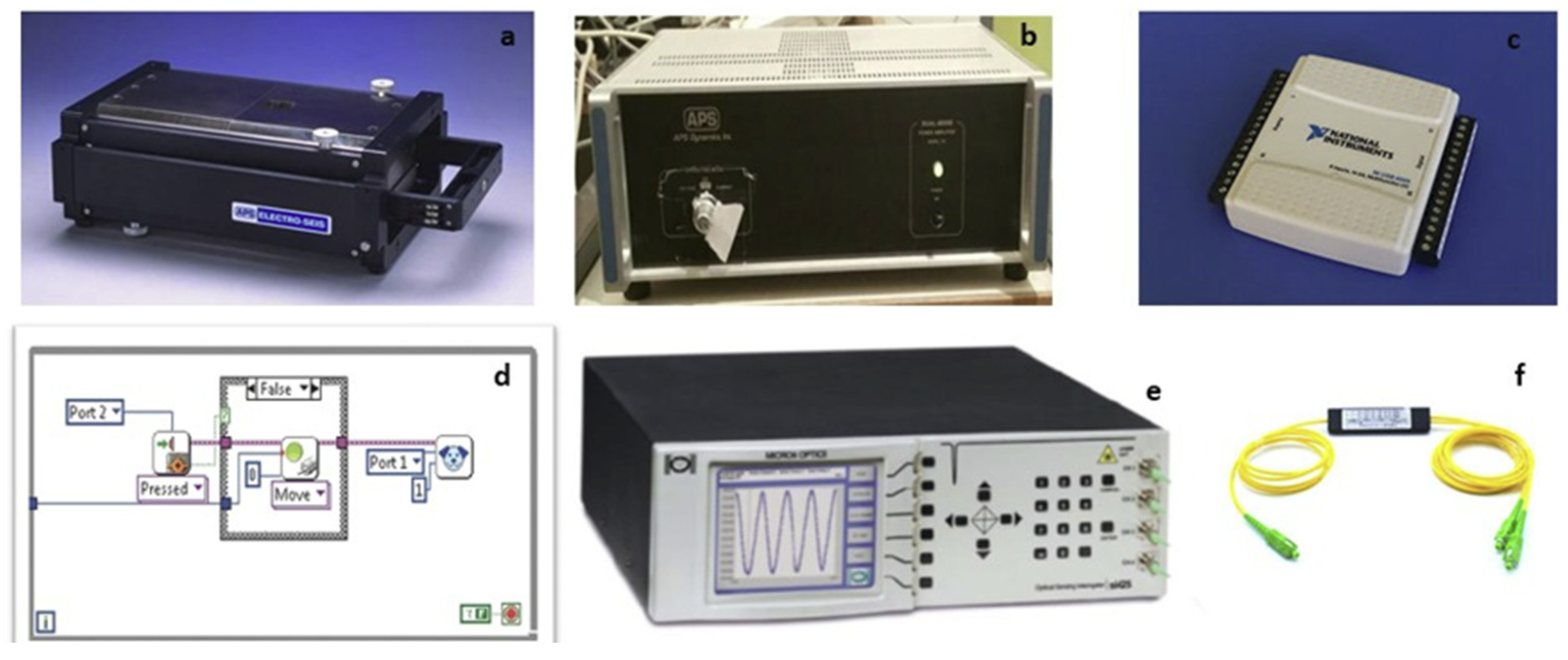
Figure 2.
Unrestrained Sensor, sensor with protective sheathing and sensor attached to a geotextile.
Figure 2.
Unrestrained Sensor, sensor with protective sheathing and sensor attached to a geotextile.
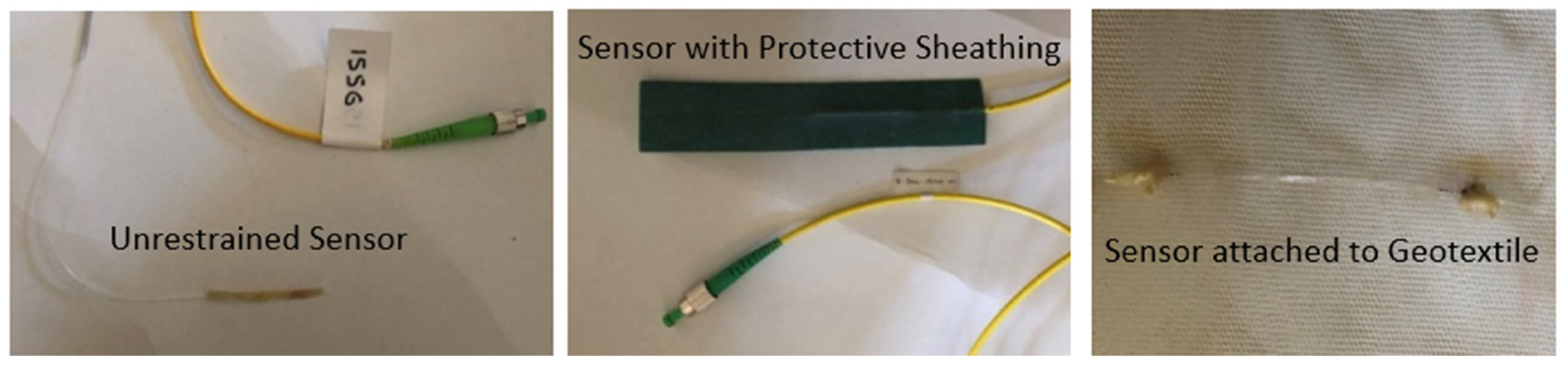
Figure 3.
Sand slope model and geometrical characteristics.
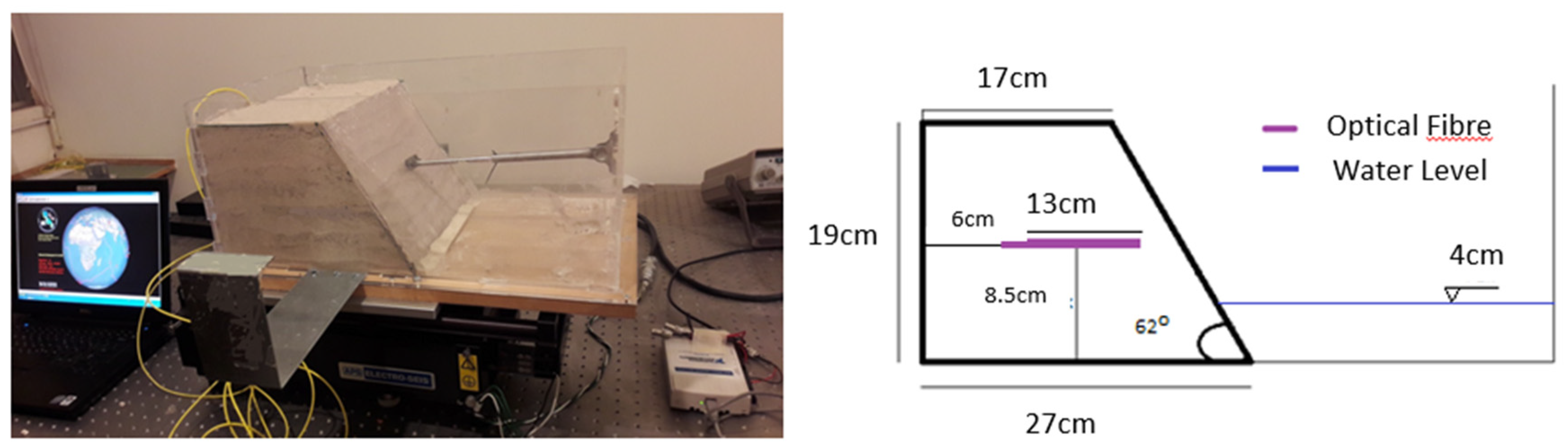
Figure 4.
Slope model behavior under applied loading and resulting failure mechanism.
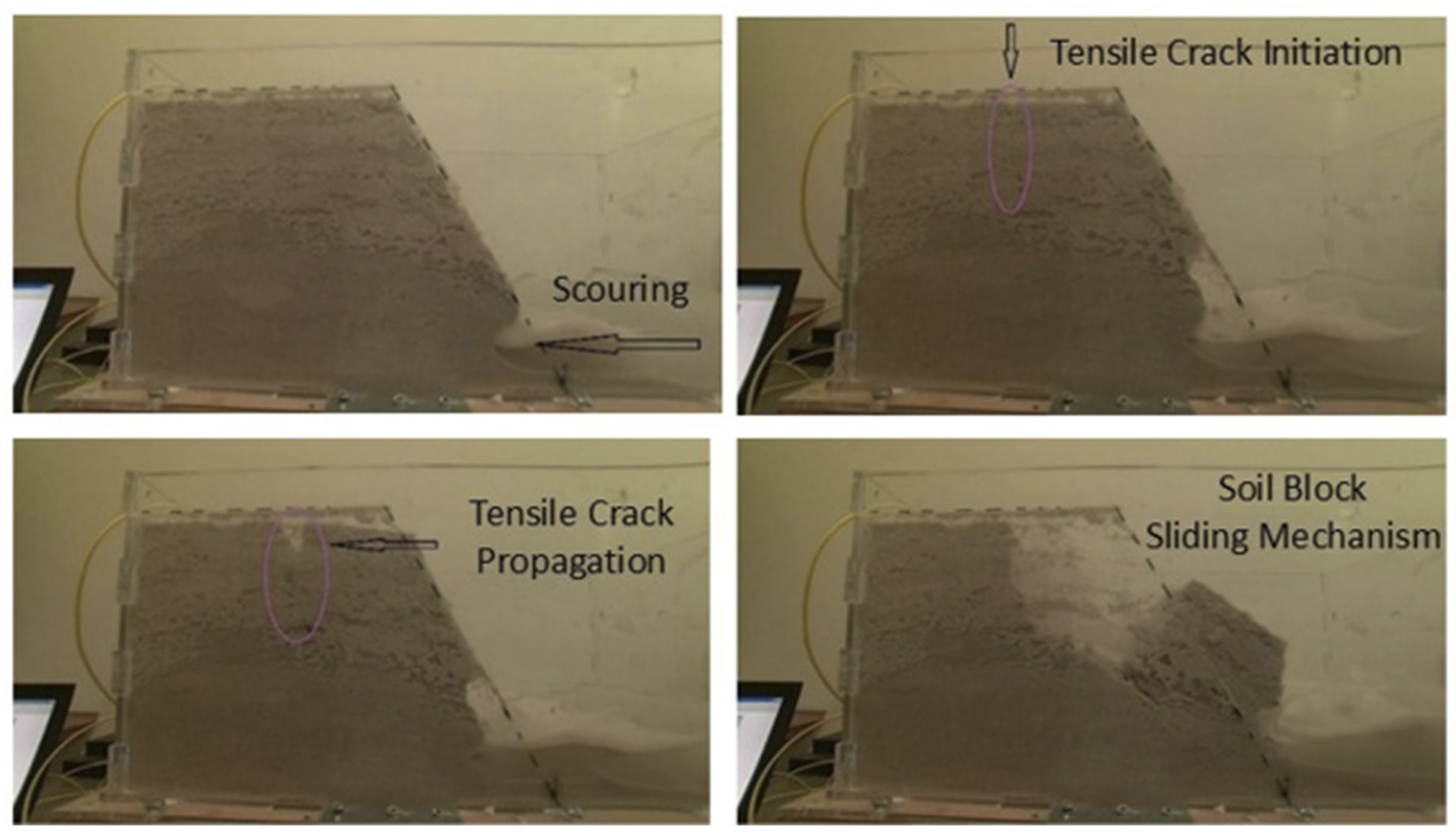
Figure 5.
Strain variation recorded by the optical fiber sensors.
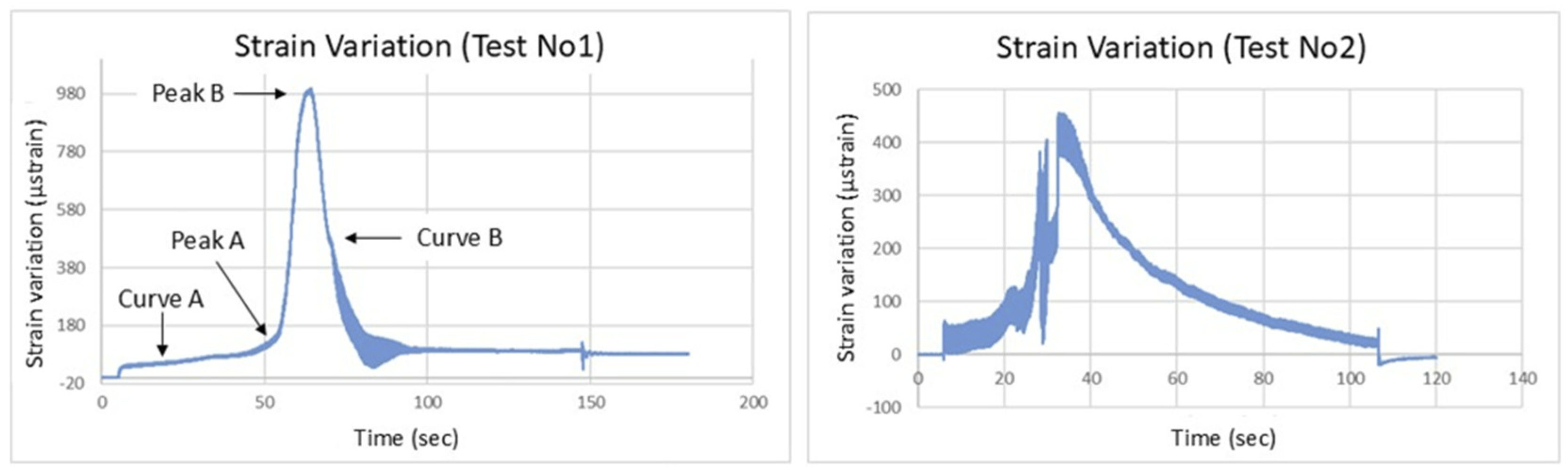
Figure 6.
Analysis using the Bishop Method-SF=0.67 (lef)) and maximum shear strain using the Finite Element method-SRF=0.43 (right).
Figure 6.
Analysis using the Bishop Method-SF=0.67 (lef)) and maximum shear strain using the Finite Element method-SRF=0.43 (right).
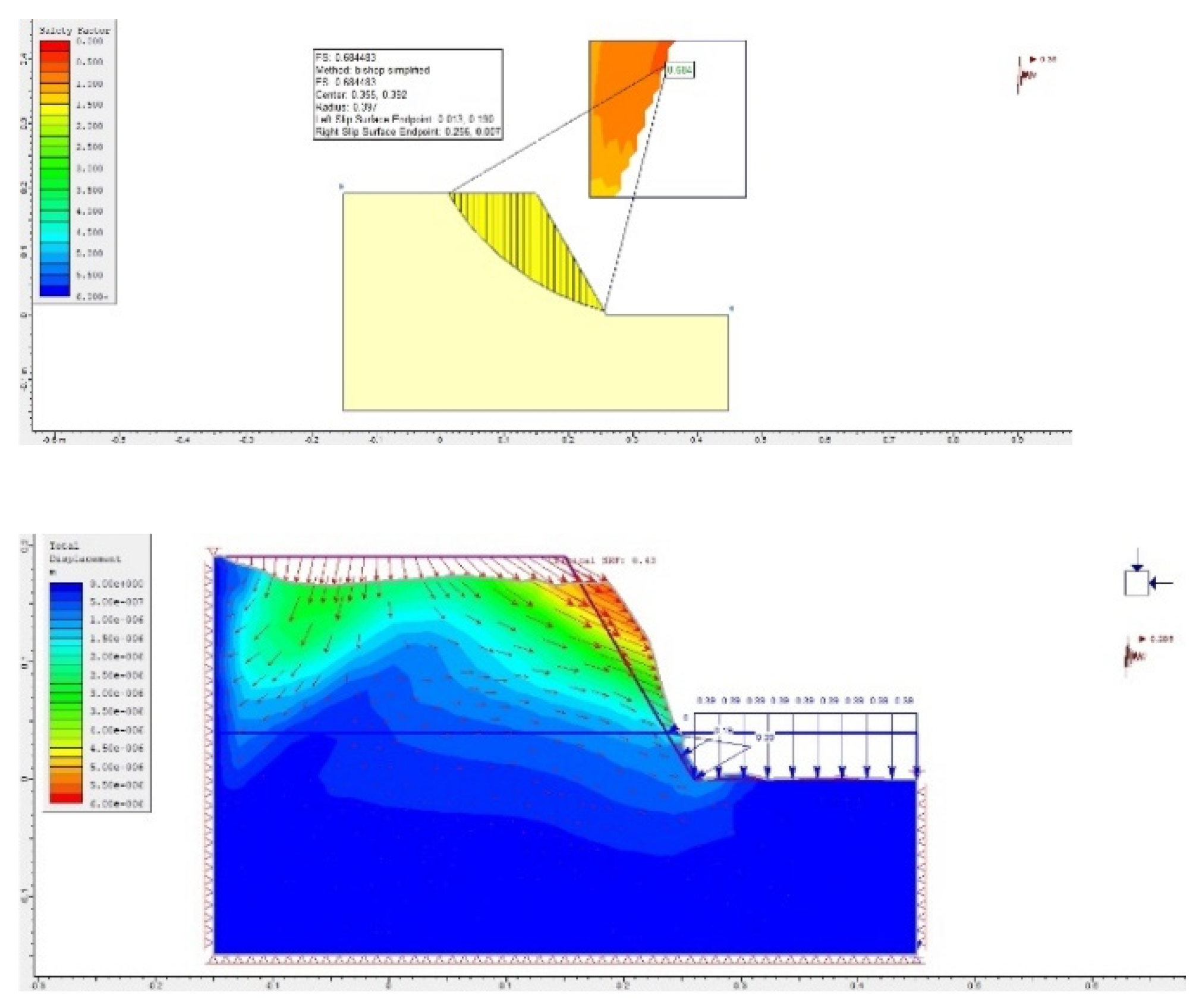
Figure 7.
Side view of the model (left) and the scaled pipe with optical fiber sensor placement (right).
Figure 7.
Side view of the model (left) and the scaled pipe with optical fiber sensor placement (right).
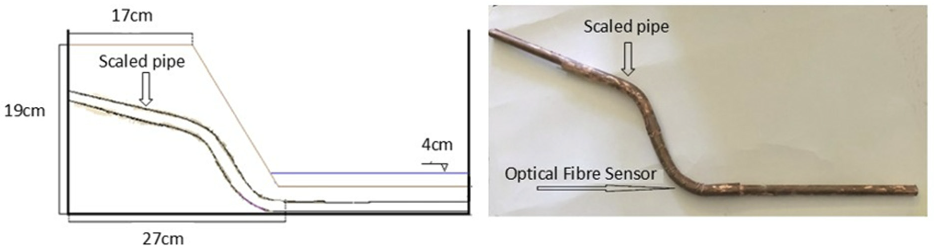
Figure 8.
Model structural response to applied loading, including scour at the slope base and shear initiation at the existing tensile crack.
Figure 8.
Model structural response to applied loading, including scour at the slope base and shear initiation at the existing tensile crack.
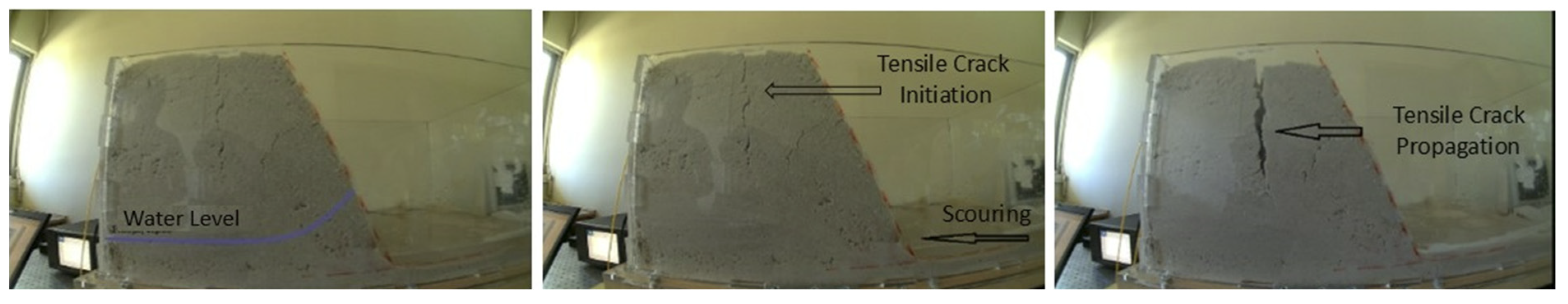
Figure 9.
Strain variation recorded by the optical fiber sensor.
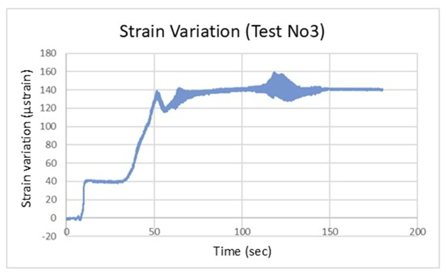
Figure 10.
Reinforced slope model, a side view and failure mechanism.
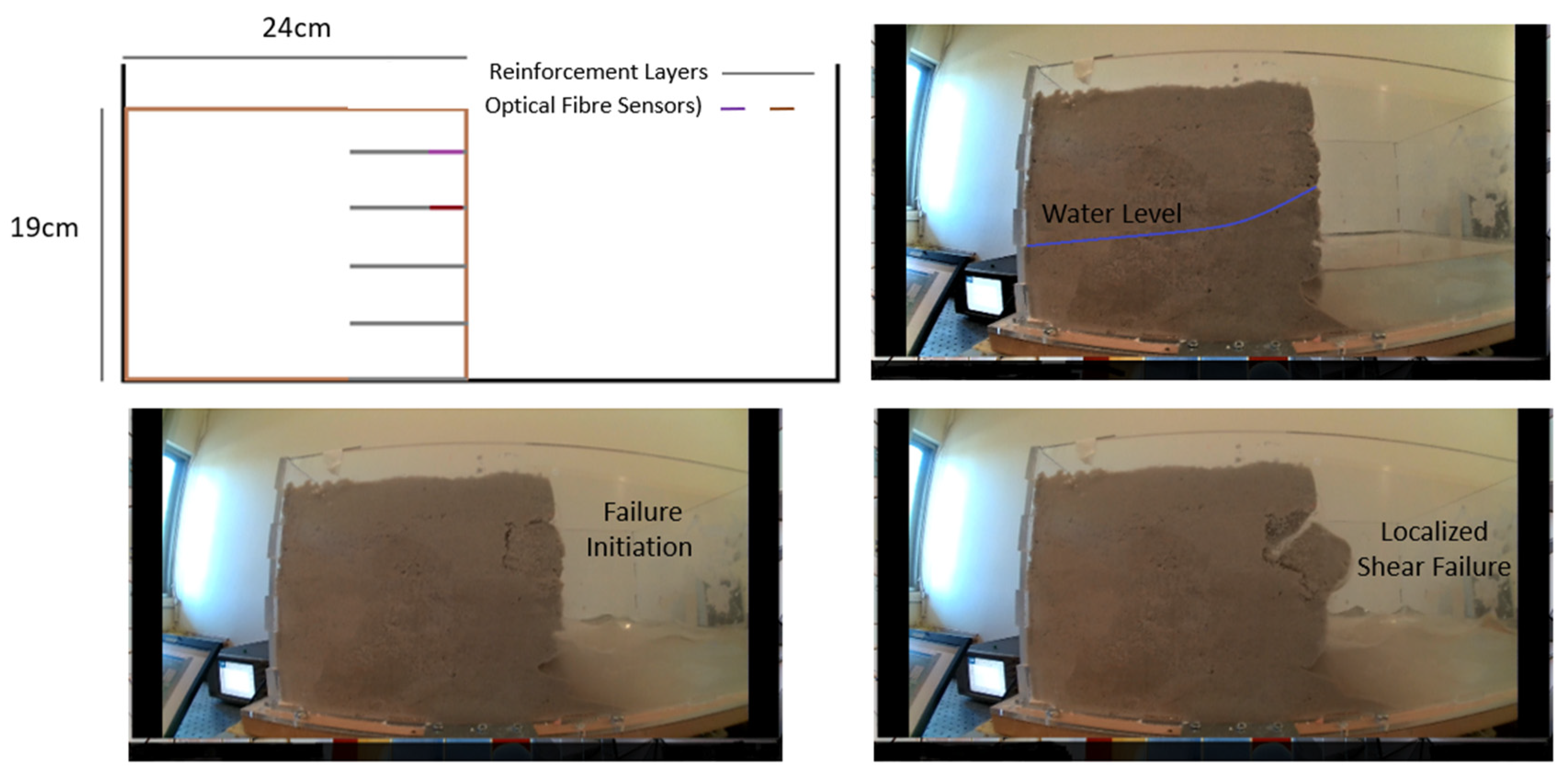
Figure 11.
Strain variation recorded by two optical fiber sensors.
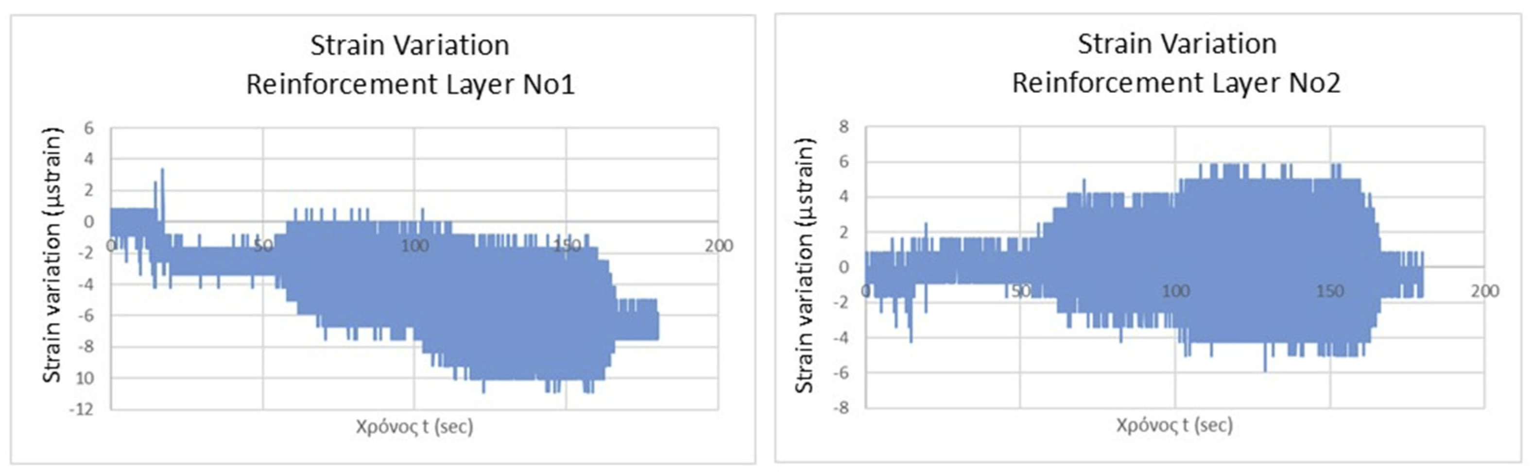
Figure 12.
Scaled reinforced slope model (left), reinforcement layers incorporating optical fiber sensors (middle) and model cross section (right).
Figure 12.
Scaled reinforced slope model (left), reinforcement layers incorporating optical fiber sensors (middle) and model cross section (right).
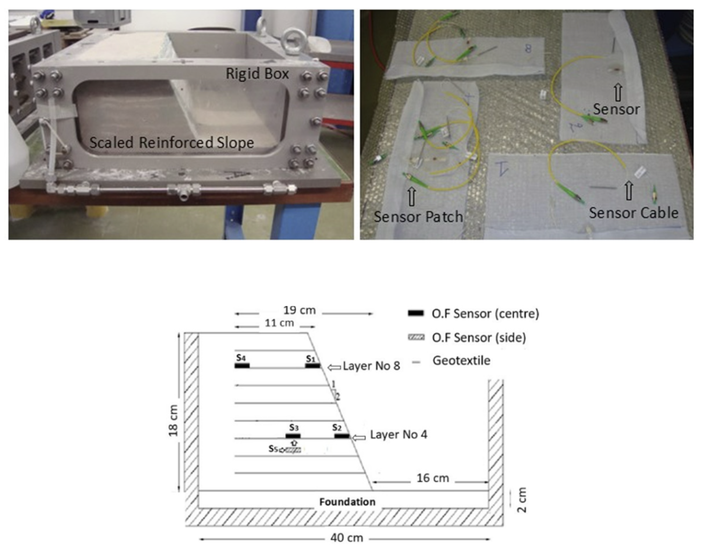
Figure 13.
Test setup (left) and reinforced slope in the centrifuge (right).
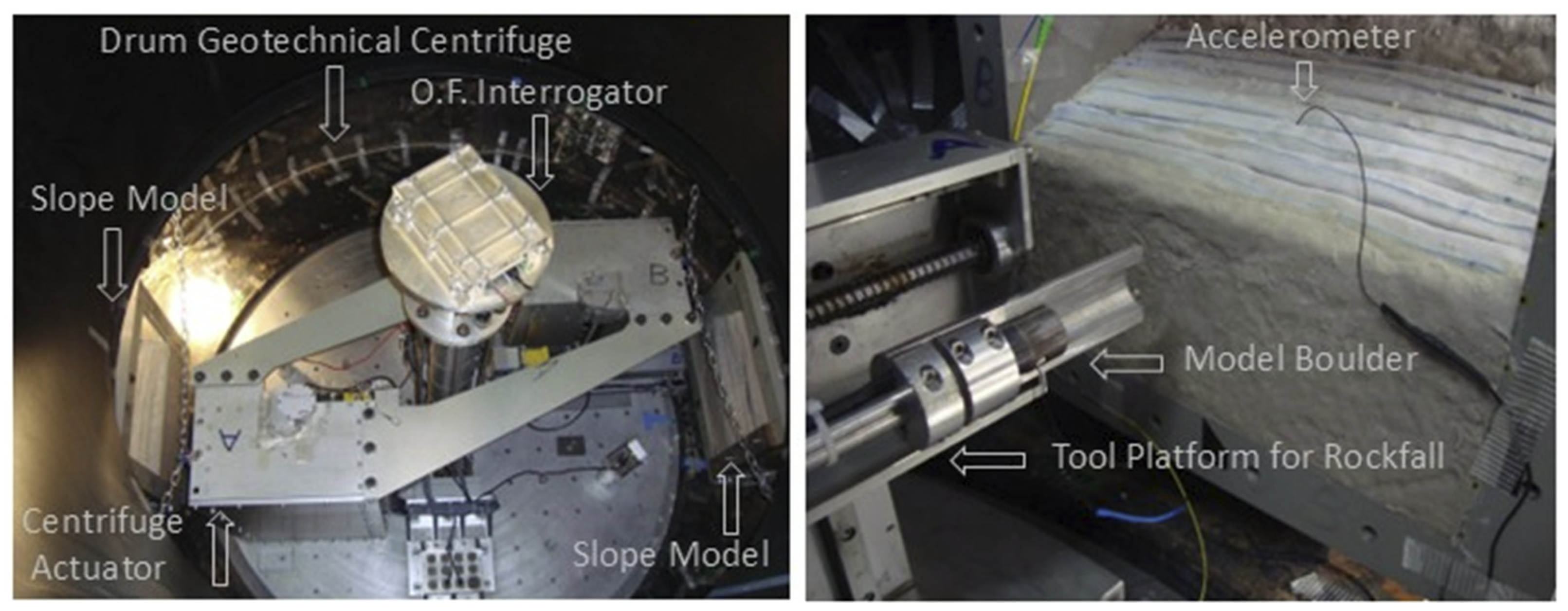
Figure 14.
Strains recodred during Test No.1 (left) and strains recoded during Test No.2 (right).
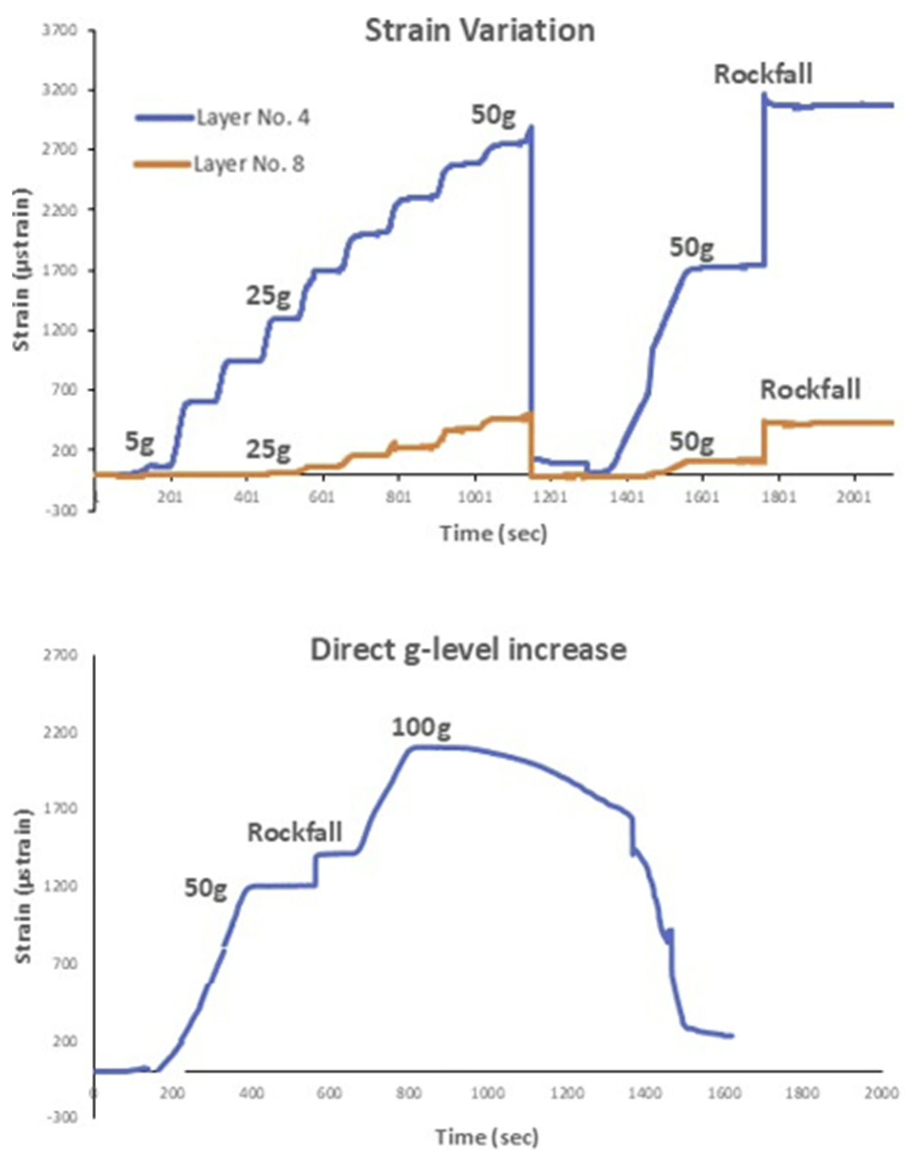
Figure 15.
Flow vectors of soil grains, with vectors colored black representing 1g and vectors colored red indicating 50g (left). Strains calculated via GeoPIV alongside the locations of the optical fiber sensors (right).
Figure 15.
Flow vectors of soil grains, with vectors colored black representing 1g and vectors colored red indicating 50g (left). Strains calculated via GeoPIV alongside the locations of the optical fiber sensors (right).
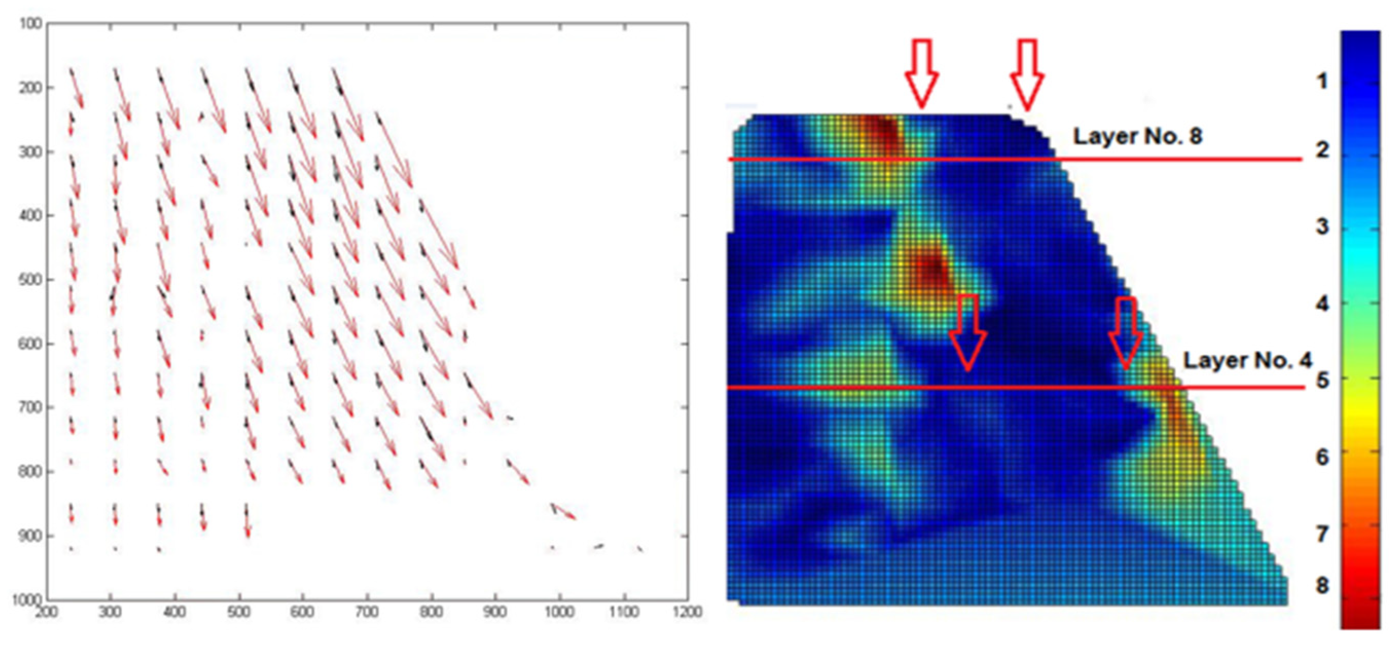
Figure 16.
Cross-section of the southern part of the Circuit Wall (left). A panoramic view of the Acropolis Hill, the Circuit Wall, and the Parthenon from the southeast (right).
Figure 16.
Cross-section of the southern part of the Circuit Wall (left). A panoramic view of the Acropolis Hill, the Circuit Wall, and the Parthenon from the southeast (right).
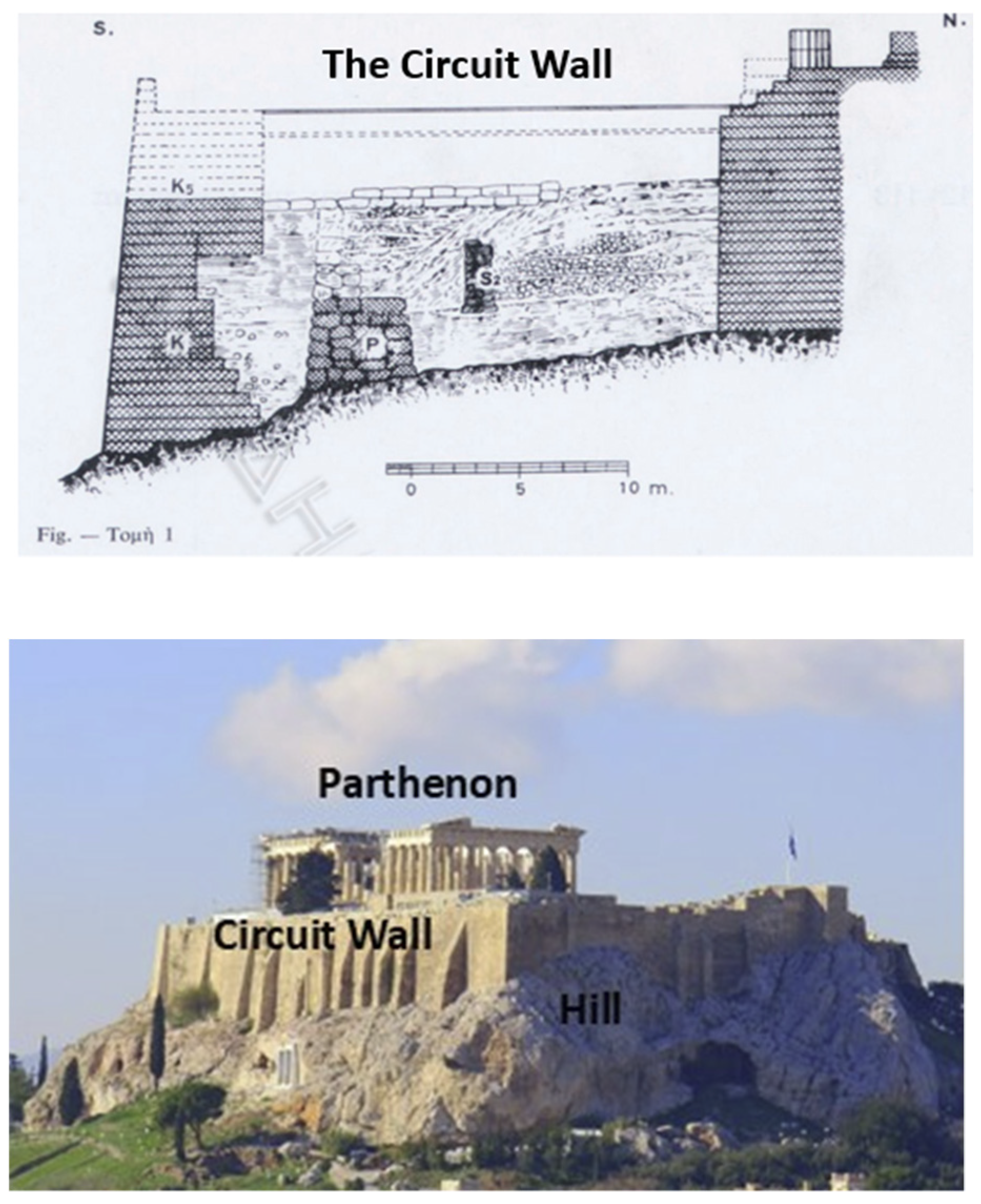
Figure 17.
Locations of the installed optical fiber sensors on the South Wall and Acropolis Hill.
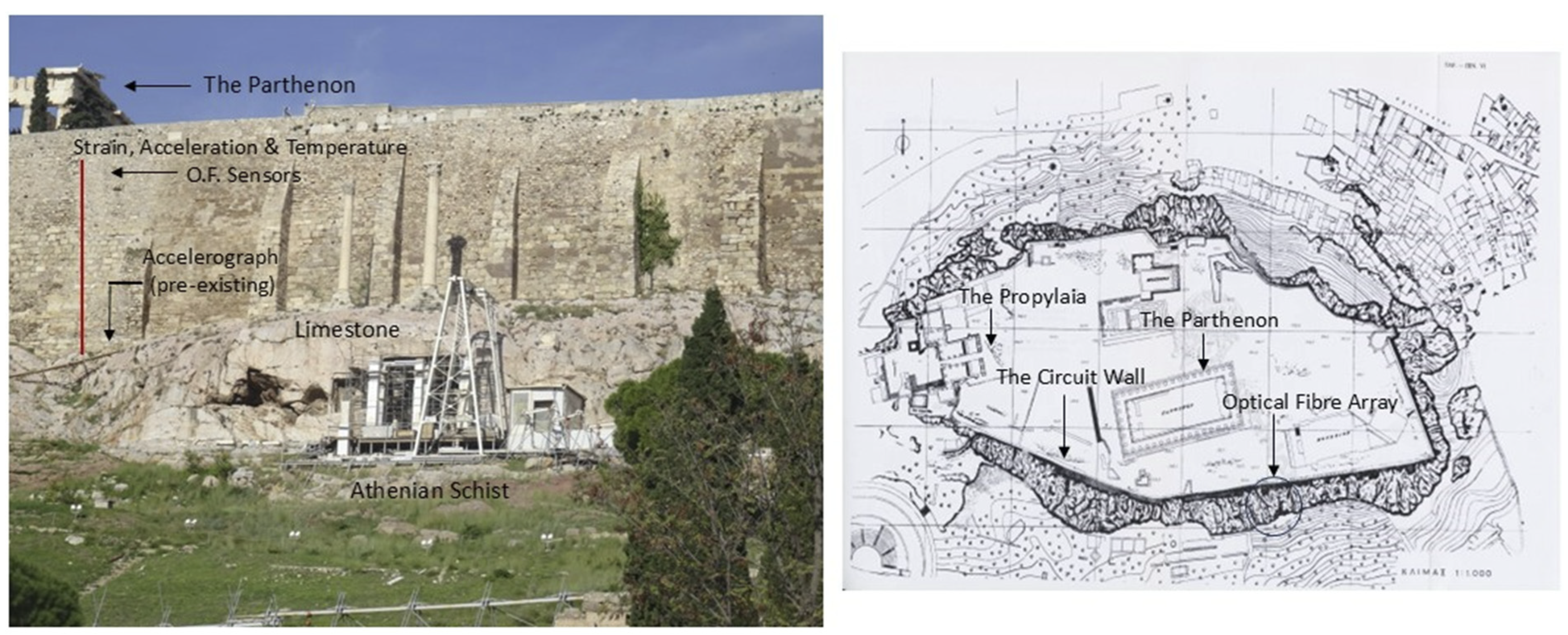
Figure 18.
Strain and temperature FBG sensors on the Wall, including anchoring plates (left) and Acceleration FBG Sensor (right).
Figure 18.
Strain and temperature FBG sensors on the Wall, including anchoring plates (left) and Acceleration FBG Sensor (right).
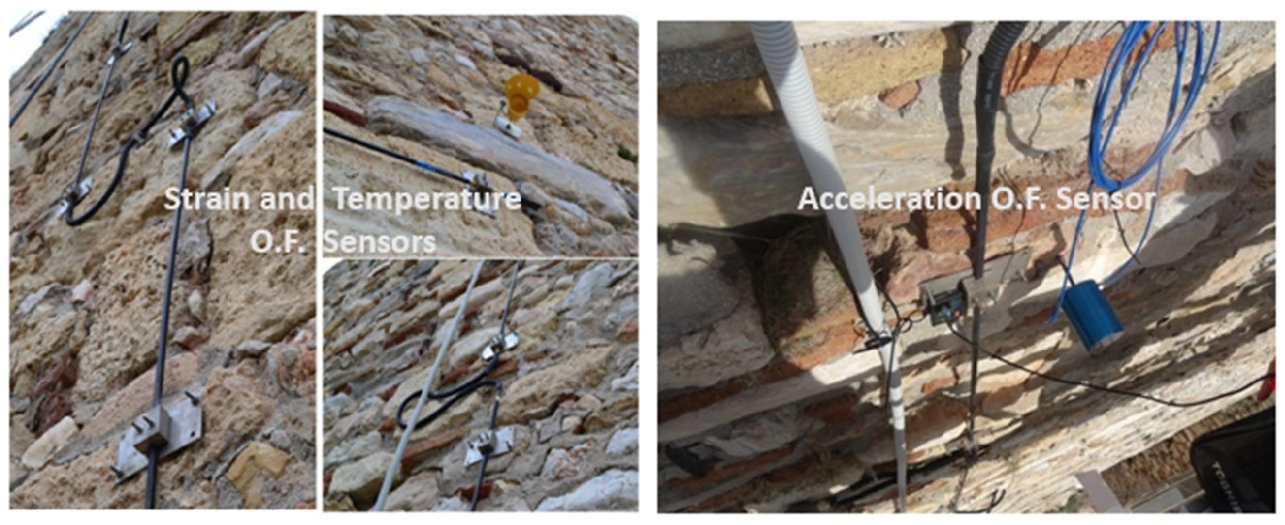
Figure 19.
Configuration of Fiber Bragg Grating sensors, arranged in series and parallel on the South Wall.
Figure 19.
Configuration of Fiber Bragg Grating sensors, arranged in series and parallel on the South Wall.
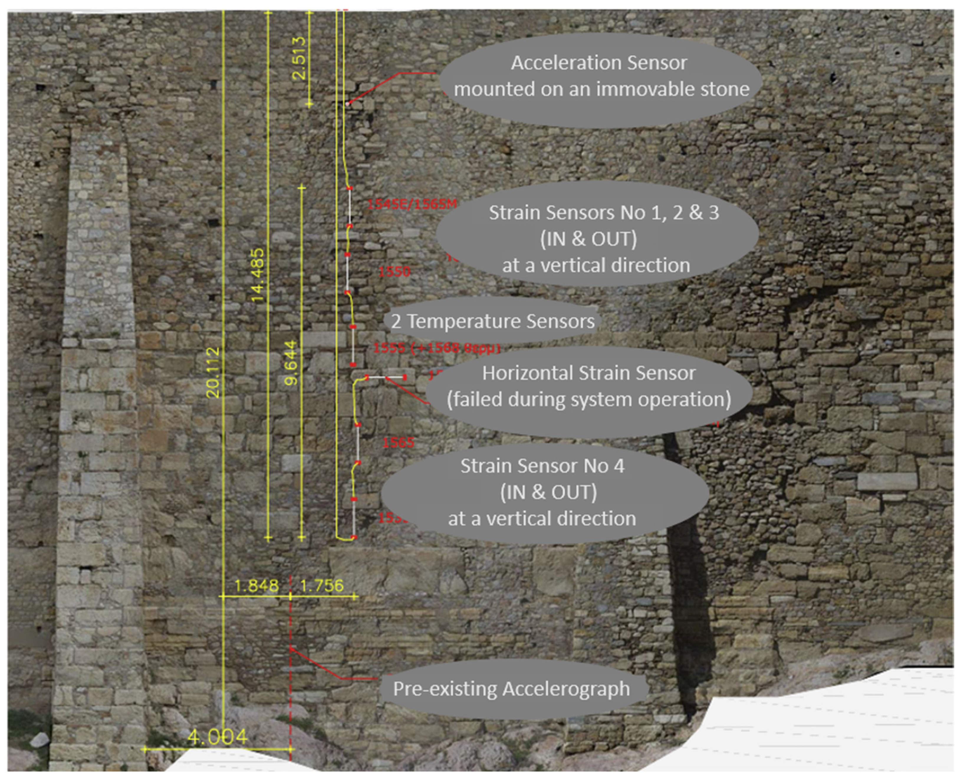
Figure 20.
Comparison of strain variation with and without thermal compensation.
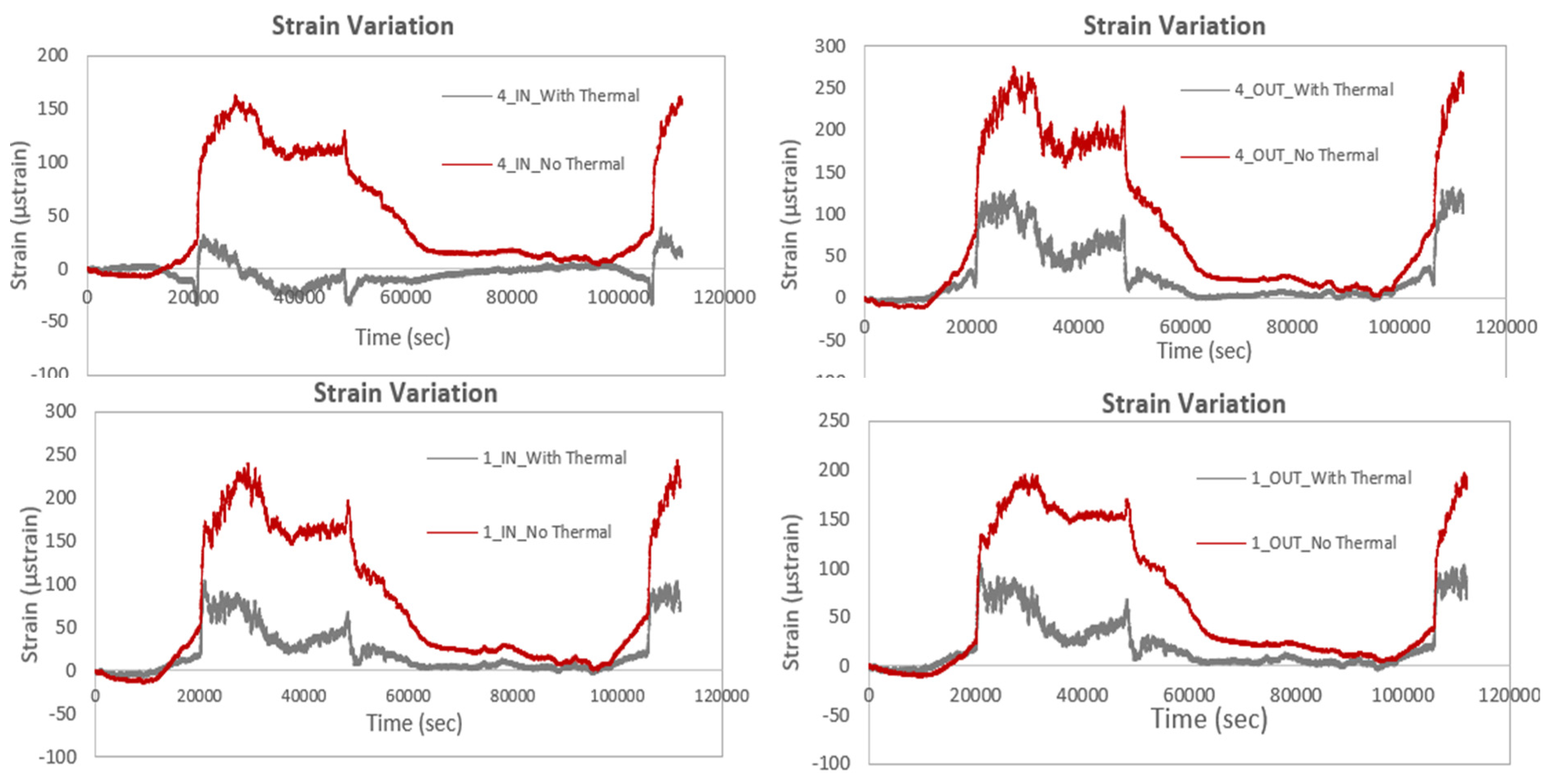
Figure 21.
Comparison of strain variation at the IN and OUT positions for the same smart rods.
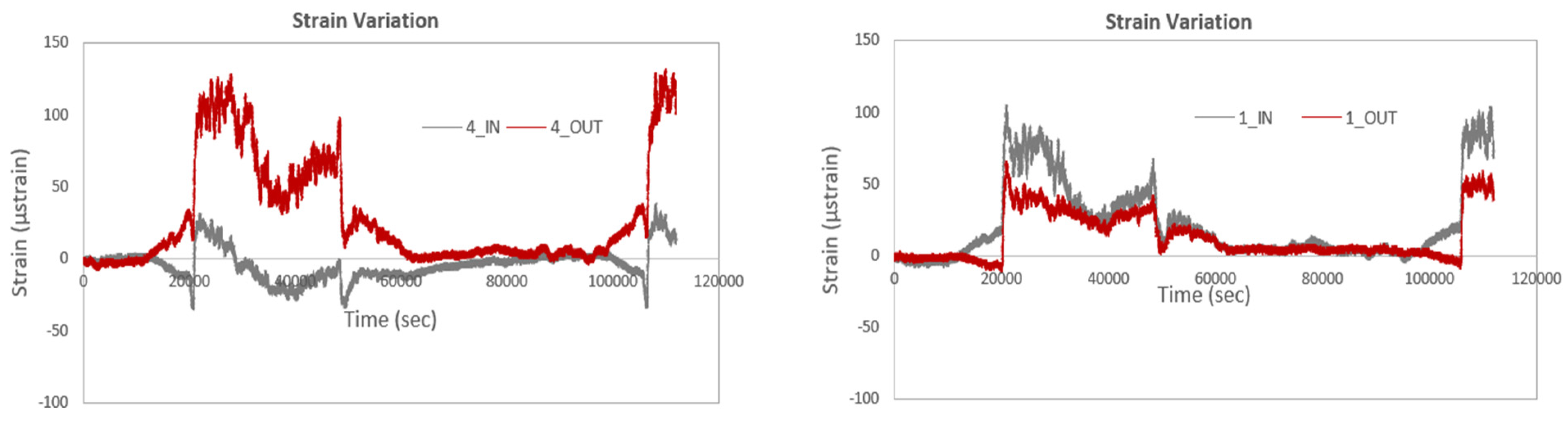
Figure 22.
Strain variation of four sensors at both IN and OUT positions, with thermal compensation.
Figure 22.
Strain variation of four sensors at both IN and OUT positions, with thermal compensation.
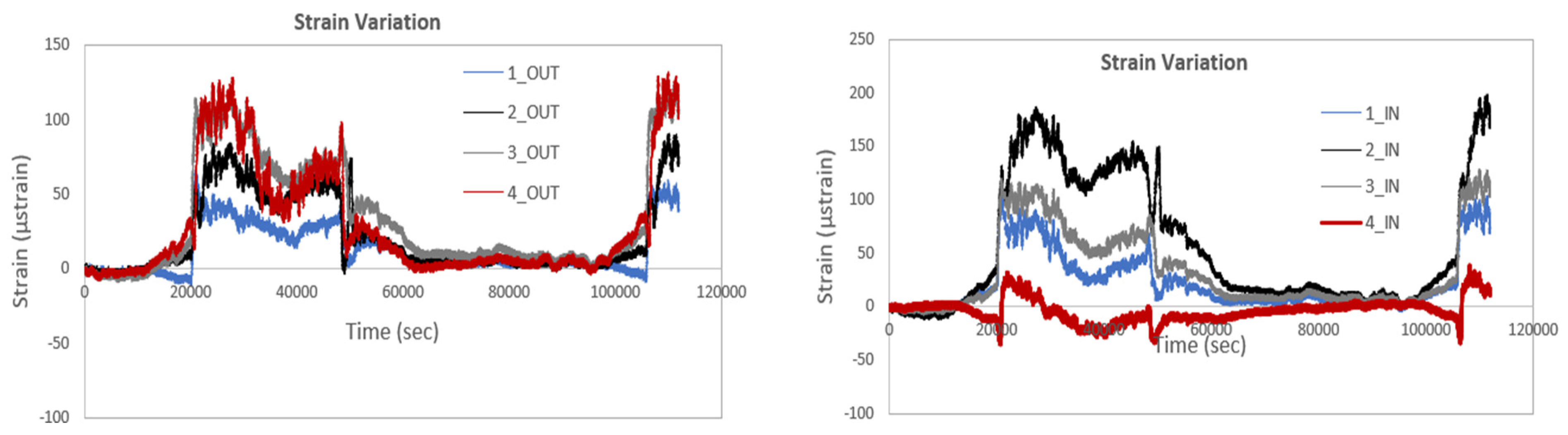
Figure 23.
Acceleration levels recorded by the single-axis acceleration sensor with and without thermal compensation (left) and temperature variation (right).
Figure 23.
Acceleration levels recorded by the single-axis acceleration sensor with and without thermal compensation (left) and temperature variation (right).
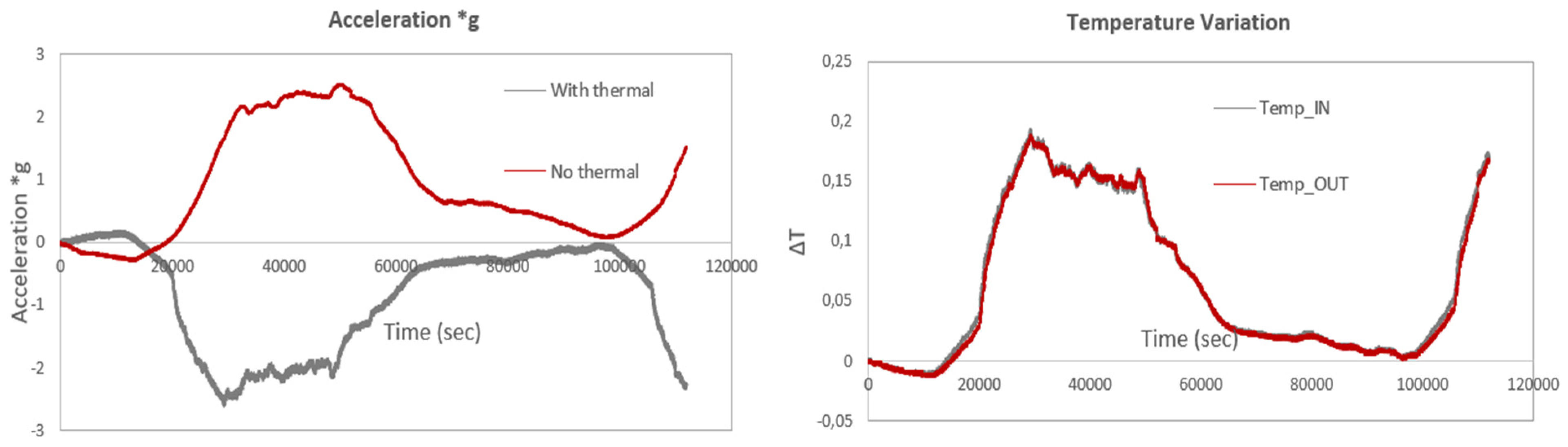
Figure 24.
Acceleration levels recorded by the single-axis acceleration sensor with and without thermal compensation (left) and temperature variation (right).
Figure 24.
Acceleration levels recorded by the single-axis acceleration sensor with and without thermal compensation (left) and temperature variation (right).
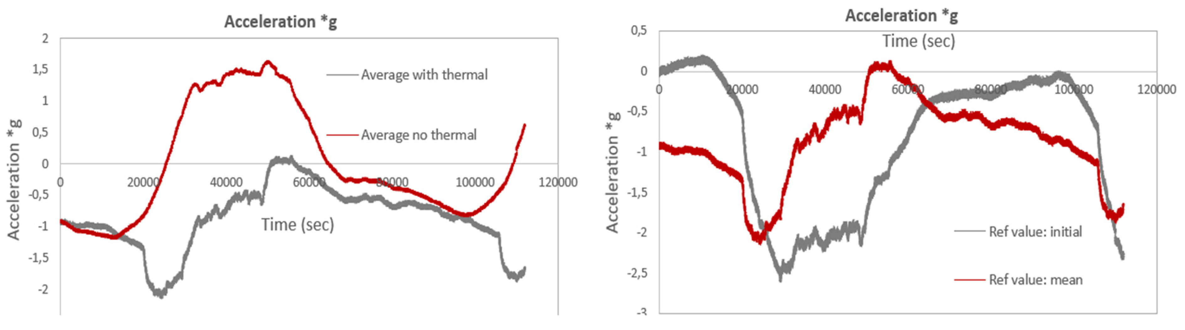

Table 1.
Single-axis acceleration sensor specifications.
| Specifications | |
| Sensitivity | 75 pm/g @ 40 Hz |
| Measurement range | ± 10 g |
| Frequency range | 0 to 50 Hz |
| Resonance frequency | 430 Hz |
| Flatness | < 2% |
| Resolution | 12.5 μg/√Hz |
| Maximum calib. Error | ±0.1 g @ 40 Hz |
| Transverse sensitivity | < 0.1% |
Disclaimer/Publisher’s Note: The statements, opinions and data contained in all publications are solely those of the individual author(s) and contributor(s) and not of MDPI and/or the editor(s). MDPI and/or the editor(s) disclaim responsibility for any injury to people or property resulting from any ideas, methods, instructions or products referred to in the content. |
© 2025 by the authors. Licensee MDPI, Basel, Switzerland. This article is an open access article distributed under the terms and conditions of the Creative Commons Attribution (CC BY) license (http://creativecommons.org/licenses/by/4.0/).
Copyright: This open access article is published under a Creative Commons CC BY 4.0 license, which permit the free download, distribution, and reuse, provided that the author and preprint are cited in any reuse.


