
Submitted:
01 January 2025
Posted:
02 January 2025
You are already at the latest version
Abstract
In modern audio processing systems like speech recognition, medical devices, and IoT sensors, effective noise filtering is crucial. High noise levels degrade signal quality and reduce system accuracy. Traditional methods often fail under high noise, requiring new approaches. This paper presents an innovative method combining horizontal visibility graph (HVG) features with the LogNNet neural network, previously unused for audio noise filtering. LogNNet operates in regression mode, predicting the original signal from features extracted from the noisy input. This approach allows the model to reconstruct clean signals by analyzing patterns within the noisy data, improving filtering accuracy. Experiments show that HVG features in LogNNet significantly reduce MAE in noisy audio, achieving up to 70% noise reduction for high noise levels (Noise = 0.3–0.4). As the number of features increases (NF = 21), the impact of HVG lessens, indicating parameter saturation. Cascading LogNNet models progressively reduce noise until further filtering becomes ineffective. This method shows strong potential for real-world audio tasks, including speech recognition and IoT. The paper highlights HVG’s importance in enhancing LogNNet’s noise robustness. Future research will focus on expanding model architecture and training on diverse noise types to improve accuracy and reliability.
Keywords:
Signal Denoising
; LogNNet Neural Network
; Horizontal Visibility Graph (HVG)
; Audio Signal Processing
; Noise Reduction
; Time Series Analysis
; Machine Learning
; Feature Extraction
; Cascade Filtering
; Speech Enhancement
1. Introduction
Noise filtering is a key stage in audio signal processing that improves the signal-to-noise ratio, enhances speech and audio quality, and increases the accuracy of recognition algorithms. Noise varies in nature and spectral characteristics, imposing different requirements on filtering and signal processing methods. Modern communication and audio processing systems actively employ various noise suppression techniques to ensure data transmission stability and minimize distortion [1].
Current noise filtering methods fall into two main categories:
- Traditional methods – spectral filtering, wavelet transforms, and adaptive filters (such as the Kalman filter). These approaches yield stable results under low-noise conditions.
- Machine learning methods – deep neural networks (DNNs), convolutional neural networks (CNNs), recurrent neural networks (RNNs), and transformers, which adapt to noise characteristics and effectively filter complex noise profiles. The primary idea behind filtering in these methods is to represent the signal as a mel-spectrogram and feed it into a CNN.
However, the approach proposed in this paper is novel and based on regression algorithms that predict the amplitude of the audio signal. Unlike traditional approaches, this method relies on the LogNNet neural network and unique features extracted from horizontal visibility graphs (HVG). This approach enables efficient prediction of the dynamics of noisy audio signals, enhancing filtering accuracy and making the system more resilient to various types of interference.
1.1. Main Types of Noise
The primary types of noise include:
- White Noise – Noise with uniform spectral density across the entire frequency range. It appears as synthetic noise generated by software (e.g., in Python, this type of noise can be simulated using the function np.random.uniform from the NumPy library) and is often used to simulate background noise in experiments [2]. White noise serves as the basis for modeling many other types of noise.
- Gaussian Noise – A type of white noise where the amplitudes follow a normal distribution. This is the most common model of random interference in audio signals and radio systems. In Python, it can be generated using the function np.random.normal.
- Babble Noise [3] – The cumulative effect of overlapping voices, often used to simulate background noise in public spaces.
- Industrial Noise [4] – Noise generated by machines and mechanisms, frequently encountered in industrial environments. It is characterized by broadband and random distribution.
- Diffuse Noise [5] – Noise that arises in reverberant environments when the noise source is surrounded by reflective surfaces. This type of noise is difficult to filter due to its stochastic nature.
- Pink Noise [6](1/f Noise, Flicker Noise) – Noise with an intensity inversely proportional to frequency. Pink noise is commonly found in real-world systems and audio recordings.
- Impulse Noise [7] – Short, powerful pulses that often occur during electronic device switching or as interference in electrical systems.
White noise is one of the most challenging types of noise to filter. In the study by Hermus et al. [8], a review of speech enhancement methods under additive stationary noise, including white Gaussian noise, is presented. The authors emphasize that white noise poses a significant obstacle for speech recognition systems, necessitating the development of more robust algorithms. Grumiaux et al. [9] explore sound source localization methods based on deep learning and note that white Gaussian noise significantly reduces the accuracy of source localization. The authors highlight the need for resilient algorithms to mitigate this type of noise. In the work by Salvati et al. [10], neural networks are described as effective tools for improving sound localization in noisy and reverberant environments. The authors indicate that white Gaussian noise is added to each channel to simulate complex conditions.
1.2. Principles of Audio Signal Noise Filtering Using Neural Networks
Convolutional neural networks are widely used for audio signal analysis due to their ability to extract key features from spectrograms [11]. Special attention is given to Mel-spectrograms [12,13,14], which transform audio signals into two-dimensional representations. The X-axis represents time, while the Y-axis represents frequency on a logarithmic Mel scale. Mel-spectrograms are fed into convolutional networks, making audio processing tasks resemble image processing.
Principle of Convolutional Neural Network (CNN) Operation with Audio:
Step 1: Signal Transformation
The audio signal (e.g., WAV or MP3) is converted into a Mel-spectrogram.
Step 2: Normalization
The data is amplitude-normalized to reduce differences in volume.
Step 3: Noise Suppression
Two-dimensional filters are applied in convolutional layers to detect and suppress noise patterns. The CNN learns to differentiate between noise and useful signals by recognizing key features.
Step 4: Post-Processing
The clean audio signal is reconstructed by applying an inverse spectrogram transformation back into audio (e.g., using the Griffin-Lim algorithm).
The combination of CNNs and Mel-spectrograms demonstrates high efficiency in audio noise filtering. The core principle involves transforming audio into a spectrogram and using convolutional filters trained to separate noise from useful signals.
A similar approach is applied to images. Singh et al. [15] show that CNNs used in active noise control (ANC) effectively filter out Gaussian additive white noise from computed tomography (CT) images while preserving fine details. Their proposed method integrates noise modeling with a deep learning-based CNN framework. In this process, noisy CT images are generated by adding Gaussian noise at varying levels (σ = 10, 15, 20, 25). The CNN iteratively denoises the images by distinguishing between the underlying structure and noise, improving image quality and preserving essential details.
1.3. Horizontal Visibility Graphs and Noise Suppression
Time series analysis plays a crucial role in various scientific fields, including physics, biology, finance, and engineering. One innovative method for analyzing time series data is the transformation of time series into complex networks through visibility graph algorithms. Visibility graphs provide a powerful framework for uncovering hidden structures, detecting periodicities, and characterizing the complexity of time series data [16]. This review explores the fundamentals of visibility graph techniques, their applications in noise filtering, and their significance in detecting and characterizing signals. Luque et al. [17] present horizontal visibility graphs (HVGs) as a tool designed to distinguish random time series from chaotic ones.
HVGs were used to analyze time series and demonstrated effectiveness in detecting random noise. The method differentiates random processes by the exponential distribution of node degrees, a characteristic unique to uncorrelated random series. This exponential distribution reflects the lack of long-term correlations and periodicities in random data. Furthermore, the study highlighted that for periodic and fractal series, the degree distribution deviates from this exponential form, enabling HVGs to identify and classify different types of signals. This makes HVGs particularly useful for noise filtering, structure detection, and distinguishing stochastic processes from deterministic chaotic dynamics. The research conducted by Núñez et al. [18] delves into the use of HVGs for unveiling hidden periodicities within noisy time series. Their work introduces a graph-theoretical noise filter that effectively isolates periodic elements from background noise. This innovative approach has proven to be highly beneficial in the analysis of biological time series, where distinguishing essential signals from random fluctuations is vital for accurate interpretation. Lacasa et al. [19] applies HVGs to analyze the irreversibility of time series. A method was proposed to assess the degree of irreversibility using visibility graphs, which helps detect nonlinear processes and noise distortions. This approach proved effective for identifying chaos and noise reduction. In [20] application of weighted horizontal visibility graphs (WHVGs) for fault diagnosis of bearings through vibration signal analysis is presented.
HVGs isolates impulse components from noisy signals, making the method valuable for industrial equipment monitoring. Graph Fourier transform (GFT) combined with HVGs improved noise resistance and fault detection accuracy. A method for detecting temporal communities in biological time series based on HVG was introduced by Zheng et al. [21]. This approach identified key biological signals while filtering noise. The method was effective in analyzing unevenly distributed time data, making it valuable for complex biosignal analysis. The study by Iacovacci and Lacasa [22] investigated the capability of HVG to distinguish between noise and useful signals. The authors applied a method that transforms time series into graphs, where nodes represent points in the time series, and edges connect nodes that satisfy the horizontal visibility condition. The focus was placed on analyzing the graph’s structure, including changes in topology depending on the signal’s nature, such as node degree, cluster distribution, and other network characteristics. HVG was employed to filter out random noise, enabling the separation of noise from the systematic components of the signal. Topological features identified through HVG demonstrated high efficiency in isolating noise. The results of the study confirmed the method’s potential in noise suppression tasks due to its high accuracy and reliability.
Thus, horizontal visibility graphs (HVG) are successfully applied to noise filtering, fault diagnosis, biological and industrial time series analysis, and neurobiology. This method is distinguished by its accuracy and resilience to noise distortions, making it a valuable tool for time series analysis.
Despite the broad applicability of HVG, the use of node degrees as direct features for neural network input in noise suppression tasks remains unexplored. To date, node degree sequences have primarily been leveraged in entropy-based approaches for time series classification, as demonstrated in our previous work (Conejero et al. [23]). In that study, the degree sequences of HVG were utilized to compute entropy, facilitating the classification of time series by their functional characteristics. However, the potential of directly feeding node degrees into neural networks for noise filtering presents an intriguing and largely untapped direction for future research.
1.4. LogNNet Neural Network
LogNNet is a neural network model that utilizes logistic maps or linear congruential generators to populate the reservoir matrix. This approach enhances computational efficiency, making LogNNet particularly suitable for low-memory environments, such as IoT devices and embedded systems. The model was proposed by Velichko [24], and since its inception, it has been applied in various fields, including medical diagnostics [25,26], time series analysis [27], and image classification [28].
Key applications of LogNNet span across medical diagnostics, IoT systems, and low-resource environments, demonstrating its versatility and computational efficiency. In the study by Huyut and Velichko [29], LogNNet was applied for the diagnosis and prognosis of COVID-19, leveraging logistic mapping to analyze medical data, providing a fast and economical AI tool for clinical use. Velichko [30] introduced LogNNet as a method for medical data analysis, emphasizing its utility in clinical decision support systems and edge computing in healthcare by utilizing linear congruential generators to enhance performance. Further applications in COVID-19 diagnostics were explored by Huyut and Velichko [31], where routine blood data was processed using LogNNet’s chaotic reservoir matrix to improve diagnostic accuracy. The model was also employed in detecting right ventricular dysfunction, as described by Huyut et al. [32], using pulmonary embolism datasets with reservoir matrices populated bylogistic map outputs. In the domain of IoT and low-resource environments, Izotov et al. [33] applied LogNNet to recognize handwritten MNIST digits on Arduino boards with only 2 Kb of RAM, emphasizing the lightweight architecture of the model. LogNNet’s adaptability was further demonstrated in emotion recognition tasks by Velichko and Izotov [34], using keystroke dynamics datasets, highlighting its versatility beyond traditional image and medical data analysis. Additionally, Velichko et al. [35] explored broader IoT applications, showcasing LogNNet’s potential in smart environments and IoT-enabled intelligent systems.
With the release of version 1.7, LogNNet has been refined to feature low resource consumption, high processing speed, and the capability to perform regression tasks. These enhancements make LogNNet an ideal choice for noise reduction applications, particularly those involving time series prediction.
1.5. Major Contributions
In this paper, we introduce an innovative method for noise suppression in audio signals by integrating HVG features with the LogNNet neural network. This approach addresses the limitations of traditional noise filtering techniques, which often struggle with high noise levels. We demonstrate that the use of HVG-derived features significantly reduces mean absolute error (MAE) during the processing of noisy audio signals, achieving up to 70% noise reduction, particularly for high-noise environments (Noise = 0.3-0.4).
The major contributions of this paper are the following ones:
- A novel methodology combining HVG features with the LogNNet neural network is proposed for audio signal noise suppression. This marks the first application of LogNNet for audio denoising, showcasing its potential for improving signal quality in speech recognition systems and IoT devices.
- The effectiveness of HVG features in enhancing noise suppression is validated experimentally. For models with low feature counts (HW = 1), the addition of HVG features leads to substantial improvements in filtering performance. However, as the feature count increases (HW = 10), the influence of HVG features diminishes, indicating a saturation point where the model is sufficiently parameterized.
- A cascading model application technique is introduced, demonstrating that iterative noise reduction using multiple LogNNet models can progressively lower noise levels. This cascading approach is shown to improve filtering performance until a threshold is reached, beyond which further iterations degrade signal quality.
- The paper highlights the development of datasets and testing protocols, including audio files generated with varying levels of Gaussian white noise, to rigorously evaluate the proposed method. Metrics such as R² and mean absolute error (MAE) are used to quantify performance improvements across different noise levels.
This work opens new avenues for adaptive noise suppression in audio processing applications, with potential implications for speech enhancement, medical devices, and IoT sensor systems [36,37]. Future research will focus on expanding the model architecture and training it on diverse noise types to enhance robustness and accuracy across various real-world scenarios.
2. Methods
2.1. Training and Testing Audio Files
The gTTS (Google Text-to-Speech) library in Python was used to generate audio files, enabling the conversion of text into speech [38]. The conversion process involved multiple stages, resulting in audio signals saved in WAV format and represented as time series.
The training phrase used was:
“Hello, world! Let’s create together!”
- Sampling rate: 24,000 Hz
- Channels: 1
- Duration: 3.432 seconds
- Number of discrete time series elements: 82,368
For testing, the following phrase was used:
“Zero excuses, One goal, Two steps forward, Three ideas in motion, Four milestones achieved, Five dreams alive!”
- Sampling rate: 24,000 Hz
- Channels: 1
- Duration: 11.736 seconds
- Number of discrete time series elements: 281,664
To train LogNNet for noise filtering, audio signals were simulated by adding white (Gaussian) noise with a normal distribution. The noise level was set at six values: 0.01, 0.05, 0.1, 0.2, 0.3, and 0.4, where each value corresponds to a fraction of the maximum amplitude of the original signal. Noise was added using the np.random.normal function from the NumPy library, which generates arrays of normally distributed random numbers. Figure 1 illustrates the time series of the original training audio signal and the noisy signals at various levels of noise components. It is evident that at Noise = 0.4, the audio patterns become nearly indistinguishable; when played back, it is difficult to recognize the spoken information. All original and noisy audio files in .wav and .csv formats are provided in the appendix.
2.2. Training and Testing Datasets for LogNNet
As part of this work, datasets were created to train the LogNNet neural network. The dataset is represented by a CSV file with named columns containing data derived from two audio signals — the original audio file and the noisy audio file. The primary goal of this procedure was to extract features and target values that can be used to train machine learning models aimed at effectively filtering signals from noise.
The output data formation involved the following steps:
- The half-window size HW was determined (Figure 2), specifying the number of time steps from the center to the edge of the window, used to form the features. Features were extracted from the area surrounding the current target signal value.
- For each point in the time series within the range from HW to (audio file length - HW), the target value was extracted from the original (clean) signal. Corresponding features included the values of the noisy signal on both sides of the current point.
During the experiment, five training and five testing datasets were generated based on audio files with different noise levels (Noise = 0.01, 0.05, 0.1, 0.2, 0.3, 0.4). The clean (non-noisy) signal was used as the target column, while features were extracted from the noisy time series.
Feature extraction was performed using a window centered around the target element t, with indices ranging from t−HW to t+HW. The values of half-window size HW were set to 1, 3, and 10.
- For HW = 1: NFb = 3 features — one central and two adjacent features (one on each side).
- For HW = 3: NFb = 7 features.
- For HW = 10: NFb = 21 features.
The total number of base features is determined by the formula:
Additionally, datasets were created by expanding the feature space through the application of HVG transformation to the time series (described in Section 2.3). The number of HVG-based features NFh matched the number of base features NFb , and their positions corresponded to the positions of the base features.
Thus, for HW = 1, the total number of features was:
The same scheme was applied for all HW values, allowing for the creation of a rich feature space that incorporated both the original and transformed time series.
2.3. Horizontal Visibility Graphs
Horizontal Visibility Graphs (HVG) are used to transform the original time series into a new series representing node degrees.
Principle of Edge Construction in HVG:
- Each point in the time series is treated as a node in the graph.
- An edge is drawn between two nodes (points i and j) if a horizontal line can be drawn between them without intersecting points with higher values.
For two points Xi and Xj (where i<j), an edge is established if, for all k where i < k < j, the following condition holds:
This means that all points between i and j must not exceed the minimum value of Xi and Xj. The degree of a node is equal to the number of edges connected to it. In Figure 3, a time series (represented by black points) is shown as an example. The red numbers indicate the degree of each node. For instance, for the second point n = 2, the node degree is 5 because the node has 5 edges (marked by arrows) constructed according to condition (3).
As a result, the initial time series {52, 93, 15, 72, 61, 21, 83, 87, 75, 75}
is transformed into a node degree series: {1, 5, 2, 4, 3, 2, 5, 3, 2, 1}.
The Python 3.11 library ts2vg (version 1.2.3) was used to calculate HVG (time series to visibility graphs) [39]. This library implements algorithms for constructing graphs from time series data.
2.4. Description of LogNNet
LogNNet is a neural network that leverages a chaotic reservoir for data processing, providing enhanced capabilities for pattern extraction. It can operate in both classification and regression modes. A key feature of LogNNet is the use of a weight matrix filled with numbers derived from chaotic sequences, generated through a congruential generator. This structure significantly reduces resource consumption while maintaining high prediction accuracy.
The chaotic nature of the reservoir introduces non-linearity and sensitivity to initial conditions, which improves the network’s ability to handle complex and noisy data. This makes LogNNet particularly effective for tasks involving time series analysis, noise filtering, and forecasting.
The working principle of LogNNet includes the following stages (see Figure 4):
- Data Preparation: Normalization of the input vector Y.
- Data Input to the Reservoir: Forming the output vector S = W×Y. The weight coefficients of the matrix W are generated using chaotic sequences from a congruential generator.
- Normalization of the Vector: Transforming S→Sℎ and further processing it with a classifier or regressor.
- Model Training: Training the classifier or regressor.
-
Global Parameter Optimization using the Particle Swarm Optimization (PSO) Method: This block (indicated with a dashed line) optimizes the following:
- Parameters of the congruential generator,
- Number of neurons in the classifier layers,
- Selection of optimal features (if the corresponding option is enabled),
- Training parameters (number of epochs and learning rate).
- A portion of the training set data is used as the validation set.
- 6.
- Network Testing: Evaluating the network on the test data.
LogNNet Operating Modes:
- Classification: Predicting categorical variables using accuracy metrics, F1-score, and others.
- Regression: Predicting continuous values, which is particularly relevant for forecasting tasks involving time series, financial data, and other applications.
In this study, LogNNet is used in regression mode. The model parameters are configured for processing time series data (see Listing 1).
| Listing 1. LogNNet Network Parameters. |
| LogNNet_params = { # Architecture Parameters ’num_rows_W’: (10, 150), # Reservoir size (number of rows in matrix W) ’limit_hidden_layers’: ((1, 30), (1, 30), (1, 30)), # Number of neurons in the hidden layers ’n_f’: -1, # Use all features (-1 means no feature selection) ’num_folds’: 1, # Number of folds for cross-validation # Training Parameters for the Perceptron ’n_epochs’: (5, 250), # Number of training epochs ’learning_rate’: (0.001, 0.1), # Learning rate range ’tol’: 1e-07, # Convergence threshold for the loss function # Particle Swarm Optimization (PSO) Parameters ’num_particles’: 20, # Number of particles in the PSO algorithm ’num_threads’: 10, # Number of threads for parallel processing ’num_iterations’: 30, # Number of iterations for PSO } |
To train the model, the LogNNetRegressor class from the LogNNet library (Listing 2) were used. Before running the code, the library must be installed using the Python Package Index (PIP). To do this run the command “pip install LogNNet”.
| Listing 2. Basic Python Commands for LogNNet. |
| from LogNNet.neural_network import LogNNetRegressor # Model initialization model = LogNNetRegressor(**LogNNet_params) # Model training model.fit(X_train, y_train) # Prediction y_pred = model.predict(X_test) # Exporting the trained model model.export_model(file_name = ’LogNNet_model.joblib’) |
A detailed description of all LogNNet neural network parameters is provided in the documentation [40].
2.5. Metric Calculation Methodology
To evaluate the noise level in the signal, the following metrics were used:
- R2 – Coefficient of determination
- MAE – Mean Absolute Error
Calculations were performed relative to the original, clean signal. Additionally, to assess filtering efficiency, the percentage change in the D_MAE metric was calculated to compare models.
where:
- MAEbefore – MAE of the noisy signal before filtering
- MAEafter – MAE after filtering by the neural network
The DD_MAE metric was also used to compare the contribution of HVG features:
where:
- D_MAEwithHVG– D_MAE with HVG features
- D_MAEnoHVG– D_MAE without HVG features
These metrics provide a comprehensive assessment of the effectiveness of noise filtering and the impact of HVG-based features on model performance.
3. Results and Discussion
3.1. Parameters of Test Audio Signals
Table 1 presents the values of the coefficient of determination (R²) and the mean absolute error (MAE) when comparing the original and noisy test audio signals at various noise levels. The data shows that as the noise component increases, R² significantly decreases (down to negative values), while MAE increases. This indicates a deterioration in signal quality as the noise level rises.
3.2. Filtering Results
This section presents the results of testing LogNNet models at various levels of audio signal noise. Table 2, Table 3 and Table 4 show the results for models with HW = 1, indicating the use of three features to predict the filtered signal. The comparison is performed both without the use of HVG features and with their application.
Table 2 demonstrates the R² and MAE metrics when testing LogNNet models on signals with different noise levels without applying HVG features. The rows represent models trained on data with varying noise levels, while the columns display the results of testing on signals with different noise levels. The diagonal elements of the table (marked in parentheses) correspond to cases where the noise level in the test signal matches the noise level in the training dataset.
Key Observations:
- The best results (high R² values and low MAE) in most cases correspond to the diagonal elements, where the noise level in the training and test data is the same.
- As the noise in the test data increases, the R² metric decreases, while the MAE value rises.
- Low R² values (<0) and high MAE indicate a deterioration in prediction quality when there is a significant mismatch between the noise levels in the training and test datasets.
Table 3 is similar to Table 2, but in this case, three HVG features were added to the model. This led to improved results for most test signals.
Key Observations:
- Adding HVG features leads to an increase in R² values and a decrease in MAE compared to the models in Table 2.
- The improvement is noticeable on test signals with higher noise levels, even if the model was trained on data with lower noise.
- In cases where the noise level of the test signal significantly exceeds the noise level in the training dataset, HVG features help mitigate the drop in accuracy (resulting in a smaller decrease in R² and less growth in MAE).
- The greatest efficiency gains are observed for noisy test data (Noise = 0.3 and Noise = 0.4).
Table 4 shows the reduction in MAE error (D_MAE) in percentage terms after applying HVG features. Positive D_MAE values indicate improved prediction quality, while negative values indicate performance degradation.
Key Observations:
- The greatest reduction in MAE is observed in signals with high noise levels (Noise = 0.3 and Noise = 0.4). This confirms the effectiveness of HVG features in handling noisy data.
- In some cases (especially at low noise levels of Noise = 0.01 and Noise = 0.05), negative D_MAE values are observed, indicating a decline in prediction quality. This is attributed to model overfitting at low noise levels.
- At all noise levels, applying HVG features demonstrates greater stability in reducing MAE compared to models without HVG.
The results indicate that adding HVG features to LogNNet models with HW = 1 significantly improves prediction quality when working with noisy data. The greatest effect is achieved at high noise levels in the test data. Furthermore, models trained on noisy data exhibit resilience when tested on signals with varying noise levels, making them more versatile for real-world noise conditions.
Key Observations:
- As the number of features (HW) increases, significant improvements in noise filtering are observed, particularly for test signals with high noise levels (Noise = 0.3 and 0.4).
- For models with HW = 3 and HW = 10, HVG features enhance prediction quality, but their impact diminishes as HW increases. At HW = 10, the difference between models with and without HVG features is minimal, indicating that the model is sufficiently saturated with features.
- On the diagonal elements (where noise levels in the training and test datasets match), filtering improvements are more pronounced for models with higher HW.
Figure 5a illustrates the change in D_MAE (%) for LogNNet models with different HW levels (1, 3, and 10) both with and without HVG features. As HW increases, the reduction in MAE becomes more pronounced, especially for noisy signals (Noise = 0.2, 0.3, and 0.4). At HW = 10, the effect of HVG features is nearly negligible, as indicated by the convergence of curves with and without HVG features across all noise levels. For lower HW values (e.g., HW = 1), applying HVG features significantly reduces MAE, particularly for high-noise data.
Figure 5b illustrates the percentage difference (DD_MAE) between the MAE values of LogNNet models with and without HVG features at different HW values (1, 3, and 10). DD_MAE reflects the extent to which applying HVG features affects error reduction depending on the noise level in the test data. The results suggest us the following:
- HW = 1: The difference between models with and without HVG features is most pronounced. This indicates that HVG features play a significant role in reducing error, especially in noisy data. The greatest MAE reduction is observed with increasing noise levels (Noise = 0.2 and higher).
- HW = 3: The effect of HVG features persists but is less prominent compared to HW = 1. Nonetheless, at higher noise levels, DD_MAE remains positive, reinforcing the usefulness of HVG features in enhancing noise filtering.
- HW = 10: The impact of HVG features is almost negligible. The HW = 10 curve exhibits minor fluctuations around zero, suggesting minimal differences between models with and without HVG features. This implies that with a high number of features, the model can effectively filter noise, rendering additional HVG features unnecessary.
To sum up, applying HVG features significantly improves prediction quality for models with a small number of features (HW = 1). However, as HW increases, the influence of HVG features diminishes. At HW = 10, the difference between models with and without HVG features is minimal, supporting the hypothesis that a large number of features compensates for the need for additional HVG features.
Figure 6 presents oscillograms illustrating the effectiveness of different LogNNet models for filtering an audio signal with added noise at level 0.2. The graphs depict the signal recovery process and the reduction in MAE when models with different feature numbers (HW) and HVG features are used. More precisely, Figure 6a shows the original signal without added noise. In this case, the MAE is 0, serving as the benchmark for subsequent comparisons. Figure 6b illustrates the same signal with added noise at level 0.2, resulting in an MAE of 3176.4, highlighting significant signal degradation due to noise. Figure 6c presents the result of applying the LogNNet model with HW = 1 without HVG features. Although MAE decreases to 1382 (D_MAE = 56.5%), residual noise remains. Figure 6d shows the recovered signal using the LogNNet model with HW = 1 and HVG features. A further reduction in MAE to 1204 (D_MAE = 62.1%) is observed, confirming the positive effect of HVG features in noise filtering. Finally, Figure 6e reflects the performance of the LogNNet model with HW = 10, leading to the lowest MAE of 967 (D_MAE = 69.5%), demonstrating maximum signal recovery as the number of features increases.
These oscillograms align with the results presented in Table 2, Table 3, Table 4, Table 5 and Table 6. A consistent improvement in filtering quality is observed with increasing HW and the application of HVG features. The most significant reduction in MAE occurs at higher HW values (e.g., HW = 10), supporting earlier conclusions regarding the diminishing effect of HVG features as the number of features increases. This confirms that for models with a high number of features (HW = 10), noise filtering is more effective even without the additional use of HVG features.
Figure 7 shows oscillograms of the audio signal before and after applying the LogNNet model with HVG features. The upper oscillogram (a) represents the signal with added noise (Noise = 0.05), resulting in an MAE of 792.5. The lower oscillogram (b) displays the restored signal obtained using the LogNNet model with HW = 10 without HVG features. The restored signal shows a reduction in MAE to 368.9, corresponding to a 53.5% decrease in error (D_MAE). This result confirms the effectiveness of LogNNet in noise suppression, even at relatively low noise levels in the test data.
3.3. Results of Cascading LogNNet Models
As a final part of the experiments, cascading applications of multiple LogNNet models were conducted to progressively reduce noise in audio signals. The goal was to determine at which stage the MAE error stops decreasing and begins to increase, indicating a decline in the quality of the restored signal. Our tests revealed (Table 7) that for most time series with varying noise levels, the error begins to increase after the third iteration.
At the first stage of cascade filtering, the model trained on a signal with a noise level of 0.4 reduced the MAE to 1538 (D_MAE = 75.8%). Repeated filtering using a model trained on a signal with Noise = 0.2 further reduced the MAE to 1360, and then to 1355 at Noise = 0.05 (D_MAE = 78.7%). However, further application of models led to an increase in MAE: from 1355 at the third iteration to 1365 by the sixth iteration. This indicates that after three consecutive applications of the model, further filtering results in signal degradation and an increase in MAE.
On average, the use of this method improves audio signal quality by 1-3%. Thus, the experimental results show that cascade application of LogNNet models can reduce noise levels up to a certain limit, but excessive iterations degrade signal quality. This methodology requires further refinement, including expanding the number of models trained at different noise levels.
4. Conclusions
The present study demonstrated the novelty and potential of a noise filtering approach for audio signals using Horizontal Visibility Graph features and the LogNNet neural network. For the first time, LogNNet was applied to audio signal noise suppression, effectively reducing the Mean Absolute Error and improving the quality of restored signals. Experimental results confirmed that the addition of HVG features significantly enhances filtering quality, particularly at low feature counts (HW = 1), which is especially relevant for high-noise data.
This method proved effective for both low noise levels (Noise = 0.05) and higher levels (Noise = 0.4). Comparisons between models with and without HVG features showed substantial error reduction (D_MAE up to 70%), highlighting the importance of topological features in filtering. However, it was also observed that as the number of features increased (HW = 10), the influence of HVG features diminished, and the difference between models with and without HVG became minimal.
An experiment involving the cascading application of LogNNet models revealed an interesting result – noise reduction progressed step by step until a threshold was reached. Beyond this point, further application of models led to increased MAE. This finding opens avenues for developing more advanced techniques, such as adaptive cascading models trained on various noise levels.
The scientific significance of this work lies in the integration of time series analysis methods (HVG) with next-generation neural networks, creating models that are more resilient to noise. The application of LogNNet to this task demonstrates its potential for real-world use, including audio processing systems, speech recognition, and IoT devices with limited computational resources.
Future research could focus on developing multi-level models utilizing HVG features in combination with various types of noise and a broader range of audio signals. This will enhance overall noise filtering robustness and accuracy in real-world applications.
Supplementary Materials
The following supporting information can be downloaded at: https://github.com/izotov93/noise_filter. The dataset includes the following directories and files: PREDICT_HVG_HW_1 – Directory containing prediction results of LogNNet models with HVG features at HW = 1. PREDICT_HVG_HW_10 – Prediction results for the model with HVG features at HW = 10. PREDICT_NO_HVG_HW_1 – Predictions from the LogNNet model without HVG features at HW = 1. PREDICT_NO_HVG_HW_10 – Predictions for the model without HVG features at HW = 10. TEST – Directory containing test audio files or data for model evaluation. TRAIN – Directory with training data for model development. testing_phrase.txt – Text file with testing phrases. training_phrase.txt – Text file with training phrases.
Author Contributions
Conceptualization, A.V.; methodology, A.V., J.A.C., and Y.I.; software, A.V. and Y.I.; validation, A.V., J.A.C., Y.I., and V.-T.P.; formal analysis, A.V.; investigation, A.V.; resources, A.V.; data curation, A.V.; writing—original draft preparation, A.V., J.A.C., Y.I., and V.-T.P.; writing—review and editing, A.V., J.A.C., Y.I., and V.-T.P.; visualization, A.V.; supervision, A.V.; project administration, J.A.C.; funding acquisition, A.V. and J.A.C.
Funding
This research was supported by the Russian Science Foundation (grant no. 22-11-00055, https://rscf.ru/en/project/22-11-00055/, accessed on 28 December 2024).
Institutional Review Board Statement
“Not applicable”.
Informed Consent Statement
“Not applicable”.
Data Availability Statement
The data used in this study can be shared with the parties, provided that the article is cited.
Acknowledgments
Special thanks to the editors of the journal and to the anonymous reviewers for their constructive criticism and improvement suggestions.
Conflicts of Interest
“The authors declare no conflicts of interest.”
References
- Costantini, G.; Casali, D.; Cesarini, V. New Advances in Audio Signal Processing. Appl. Sci. 2024, 14. [CrossRef]
- Harris, C.R., Millman, K.J., van derWalt, S.J., Gommers, R. Virtanen, P. et al. Array programing with NumPy. Nature 2020, 585, 357–362. [CrossRef]
- Krishnamurthy, N.; Hansen, J.H.L. Babble Noise: Modeling, Analysis, and Applications. IEEE Trans. Audio Speech Lang. Process 2009, 17, 1394–1407. [CrossRef]
- Rosilius, M.; Spiertz, M.; Wirsing, B.; Geuen, M.; Bräutigam, V.; Ludwig, B. Impact of Industrial Noise on Speech Interaction Performance and User Acceptance When Using the MS HoloLens 2. Multimodal Technologies and Interaction 2024, 8. [CrossRef]
- Ito, N.; Shimizu, H.; Ono, N.; Sagayama, S. Diffuse Noise Suppression Using Crystal-Shaped Microphone Arrays. IEEE Trans. Audio Speech Lang. Process 2011, 19, 2101–2110. [CrossRef]
- Li, L.; Liu, Y.; Li, L. The Effects of Noise and Reverberation Time on Auditory Sustained Attention. Appl. Sci. 2023, 13. [CrossRef]
- Liu, Y.; Lei, Z. Review of Advances in Active Impulsive Noise Control with Focus on Adaptive Algorithms. Appl. Sci. 2024, 14. [CrossRef]
- Hermus, K.; Wambacq, P.; Van hamme, H. A Review of Signal Subspace Speech Enhancement and Its Application to Noise Robust Speech Recognition. EURASIP J. Adv. Signal Process 2006, 2007, 045821. [CrossRef]
- Grumiaux, P.-A.; Kitić, S.; Girin, L.; Guérin, A. A Survey of Sound Source Localization with Deep Learning Methods. J. Acoust. Soc. Am. 2022, 152, 107–151. [CrossRef]
- Salvati, D.; Drioli, C.; Foresti, G.L. Exploiting CNNs for Improving Acoustic Source Localization in Noisy and Reverberant Conditions. IEEE Trans Emerg Top Comput Intell 2018, 2, 103–116. [CrossRef]
- LeCun, Y.; Bengio, Y. Convolutional networks for images, speech, and time series. The handbook of brain theory and neural networks 1995, 3361, 10.
- Khurana, A.; Mittal, S.; Kumar, D.; Gupta, S.; Gupta, A. Tri-Integrated Convolutional Neural Network for Audio Image Classification Using Mel-Frequency Spectrograms. Multimed. Tools Appl. 2023, 82, 5521–5546. [CrossRef]
- Zhang, T.; Feng, G.; Liang, J.; An, T. Acoustic Scene Classification Based on Mel Spectrogram Decomposition and Model Merging. Applied Acoustics 2021, 182, 108258. [CrossRef]
- Lambamo, W.; Srinivasagan, R.; Jifara, W. Analyzing Noise Robustness of Cochleogram and Mel Spectrogram Features in Deep Learning Based Speaker Recognition. Applied Sciences 2023, 13. [CrossRef]
- Singh, P.; Diwakar, M.; Gupta, R.; Kumar, S.; Chakraborty, A.; Bajal, E.; Jindal, M.; Shetty, D.K.; Sharma, J.; Dayal, H.; et al. A Method Noise-Based Convolutional Neural Network Technique for CT Image Denoising. Electronics (Basel) 2022, 11. [CrossRef]
- Lacasa, L.; Luque, B.; Ballesteros, F.; Luque, J.; Nuno, J. C. From Time Series to Complex Networks: The Visibility Graph. Proc. Natl. Acad. Sci. 2008, 105, 13, 4972-4975.
- Luque, B.; Lacasa, L.; Ballesteros, F.; Luque, J. Horizontal Visibility Graphs: Exact Results for Random Time Series. Phys. Rev. E 2009, 80, 046103. [CrossRef]
- Núñez, A.; Lacasa, L.; Valero, E.; Gómez, J.P.; Luque, B. Detecting Series Periodicity with Horizontal Visibility Graphs. nt. J. Bifurc. Chaos Appl. Sci. Eng. 2012, 22, 1250160. [CrossRef]
- Lacasa, L.; Nuñez, A.; Roldán, É.; Parrondo, J.M.R.; Luque, B. Time Series Irreversibility: A Visibility Graph Approach. Eur. Phys. J. B 2012, 85. [CrossRef]
- Gao, Y.; Yu, D.; Wang, H. Fault Diagnosis of Rolling Bearings Using Weighted Horizontal Visibility Graph and Graph Fourier Transform. Measurement 2020, 149, 107036. [CrossRef]
- Zheng, M.; Domanskyi, S.; Piermarocchi, C.; Mias, G.I. Visibility Graph Based Temporal Community Detection with Applications in Biological Time Series. Sci. Rep. 2021, 11, 5623. [CrossRef]
- Lacasa, L.; Iacovacci, J. Visibility Graphs of Random Scalar Fields and Spatial Data. Phys. Rev. E 2017, 96, 12318. [CrossRef]
- Conejero, J.A.; Velichko, A.; Garibo-i-Orts, Ò.; Izotov, Y.; Pham, V.-T. Exploring the Entropy-Based Classification of Time Series Using Visibility Graphs from Chaotic Maps. Mathematics 2024, 12. [CrossRef]
- Velichko, A. Neural Network for Low-Memory IoT Devices and MNIST Image Recognition Using Kernels Based on Logistic Map. Electronics (Basel) 2020, 9, 1432. [CrossRef]
- Heidari, H. Biomedical Signal Analysis Using Entropy Measures: A Case Study of Motor Imaginary BCI in End Users with Sisability. In Biomedical Signals Based Computer-Aided Diagnosis for Neurological Disorders, 2022, 145-164. Springer, Cham. [CrossRef]
- Lin, T.K.; Lin, Y. T.; Kuo, K.W. Application of Neural Network Entropy Algorithm and Convolution Neural Network for Structural Health Monitoring. Structural Health Monitoring 2023, 2023, 1—8. [CrossRef]
- Li, G.; Liu, F.; Yang, H. Research on Feature Extraction Method of Ship Radiated Noise with K-Nearest Neighbor Mutual Information Variational Mode Decomposition, Neural Network Estimation Time Entropy and Self-Organizing Map Neural Network. Measurement, 2022, 199, 111446. [CrossRef]
- He, S.; Liu, J.; Wang, H.; Sun, K. A Discrete Memristive Neural Network and its Application for Character Recognition. Neurocomputing, 2023, 523, 1-8. [CrossRef]
- Huyut, M.T.; Velichko, A. LogNNet Model as a Fast, Simple and Economical AI Instrument in the Diagnosis and Prognosis of COVID-19. MethodsX 2023, 10, 102194. [CrossRef]
- Velichko, A. A Method for Medical Data Analysis Using the LogNNet for Clinical Decision Support Systems and Edge Computing in Healthcare. Sensors 2021, 21.
- Huyut, M.T.; Velichko, A. Diagnosis and Prognosis of COVID-19 Disease Using Routine Blood Values and LogNNet Neural Network. Sensors 2022, 22, 4820. [CrossRef]
- Huyut, M.T.; Velichko, A.; Belyaev, M.; Karaoğlanoğlu, Ş.; Sertogullarindan, B.; Demir, A.Y. Detection of Right Ventricular Dysfunction Using LogNNet Neural Network Model Based on Pulmonary Embolism Data Set. Eastern Journal Of Medicine 2024, 29, 118–128. [CrossRef]
- Izotov, Y.A.; Velichko, A.A.; Ivshin, A.A.; Novitskiy, R.E. Recognition of Handwritten MNIST Digits on Low-Memory 2 Kb RAM Arduino Board Using LogNNet Reservoir Neural Network. IOP Conf Ser Mater Sci Eng 2021, 1155, 12056. [CrossRef]
- Velichko, A.; Izotov, Yu. Emotions Recognizing Using Lognnet Neural Network and Keystroke Dynamics Dataset. AIP Conf Proc 2023, 2812, 020001. [CrossRef]
- Velichko, A.; Korzun, D.; Meigal, A. Artificial Neural Networks for IoT-Enabled Smart Applications: Recent Trends. Sensors 2023, 23, 4853. [CrossRef]
- Antonini, M.; Vecchio, M.; Antonelli, F.; Ducange, P.; Perera, C. Smart Audio Sensors in the Internet of Things Edge for Anomaly Detection. IEEE Access, 2018, 6, 67594-67610. 10.1109/ACCESS.2018.2877523.
- Turchet, L.; Fazekas, G.; Lagrange, M.; Ghadikolaei, H. S.; Fischione, C. The Internet of Audio Things: State of the Art, Vision, and Challenges. IEEE Internet Things J., 2020, 7(10), 10233-10249. [CrossRef]
- Google Cloud. Text-to-speech. Retrieved from https://cloud.google.com/text-to-speech Last access, December, 2024.
- Bergillos Varela, C. Ts2vg Available online: https://pypi.org/project/ts2vg/.
- Izotov, Y.; Velichko, A. LogNNet [GitHub] Available online: https://github.com/izotov93/LogNNet.
Figure 1.
Time series of the original audio signal (a) and with added white Gaussian noise at levels Noise = 0.05 (b) and Noise = 0.4 (c).
Figure 1.
Time series of the original audio signal (a) and with added white Gaussian noise at levels Noise = 0.05 (b) and Noise = 0.4 (c).
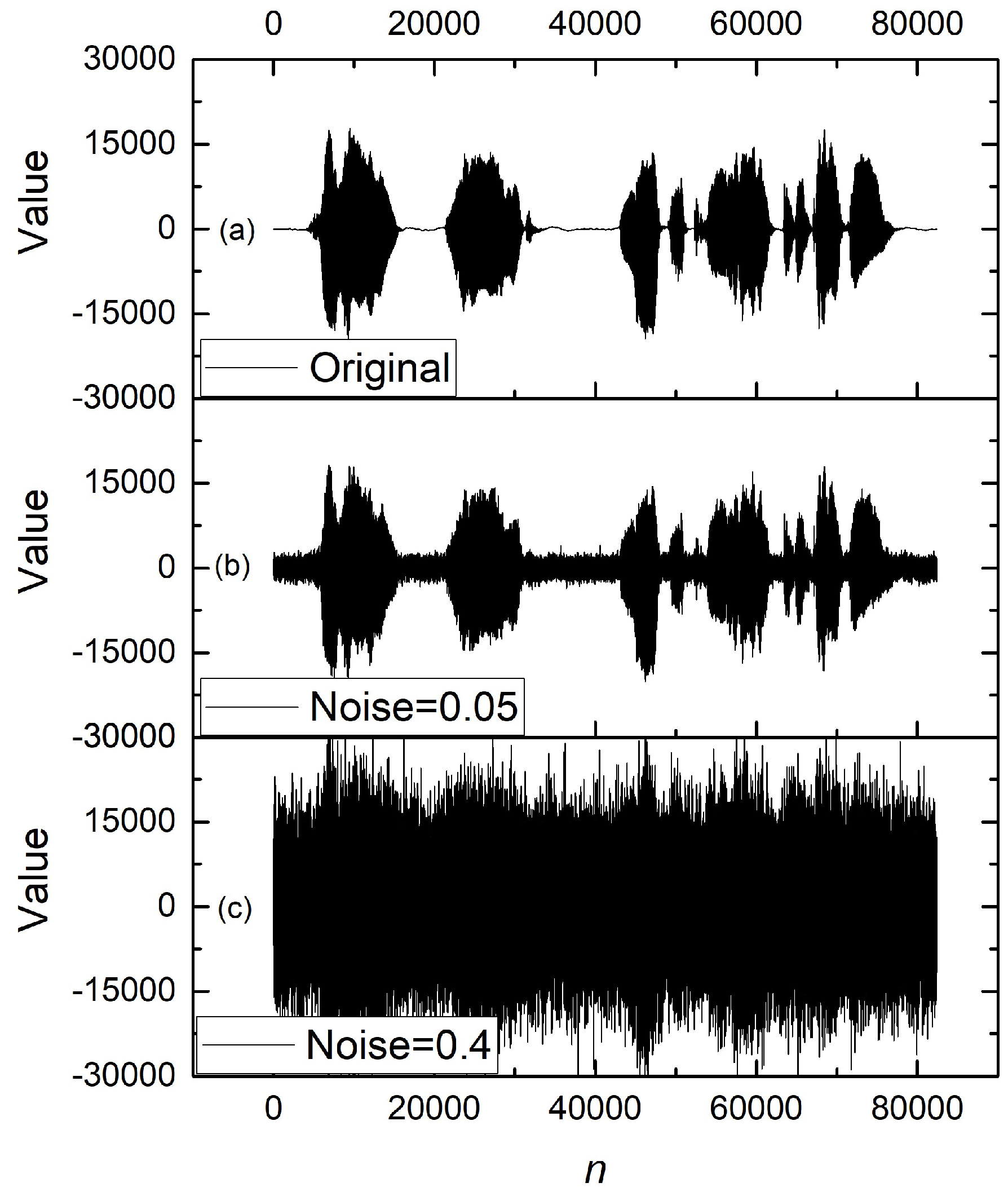
Figure 2.
The figure demonstrates the process of feature extraction from a time-series signal using a sliding window approach. The half-window size HW determines the number of time steps from the center to the edge of the window, specifying the range for extracting features around the current target signal value, shown as black squares. The corresponding features are derived from the noisy signal, represented by red circles, using values on both sides of the current point t. The green triangles indicate the model’s predictions based on these features, demonstrating the reconstruction of the signal despite the presence of noise.
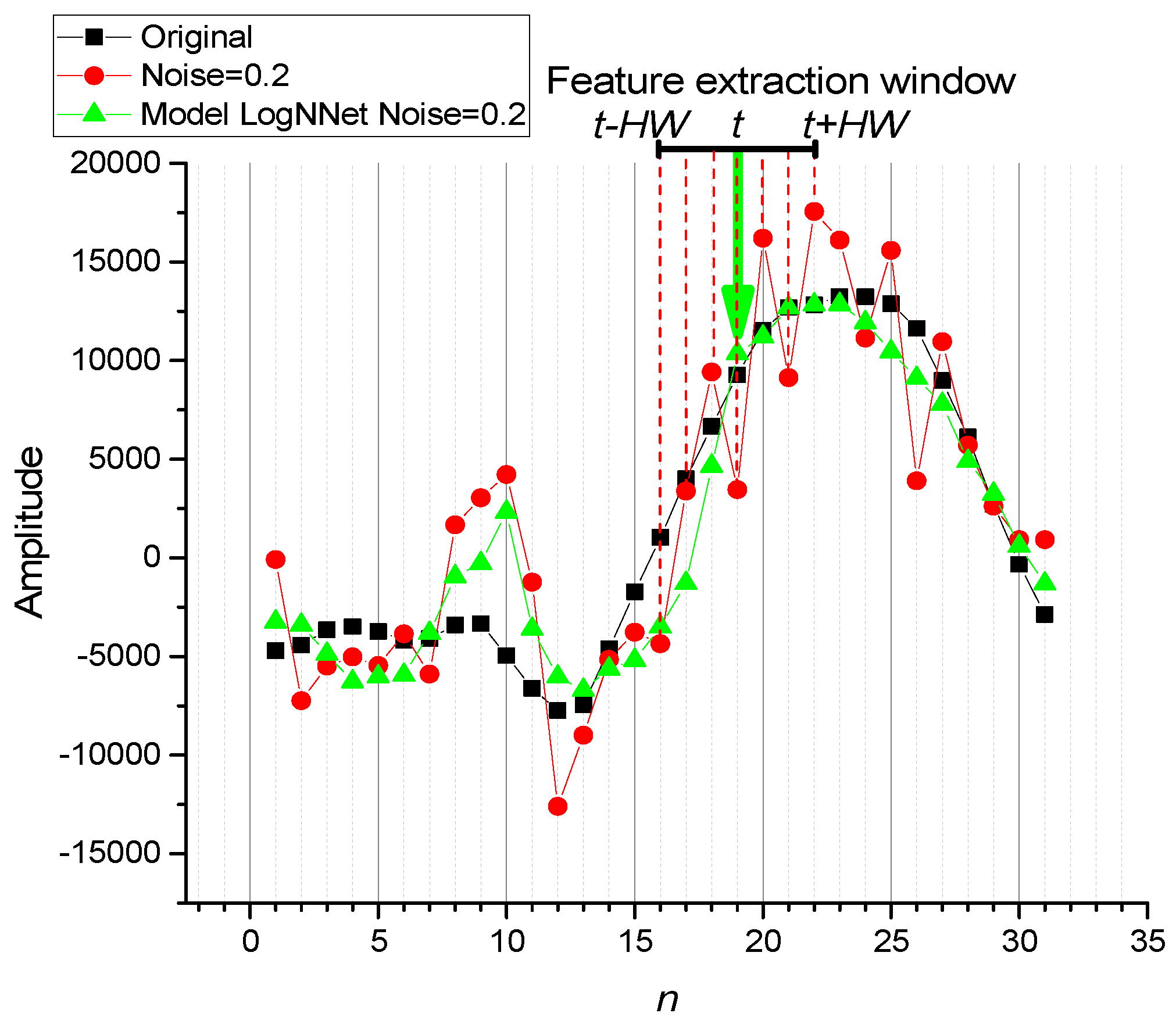
Figure 3.
Time series (black dots) with red numbers indicating the node degree calculated using the horizontal visibility graph algorithm. Arrows represent horizontal edges of the graph leading to the point n = 2.
Figure 3.
Time series (black dots) with red numbers indicating the node degree calculated using the horizontal visibility graph algorithm. Arrows represent horizontal edges of the graph leading to the point n = 2.
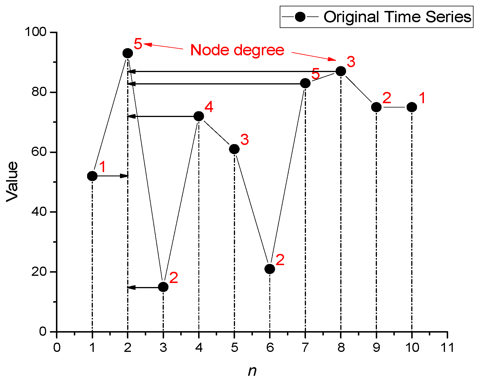
Figure 4.
Structure of LogNNet. The diagram illustrates the LogNNet workflow integrated with PSO optimization. The model consists of six stages: input normalization, chaotic reservoir computing, normalization of reservoir output, training of a classifier or regressor, PSO-based optimization of key parameters (e.g., chaotic weights, neuron count, training settings), and final testing. The PSO block, shown with a dashed red line, interacts with multiple stages, optimizing the network through feedback connections indicated by red arrows.
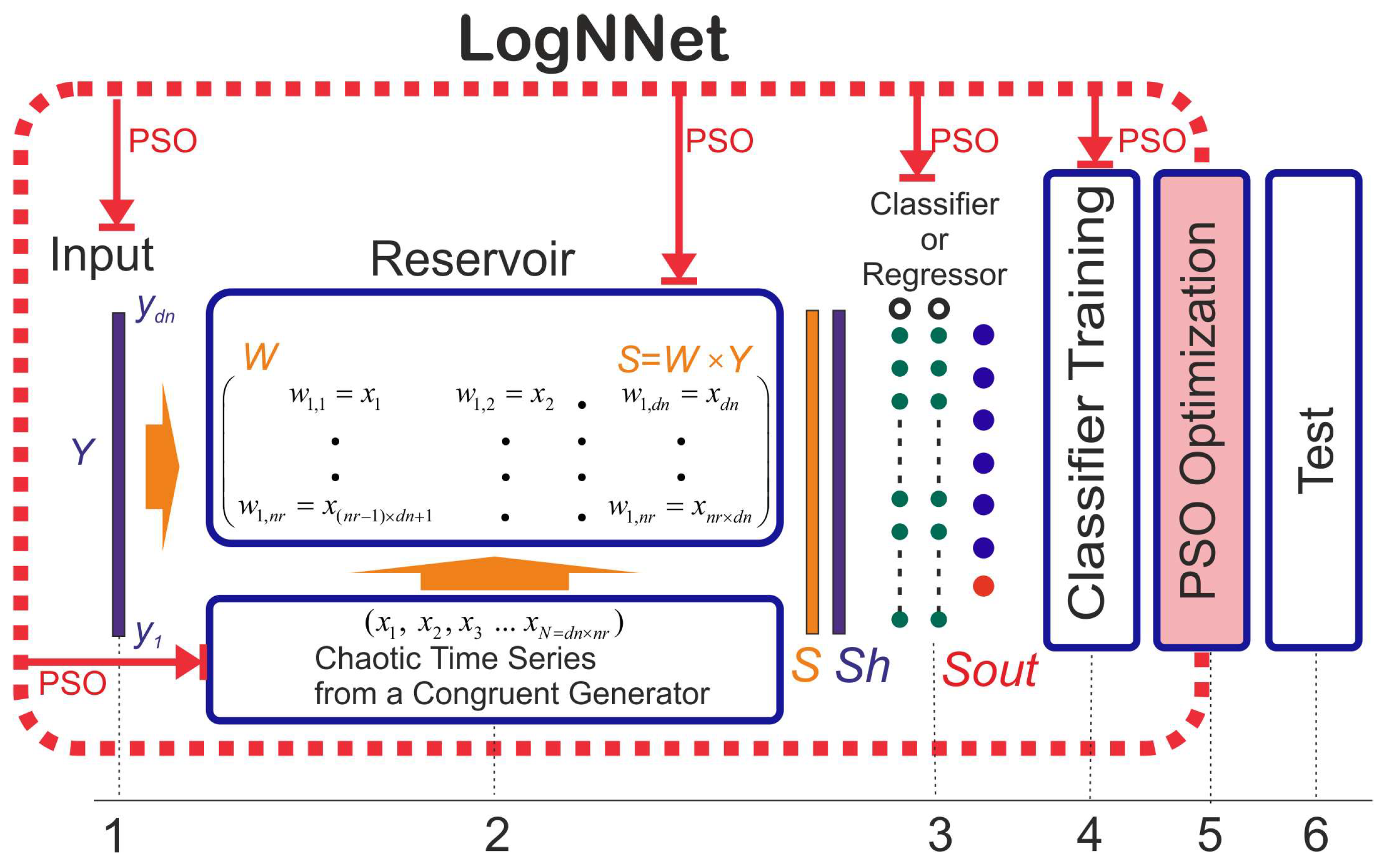
Figure 5.
(a) The effect of HVG features on reducing MAE (D_MAE, %) for LogNNet models with different numbers of features (HW = 1, 3, and 10) during testing on signals with various noise levels. (b) The percentage difference (DD_MAE) between the MAE values of LogNNet models with and without HVG features at different HW values (1, 3, 10).
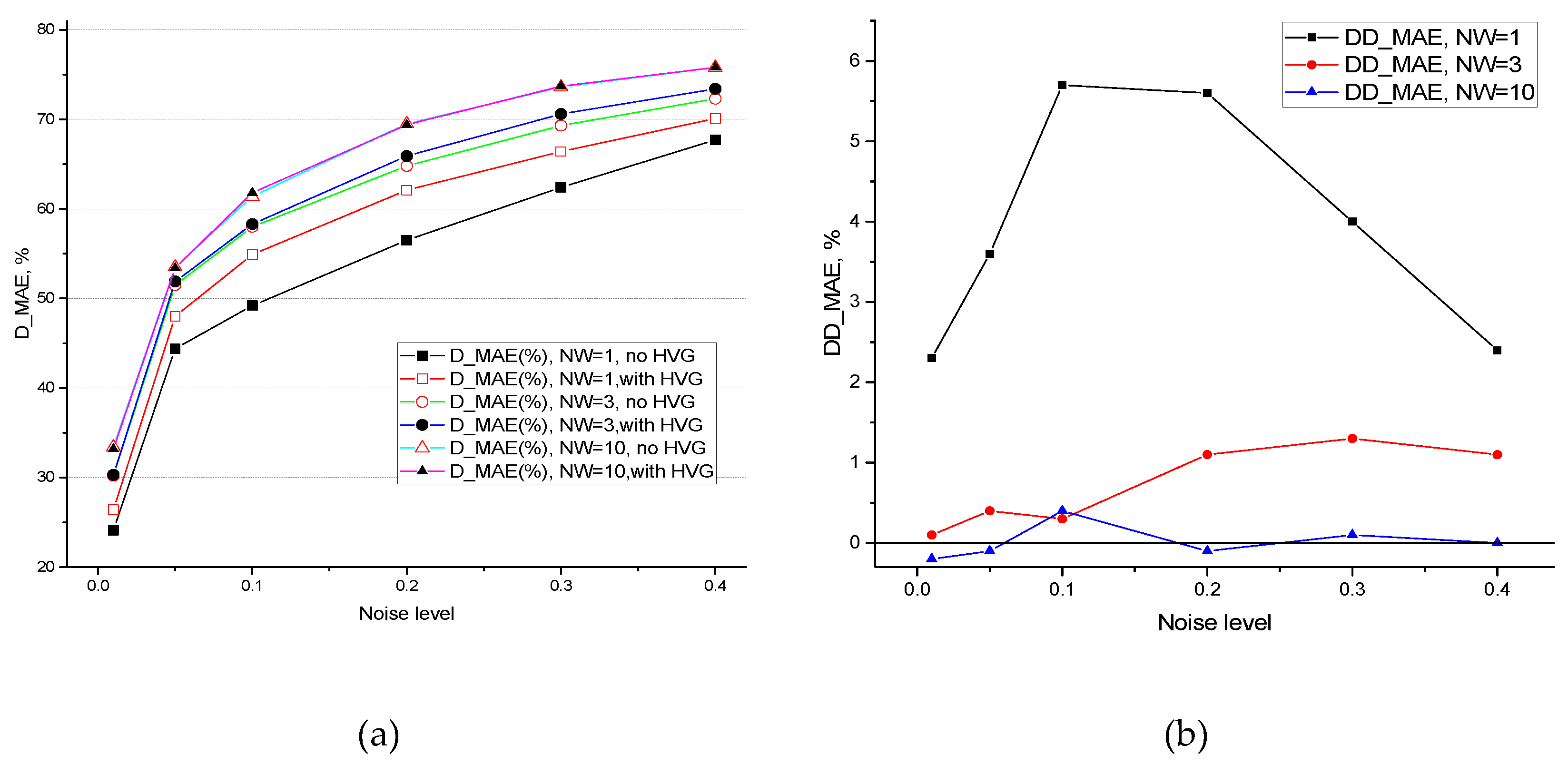
Figure 6.
Oscillograms of audio signals at different stages of processing: (a) original noise-free signal (MAE = 0), (b) signal with added noise at level 0.2 (MAE = 3176.4), (c) application of the LogNNet model without HVG features (HW = 1) with D_MAE = 56.5% (MAE = 1382), (d) application of the LogNNet model with HVG features (HW = 1) with D_MAE = 62.1% (MAE = 1204), (e) application of the LogNNet model without HVG features (HW = 10) with D_MAE = 69.5% (MAE = 967). As the number of features (HW) increases, the noise filtering quality improves, resulting in lower MAE.
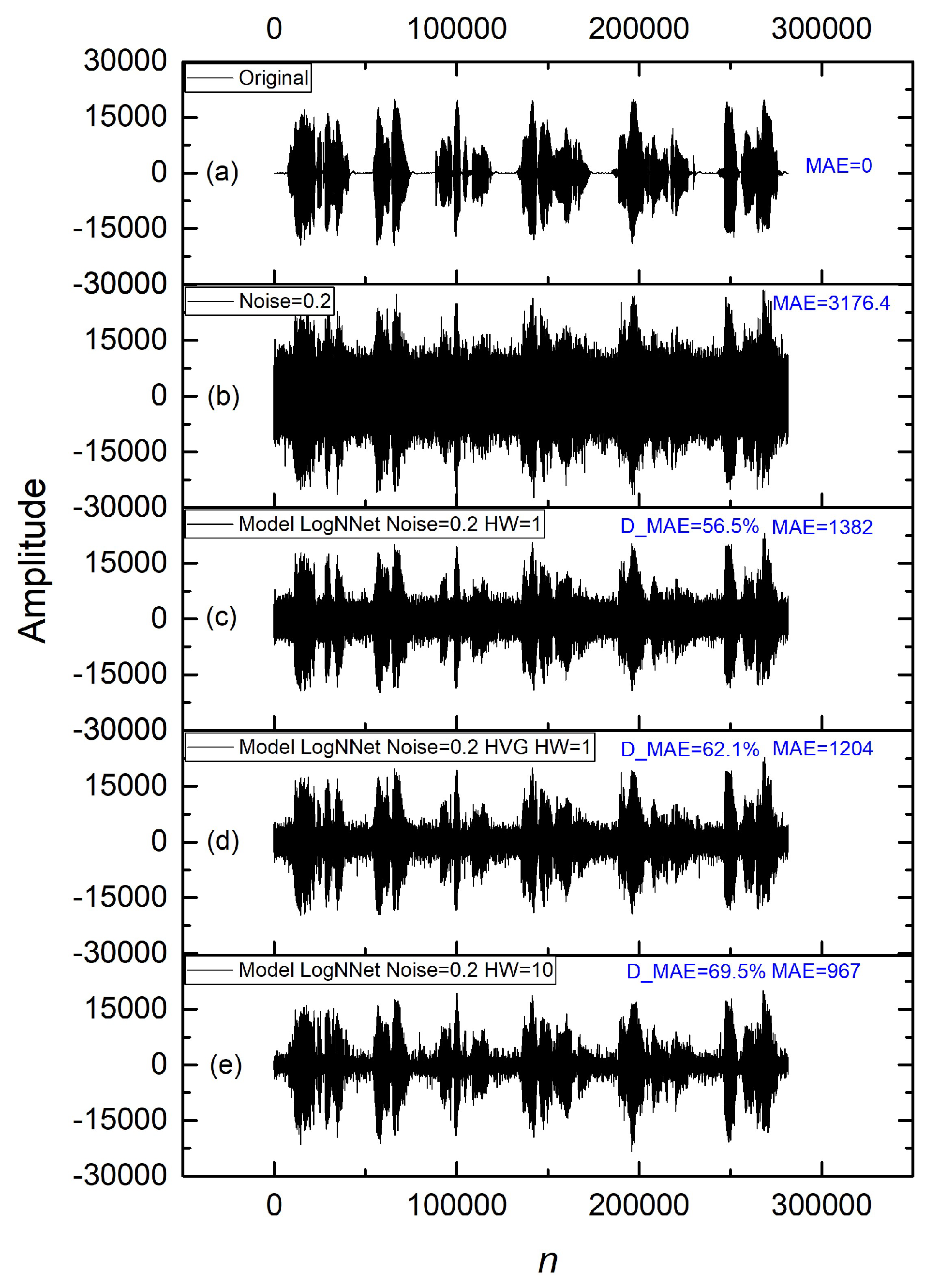
Figure 7.
Oscillograms of an audio signal with noise level 0.05: (a) noisy signal (MAE = 792.5), (b) restored signal using the LogNNet model (HW = 10) with HVG features (D_MAE = 53.5%, MAE = 368.9).
Figure 7.
Oscillograms of an audio signal with noise level 0.05: (a) noisy signal (MAE = 792.5), (b) restored signal using the LogNNet model (HW = 10) with HVG features (D_MAE = 53.5%, MAE = 368.9).
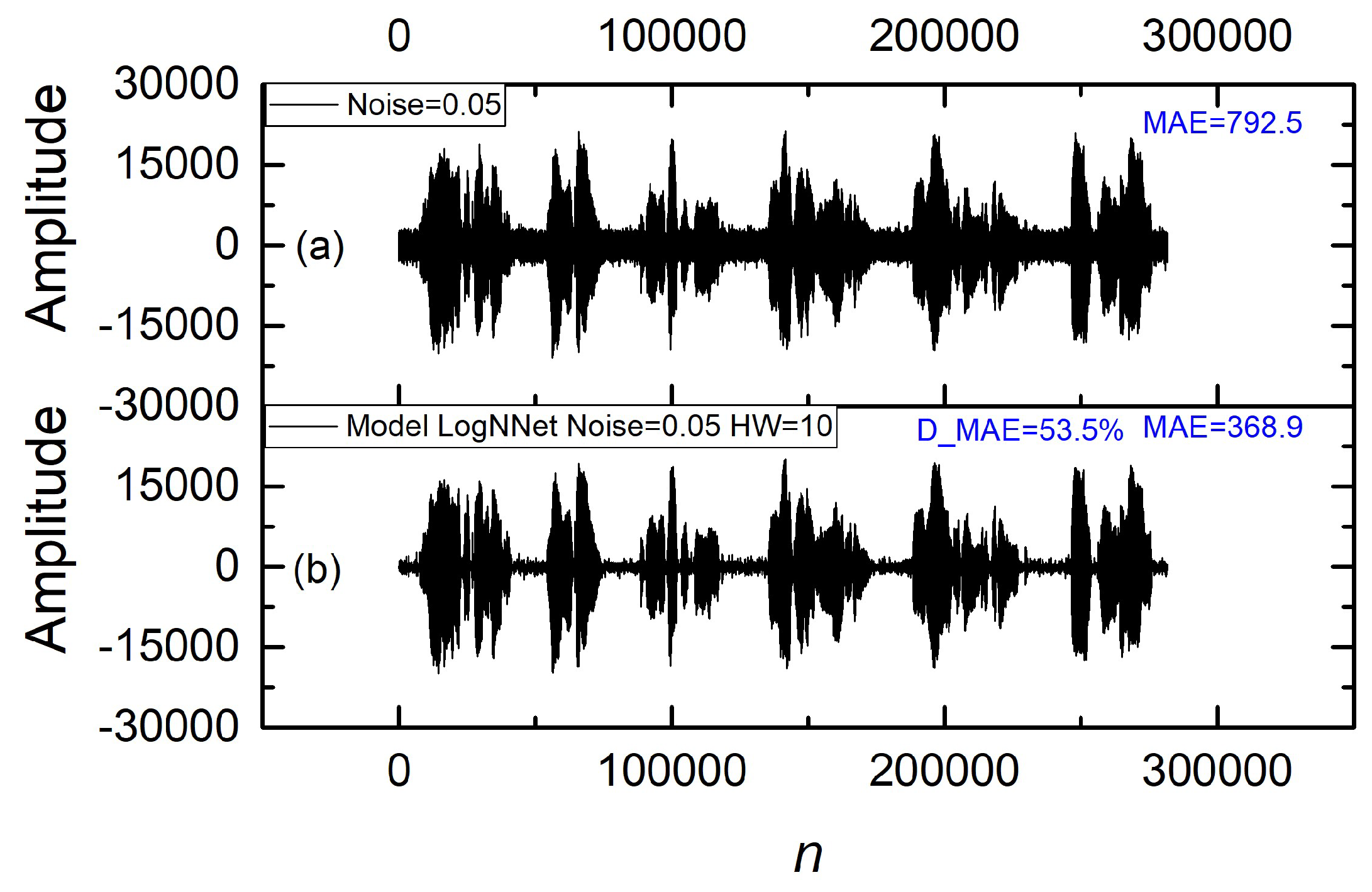

Table 1.
Coefficient of determination (R²) and mean absolute error (MAE) when comparing the original and noisy test audio signals at various noise levels.
Table 1.
Coefficient of determination (R²) and mean absolute error (MAE) when comparing the original and noisy test audio signals at various noise levels.
| Noise Level | R² Coefficient | MAE Coefficient |
|---|---|---|
| 0.01 | 0.997 | 158.6 |
| 0.05 | 0.925 | 792.5 |
| 0.1 | 0.703 | 1586.7 |
| 0.2 | <0 | 3176.4 |
| 0.3 | <0 | 4772.1 |
| 0.4 | <0 | 6358.9 |
Table 2.
Testing results of LogNNet models at various levels of audio signal noise based on R² and MAE metrics for models with HW = 1, without HVG application. Diagonal elements (in parentheses) represent cases with identical noise levels in training and test data.
Table 2.
Testing results of LogNNet models at various levels of audio signal noise based on R² and MAE metrics for models with HW = 1, without HVG application. Diagonal elements (in parentheses) represent cases with identical noise levels in training and test data.
| Model LogNNet HW = 1 |
R2 for test signal | MAE for test signal | ||||||||||
|---|---|---|---|---|---|---|---|---|---|---|---|---|
| 0.01 | 0.05 | 0.1 | 0.2 | 0.3 | 0.4 | 0.01 | 0.05 | 0.1 | 0.2 | 0.3 | 0.4 | |
| Noise = 0.01 | (0.998) | 0.934 | 0.714 | <0 | <0 | <0 | (120) | 734 | 1551 | 3186 | 4824 | 6450 |
| Noise = 0.05 | 0.989 | (0.971) | 0.845 | 0.143 | <0 | <0 | 239 | (440) | 1079 | 2682 | 4254 | 5779 |
| Noise = 0. 1 | 0.966 | 0.956 | (0.906) | 0.502 | <0 | <0 | 433 | 515 | (805) | 1964 | 3376 | 4771 |
| Noise = 0. 2 | 0.886 | 0.881 | 0.858 | (0.726) | 0.364 | <0 | 877 | 880 | 952 | (1382) | 2157 | 3144 |
| Noise = 0. 3 | 0.753 | 0.750 | 0.739 | 0.688 | (0.538) | 0.247 | 1240 | 1258 | 1290 | 1435 | (1796) | 2318 |
| Noise = 0. 4 | 0.596 | 0.595 | 0.590 | 0.575 | 0.517 | (0.385) | 1509 | 1518 | 1546 | 1614 | 1773 | (2053) |
Table 3.
Testing results of LogNNet models at various levels of audio signal noise based on R² and MAE metrics for models with HW = 1, with HVG application. Diagonal elements (in parentheses) represent cases with identical noise levels in training and test data.
Table 3.
Testing results of LogNNet models at various levels of audio signal noise based on R² and MAE metrics for models with HW = 1, with HVG application. Diagonal elements (in parentheses) represent cases with identical noise levels in training and test data.
| Model LogNNet with HVG HW = 1 |
R2 for test signal | MAE for test signal | ||||||||||
|---|---|---|---|---|---|---|---|---|---|---|---|---|
| 0.01 | 0.05 | 0.1 | 0.2 | 0.3 | 0.4 | 0.01 | 0.05 | 0.1 | 0.2 | 0.3 | 0.4 | |
| Noise = 0.01 | (0.998) | 0.932 | 0.708 | <0 | <0 | <0 | (116) | 750 | 1569 | 3211 | 4856 | 6488 |
| Noise = 0.05 | 0.989 | (0.975) | 0.843 | 0.086 | <0 | <0 | 243 | (412) | 1096 | 2773 | 4430 | 6052 |
| Noise = 0. 1 | 0.954 | 0.955 | (0.923) | 0.506 | <0 | <0 | 526 | 511 | (716) | 1957 | 3613 | 5348 |
| Noise = 0. 2 | 0.844 | 0.867 | 0.869 | (0.785) | 0.391 | <0 | 999 | 903 | 894 | (1204) | 2080 | 3253 |
| Noise = 0. 3 | 0.690 | 0.737 | 0.760 | 0.753 | (0.626) | 0.291 | 1452 | 1308 | 1233 | 1259 | (1601) | 2243 |
| Noise = 0. 4 | 0.484 | 0.576 | 0.622 | 0.653 | 0.617 | (0.479) | 1844 | 1655 | 1547 | 1485 | 1593 | (1903) |
Table 4.
Comparison of the effectiveness of LogNNet models in noise suppression (D_MAE) without HVG features and with their application for HW = 1. The table presents D_MAE values in percentage terms.
Table 4.
Comparison of the effectiveness of LogNNet models in noise suppression (D_MAE) without HVG features and with their application for HW = 1. The table presents D_MAE values in percentage terms.
| Model LogNNet HW = 1 |
D_MAE(%) for test signal (no HVG) |
D_MAE(%) for test signal (with HVG) |
||||||||||
|---|---|---|---|---|---|---|---|---|---|---|---|---|
| 0.01 | 0.05 | 0.1 | 0.2 | 0.3 | 0.4 | 0.01 | 0.05 | 0.1 | 0.2 | 0.3 | 0.4 | |
| Noise = 0.01 | 24.1 | 7.4 | 2.2 | -0.3 | -1.1 | -1.4 | 26.4 | 5.3 | 1.1 | -1.1 | -1.8 | -2 |
| Noise = 0.05 | -50.9 | 44.4 | 31.9 | 15.6 | 10.8 | 9.1 | -53.7 | 48 | 30.9 | 12.7 | 7.2 | 4.8 |
| Noise = 0. 1 | -173.3 | 35 | 49.2 | 38.2 | 29.2 | 25 | -232 | 35.4 | 54.9 | 38.4 | 24.3 | 15.9 |
| Noise = 0. 2 | -453.2 | -11 | 40 | 56.5 | 54.8 | 50.5 | -530.1 | -14 | 43.6 | 62.1 | 56.4 | 48.8 |
| Noise = 0. 3 | -682.4 | -58.8 | 18.6 | 54.8 | 62.4 | 63.5 | -815.7 | -65.1 | 22.3 | 60.3 | 66.4 | 64.7 |
| Noise = 0. 4 | -851.5 | -91.7 | 2.5 | 49.2 | 62.8 | 67.7 | -1063 | -108.9 | 2.5 | 53.2 | 66.6 | 70.1 |
Table 5.
Comparison of the effectiveness of LogNNet models without HVG features and with their application for HW = 3. The table presents D_MAE values in percentage terms.
Table 5.
Comparison of the effectiveness of LogNNet models without HVG features and with their application for HW = 3. The table presents D_MAE values in percentage terms.
| Model LogNNet HW = 3 |
D_MAE(%) for test signal (no HVG) |
D_MAE(%) for test signal (with HVG) |
||||||||||
|---|---|---|---|---|---|---|---|---|---|---|---|---|
| 0.01 | 0.05 | 0.1 | 0.2 | 0.3 | 0.4 | 0.01 | 0.05 | 0.1 | 0.2 | 0.3 | 0.4 | |
| Noise = 0.01 | 30.2 | 9.3 | 4.4 | 3.1 | 3 | 3 | 30.3 | 8.4 | 2.9 | 0.1 | -0.8 | -1.2 |
| Noise = 0.05 | -36.7 | 51.5 | 36 | 19.8 | 16 | 14.4 | -41.5 | 51.9 | 35.6 | 23.3 | 21 | 20.3 |
| Noise = 0. 1 | -150 | 42.6 | 58 | 40.8 | 27.5 | 20.4 | -150.1 | 43.8 | 58.3 | 39.7 | 31.5 | 28 |
| Noise = 0. 2 | -324.6 | 13.5 | 52.4 | 64.8 | 58.1 | 47.1 | -340.3 | 11.3 | 52.3 | 65.9 | 59.1 | 49.5 |
| Noise = 0. 3 | -504.6 | -22.1 | 37.4 | 64.4 | 69.3 | 69 | -557 | -27.4 | 36.4 | 65.5 | 70.6 | 69.8 |
| Noise = 0. 4 | -689.7 | -56.4 | 21.9 | 59.6 | 69.5 | 72.3 | -735.7 | -59.3 | 21.9 | 60.5 | 70.7 | 73.4 |
Table 6.
Comparison of the effectiveness of LogNNet models without HVG features and with their application for HW = 10. The table presents D_MAE values in percentage terms.
Table 6.
Comparison of the effectiveness of LogNNet models without HVG features and with their application for HW = 10. The table presents D_MAE values in percentage terms.
| Model LogNNet HW = 10 |
D_MAE(%) for test signal (no HVG) |
D_MAE(%) for test signal (with HVG) |
||||||||||
|---|---|---|---|---|---|---|---|---|---|---|---|---|
| 0.01 | 0.05 | 0.1 | 0.2 | 0.3 | 0.4 | 0.01 | 0.05 | 0.1 | 0.2 | 0.3 | 0.4 | |
| Noise = 0.01 | 33.4 | 11 | 5.8 | 3.7 | 3.4 | 3.4 | 33.2 | 11.7 | 6.5 | 4.3 | 3.7 | 3.3 |
| Noise = 0.05 | -47.5 | 53.5 | 41.5 | 28 | 24.1 | 22 | -51.1 | 53.4 | 40.6 | 26 | 22.8 | 21.8 |
| Noise = 0. 1 | -136.2 | 46.2 | 61.4 | 46.4 | 38.9 | 35.9 | -142.5 | 45.5 | 61.8 | 44.4 | 34.4 | 29.8 |
| Noise = 0. 2 | -308 | 16.8 | 55.5 | 69.5 | 63.2 | 54.9 | -302.1 | 18 | 55.7 | 69.4 | 63.3 | 56 |
| Noise = 0. 3 | -462.8 | -12.8 | 42.6 | 69.1 | 73.6 | 71.7 | -424.1 | -7.3 | 44.3 | 69.1 | 73.7 | 72.7 |
| Noise = 0. 4 | -594.8 | -38.7 | 30.3 | 64.8 | 73.9 | 75.8 | -584.6 | -37.3 | 30.6 | 64.5 | 73.8 | 75.8 |
Table 7.
Results of cascading LogNNet models without HVG features and with HW = 10. The table shows D_MAE values as a percentage relative to the initial noisy signal.
Table 7.
Results of cascading LogNNet models without HVG features and with HW = 10. The table shows D_MAE values as a percentage relative to the initial noisy signal.
| Model LogNNet HW = 10 |
MAE for Test Signal (by Number of Iterations) | D_MAE (%) for Test Signal (by Number of Iterations) | ||||
|---|---|---|---|---|---|---|
| 1 | 2 | 3 | 1 | 2 | 3 | |
| Noise = 0.01 | 105 (Noise = 0.01) | - | - | 33.4 | - | - |
| Noise = 0.05 | 368 (Noise = 0.05) | 359 (Noise = 0.05) | 358 (Noise = 0.01) | 53.5 | 54.7 | 54.8 |
| Noise = 0. 1 | 612 (Noise = 0.1) | 575 (Noise = 0.05) | 574 (Noise = 0.01) | 61.4 | 63.8 | 63.8 |
| Noise = 0. 2 | 967 (Noise = 0.2) | 887 (Noise = 0.1) | 886 (Noise = 0.01) | 69.6 | 72.1 | 72.1 |
| Noise = 0. 3 | 1261 (Noise = 0.3) | 1193 (Noise = 0.1) | 1192 (Noise = 0.05) | 73.6 | 75 | 75 |
| Noise = 0. 4 | 1538 (Noise = 0.4) | 1360 (Noise = 0.2) | 1355 (Noise = 0.05) | 75.8 | 78.6 | 78.7 |
Disclaimer/Publisher’s Note: The statements, opinions and data contained in all publications are solely those of the individual author(s) and contributor(s) and not of MDPI and/or the editor(s). MDPI and/or the editor(s) disclaim responsibility for any injury to people or property resulting from any ideas, methods, instructions or products referred to in the content. |
© 2025 by the authors. Licensee MDPI, Basel, Switzerland. This article is an open access article distributed under the terms and conditions of the Creative Commons Attribution (CC BY) license (http://creativecommons.org/licenses/by/4.0/).
Copyright: This open access article is published under a Creative Commons CC BY 4.0 license, which permit the free download, distribution, and reuse, provided that the author and preprint are cited in any reuse.


