

Submitted:
30 December 2024
Posted:
03 January 2025
You are already at the latest version
Abstract
This paper presents an open-source time dependent three-dimensional scalar photorefractive beam propagation model (PRProp3D) based on the well-known split step method. The angular spectrum method is used for the diffractive steps and the nonlinearities accumulated at the end of each diffractive step are applied using spatially varying phase screens. Comparisons with previously published experimental results are given for image amplification and photorefractive amplified scattering (fanning). Artifacts can be mitigated by use of step sizes less than 5~10 micrometers and by careful choice of the transverse computation grid size to ensure adequate sampling. The occurrence of wraparound effects associated with the use of discrete Fourier transforms is discussed.
Keywords:
1. Introduction
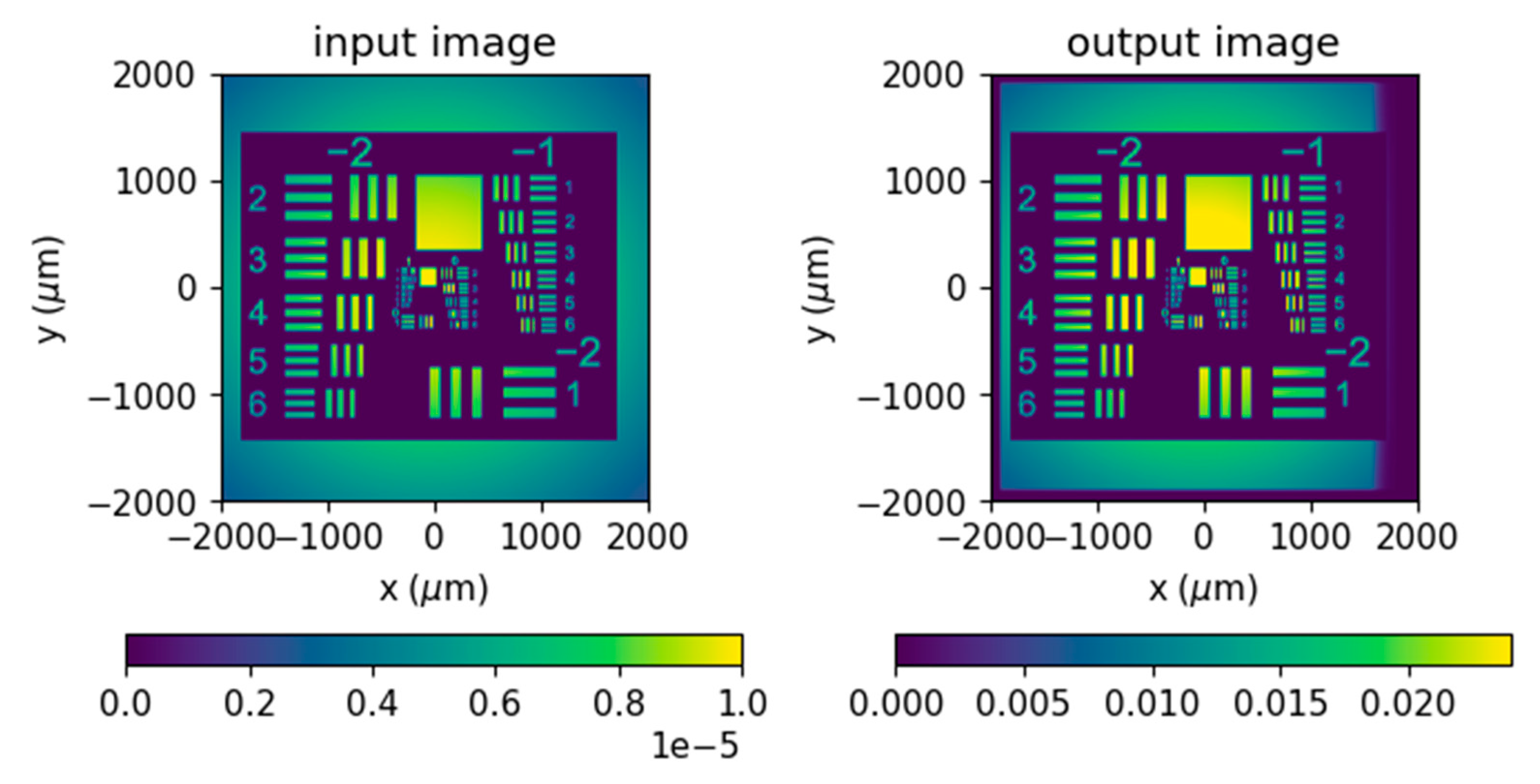
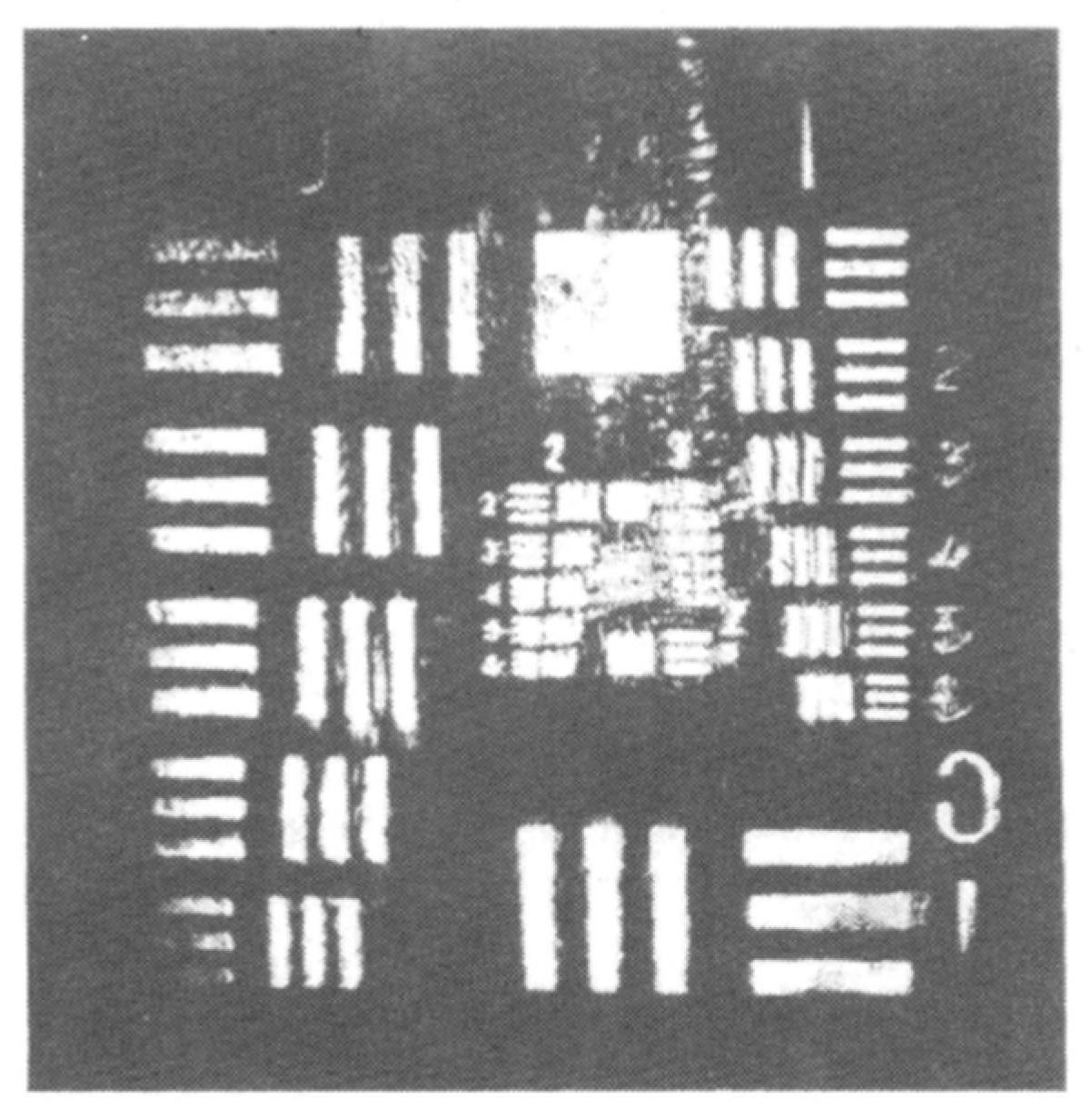
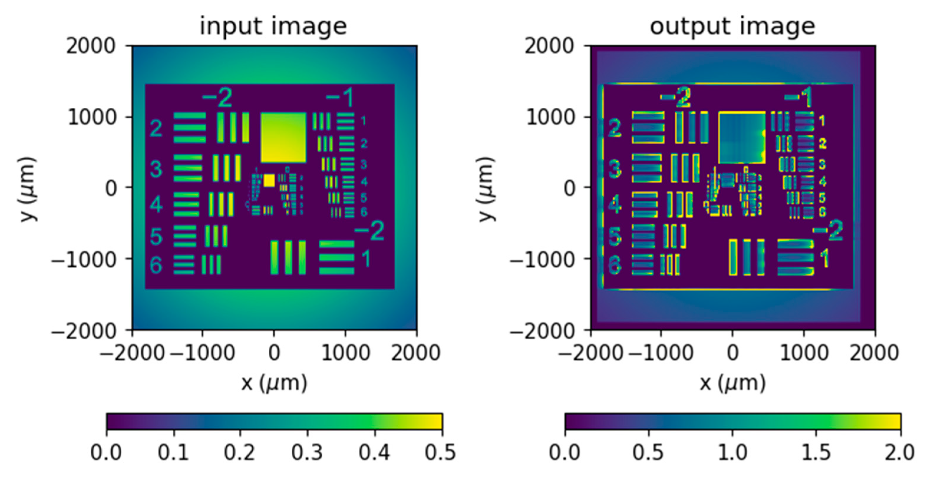
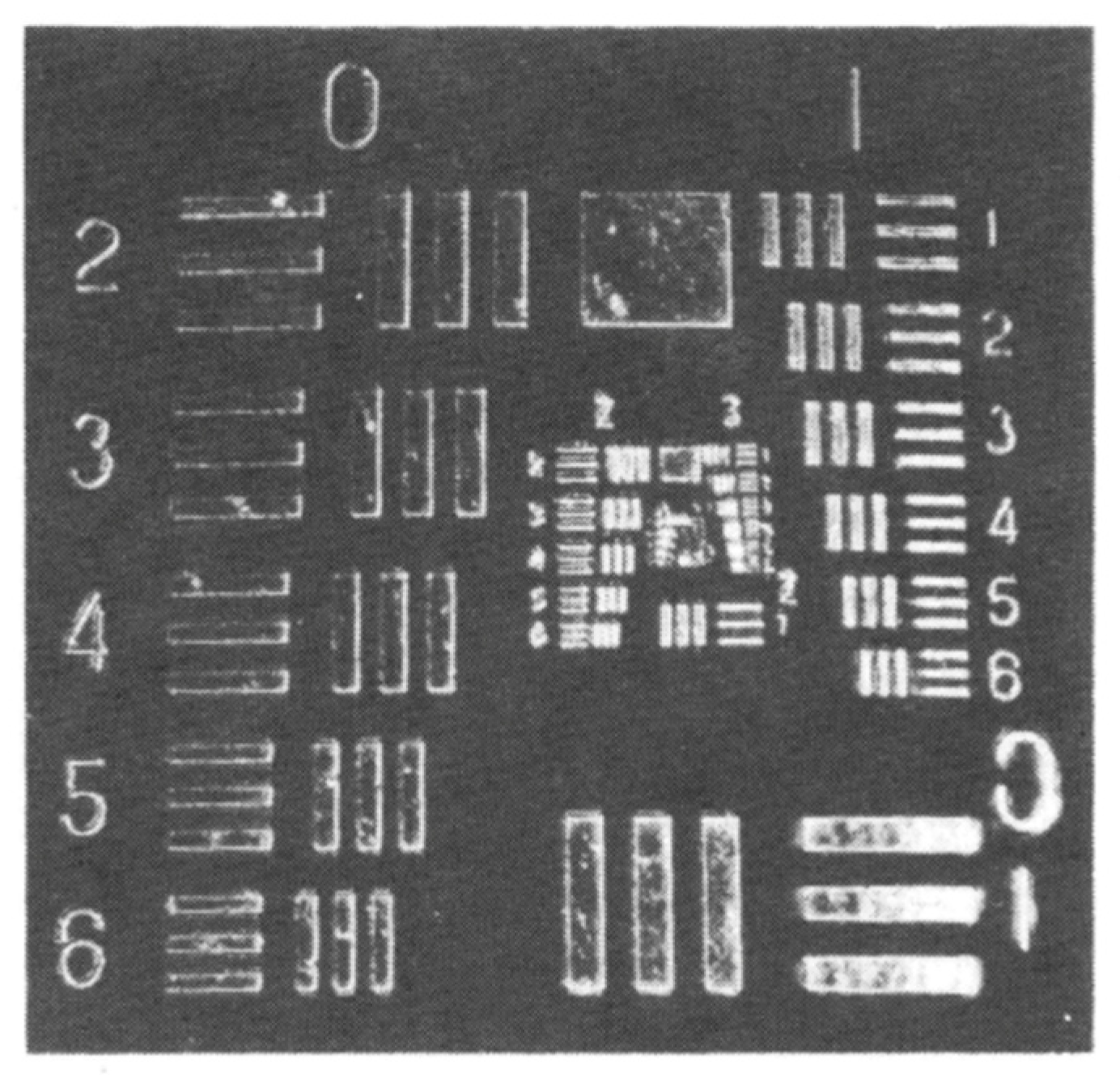
- Image amplification with comparison to experimental data published by Fainman et al.[16]
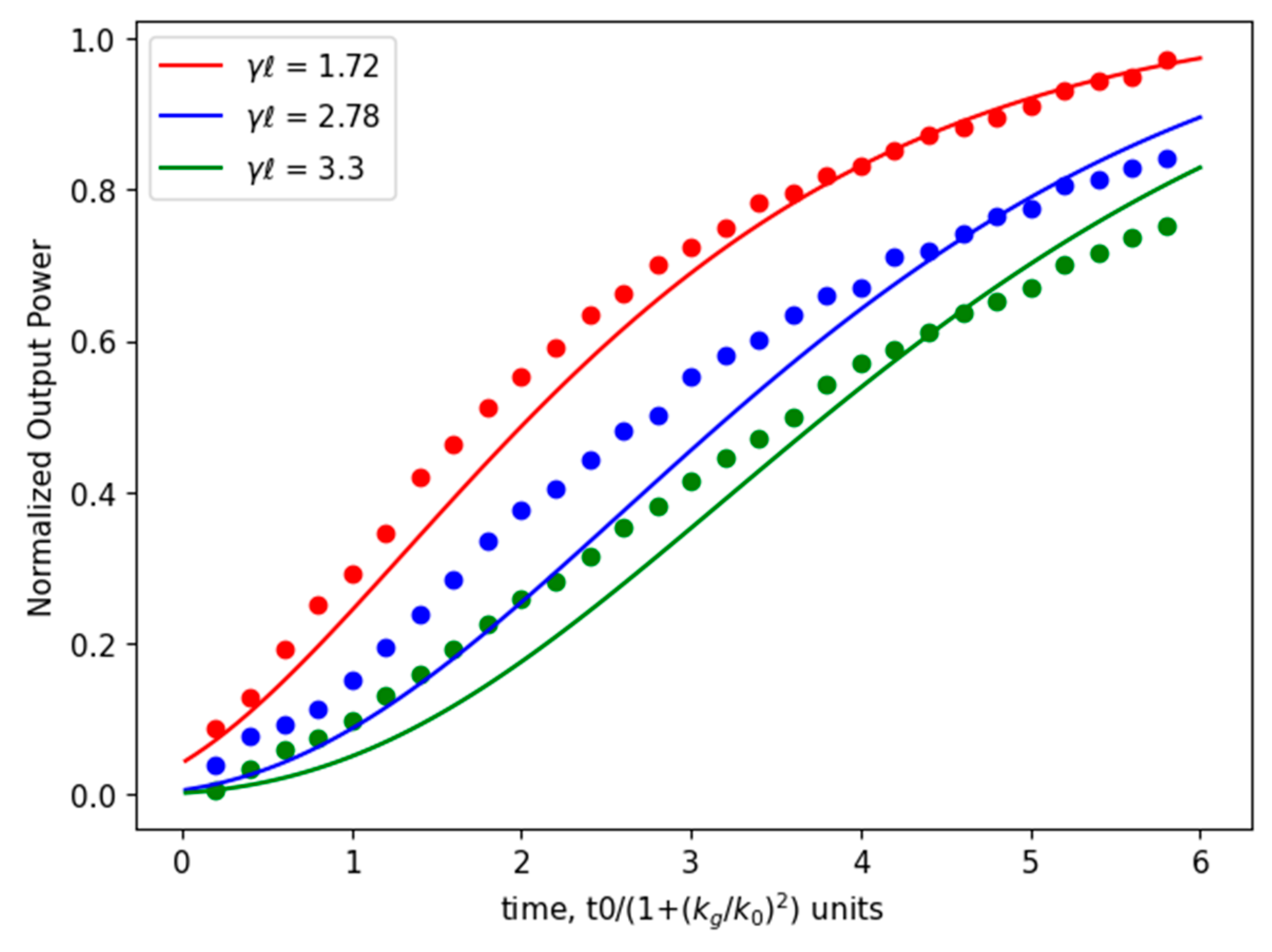
- Time dependence with comparison to high gain beam amplification experiments by Fischer et al[18].
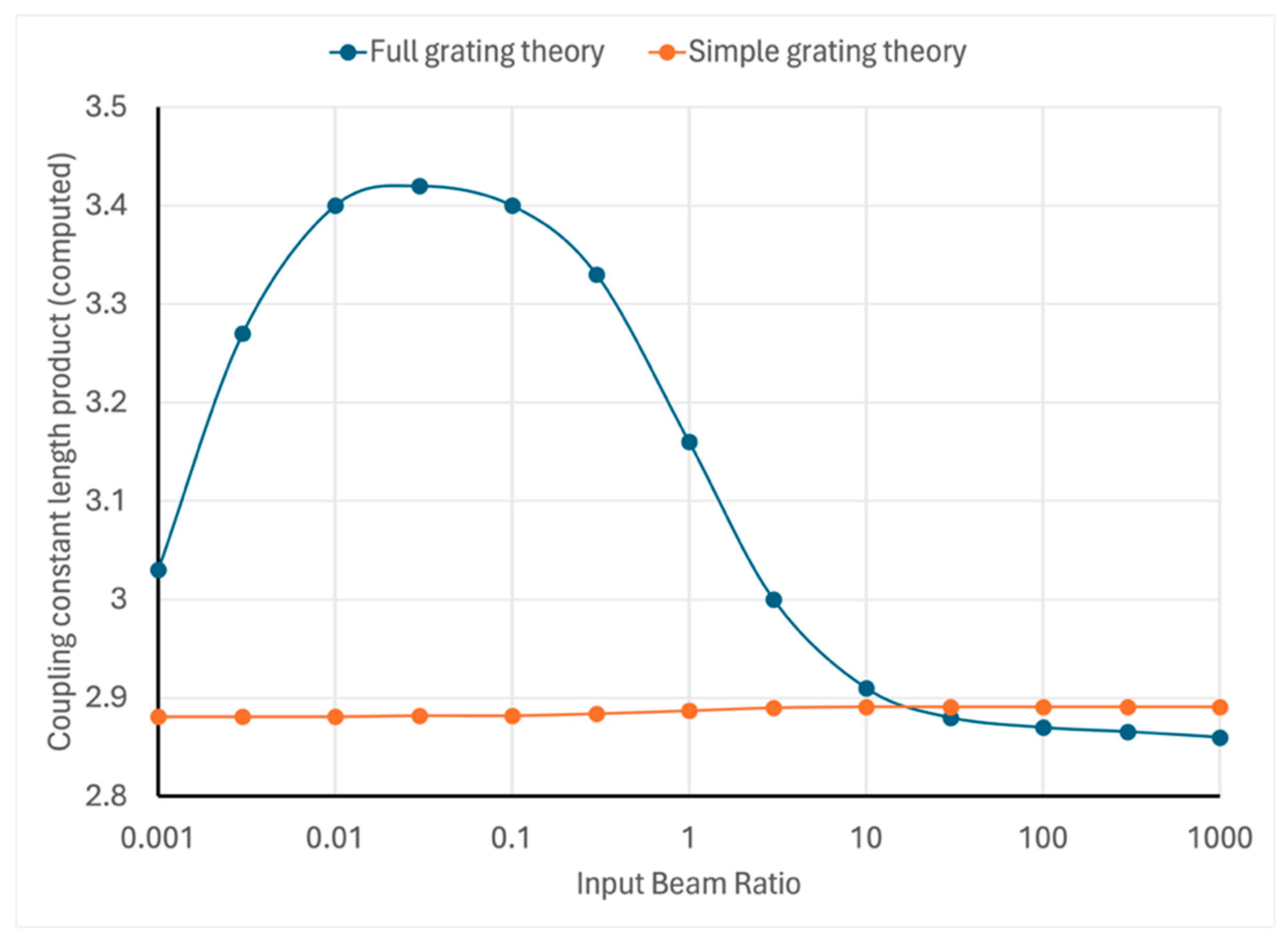
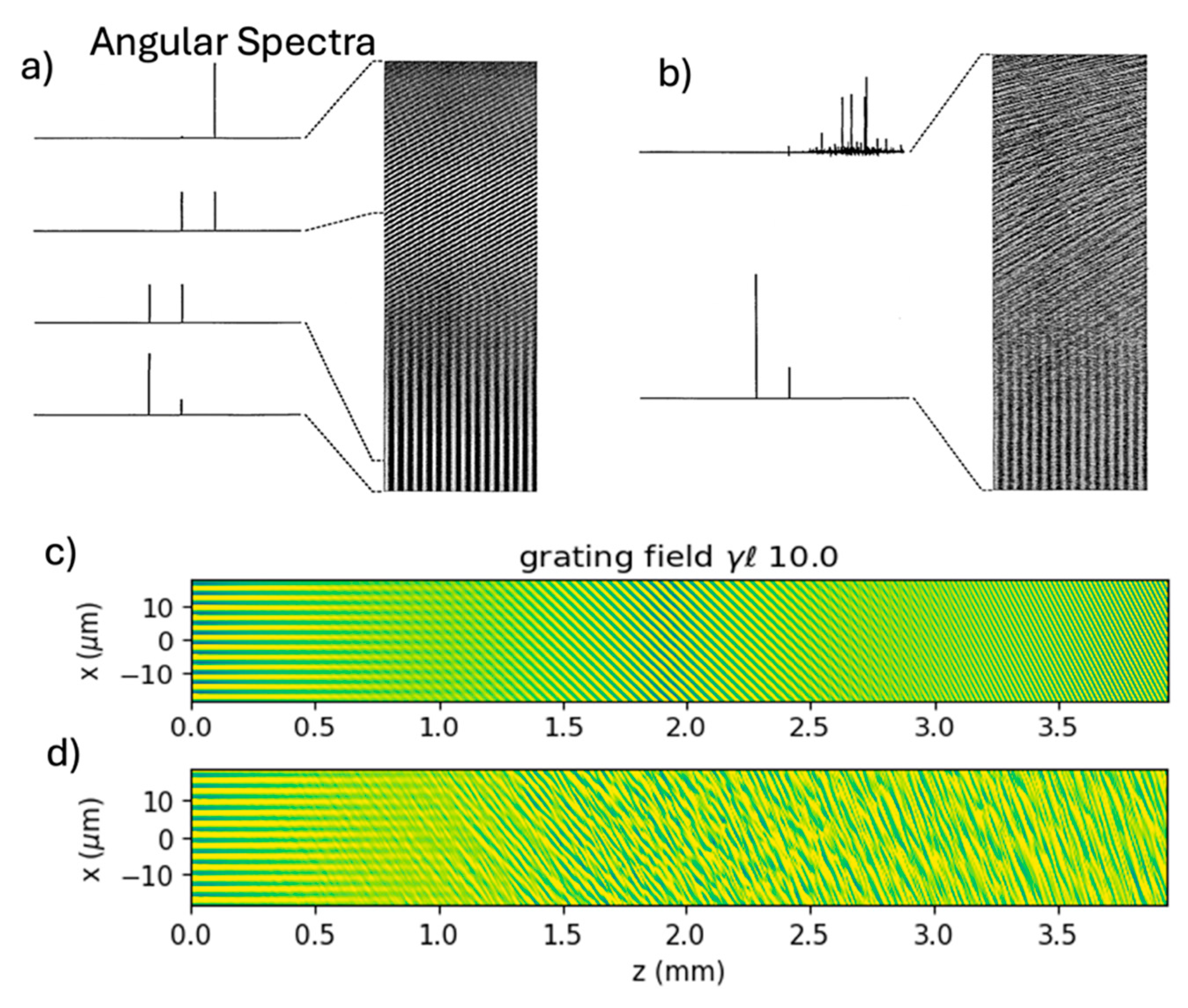
- Theoretical appearance of high order diffraction at high gain described by Brown and Valley[14]
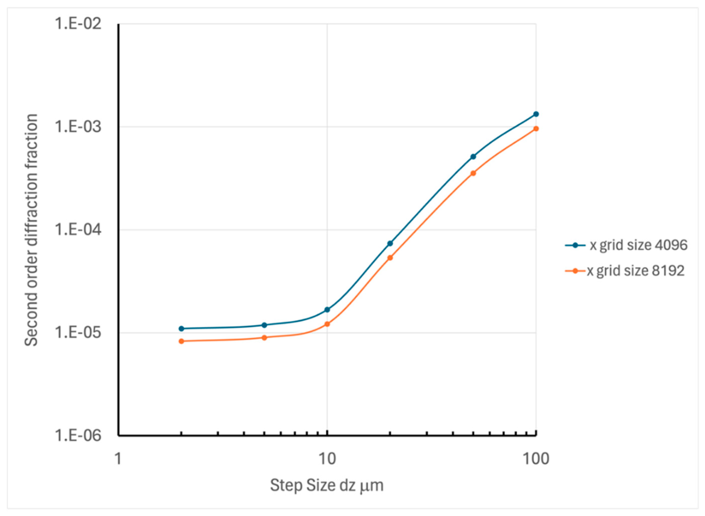
- The appearance of excess high order diffraction over interaction lengths nominally in the Bragg regime. This effect decreases with decreasing longitudinal step size but does not tend to zero.
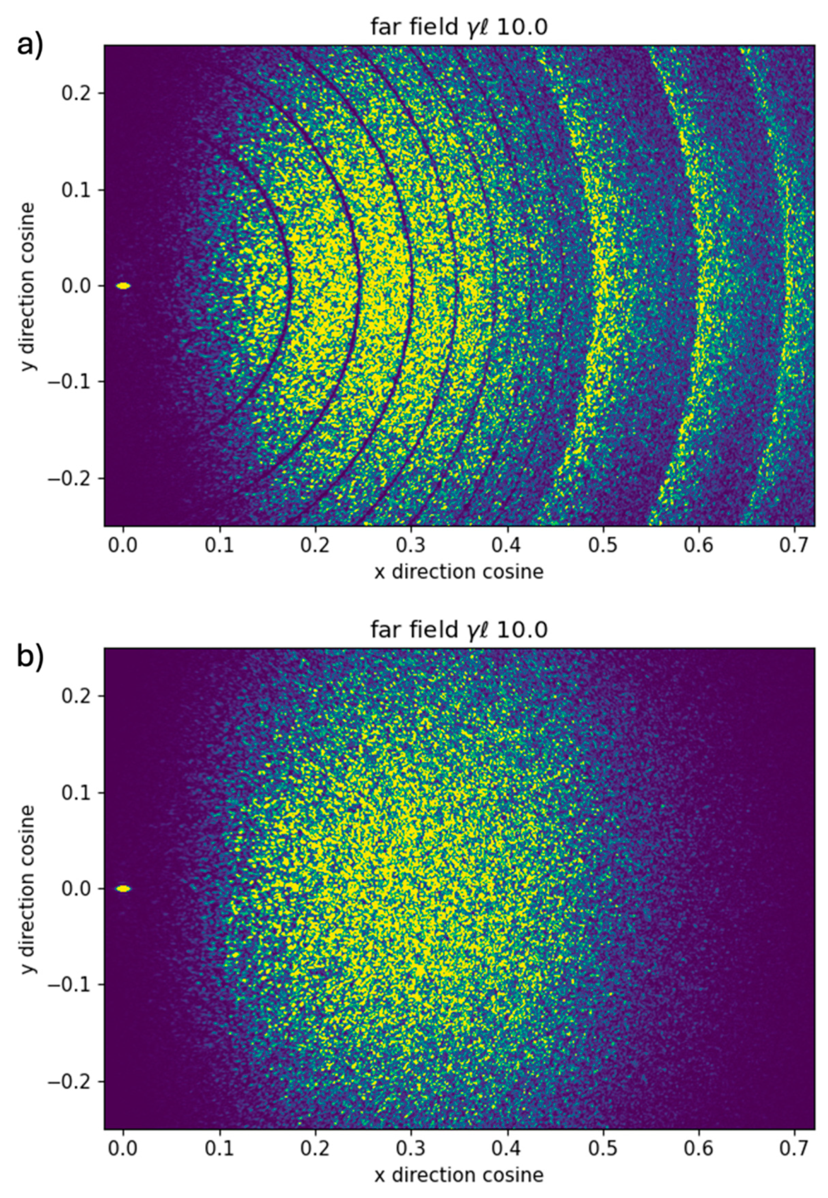
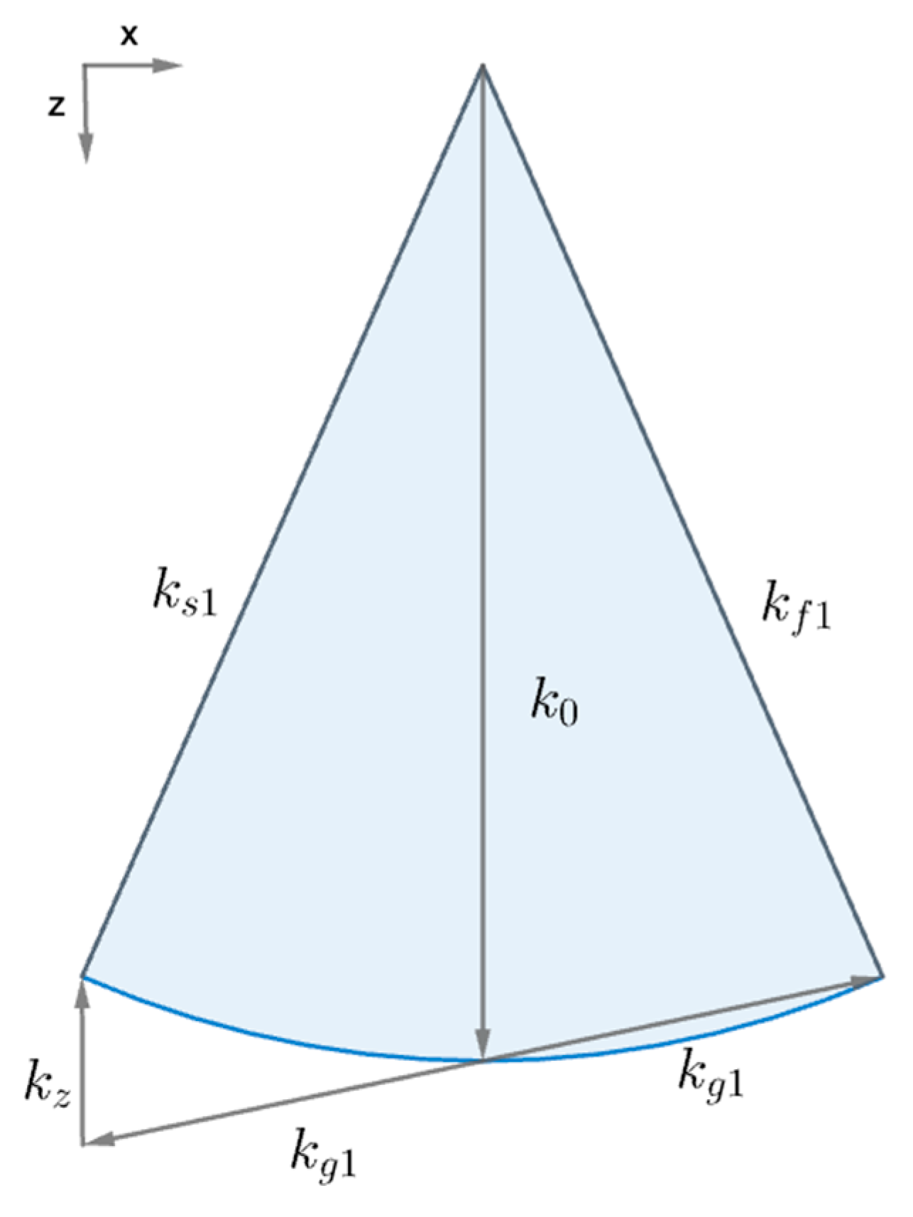
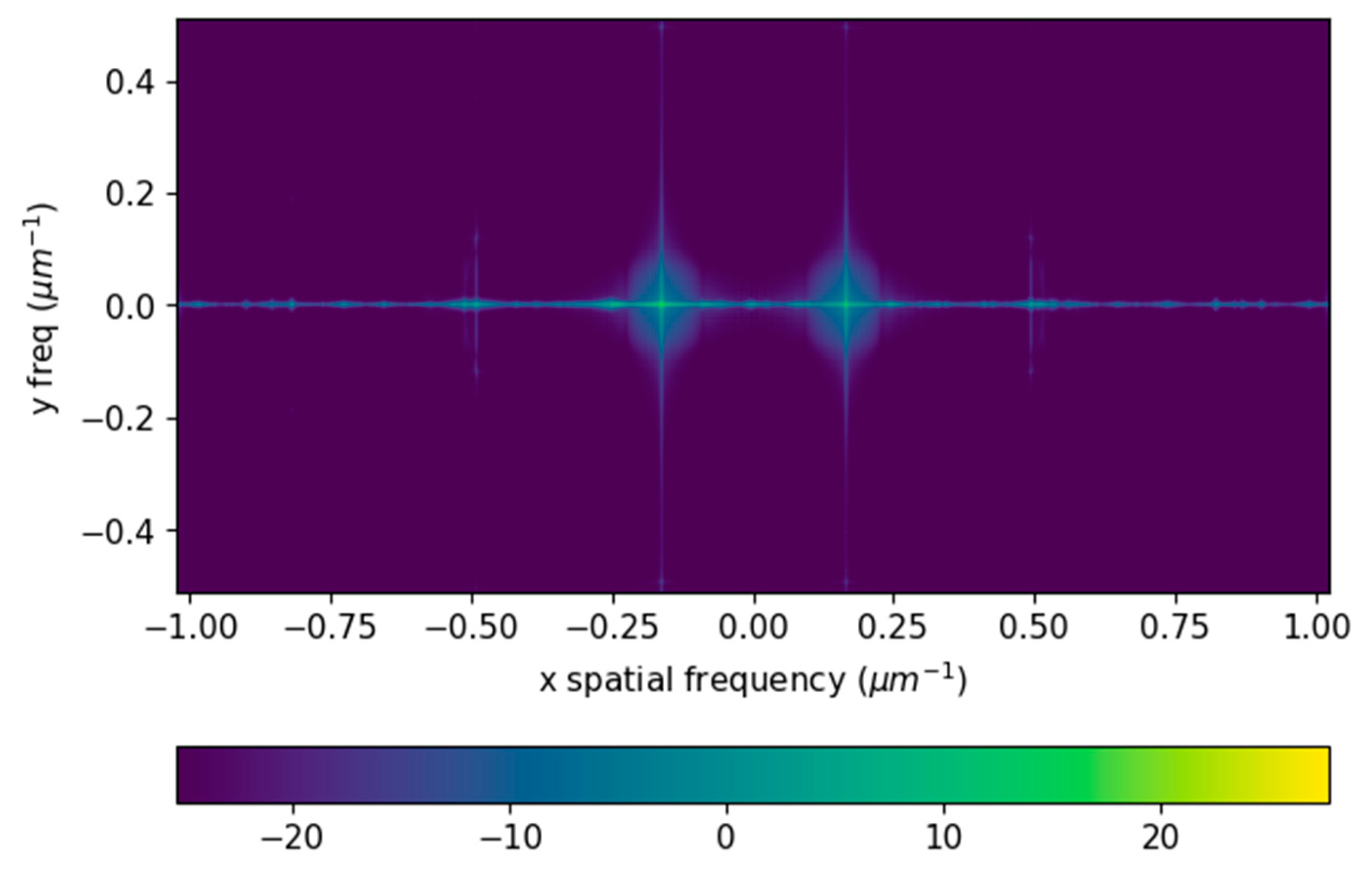
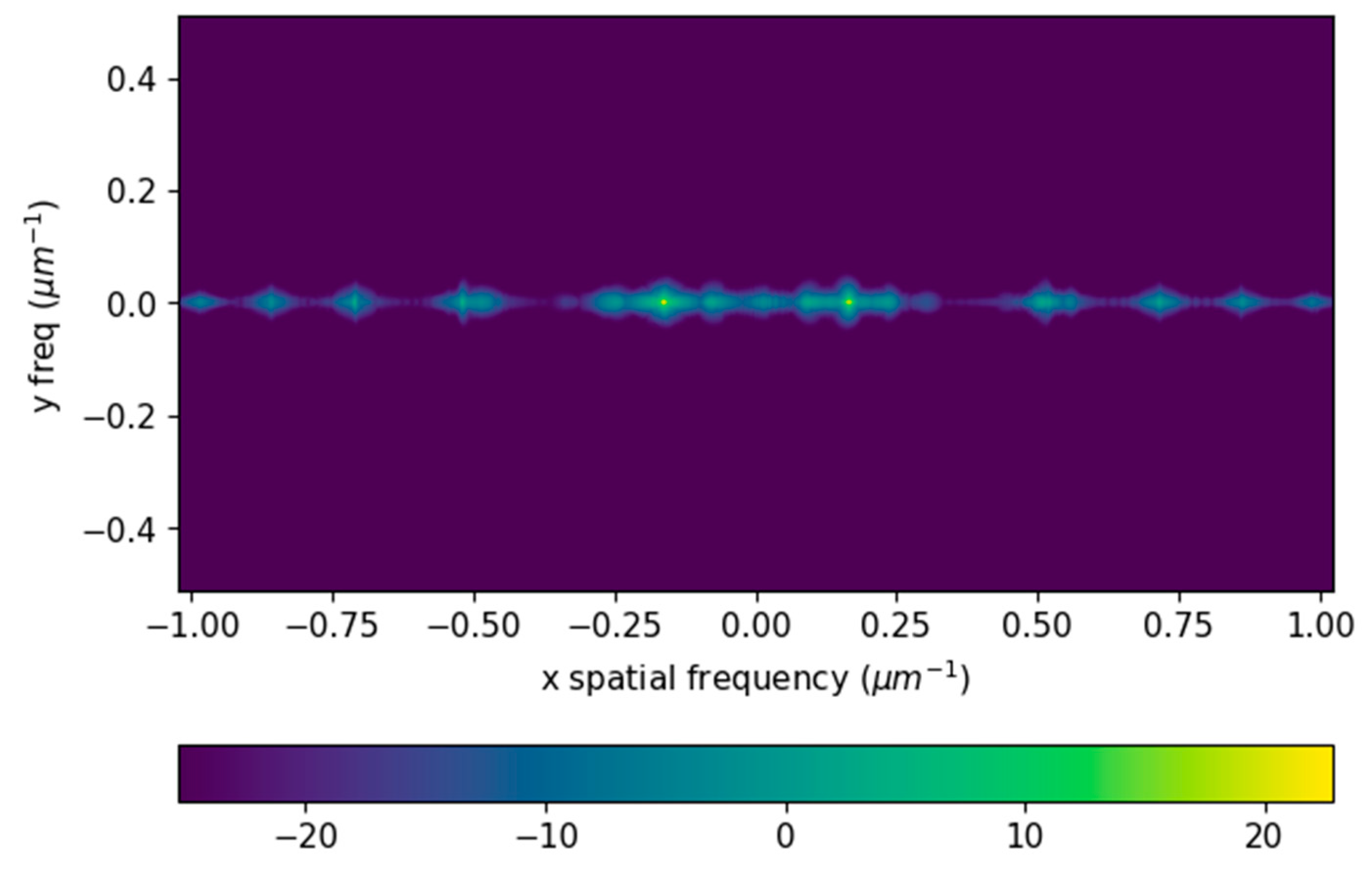
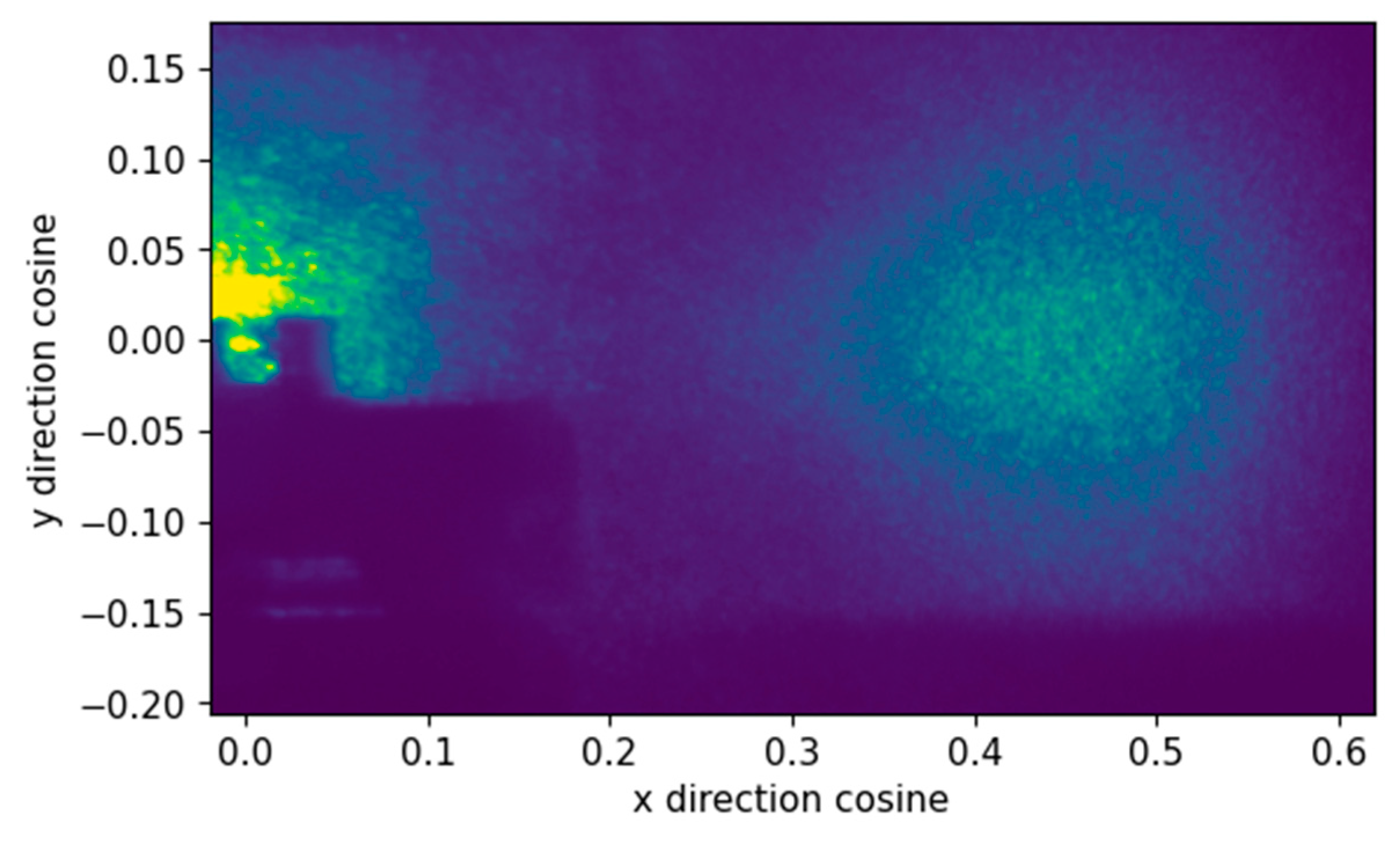
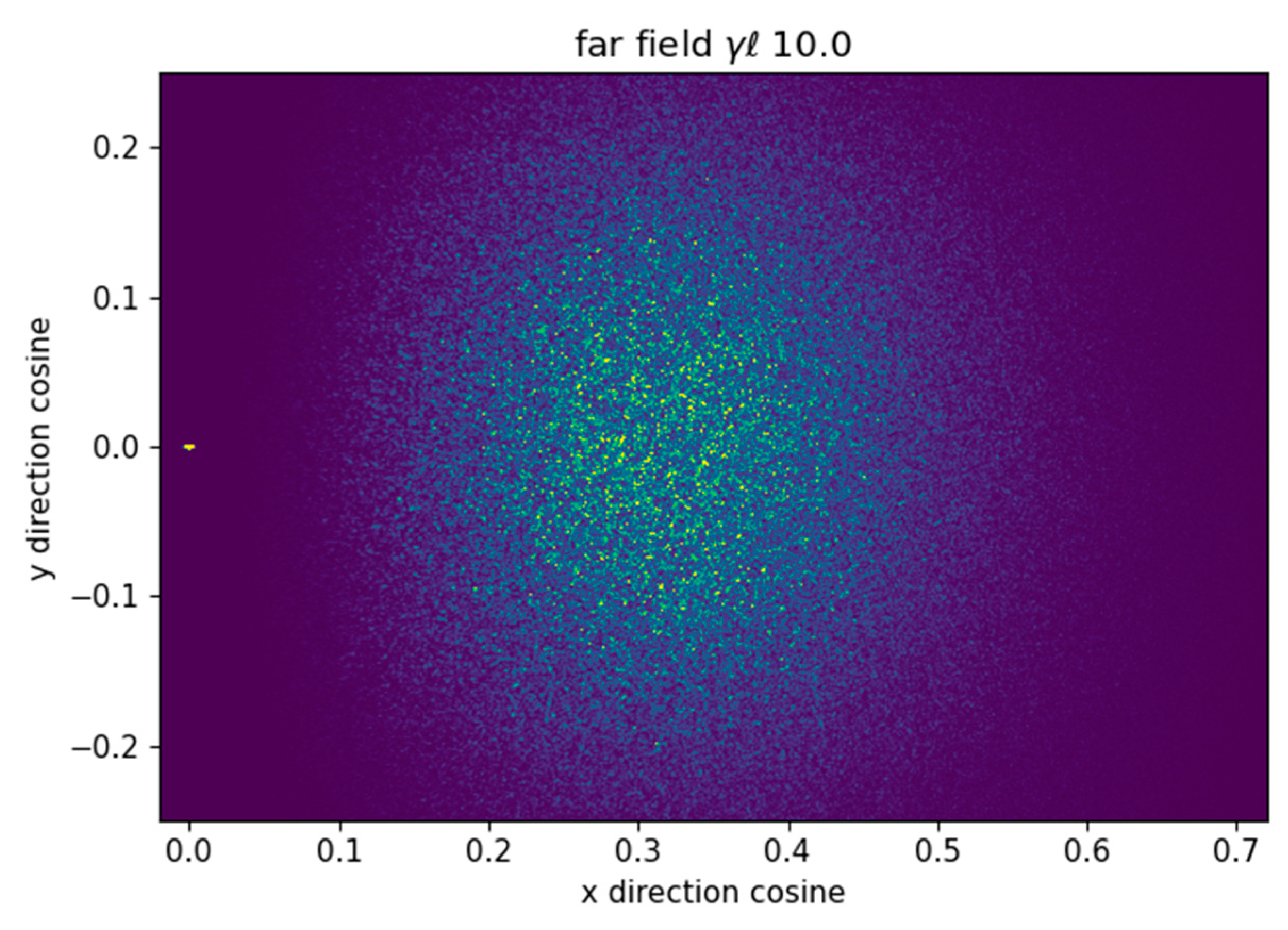
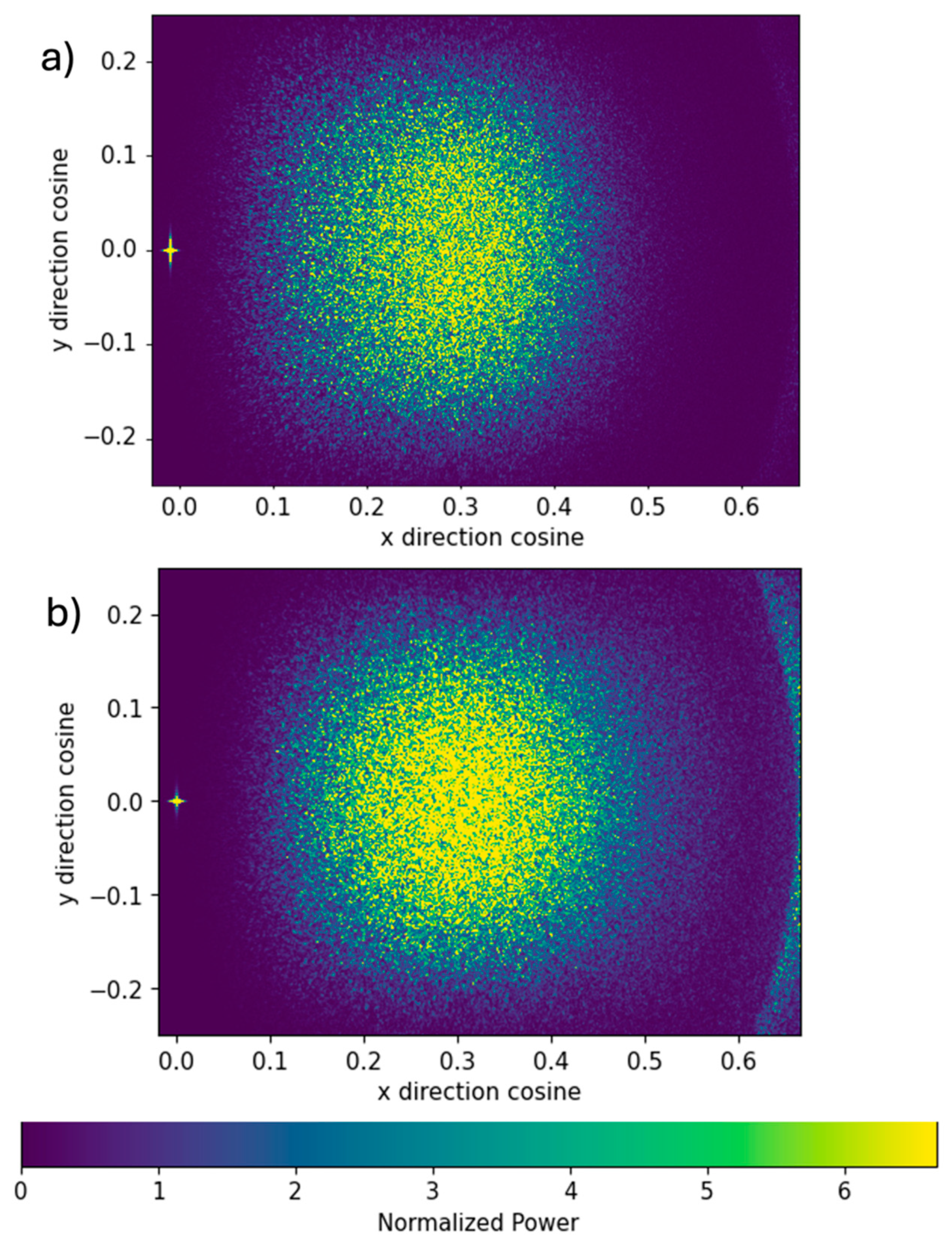
- Coupling to the longitudinal grating formed by the equally spaced nonlinear transparencies. This feature is especially apparent in models of the fanning effect, in that it results in the appearance of rings centered on the direction of the incident beams in the far field where the fanning pattern is usually observed. The diameter of these rings is approximately proportional to the inverse of the square root of the step size. Step sizes less than 5mm will usually push the diameter of the innermost ring beyond the region of interest in the far field.
- Wraparound effects due to the intrinsic periodic nature of the discrete Fourier transform. This last effect could be controlled by using finite difference beam propagation methods instead of FFT methods, but this would unnecessarily introduce additional complexity. We have chosen to continue to use FFT methods with the understanding that wraparound effects need to be acknowledged and minimized by choosing transverse apertures large enough to keep the main parts of the interacting beams away from the boundaries. We will see below that the periodic nature of the FFT is advantageous when seeking to verify the code against standard plane wave theory.
2. Methods
- The vector angular spectrum of plane waves method requires separate handling of the ordinary and extraordinary vector modes which are both dependent on the transverse spatial frequencies[20].
- Use of the full electro-optic tensor would require knowledge of the longitudinal components of the photorefractive space charge field which depend on the three-dimensional gradient of the optical intensity . The methods used in the past, and in this paper ignore the longitudinal component of the intensity gradient and space charge electric field: the grating is calculated assuming that it is independent of the optical fields at neighboring planes.
- Nevertheless, the scalar quasi-3D method described below does match many experimental results.
2.1. Beam Propagation
2.2. Photorefractive Nonlinearity Model
3. Results
3.1. Two-Beam Coupling
3.2. Image Amplification
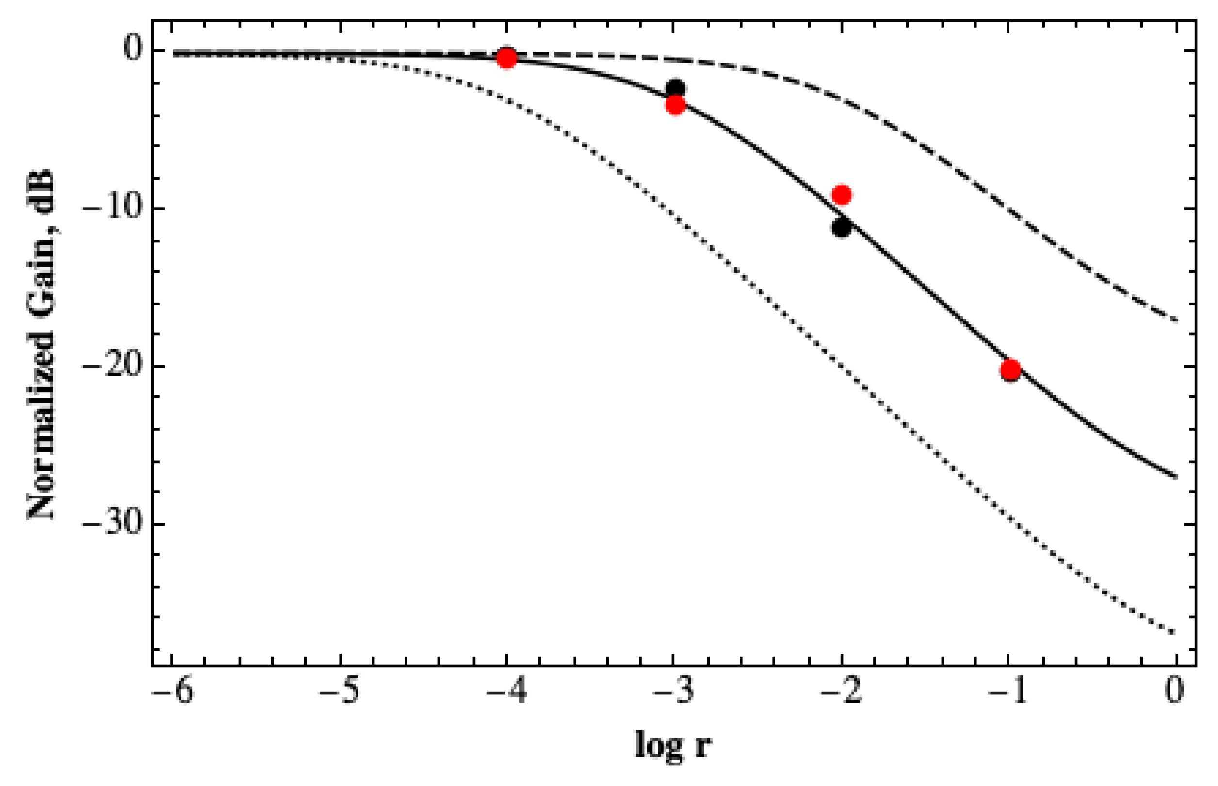
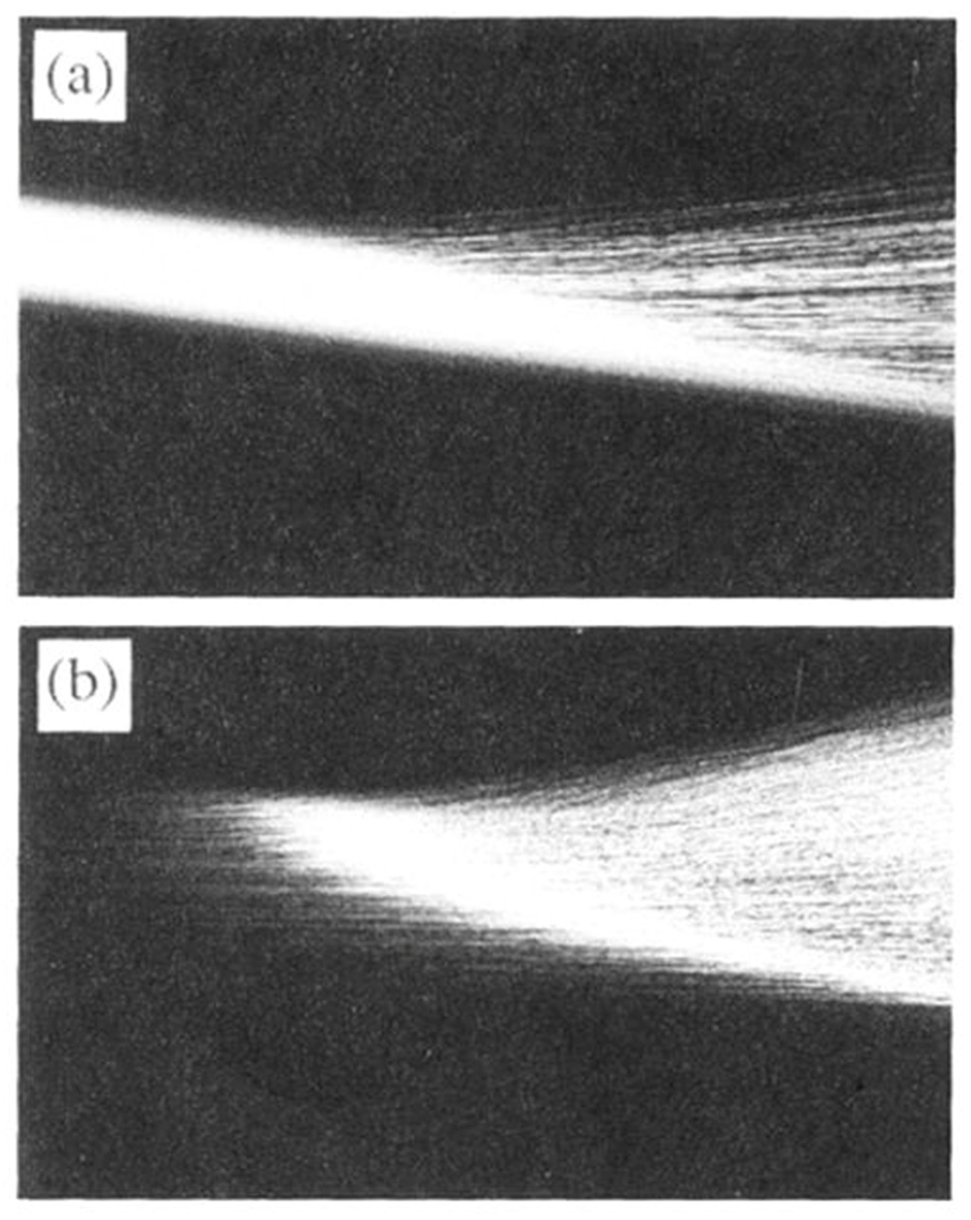
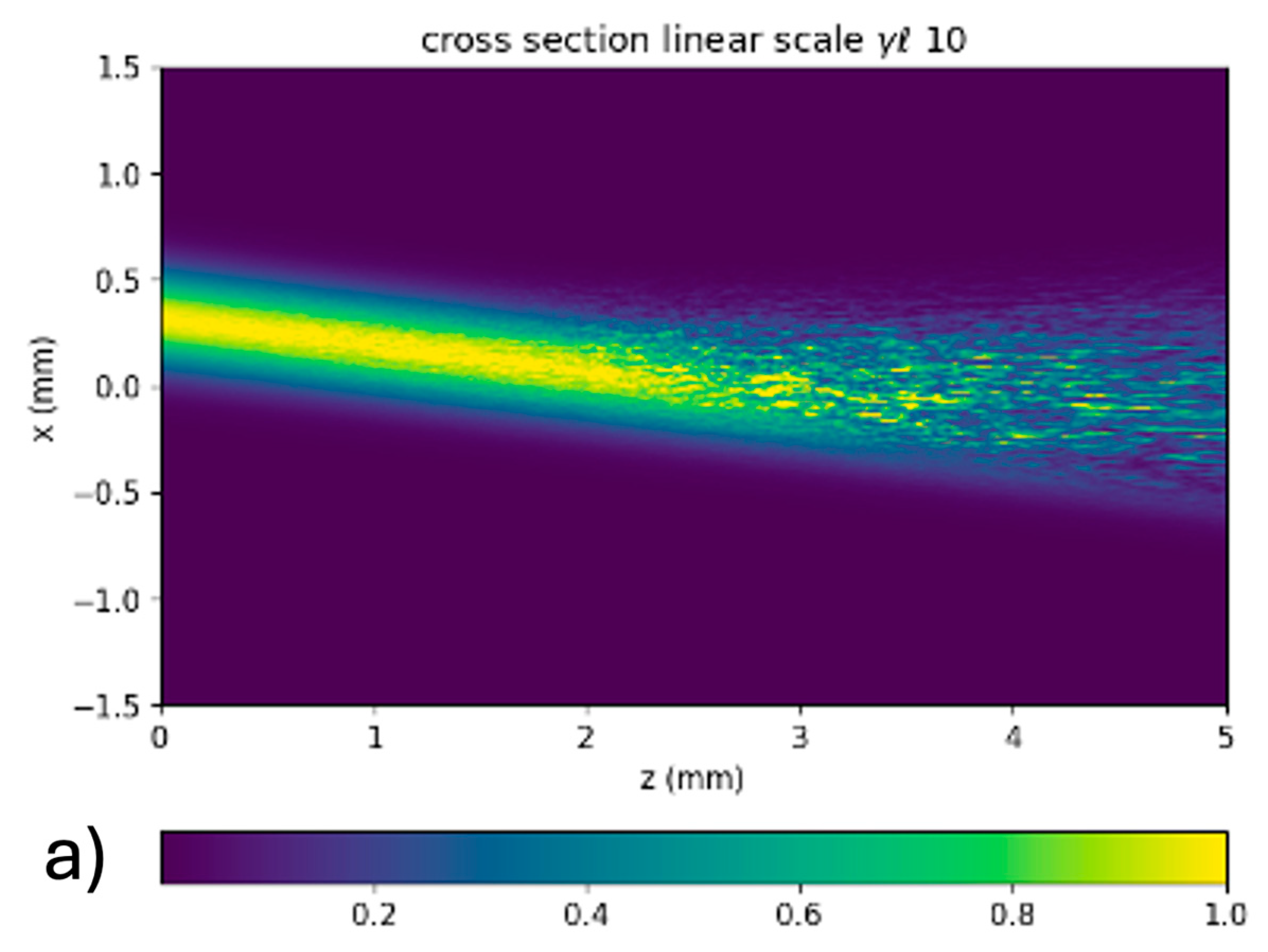
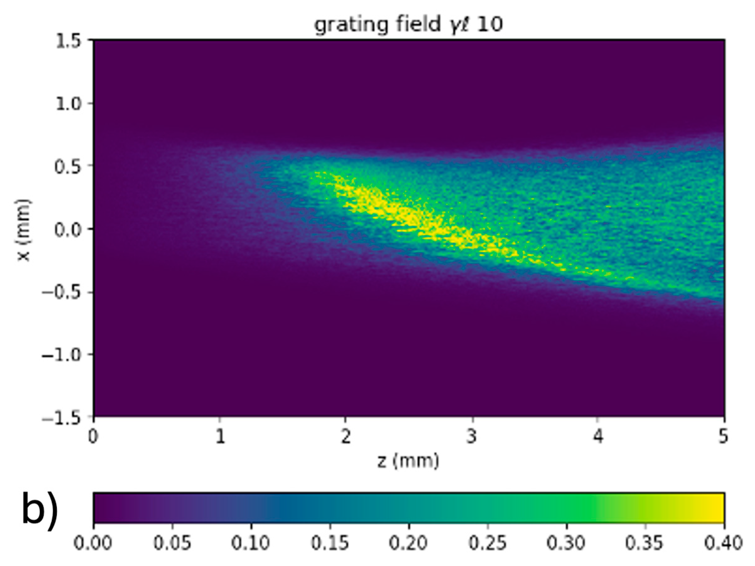
3.3. Photorefractive Amplified Scattering
3.4. Time Dependence
3.5. Time Dependent Amplified Scattering
4. Discussion
- Validity of the method and its computational limitations. Many of the prior results concentrated on analyzing the fields within the crystal, not the far field output. It is in the far field that deficiencies of the model are most apparent through the appearance of scattering ring computational artifacts. In this paper we have given some guidelines for the mitigation of these artifacts, mainly by the judicious choice of propagation step sizes.
- Extension of the scalar model from two to three dimensions. This has been enabled by improvements in available computational power since the 1990’s, in terms of data storage, random access memory, the availability of multicore processors and GPUs for parallel processing.
- Extension of the model from scalar to vector fields and the ability to model propagation in birefringent crystals considering the full electrooptic tensor.
- Inclusion of thermal effects. These become important when the intensity of the beams becomes so large that temperature dependent refractive index changes important. This effect can be significant since many photorefractive crystals are ferroelectric crystals near their Curie temperatures.
5. Conclusions
Supplementary Materials
Funding
Data Availability Statement
Conflicts of Interest
Appendix A. Program Description
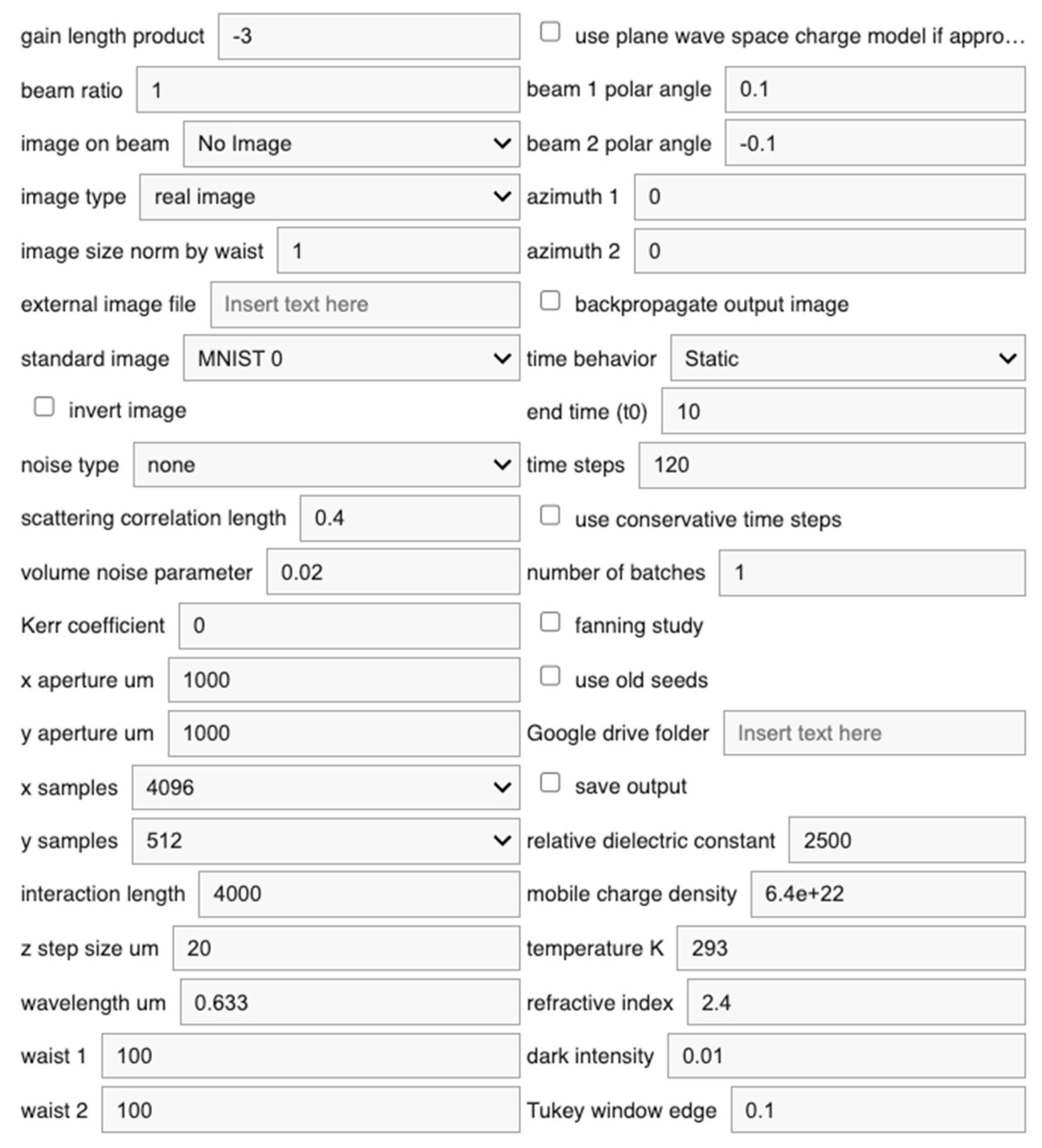
- gain length product: The standard interaction strength used in the plane wave photorefractive theory. It is the length of the interaction region times the coupling constant γ corresponding to the case where the grating wavenumber kg equals the characteristic wavenumber k0.
- beam ratio: The ratio of the peak intensity of beam 2 to beam 1. This corresponds to the parameter r in the plane wave theory. While this paper is written in terms of beam 2 being the signal and beam 1 the pump, it is beam 1 which is most closely monitored in the program. Amplification of beam 1 requires that the gain be set negative.
- image on beam: A dropdown to specify whether an image is to be applied at the input to one or both beams. This is useful for examining the nonlinearity induced image distortions.
- image type: Determines whether the image is applied as an amplitude or phase transparency.
- image size normalized by waist: The ratio between the transverse extent of the image to the waist of beam 1.
- external image file: The path in a Google drive to a user supplied image for application the input. If there is no file at the path specified, the image specified in the standard image dropdown will be used if called for.
- standard image: This dropdown is used to specify which of eleven standard supplied images will be used. One example of an MNIST digit for each of the digits 0 through 9 is supplied, as well as a 1951 Air Force Resolution Chart.
- invert image: A toggle to provide the option to invert the gray scale of the input image. This is sometimes useful for avoiding sharp edges at the image boundary.
- noise type:
- scattering correlation length: The correlation length (μm) of the Gaussian random phase screens used to model optical scattering in the crystal.
- volume noise parameter: scattering amplitude parameter ε: Number of scattering phase screens times mean square deviation of each phase screen.
- Kerr coefficient: magnitude of any nonlinearity that is directly proportional to the local intensity such as those due to thermal effects.
- x aperture um: The transverse extent in micrometers of the interaction region in the x direction.
- y aperture um: The transverse extent in micrometers of the interaction region in the y direction.
- x samples: Number of grid points in the x direction.
- y samples: Number of grid points in the y direction.
- interaction length: Length in micrometers of interaction region in z direction. Normally, the propagation axes of the two beams, beam 1 and beam 2 will be in the xz plane (azimuth zero, see below).
- z step um: The longitudinal step size in micrometers. Proper modelling of the optical effects of fine (micrometer scale) refractive index variations often requires step sizes of 10μm or less.
- wavelength um: Optical wavelength in free space in micrometers.
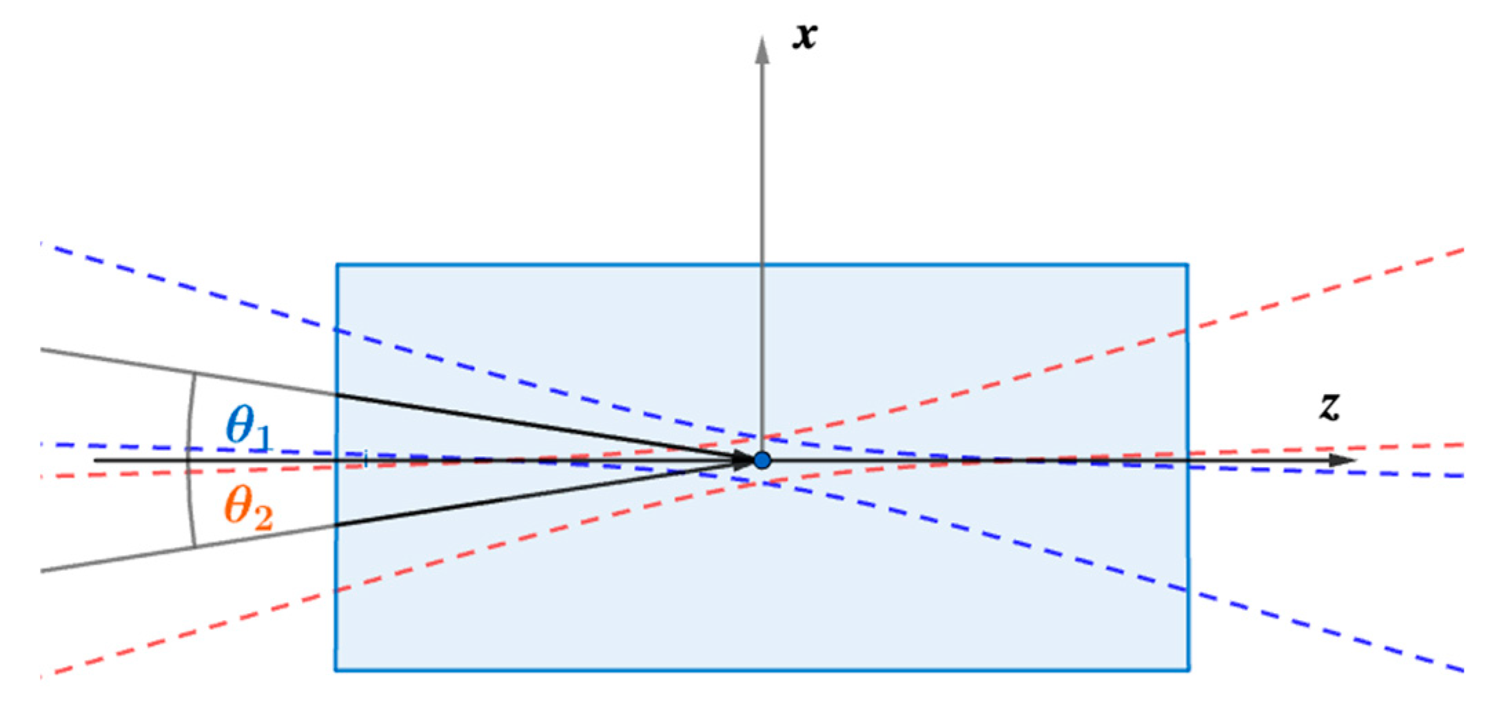
- waist 1: The input beams are generated using the standard gaussian beam formula. The waist of beam 1 at its focus is waist 1. Its focus is halfway along the interaction length. If the beam waist is entered as a negative number, plane wave incidence is assumed, This can be used for cross checking results with the standard plane wave two beam coupling theory[24]. If checked, the beam incidence angles will be set symmetrically to the wraparound effect free angles closest to the one initially specified in the beam 1 polar angle field. See Equation (8).
- waist 2: The waist of beam 2.
- use plane wave space charge model if appropriate: For use when using plane wave two beam coupling theory. Only available for two coupled plane waves propagating in xz plane with symmetric incidence angles.
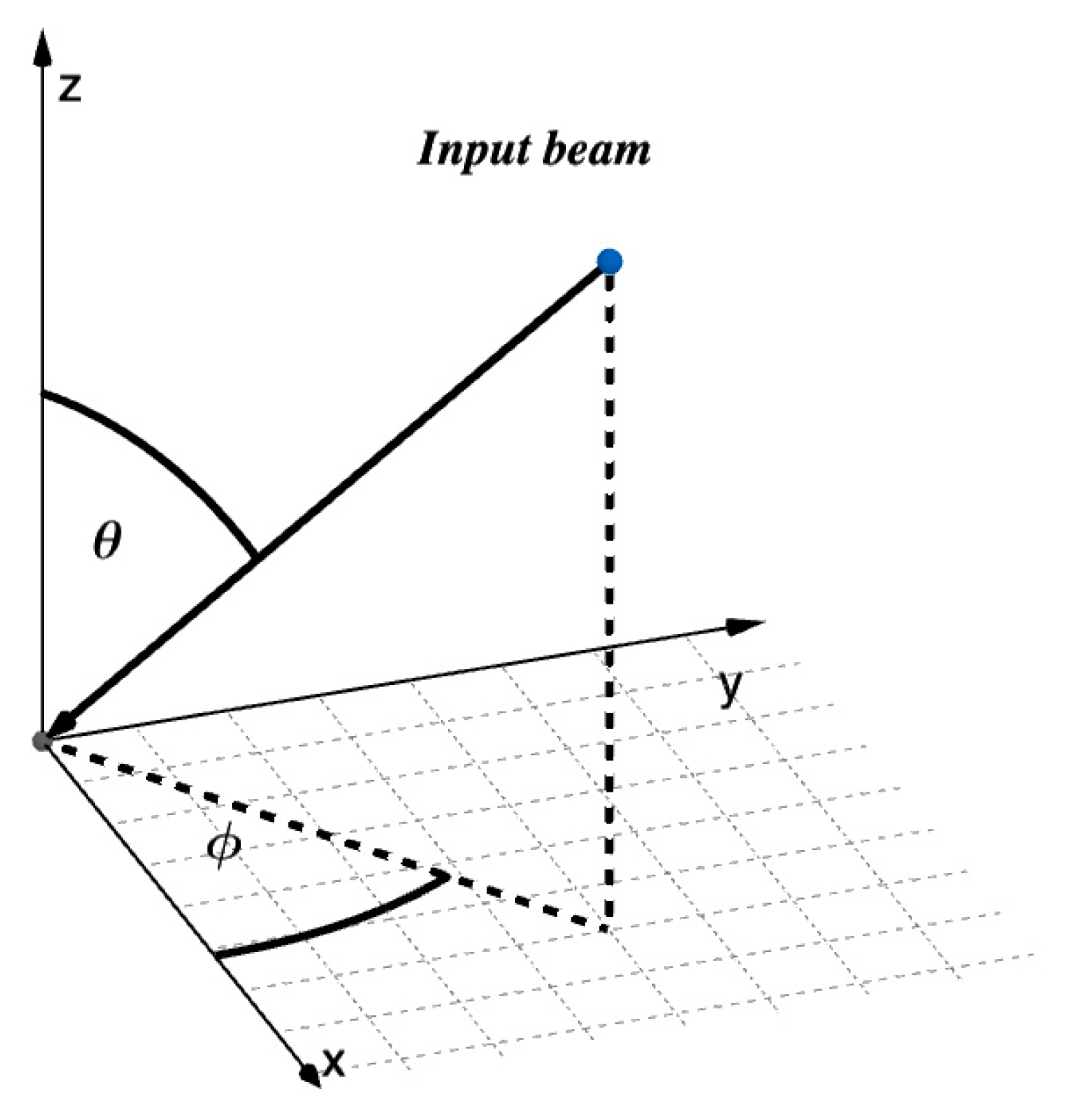
- beam 1 polar angle: The polar angle of incidence of beam 1,. The definition of the angles is shown in Figure A3.
- beam 2 polar angle: The polar angle of incidence of beam 2,
- azimuth 1: The azimuth of beam 1,
- azimuth 2: The azimuth of beam 1,
- backpropagate output image: This gives the option to backpropagate the output field in beam 1 to the input plane without nonlinearities to allow comparison of images before and after photorefractive image processing, for example amplification. Without backpropagation, regular diffractive effects appear which can obscure distortions due to the photorefractive effect. Backpropagation is equivalent to bringing the output to an image plane.
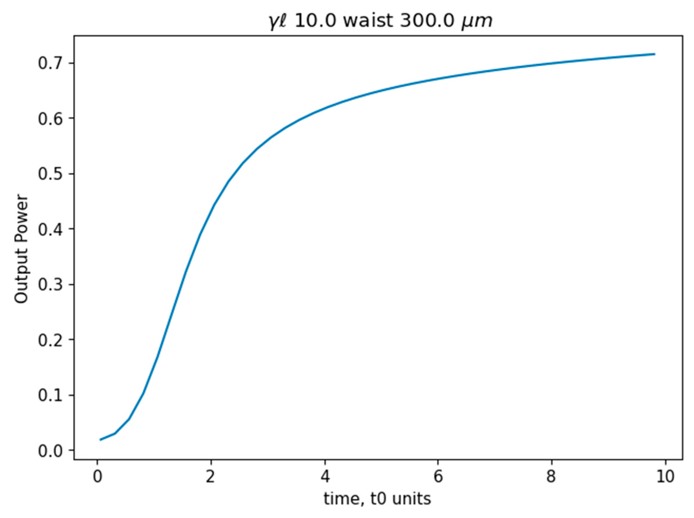
- time behavior: Choosing “Static” invokes the time independent model where the partial derivatives with respect to time are set to zero. Choosing “Time Dependent” invokes the full time dependent model and generates movies showing time dependence and a graph of the power in beam 1 as a function of time as it is amplified or deamplified via two beam coupling. Time dependent calculations place a significant load on memory, since the full three-dimensional space charge electric field must be stored from one time step to the next.
- end-time: The duration of the simulation in units of the characteristic time t0 (see appendix B). One time step equals the end-time/number of time steps.
- time steps: the number of time steps taken by the model before completion.
- use conservative time steps: Set the time step to one fourth of the minimum anticipated time constant, 1/(1+(kg/k0)2)
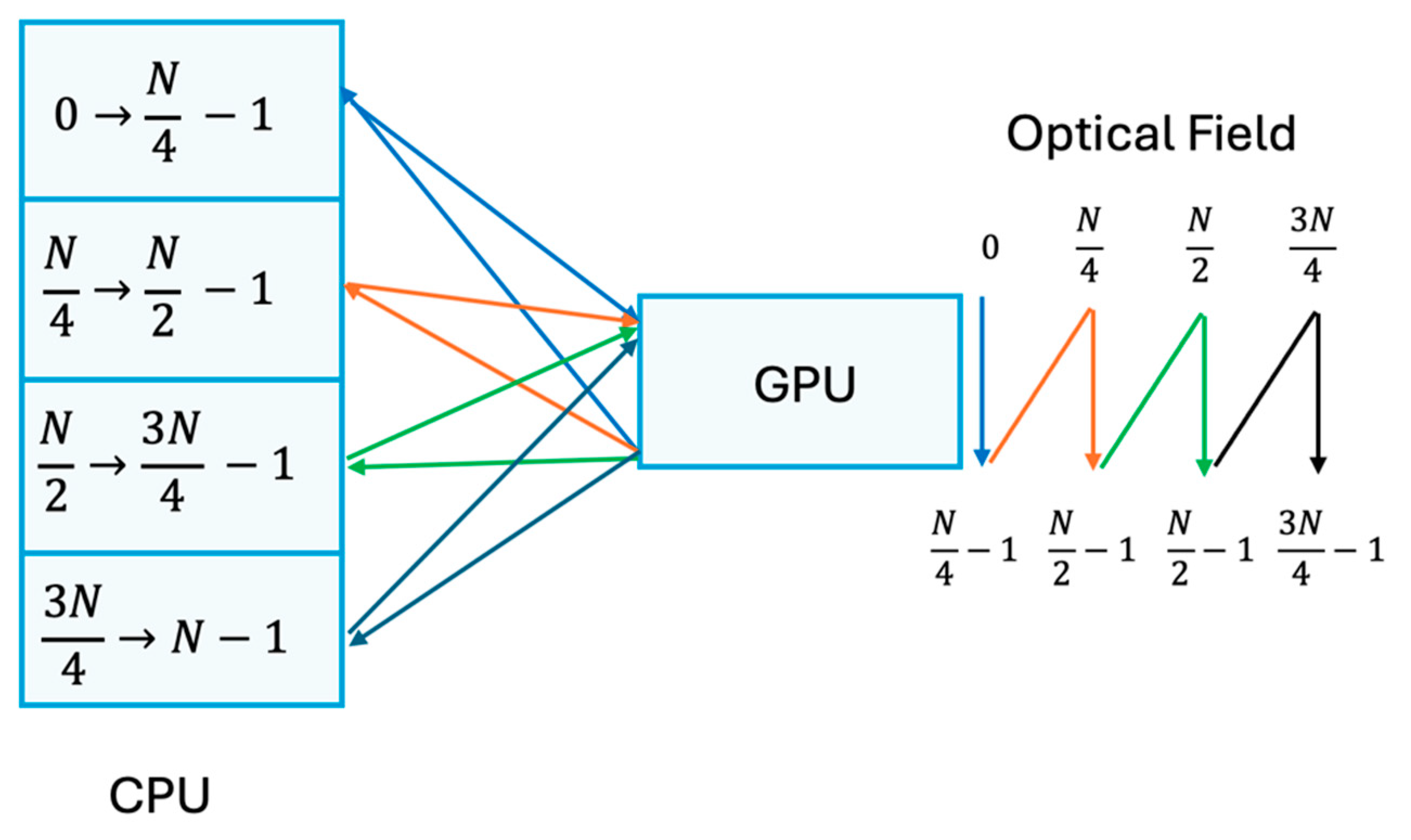
- number of batches: The propagation can be split into several longitudinal batches so that the GPU only needs to store the part of the space charge fields required by the current batch. The full three-dimensional space charge field is stored in the CPU. On Google COLAB’s A100 there are 83.5 GB CPU RAM available and 40 GB GPU RAM.
- fanning study: If selected, spatial frequencies corresponding to the input beam are masked out in the far field so that the amplified scattering can be displayed without saturation by the remnants of the input beam.
- use old seeds: Use noise seeds already stored in the prdata dictionary for the current calculation. For example, if comparing static and time dependent fanning distributions. The static case might be run first, its noise seeds saved the dictionary, then reused for a time dependent calculation. If the seeds dictionary is empty, new noise seeds will be generated. The seeds for each run are stored in the run’s dictionary (prdata).
- Google drive save folder: When save output is selected, contains the name of the folder on Google Drive where run parameters in the prdata dictionary (saved in the file data.json), output images and movies (for time dependent runs) are stored. If the folder does not exist it will be created.
- save output: If selected the run’s data will be stored to disk. It can be retrieved at the beginning of each run instance.
- relative dielectric constant: The dielectric constant of the interaction crystal normalized by the permittivity of free space .
- temperature K: Temperature in Kelvin.
- refractive index: Crystal refractive index. Default is a typical refractive index for BaTiO3 (data available from various sources)
- dark intensity: Equivalent optical intensity accounting for thermally ionized carriers. This intensity accounts for dark decay of the gratings. Normalized to the sum of the average peak intensity I0 of the beams. (See appendix B)
- Tukey window edge: The edge parameter for the Tukey (cosine taper) window[31] used to enable absorbing boundaries of the propagation lattice in both real space and Fourier space
Generation of input field
Appendix B. The Photorefractive Model
Appendix C. Artifacts
Limitations on Step Size
High Order Diffraction
Wraparound Artifacts Due to the Periodic Nature of the Discrete Fourier Transform Space
References
- Aisawa, S.; Noguchi, K.; Matsumoto, T. Remote Image Classification through Multimode Optical Fiber Using a Neural Network. Optics Letters 1991, 16, 645-647.
- Ancora, D.; Negri, M.; Gianfrate, A.; Trypogeorgos, D.; Dominici, L.; Sanvitto, D.; Ricci-Tersenghi, F.; Leuzzi, L. Low-power multimode-fiber projector outperforms shallow-neural-network. Physical Review Applied 2024, 21. [CrossRef]
- Dudley, J.; Genty, G.; Coen, S. Supercontinuum generation in photonic crystal fiber. Reviews of Modern Physics 2006, 78, 1135-1184. [CrossRef]
- Tegin, U.; Yildirim, M.; Oguz, I.; Moser, C.; Psaltis, D. Scalable optical learning operator. Nature Computational Science 2021, 1, 542-549. [CrossRef]
- Gunter, P.; Huignard, J.P. Photorefractive Materials and Their Applications 1: Basic Effects; Springer: New York, 2005; p. 426.
- Segev, M.; Engin, D.; Yariv, A.; Valley, G.C. Temporal Evolution of Fanning in Photorefractive Materials. Optics Letters 1993, 18, 956-958. [CrossRef]
- Skeldon, M.; Narum, P.; Boyd, R. Non-Frequency-Shifted, High-Fidelity Phase Conjugation with Aberrated Pump Waves by Brillouin-Enhanced 4-Wave-Mixing. Optics Letters 1987, 12, 343-345.
- Lind, R.; Steel, D. Demonstration of the Longitudinal Modes and Aberration-Correction Properties of a Continuous-Wave Dye Laser with a Phase-Conjugate Mirror. Optics Letters 1981, 6, 554-556.
- Feinberg, J.; Hellwarth, R.W. Phase-Conjugating Mirror with Continuous-Wave Gain. Optics Letters 1980, 5, 519-521. [CrossRef]
- White, J.O.; Croningolomb, M.; Fischer, B.; Yariv, A. Coherent Oscillation by Self-Induced Gratings in the Photorefractive Crystal BaTiO3. Applied Physics Letters 1982, 40, 450-452.
- Feinberg, J. Self-Pumped, Continuous-Wave Phase Conjugator Using Internal-Reflection. Optics Letters 1982, 7, 486-488. [CrossRef]
- Cronin-Golomb, M. Whole Beam Method for Photorefractive Nonlinear Optics. Optics Communications 1992, 89, 276-282. [CrossRef]
- Zozulya, A.A.; Saffman, M.; Anderson, D.Z. Propagation of Light-Beams in Photorefractive Media - Fanning, Self-Bending, and Formation of Self-Pumped 4-Wave-Mixing Phase-Conjugation Geometries. Physical Review Letters 1994, 73, 818-821. [CrossRef]
- Brown, W.P.; Valley, G.C. Kinky Beam Paths Inside Photorefractive Crystals. Journal of the Optical Society of America B-Optical Physics 1993, 10, 1901-1906. [CrossRef]
- Ratnam, K.; Banerjee, P.P. Nonlinear Theory of 2-Beam Coupling in a Photorefractive Material. Optics Communications 1994, 107, 522-530. [CrossRef]
- Fainman, Y.; Klancnik, E.; Lee, S.H. Optimal Coherent Image Amplification by 2-Wave Coupling in Photorefractive BaTiO3. Optical Engineering 1986, 25, 228-234. [CrossRef]
- Zozulya, A.A.; Anderson, D.Z. Spatial Structure of Light and a Nonlinear Refractive-Index Generated by Fanning in Photorefractive Media. Physical Review A 1995, 52, 878-881. [CrossRef]
- Horowitz, M.; Kligler, D.; Fischer, B. Time-Dependent Behavior of Photorefractive 2-Wave and 4-Wave-Mixing. Journal of the Optical Society of America B-Optical Physics 1991, 8, 2204-2217. [CrossRef]
- Goodman, J.W. Introduction to Fourier optics, Fourth edition. ed.; W.H. Freeman, Macmillan Learning: New York, 2017; pp. xiv, 546 pages.
- Muys, P. Propagation of vectorial laser beams. Journal of the Optical Society of America B-Optical Physics 2012, 29, 990-996.
- Feinberg, J.; Heiman, D.; Tanguay, A.R.; Hellwarth, R.W. Photorefractive Effects and Light-Induced Charge Migration in Barium-Titanate. Journal of Applied Physics 1980, 51, 1297-1305.
- Vahey, D.W. Nonlinear Coupled-Wave Theory of Holographic Storage in Ferroelectric Materials. Journal of Applied Physics 1975, 46, 3510-3515. [CrossRef]
- Cronin-Golomb, M.; Fischer, B.; White, J.; Yariv, A. Theory and Applications of 4-Wave Mixing in Photorefractive Media. IEEE Journal of Quantum Electronics 1984, 20, 12-30. [CrossRef]
- Kukhtarev, N.V.; Markov, V.B.; Odulov, S.G.; Soskin, M.S.; Vinetskii, V.L. Holographic Storage in Electrooptic Crystals .1. Steady-State. Ferroelectrics 1979, 22, 949-960.
- Feinberg, J. Asymmetric Self-Defocusing of an Optical Beam from the Photorefractive Effect. Journal of the Optical Society of America 1982, 72, 46-51. [CrossRef]
- Montemezzani, G.; Zozulya, A.A.; Czaia, L.; Anderson, D.Z.; Zgonik, M.; Gunter, P. Origin of the Lobe Structure in Photorefractive Beam Fanning. Physical Review A 1995, 52, 1791-1794. [CrossRef]
- Vachss, F. An Analytic Expression for the Photorefractive Two Beam Coupling Response Time. In Proceedings of the Topical Meeting on Photorefractive Materials, Effects, and Devices II, Aussois, 1990/01/17, 1990; p. BP8.
- Iserles, A. A First Course in the Numerical Analysis of Differential Equations, Second ed.; Cambridge University Press: Cambridge, 2009.
- PARSHALL, E.; CRONIN-GOLOMB, M.; BARAKAT, R. Model of Amplified Scattering in Photorefractive Media - Comparison of Numerical Results and Experiment. Optics Letters 1995, 20, 432-434. [CrossRef]
- Garrett, M.H.; Chang, J.Y.; Jenssen, H.P.; Warde, C. High Beam-Coupling Gain and Deep-Trap and Shallow-Trap Effects in Cobalt-Doped Barium-Titanate, BaTiO3-Co. Journal of the Optical Society of America B-Optical Physics 1992, 9, 1407-1415. [CrossRef]
- Harris, F.J. Use of Windows for Harmonic-Analysis with Discrete Fourier-Transform. Proceedings of the Ieee 1978, 66, 51-83. [CrossRef]

| Parameter | Static Calculation | Dynamic Calculation |
| Coupling | 10.0 | 10.0 |
| x aperture mm | 3.0 | 1.5 |
| y aperture mm | 2.0 | 0.75 |
| Number of x samples | 16384 | 4096 |
| Number of y samples | 4096 | 2048 |
| Crystal length mm | 5.0 | 5.0 |
| Scattering corr. length mm | 0.4 | 0.4 |
| Longitudinal step size mm | 2 | 8 |
| Wavelength mm | 0.488 | 0.488 |
| Beam waist mm | 0.3 | 0.3 |
| Dark intensity | 0.01 | 0.01 |
| Angle of incidence radians | 0.3 | 0.3 |
| Azimuth of incidence rad | 0.0 | 0.0 |
| Time Steps | NA | 160 |
| End time normalized | NA | 10 |
| Tukey window parameter | 0.2 | 0.2 |
| GPU batches | 1 | 5 |
| A100 calc. time hh:mm | 0:05 | 1:57 |
| A100 CPU RAM GB | 7.2 | 71.9 |
| A100 GPU RAM GB | 31 | 38 |
Disclaimer/Publisher’s Note: The statements, opinions and data contained in all publications are solely those of the individual author(s) and contributor(s) and not of MDPI and/or the editor(s). MDPI and/or the editor(s) disclaim responsibility for any injury to people or property resulting from any ideas, methods, instructions or products referred to in the content. |
© 2025 by the authors. Licensee MDPI, Basel, Switzerland. This article is an open access article distributed under the terms and conditions of the Creative Commons Attribution (CC BY) license (http://creativecommons.org/licenses/by/4.0/).


