
Submitted:
30 December 2024
Posted:
31 December 2024
You are already at the latest version
Abstract
This study describes a sensor system for continuous monitoring of VOCs emitted from small industrial facilities in urban centers, such as automobile paint facilities and printing facilities. Previously, intermittent measurements were made using expensive FID-type instruments that were impossible to install, resulting in a lack of continuous management. This paper develops a low-cost sensor system for full-time management and consists of multi sensor systems to increase the spatial resolution in the pipe. To improve the accuracy and reliability of this system, a new RANFIS algorithm with enhanced preprocessing based on ANFIS algorithm is proposed. For this purpose, a smart sensor module consisting of low-cost MOS and PID sensors is fabricated, and an operating controller is configured for real-time data acquisition, analysis, and evaluation. In the front part of RANFIS, IQR is used to remove outliers and gradient analysis is used to detect and correct data with abnormal change rate to solve nonlinearities and outliers in sensor data. At the latter stage, the complex nonlinear relationship of the data was modeled with ANFIS to reliably handle data uncertainty and noise. For practical verification, a toluene evaporation chamber with a sensor system for monitoring was built, and the results of real-time data sensing after training based on real data were compared and evaluated. As a result of applying the RANFIS algorithm, the RMSE of MQ135, MQ138, and PID-A15 sensors was 3.578, 11.594, and 4.837, respectively, which improved the performance by 87.1%, 25.9%, and 35.8% compared to the existing ANFIS. Therefore, the precision within 5% of the measurement results of the two experimentally verified sensors shows that the proposed RANFIS-based sensor system can be sufficiently applied in the field.
Keywords:
multi-sensor system
; ANFIS
; RANFIS
; learning algorithm
; low-cost sensing system
; VOCs
1. Introduction
With the development of industry and transportation, air pollutants such as O3 and particulate matter have become a serious environmental concern [1,2]. These pollutants not only adversely affect ecosystems and the environment, but also have a negative impact on human health. In particular, volatile organic compounds (VOCs) are a group of 37 air pollutants designated by the Ministry of the Environment for control, including health hazards such as acetaldehyde and formaldehyde, as well as ozone precursors such as benzene, toluene, and xylene. VOCs measurement is used in a variety of applications, including indoor air quality, fire detection, odor monitoring, and factory emissions [3]. Industrial facilities, such as automotive paint facilities, are one of the major sources of VOCs emissions, and it is necessary to accurately measure VOCs emissions from these facilities [4,5].
To accurately measure VOCs, flame ionization detectors (FIDs) are commonly used as the recognized VOCs detector. Although FIDs provide high accuracy and a wide measurement range, they are difficult to install in factories at all times due to the high cost of the equipment, and periodic measurements are also costly, so they rely on rental or door-to-door measurements. Therefore, to solve these problems, a full-time self-measurement system utilizing low-cost gas sensor such as photo ionization detectors (PIDs) and metal oxide semiconductors (MOSs) systems can be considered as an alternative.
PID sensors are characterized by high sensitivity and relatively low cost, and MOS sensors are attracting attention for their affordability and reasonable lifetime [6,7]. However, low-cost gas sensors have limitations such as unstable measurement accuracy due to initialization, environmental factors such as temperature and humidity, and nonlinear data due to sensor aging [8,9,10]. In addition, the feature of gas materials makes it difficult to measure at a precise location, so measurements are made at a specific location [11]. However, when composed of low-cost sensors, it is difficult to trust a single measurement.
To improve this, researchers have been utilizing multi-sensor and AI algorithms. Previous studies have constructed sensor arrays with various MOS sensors and used neural networks (BPNN-DT) or PLS models to predict VOCs concentrations [12,13], but these approaches were mainly performed in a confined laboratory environment, which limits their applicability in real factory environments. MLR and ANN models have been used in studies to calibrate accurate data in complex environments such as factory exhaust, and ANNs in particular have the advantage of modeling nonlinear data [14,15]. However, ANN models rely on high-quality training data and can perform poorly on noisy data. Preprocessing such training data to detect and remove outliers plays an important role, and statistical analysis such as standard deviation, median absolute deviation, and interquartile range (IQR) have been widely used to determine outliers [16].
To overcome these limitations and improve the accuracy of VOCs measurement, this paper proposes a multi-sensor system based on the Reinforced Adaptive Neuro Fuzzy Inference System (RANFIS). The system uses multi sensors system to improve the spatial resolution in gas exhaust vents and reliably calibrates sensor data using the RANFIS algorithm, which combines fuzzy logic and reinforcement learning. The algorithm effectively handles nonlinear multi-sensor data, analyzes outliers to detect sensor anomalies, and corrects for noise in the data. This improves the accuracy of VOCs measurement and enables a system that can systematically manage VOCs emissions in a factory around the clock. The RANFIS-based sensor system is an economical and efficient alternative to expensive equipment and is expected to contribute to real-time VOCs monitoring in industrial sites.
2. Multi Sensor Module and Experimental
2.1. Low-Cost Multi Sensor Module and Reference Sensor
FIDs provide high accuracy, but FIDs such as the phx42 [17], which is often used as a certified measurement, are expensive equipment, making full-time measurement prohibitive for operators of small urban VOCs emitters. As an alternative, measurements utilizing relatively inexpensive PIDs and MOS sensors have been proposed as an alternative, but their low precision affects the reliability of the measurements. In this study, a unit multi-sensor module including three low-cost VOCs sensors and a temperature and humidity sensor was fabricated for VOCs emission measurement. Table 1 shows the low-cost VOCs sensors included in the multi-sensor module and the REF sensor for precise measurements. The MOS sensor measures the change in electrical resistance in response to VOCs, and the PID sensor uses a UV light source to ionize gas molecules to measure their concentration. The sensors used to build the unit multi-sensor module are MQ135 (0-1000 ppm) [18], MQ138 (0-500 ppm) [19], and PID-A15 (0-4000 ppm, 100 ppb resolution) [20], and a high-end PID meter FIX800 [21] was built to measure environmental data.
2.2. Data Measurement and Analysis
As shown in Figure 1a, the multi-sensor module is designed to operate based on the CORTEX-M3 MCU, with the sensors on the top of the PCB and the power and communication components inside the case. The multi-sensor module is connected to the control PC via CAN communication and is configured to allow real-time data transmission and reception between multi sensor system. The Host MCU sends CAN messages, the Client MCU receives and processes the sensor data and sends it to the control PC, and the data is stored in the DB.
The exhaust of automotive paint facilities, which are small VOC emitters in urban centers, are essentially equipped to prevent VOC emissions. The airflow in the vent of this facility varies depending on the installation location, shape, internal wind speed, and particle size in the vent [22,23,24], which makes it difficult for sensors to perform stable and accurate measurements. Therefore, in this study, we aim to improve the accuracy of the measurement by placing multi sensor system inside the exhaust vent to increase the spatial resolution. For this purpose, a multi-sensor system as shown in Figure 1 for VOCs measurement was constructed to obtain data and validate the proposed method in a real environment. Figure 1b shows the structure of the developed unit multi-sensor module, and Figure 1c shows the configuration of the multi-sensor system consisting of eight sensor modules actually installed.
The emission prevention facility at the workplace consists of a HEPA filter and an activated carbon filter, and the wind speed and pressure decrease at the exhaust after the activated carbon filter. In previous related studies on activated carbon filters and fine dust filters, the experimental chamber was designed to reflect this [25,26]. Since this study also measures VOCs by attaching a sensor module to the rear end of the activated carbon filter, a chamber for evaluating multi-sensor systems and algorithms for monitoring systems in a testbed environment before actual field verification was constructed as shown in Figure 2. POS 1-8 in Figure 2 show the locations of the sensor modules attached to the designed chamber.
2.3. Testbed Setup
The testbed was constructed to allow the introduction of zero gas and VOCs into the chamber. High-purity nitrogen (N2, 99.9%) was used as the zero gas, and toluene was used as the VOC input gas. Toluene is one of the most common VOCs emitted from automotive paint facilities, along with butyl acetate and xylene [4].
Figure 3a shows the conceptual diagram of the experiment, and Figure 3b shows the actual built testbed experimental environment. The gas flow control was performed using a Mass Flow Controller (MFC) from Bronkhorst, with a maximum flow rate of 215 ml/min. The MFC precisely controls the flow rate of the incoming zero gas, allowing the air velocity and pressure inside the chamber to be adjusted. To relieve the pressure at the point where the zero gas meets the VOCs, a bypass was designed in the mixing path of the two gases with a check valve connection to prevent excessive pressure.
In the experiments, toluene in liquid form as a VOC input was placed in a 60 ml syringe and injected precisely via a syringe pump. The injected toluene is vaporized and used in the experiment before entering the chamber. A total of eight multi-sensor modules were attached to the inside of the chamber, and the multi-sensor system measured VOCs concentrations at 2s intervals. At the end of the chamber, a reference sensor called FIX800 was installed to verify and calibrate the VOCs concentration. This testbed-based experimental environment was operated to precisely measure the concentration changes of VOCs and analyze the response characteristics of the sensor.
The data acquired from the sensor modules is efficiently managed through a Python-based data collection and processing program. The VOCs data measured by the multi-sensor system is stored in MariaDB in real time to ensure data stability and security. The dataset was generated by setting the VOCs measurement data of the sensor module as the input and the VOCs data measured by the reference sensor as the answer value. The experiments were conducted twice for 8 hours and 7 hours, respectively, and a total of 14631 and 12629 data points were obtained. The first experiment was utilized to train the algorithm based on the sensor data, while the second experiment was configured separately to evaluate the performance of the trained model.
2.4. Data Charateristics
A normalized comparison of the VOCs measurement data from each multi-sensor module within the chamber revealed that the measurements varied depending on the sensor position attached to the chamber. As shown in Figure 4, the graph plots for Position 1 and 5 of Sensor 1 attached to the top of the chamber were similar, while the graph plots for Position 4 and 8 attached to the right side of the chamber were similar to each other. This clearly shows the difference in sensor response depending on the attachment position in the chamber and indicates the need for a detailed evaluation of the position. Figure 5 and Figure 6 provide a comparison of the normalized graphs of Sensor 2 and Sensor 3, respectively, but the differences are not as pronounced as for Sensor 1.
Figure 7 shows the measured and initial values for Sensors 1, 2, and 3, and Table 2, Table 3, and Table 4 show the correlation coefficients with the reference sensor for each location and the initial values of the experiment. In particular, for Sensor 1, the correlation coefficient of the sensors attached to the top and right side is relatively low, while the correlation coefficient of the sensors attached to the bottom and left side is high. In the case of the bottom and left sensors, the graph shape follows the data of the reference sensor (FIX800) well. However, when comparing the initial values before normalization, it is confirmed that there are offset differences between each sensor value even though the graph shape is similar.
The results of this analysis show that even the same type of sensor can produce different measured values depending on where it is attached, due to differences in the sensor’s own characteristics and the non-homogeneous gas concentration in the pipe. Therefore, precise calibration that takes into account the offset and location characteristics of each sensor is necessary to improve the accuracy of the measured values. However, due to the feature of gas measurement, precise calibration of multiple sensors individually is not economically feasible and time-consuming. Even if it were possible, it is almost impossible to expect reliable and accurate measurements in in-pipe measurements, where it is difficult to guarantee that the calibrated and tuned sensor modules are identical in one or two specific cases [22,23,24]. To overcome these issues, other calibration and judgment methods, such as suitable AI algorithms, are needed.
3. ANFIS Model
3.1. ANFIS Structure and Modeling
A fuzzy inference system (FIS) is a system that processes uncertain or ambiguous data and supports decision-making based on fuzzy logic. Unlike binary logic, fuzzy logic allows for intermediate states between “true” and “false,” giving a numerical representation of ambiguous human language. This allows for the analysis and control of complex nonlinear systems.
Adaptive Neuro-Fuzzy Inference System (ANFIS), proposed by JANG, is a hybrid system that combines neural networks and fuzzy inference systems to perform data-driven learning and rule-based modeling simultaneously [27]. Figure 8 shows the structure of ANFIS, which is suitable for solving complex nonlinear problems and is widely used in prediction, classification, control systems, etc.
The ANFIS model consists of five layers. Use Equation 1 to calculate the membership value of a linguistic label from the Membership Function in Layer 1.
where x is an explicit input, μ is a linguistic label, and is a membership function inside a linguistic label, and we use the usual bell-shaped formula. , and determines the shape of the Membership Function with the premise parameters. Using Equation 2, Layer 2 calculates the impact of the rule by multiplying the membership values of each Membership Function.
Layer 3 uses Equation 3 to normalize the influence to calculate the weight when generating the output.
At Layer 4, calculate the impact of each rule using Equation 4 to quantify the impact of the rule on the output.
where and are the consequent parameters to calculate the contribution of each rule. Using Equation 5, Layer 5 sums the contributions to calculate the output.
We trained an ANFIS model to model a nonlinear system using measurement data from a multi sensor system. Separate datasets were created for Sensors 1, 2, and 3, and the FIX800, an expensive PID, was set to the correct value. In the preprocessing step, an IIR filter of order 5 and cutoff frequency of 1 was applied to all datasets using Equation 6, normalized by Min-Max Scaling, and used with sensor modules at different locations. For data learning, the shape of the membership function is Gaussian bell-shaped and the epoch is set to 100.
where x[n] is the current input signal and y[n] is the current output signal, , are the feedback, feedforward coefficients, and M, N are the order of the coefficients.
First, we trained using sensor data from all locations, and in the second training, for each sensor, we excluded the sensor with the lowest correlation with the reference and trained ANFIS on the remaining seven sensors. As shown in Table 2, 3, 4, Sensor 1 had the lowest correlation of - 0.563 at Position 8, and Sensor 2 had the lowest correlation of 0.604 at Position 2. Sensor 3 had the lowest value of 0.631 at Position 6. After removing the data from these locations, we trained the ANFIS model. Finally, one common method for determining outliers is a statistical method using interquartile range (IQR) [16]. We used this method to determine the outliers in the above dataset, calibrated by replacing each outlier with the nearest normal value, and trained the ANFIS model. Figure 9 shows the train error for the above three training runs for the three sensors, and we can see that the training error decreases and converges as shown in Figure 9.
3.2. Evaluation of ANFIS Modeling
The trained models were validated for performance using RMSE and MAPE as evaluation metrics using Equations 7 and 8.
where n is the number of data, and is the raw data is the predicted data.
After training using sensor data from all locations, comparing Figure 10 with Table 5, the RMSE values are 30.406, 20.319, and 9.635 for Sensor 1, 2, and 3, respectively, with Sensor 3 performing the best. The ANFIS results excluding the sensor with the lowest correlation with the reference sensor are shown in Figure 11, and by comparing Table 5, we can see that the error is reduced compared to regular ANFIS training. These results suggest that the training dataset contains elements that interfere with learning. These elements can act as noise or outliers in the overall dataset, which not only degrade the performance of the learning model, but also disrupt the continuity of the data, causing predictions to differ significantly from the correct answer. Therefore, a method for identifying and correcting for outliers is needed.
In the above dataset, outliers are identified as shown in Figure 12, corrected by replacing each outlier with the nearest normal value, and the results of training the ANFIS model are shown in Figure 13. The RMSE of each sensor shown in Table 5 is 23.491, 12.595, and 5.703, which shows the importance of outlier correction to improve accuracy.
4. RANFIS Algorithm
4.1. RANFIS Structure
ANFIS automatically models nonlinear systems and can be precisely calibrated for each sensor. However, the dataset itself contains noise and outliers, which reduces the accuracy during training. To solve this problem, we propose the RANFIS algorithm. The RANFIS algorithm is a model that adds two layers in front of Layer 1 of the ANFIS model to analyze and remove outliers and analyze gradients to compensate for data continuity, and the RANFIS structure is shown in Figure 14.
When multiple inputs come in in real time for multi sensor system, Layer 1 uses the interquartile range (IQR) of the data coming in at a point in time to determine outliers. Use Equation 9 and Equation 10 to calculate the IQR of real-time data. And use Equation 11 to identify outliers. Using Equation 12, the data from a sensor identified as an outlier was replaced with the nearest valid value. Table 6 shows the outlier rate for each sensor. Some sensors show a high outlier rate due to sensor malfunctions, resulting in low reliability.
where x is the input data, i is the sensor location, j is the number of data in the dataset, and N is the number of sensors, is the mean of the sensor data at a point in time, and is the standard deviation. is outliers, τ is the threshold for analyzing outliers. is the sensor location excluding i.
Using Equation 13 and Equation 14, layer 2 analyzes the gradient of the incoming data at a point in time and the previous data to detect gradient analysis based outlier (GAO) of Equation 13 compared to the average of the rate of change of multi sensor system. Then the GAO’s gradient values are replaced with the nearest gradient values to correct the continuity of the data. Additionally, considering the characteristic of gas flow, the reliability of incoming sensor data is evaluated as a quality score (QS) in this work. Through GAOs, the QS is calculated based on the ratio of GAOs to cumulative data. Table 7 shows the proportion of GAO in the entire dataset. If the QS greater than or equal to R (see Equation 14) at a point in time as Sensor 1 data of Pos 5 in Table 7, the data is newly replaced with the sensor data (Sensor 1 data of Pos 3) that has the lowest QS. In this work, R is set with 40%. As shown in Figure 15, the outliers identified through gradient analysis were replaced with nearest valid gradient values.
where x is the input data, i is the sensor location, j is the number of data in the dataset, is GAO. is the data from the sensor that has the lowest QS. ∇ is the gradient of GAO with previous time point, ∇ is the gradient normal values. is the sensor location excluding i.
4.2. Results and Discussion
In Section 3, datasets were generated using Sensor 1, Sensor 2, and Sensor 3 of the 8 multi-sensor modules attached to the chamber as input data, and the FIX800 installed at the end of the chamber as the answer value. In the preprocessing step, all datasets were subjected to an IIR filter of order 5 and cutoff frequency of 1, and normalized with Min-Max Scaling to be used as input with sensor modules at different locations. As in Section 3, the same dataset was used for training and evaluation. RMSE and MAPE were used as evaluation metrics.
According to Figure 16 and Table 8, Sensor 1 is the cheapest sensor of the MOS method, and the ANFIS model results did not track the REF well and showed offset differences, with a RMSE of 29.215 and the largest prediction error. On the other hand, the RANFIS model has a RMSE of 3.758, which is 87% more accurate than ANFIS. In Figure 17 and Table 8, the RMSE of the ANIFS model on Sensor 2 is 15.654, and the RANFIS model trained on Sensor 2 is 11.594, which is a 26% improvement and more accurately tracks the shape of the REF. In Figure 18 and Table 8, for Sensor 3, both ANFIS and RANFIS models performed well, with ANFIS having a RMSE of 5.854 and RANFIS having a RMSE of 4.837, respectively, with RANFIS having a slightly lower error. As a result, it can be seen that the RANFIS model trained on data collected by 8 multi-sensor modules for VOCs measurement outperformed the ANFIS model significantly.
5. Conclusions
In this paper, we built a smart multi-sensor system with a multi-sensor module consisting of low-cost VOCs sensors and trained a RANFIS model based on the collected data to verify its potential to replace expensive VOCs sensors. The results showed that the RANFIS model outperformed ANFIS overall, especially when trained with MQ135 and PID-A15, with RMSE of 3.758 and 4.837, respectively. This proves that RANFIS is robust to nonlinear systems and robust to data containing outliers, and confirms that it is a suitable model for predicting VOCs concentrations. In particular, the prediction accuracy was maintained close to the correct value even with the low-cost MOS sensors MQ135 and MQ138, suggesting the possibility of an economical and efficient VOCs monitoring system. However, although the proposed sensor system with the RANFIS algorithm exhibits the potential to efficiently monitor VOCs through experimental verification, this study is limited to indoor experimental evaluation, which does not learn outdoor data features including various temperature and humidity changes.
As a future research, we will apply it to a real paint booth workplace to verify the performance of the RANFIS model optimized through learning by considering various environmental variables and evaluate the field applicability of the proposed sensor monitoring system.
Author Contributions
Conceptualization, K.K. and W.Y.; methodology, K.K. and W.Y.; software, K.K.; validation, K.K.; formal analysis, K.K. and W.Y.; investigation, K.K.; resources, K.K. and W.Y.; data curation, K.K.; writing—original draft preparation, K.K.; writing—review and editing, K.K. and W.Y.; visualization, K.K.; supervision, W.Y.; project administration, W.Y.; funding acquisition, W.Y. All authors have read and agreed to the published version of the manuscript.
Funding
This research was supported through the “R&D Project for Intelligent Optimum Reduction and Management of Industrial Fine Dust” funded by the Korean Ministry of Environment (MOE) (2480000134).
Institutional Review Board Statement
Not applicable.
Informed Consent Statement
Not applicable.
Data Availability Statement
This paper did not generate research data to share.
Conflicts of Interest
The authors declare they have no conflict of interest.
References
- Zheng, K.; Zhao, S.; Yang, Z.; Xiong, X.; Xiang, W. Design and implementation of LPWA-based air quality monitoring system. IEEE Access 2016, 4, 3238–3245. [Google Scholar] [CrossRef]
- Badjagbo, K.; Sauvé, S.; Moore, S. Real-time continuous monitoring methods for airborne VOCs. TrAC Trends Anal. Chem. 2007, 26, 931–940. [Google Scholar] [CrossRef]
- Schütze, A.; Baur, T.; Leidinger, M.; Reimringer, W.; Jung, R.; Conrad, T.; Sauerwald, T. Highly sensitive and selective VOC sensor systems based on semiconductor gas sensors: how to? Environments 2017, 4, 20. [Google Scholar] [CrossRef]
- Song, M.Y.; Chun, H. Species and characteristics of volatile organic compounds emitted from an auto-repair painting workshop. Sci. Rep. 2021, 11, 16586. [Google Scholar] [CrossRef] [PubMed]
- Eklund, B.M.; Nelson, T.P. Evaluation of VOC emission measurement methods for paint spray booths. J. Air Waste Manag. Assoc. 1995, 45, 196–205. [Google Scholar] [CrossRef]
- Xu, W.; Cai, Y.; Gao, S.; Hou, S.; Yang, Y.; Duan, Y.; Wu, J. New understanding of miniaturized VOCs monitoring device: PID-type sensors performance evaluations in ambient air. Sens. Actuators B Chem. 2021, 330, 129285. [Google Scholar] [CrossRef]
- Khan, S.; Le Calvé, S.; Newport, D. A review of optical interferometry techniques for VOC detection. Sens. Actuators A Phys. 2020, 302, 111782. [Google Scholar] [CrossRef]
- Kim, J.N.; Kim, H.J. A Chemoresistive Gas Sensor Readout Integrated Circuit with Sensor Offset Cancellation Technique. IEEE Access 2023, 11, 85405–85413. [Google Scholar] [CrossRef]
- Hirobayashi, S.; Kimura, H.; Oyabu, T. Dynamic model to estimate the dependence of gas sensor characteristics on temperature and humidity in environment. Sens. Actuators B Chem. 1999, 60, 78–82. [Google Scholar] [CrossRef]
- Kwon, Y.M.; Oh, B.; Purbia, R.; Chae, H.Y.; Han, G.H.; Kim, S.W.; Baik, J.M. High-performance and self-calibrating multi-gas sensor interface to trace multiple gas species with sub-ppm level. Sens. Actuators B Chem. 2023, 375, 132939. [Google Scholar] [CrossRef]
- Zheng, J.; Yu, Y.; Mo, Z.; Zhang, Z.; Wang, X.; Yin, S.; Cai, H. Industrial sector-based volatile organic compound (VOC) source profiles measured in manufacturing facilities in the Pearl River Delta, China. Sci. Total Environ. 2013, 456, 127–136. [Google Scholar] [CrossRef] [PubMed]
- Chen, Z.; Zheng, Y.; Chen, K.; Li, H.; Jian, J. Concentration estimator of mixed VOC gases using sensor array with neural networks and decision tree learning. IEEE Sens. J. 2017, 17, 1884–1892. [Google Scholar] [CrossRef]
- Wolfrum, E.J.; Meglen, R.M.; Peterson, D.; Sluiter, J. Metal oxide sensor arrays for the detection, differentiation, and quantification of volatile organic compounds at sub-parts-per-million concentration levels. Sens. Actuators B Chem. 2006, 115, 322–329. [Google Scholar] [CrossRef]
- Topalović, D.B.; Davidović, M.D.; Jovanović, M.; Bartonova, A.; Ristovski, Z.; Jovašević-Stojanović, M. In search of an optimal in-field calibration method of low-cost gas sensors for ambient air pollutants: Comparison of linear, multilinear and artificial neural network approaches. Atmos. Environ. 2019, 213, 640–658. [Google Scholar] [CrossRef]
- Spinelle, L.; Gerboles, M.; Villani, M.G.; Aleixandre, M.; Bonavitacola, F. Field calibration of a cluster of low-cost available sensors for air quality monitoring. Part A: Ozone and nitrogen dioxide. Sens. Actuators B Chem. 2015, 215, 249–257. [Google Scholar]
- Yang, J.; Rahardja, S.; Fränti, P. Outlier detection: how to threshold outlier scores? In Proceedings of the International Conference on Artificial Intelligence, Information Processing and Cloud Computing, Wuhan, China, 15–17 December 2019.
- LDAR Tools. Available online: https://ldartools.com/phx42fid/ (accessed on 27 December 2024).
- Winsen Sensor – MQ135 Semiconductor Sensor for Air Quality. Available online: https://kr.winsen-sensor.com/product/mq135-semiconductor-sensor-for-air-quality/ (accessed on 27 December 2024).
- Winsen Sensor – MQ138 VOC Gas Sensor. Available online: https://kr.winsen-sensor.com/product/mq138-voc-gas-sensor/ (accessed on 27 December 2024).
- Alphasense – PID Sensors. Available online: https://www.alphasense.com/products/view-by-target-gas/pid-sensors (accessed on 27 December 2024).
- Wandi Co., Ltd. Available online: https://wandi.co.kr/main/page.html?pid=103 (accessed on 27 December 2024).
- Yang, W.; Kuan, B. Experimental investigation of dilute turbulent particulate flow inside a curved 90° bend. Chem. Eng. Sci. 2006, 61, 3593–3601. [Google Scholar] [CrossRef]
- Taheri, A.; Khoshnevis, A.B.; Lakzian, E. The effects of wall curvature and adverse pressure gradient on air ducts in HVAC systems using turbulent entropy generation analysis. Int. J. Refrig. 2020, 113, 21–30. [Google Scholar] [CrossRef]
- Naik, S.; Bryden, I.G. Prediction of turbulent gas-solids flow in curved ducts using the Eulerian-Lagrangian method. Int. J. Numer. Methods Fluids 1999, 31, 579–600. [Google Scholar] [CrossRef]
- Kim, K.S.; Kim, S.; Jun, T.H. Activated carbon-coated electrode and insulating partition for improved dust removal performance in electrostatic precipitators. Water Air Soil Pollut. 2015, 226, 1–13. [Google Scholar] [CrossRef]
- Kim, S.Y.; Yoon, Y.H.; Kim, K.S. Performance of activated carbon-impregnated cellulose filters for indoor VOCs and dust control. Int. J. Environ. Sci. Technol. 2016, 13, 2189–2198. [Google Scholar] [CrossRef]
- Jang, J.S. ANFIS: an adaptive-network-based fuzzy inference system. IEEE Trans. Syst. Man Cybern. 1993, 23, 665–685. [Google Scholar] [CrossRef]
Figure 1.
(a) Multi sensor system structure; (b) A unit multi sensor module and (c) a multi sensor system.
Figure 1.
(a) Multi sensor system structure; (b) A unit multi sensor module and (c) a multi sensor system.
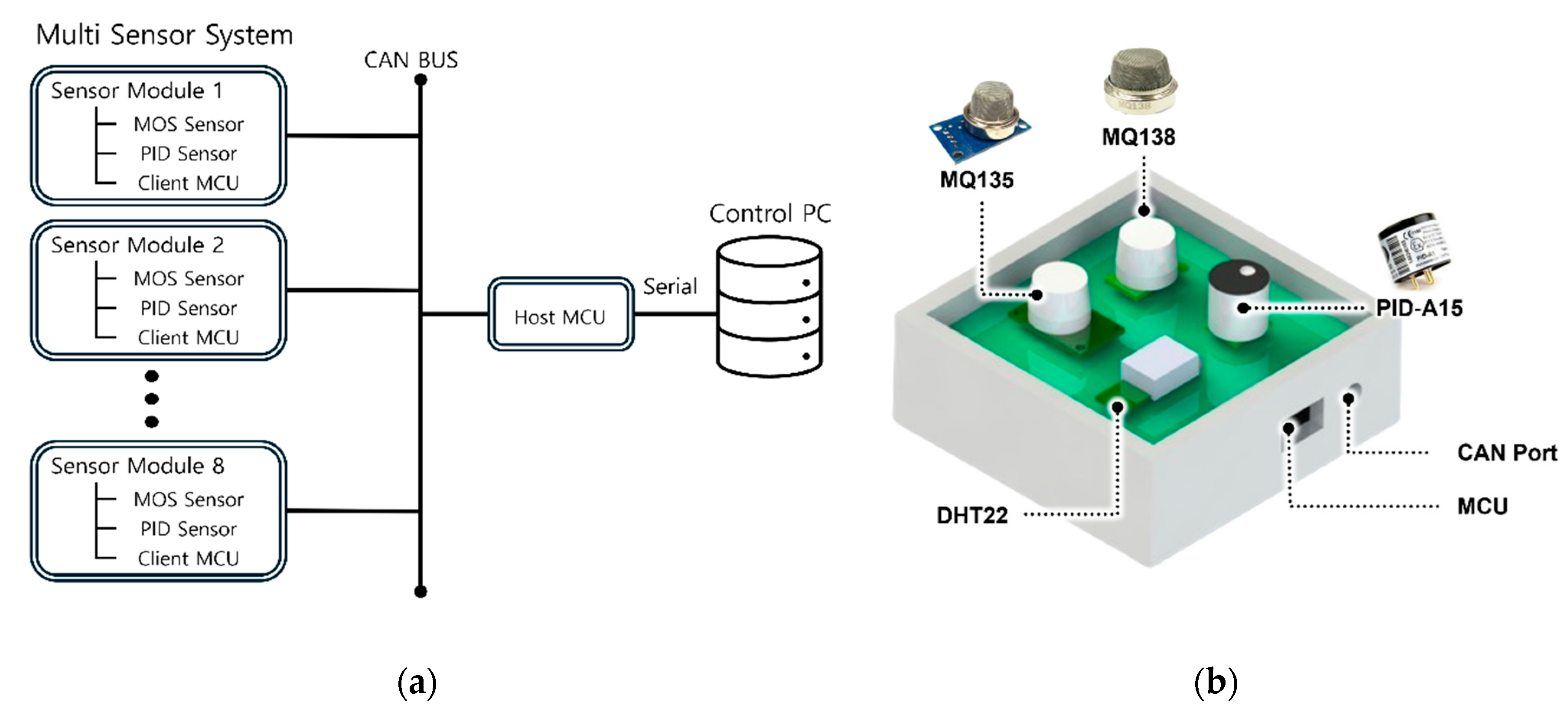
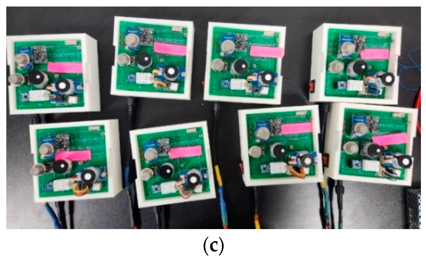
Figure 2.
Sensor module attachment position inside the chamber.
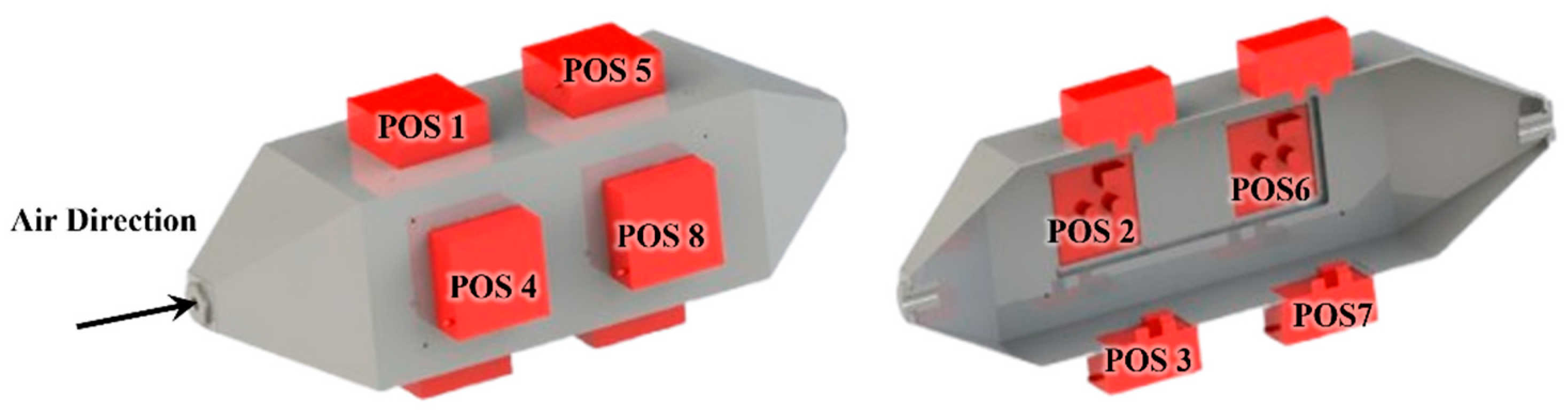
Figure 3.
(a) Schematic diagram of VOCs measurement sensor system experiments setting; (b) Setting of VOCs measurement sensor system.
Figure 3.
(a) Schematic diagram of VOCs measurement sensor system experiments setting; (b) Setting of VOCs measurement sensor system.
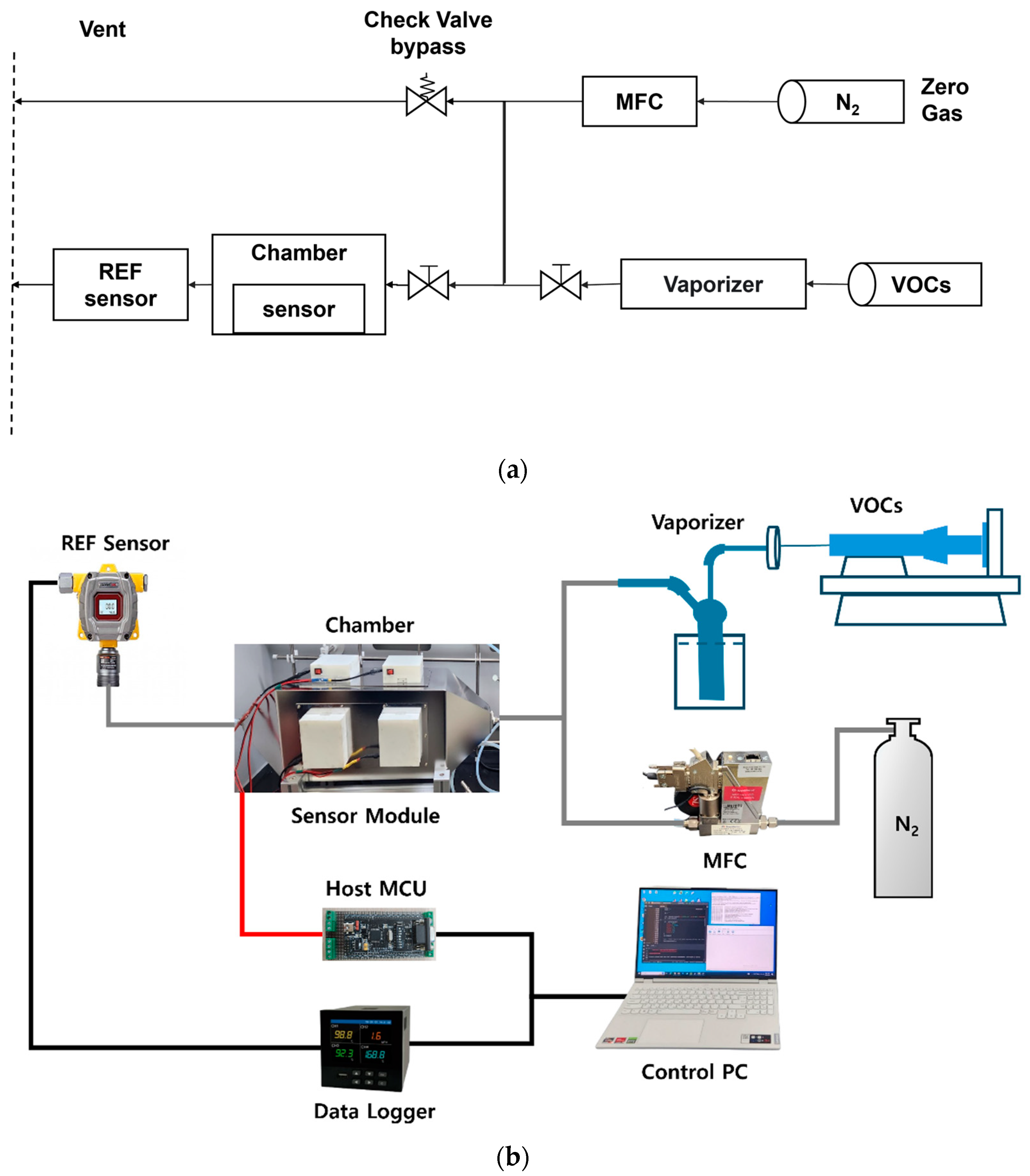
Figure 4.
Sensor 1 data after normalization of graph comparison (a) by up and down position and (b) by right and left position.
Figure 4.
Sensor 1 data after normalization of graph comparison (a) by up and down position and (b) by right and left position.
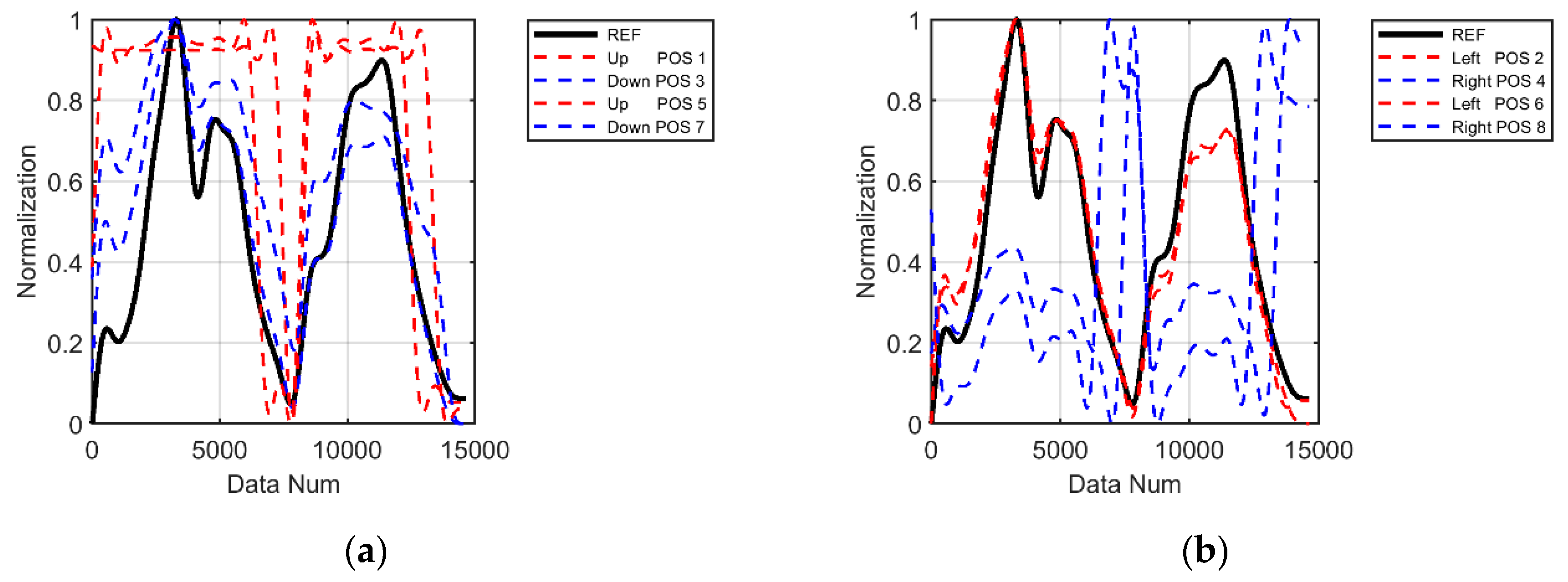
Figure 5.
Sensor 2 data after normalization of graph comparison (a) by up and down position and (b) by right and left position.
Figure 5.
Sensor 2 data after normalization of graph comparison (a) by up and down position and (b) by right and left position.
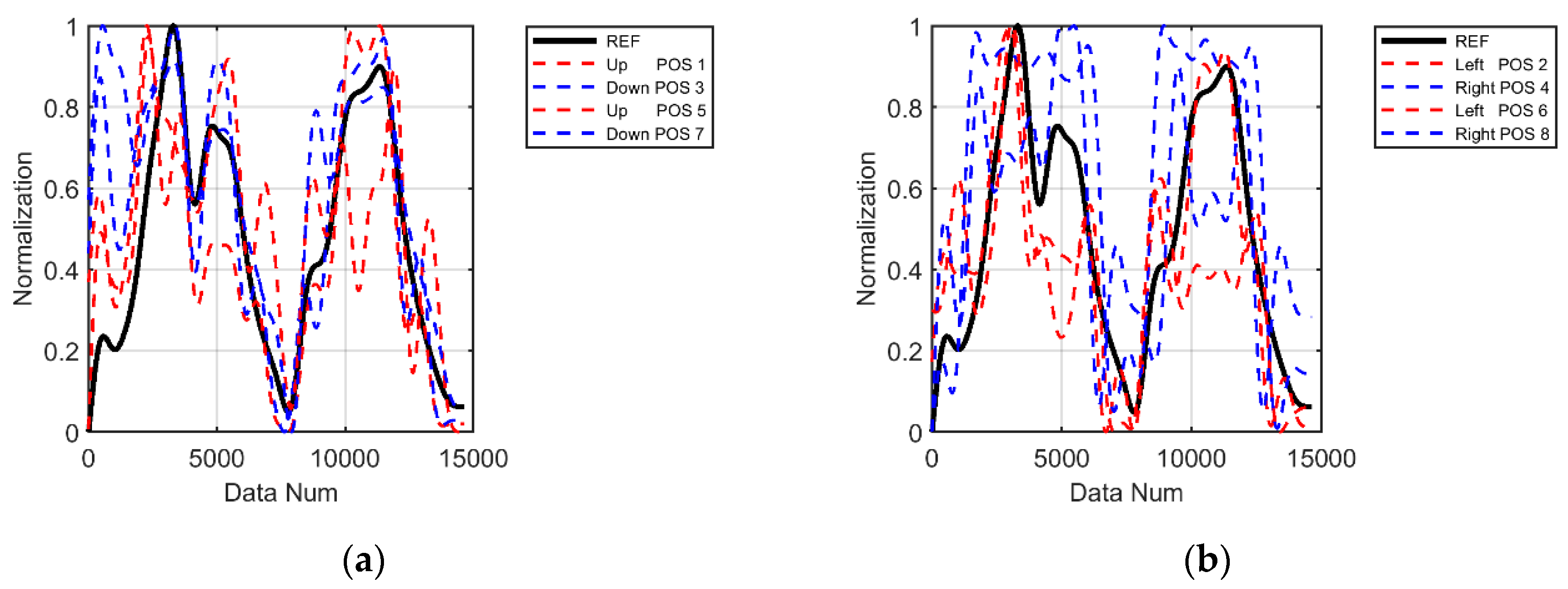
Figure 6.
Sensor 3 data after normalization of graph comparison (a) by up and down position and (b) by right and left position.
Figure 6.
Sensor 3 data after normalization of graph comparison (a) by up and down position and (b) by right and left position.
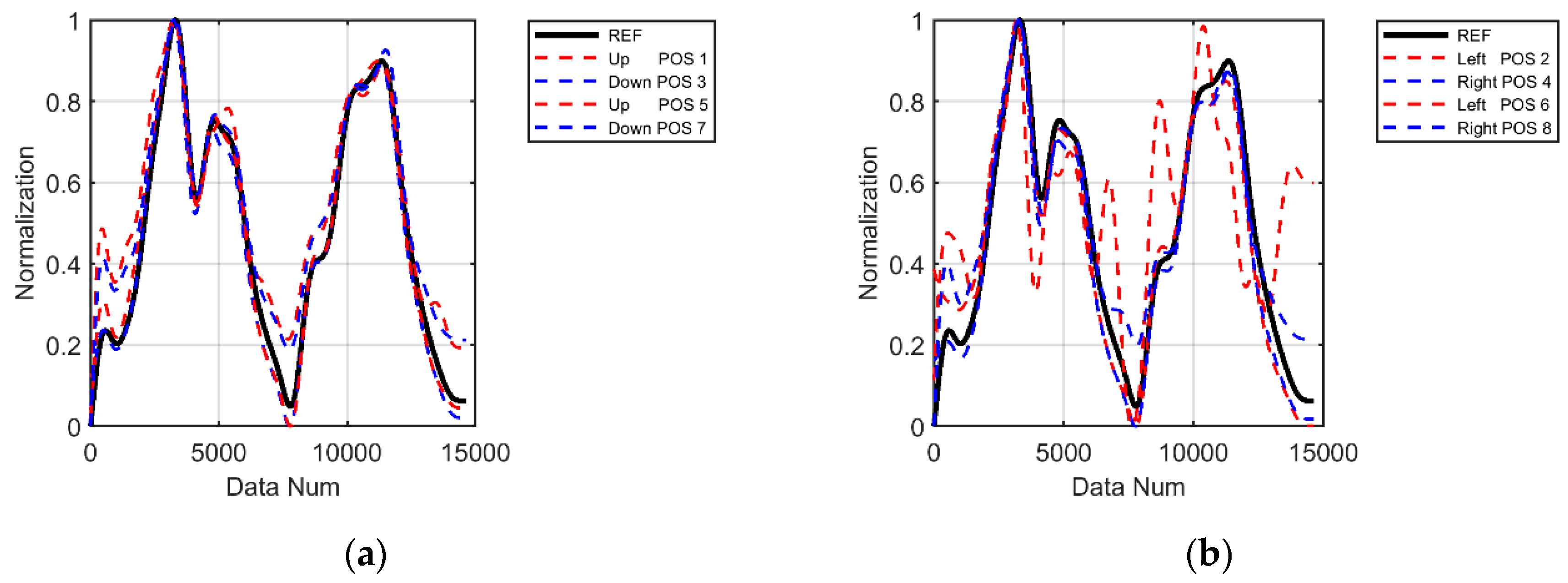
Figure 7.
Graph comparison by offset of (a) Sensor 1 (MQ135), (b) Sensor 2 (MQ138) and (c) Sensor 3 (PID-A15).
Figure 7.
Graph comparison by offset of (a) Sensor 1 (MQ135), (b) Sensor 2 (MQ138) and (c) Sensor 3 (PID-A15).
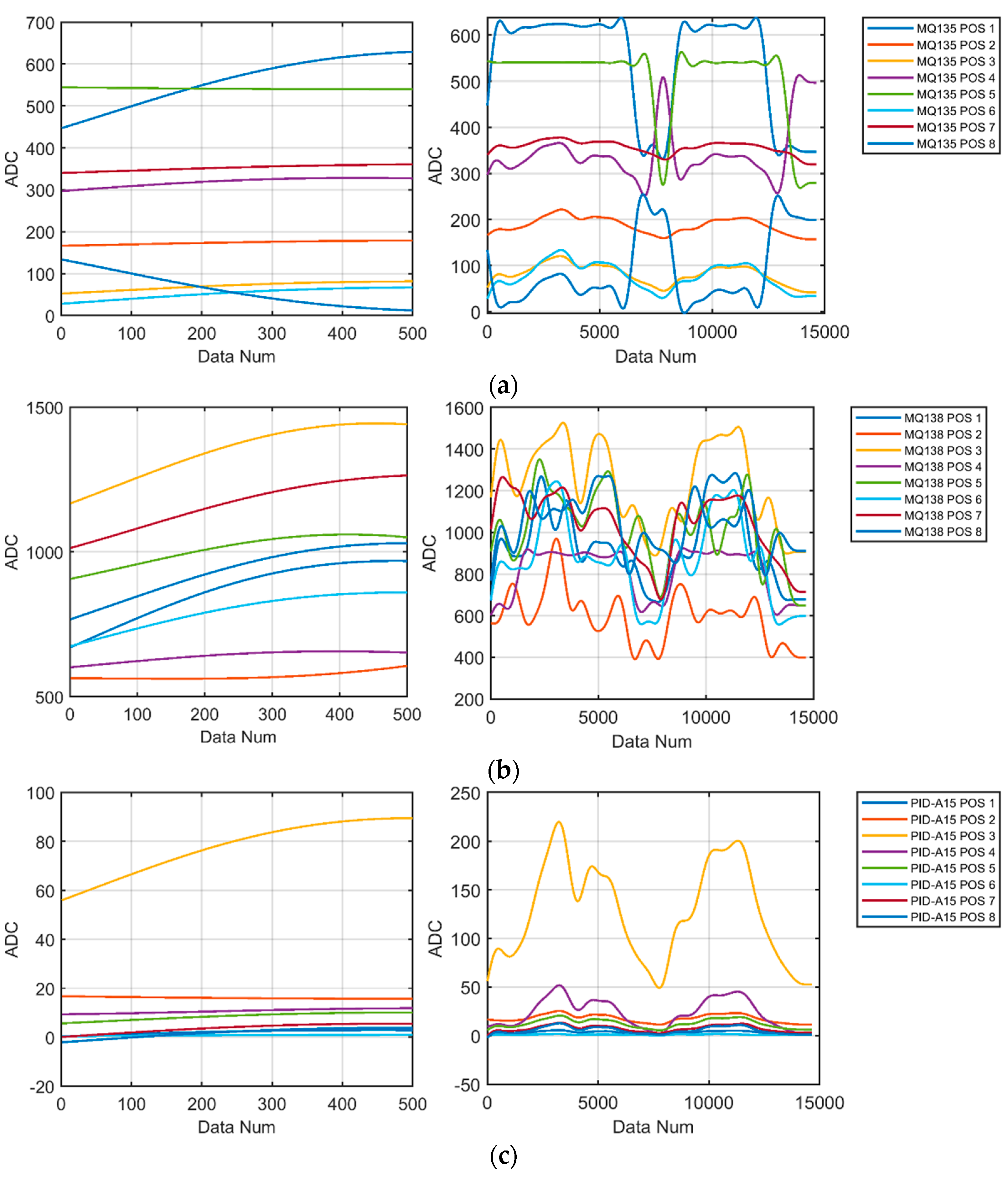
Figure 8.
ANFIS structure.
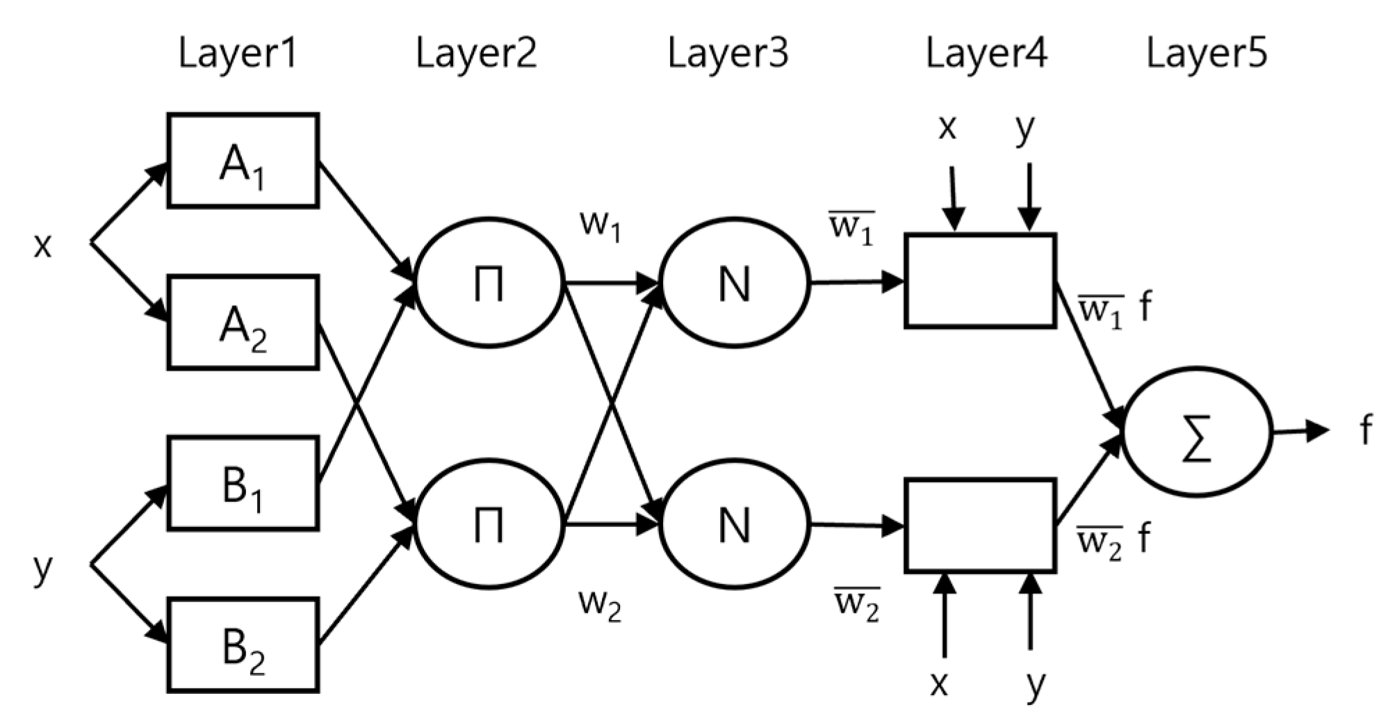
Figure 9.
Sensor 1 training error: (a) ANFIS training error for all positions, (b) ANFIS training error for sensors excluding the sensor with the lowest correlation and (c) ANFIS training error for sensors with adjusted outliers.
Figure 9.
Sensor 1 training error: (a) ANFIS training error for all positions, (b) ANFIS training error for sensors excluding the sensor with the lowest correlation and (c) ANFIS training error for sensors with adjusted outliers.
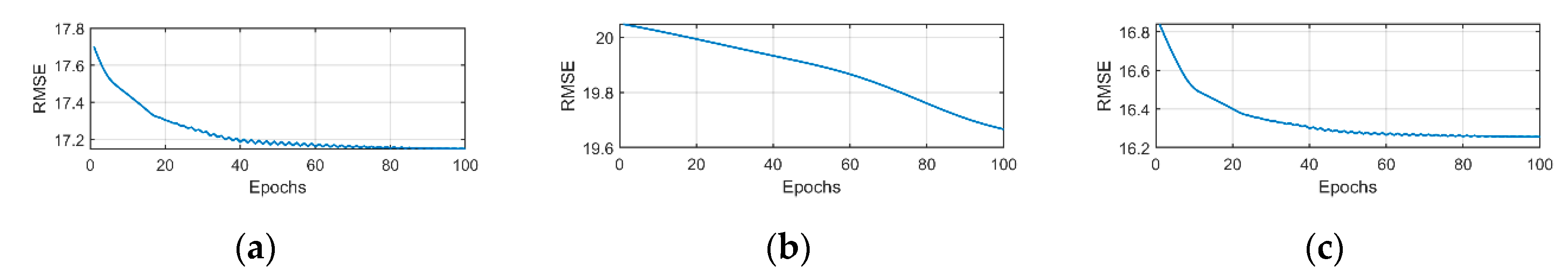
Figure 10.
ANFIS results for all sensors.
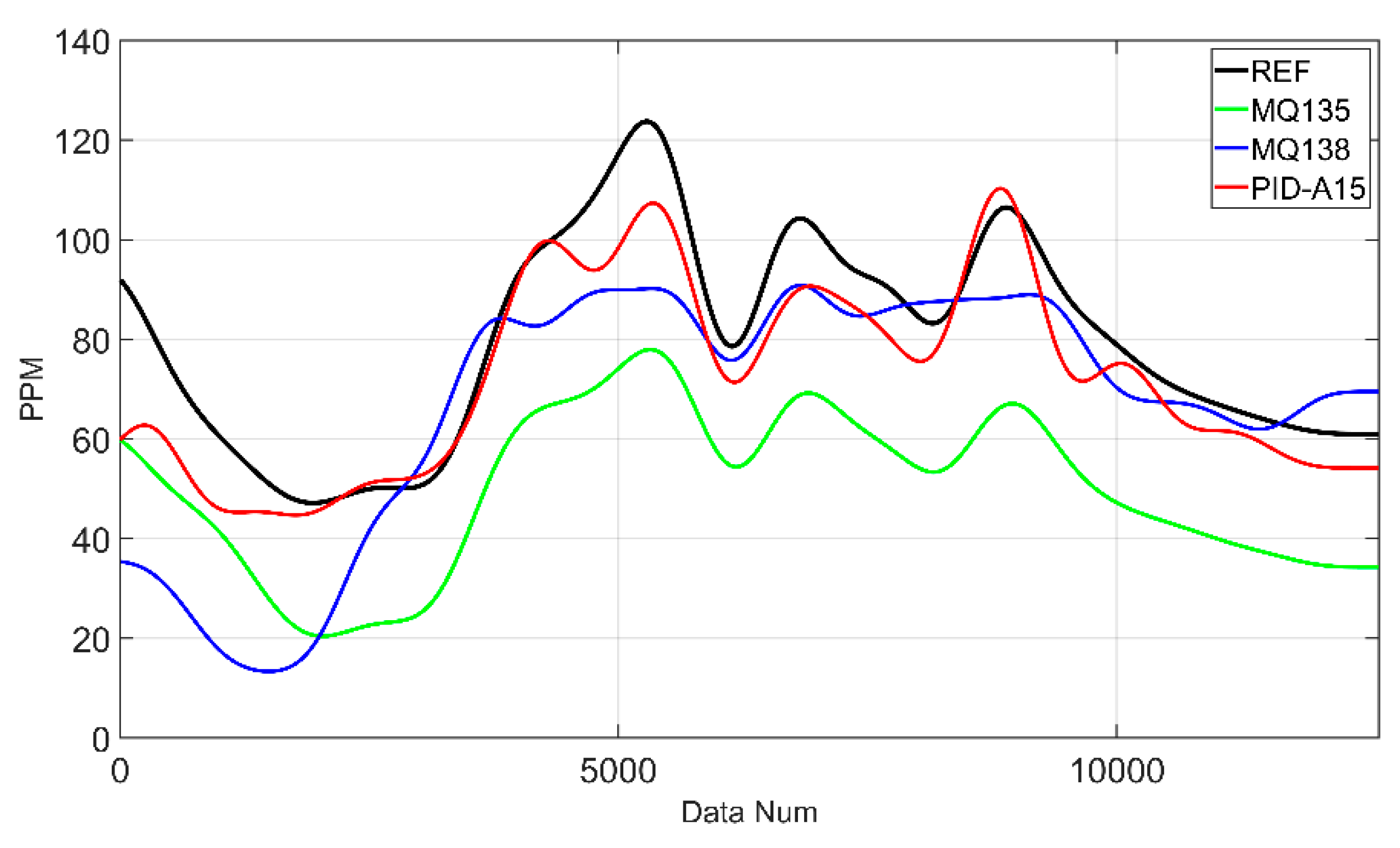
Figure 11.
ANFIS results for sensors excluding the sensor with the lowest correlation.
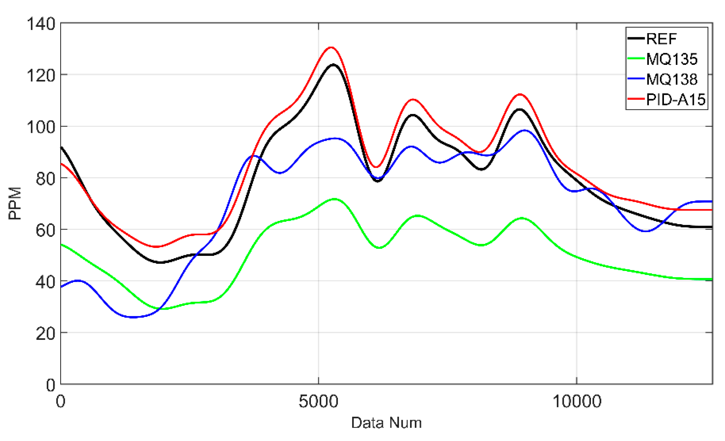
Figure 12.
Before and after outlier correction of (a) Sensor 1 data, (b) Sensor 2 data, (c) Sensor 3 data.
Figure 12.
Before and after outlier correction of (a) Sensor 1 data, (b) Sensor 2 data, (c) Sensor 3 data.
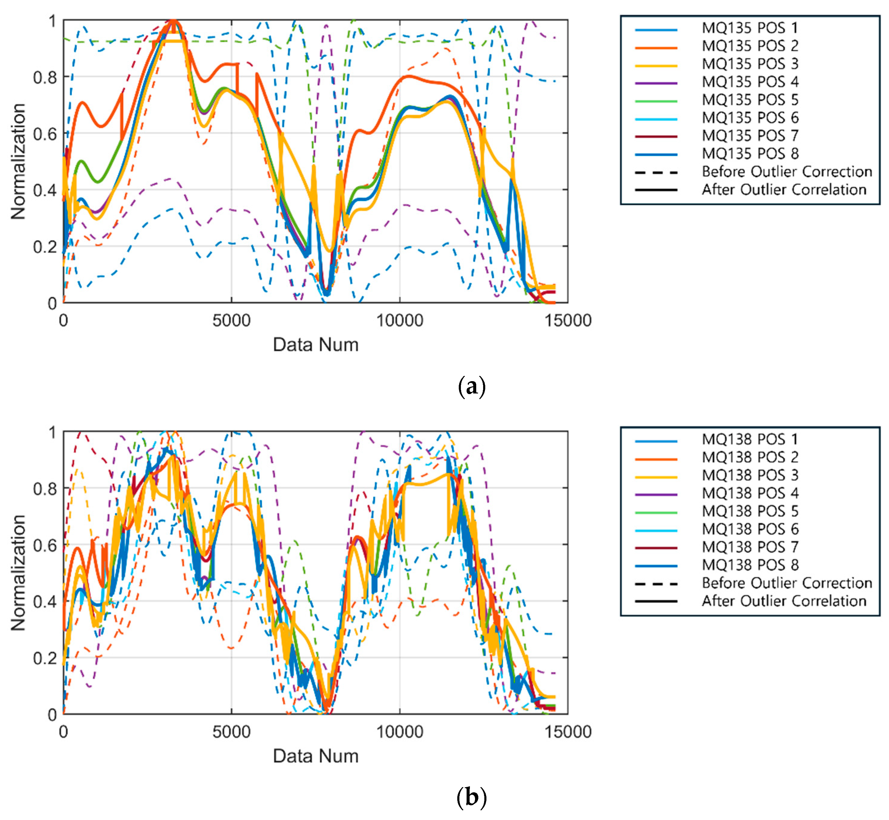
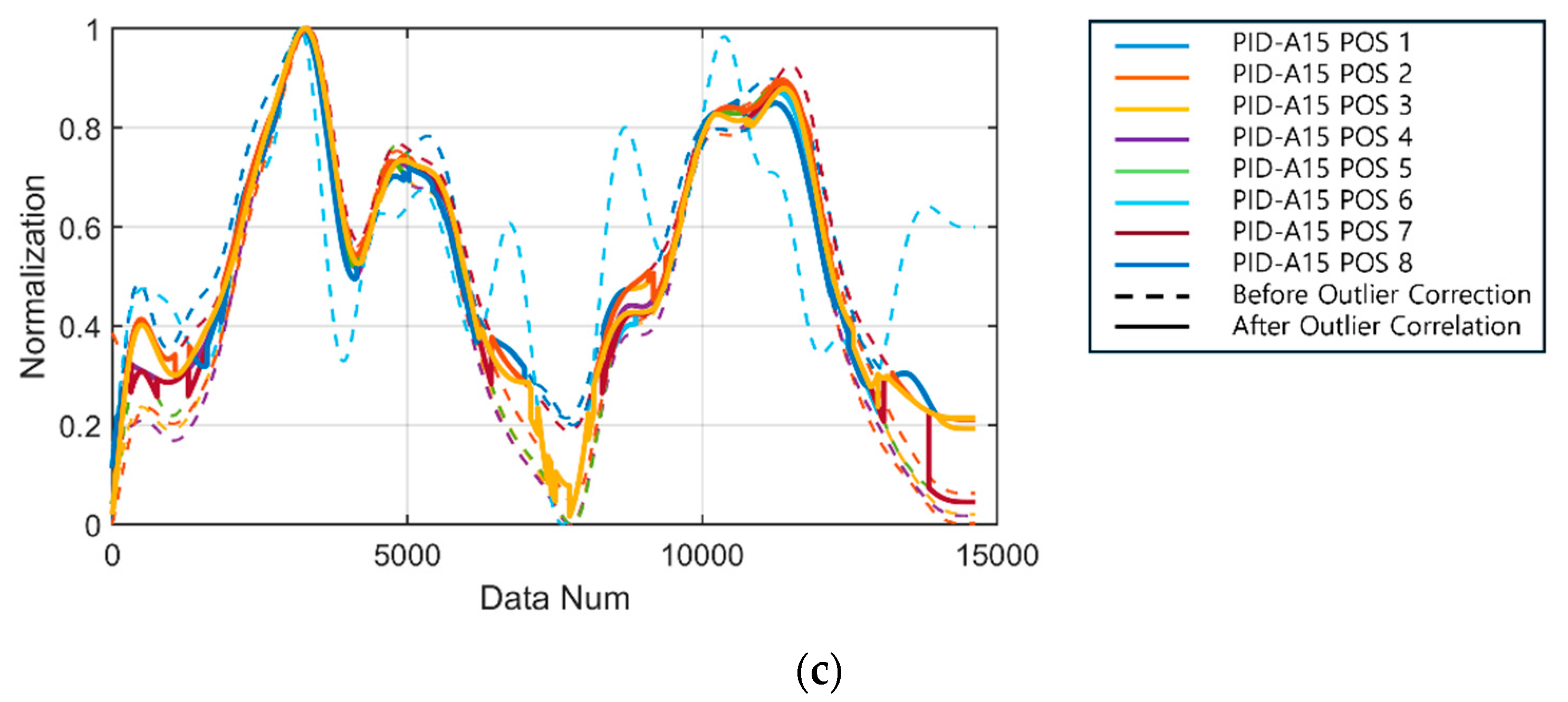
Figure 13.
ANFIS results for sensors with adjusted outliers.
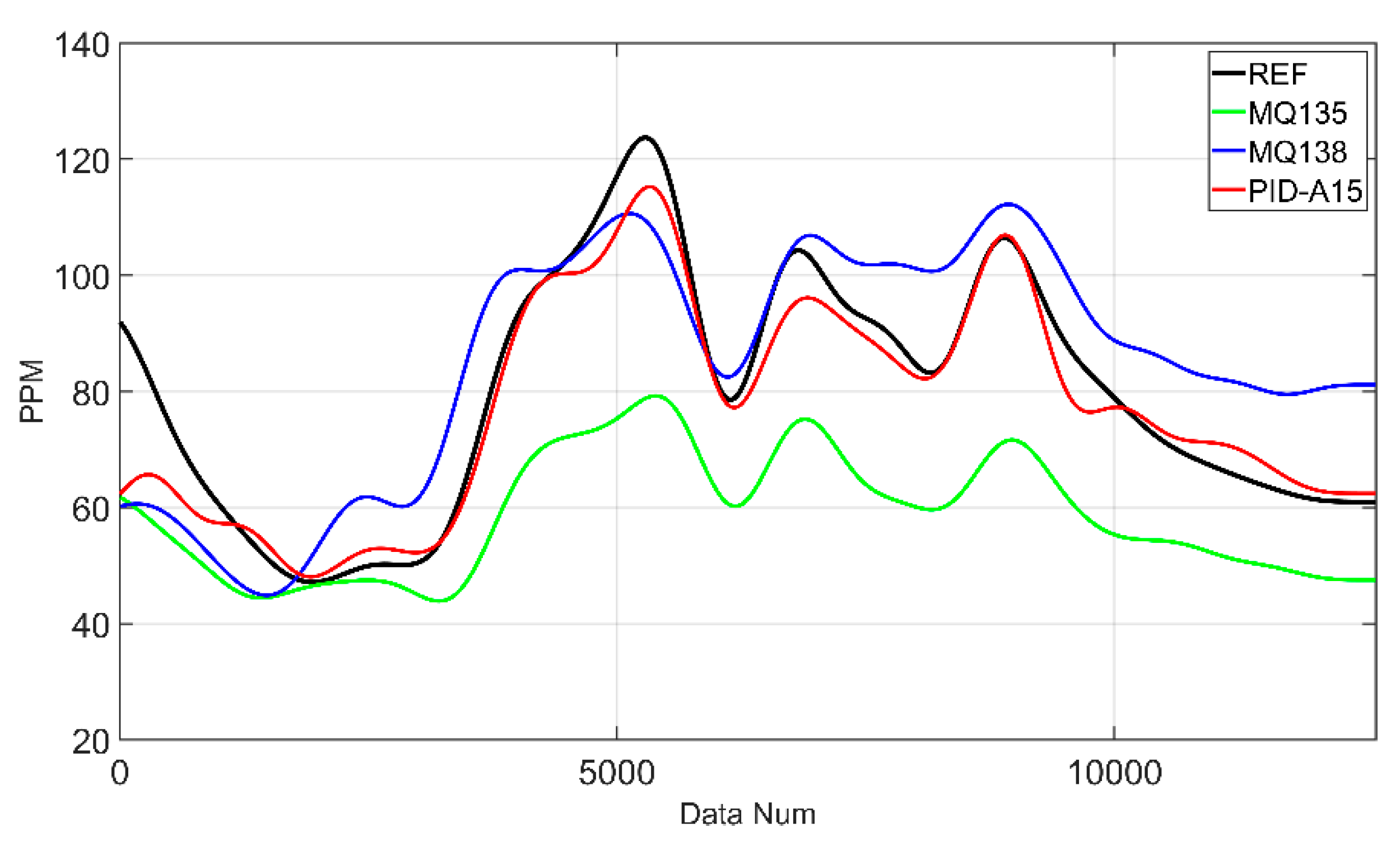
Figure 14.
RANFIS structure.
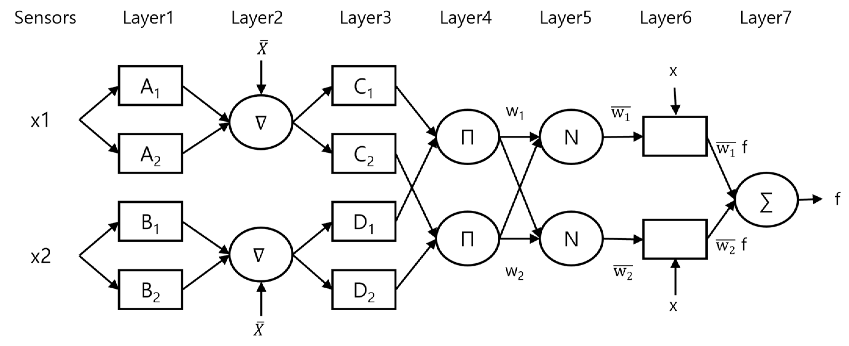
Figure 15.
Gradient compensation of (a) Sensor 1, (c) Sensor 2 and (e) Sensor 3 and reconstructed data of (b) Sensor 1, (d) Sensor 2 and (f) Sensor 3.
Figure 15.
Gradient compensation of (a) Sensor 1, (c) Sensor 2 and (e) Sensor 3 and reconstructed data of (b) Sensor 1, (d) Sensor 2 and (f) Sensor 3.
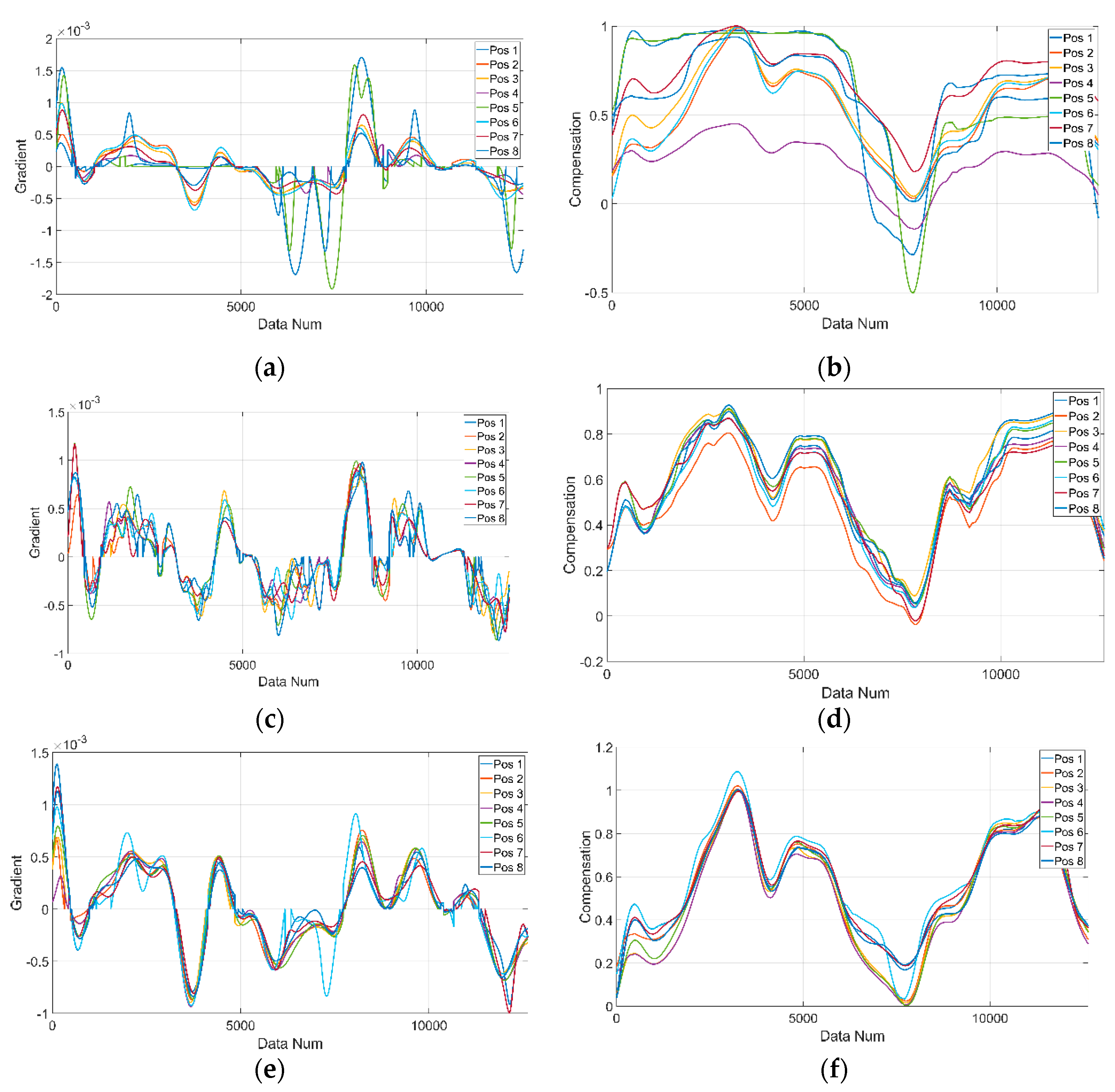
Figure 16.
REF sensor and ANFIS and RANFIS results for Sensor 1 data.
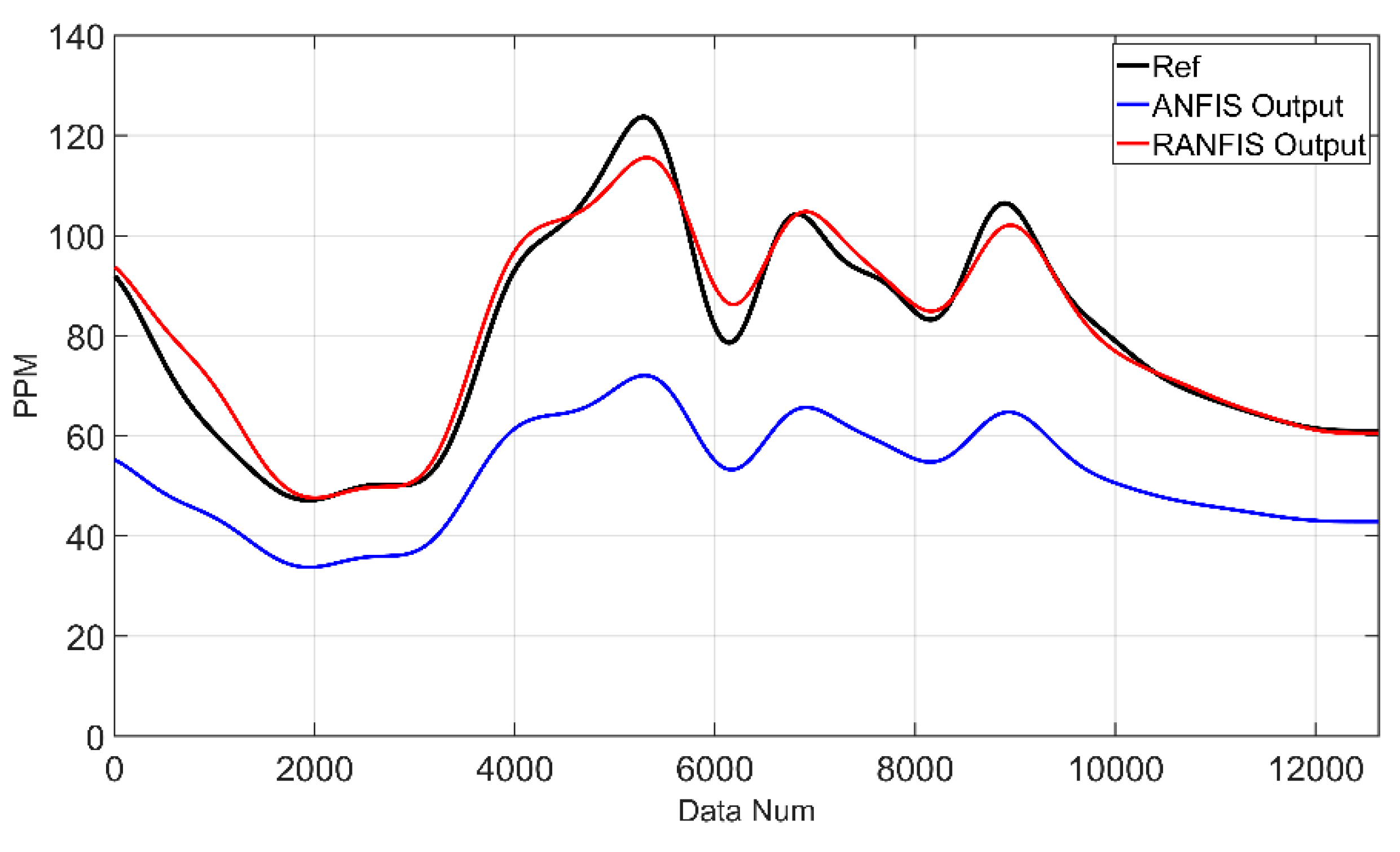
Figure 17.
REF sensor and ANFIS and RANFIS results for Sensor 2 data.
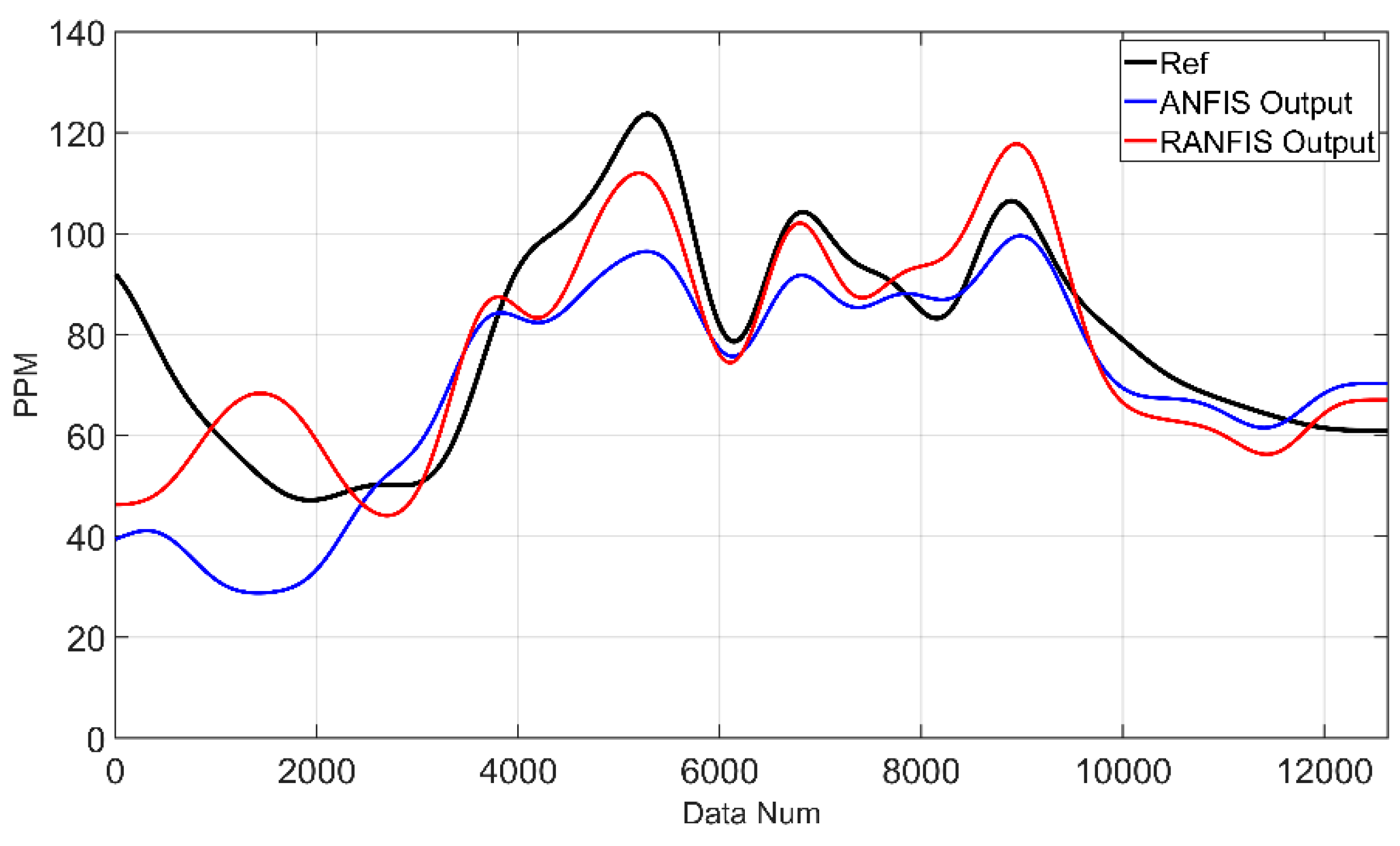
Figure 18.
REF sensor and ANFIS and RANFIS results for Sensor 3 data.
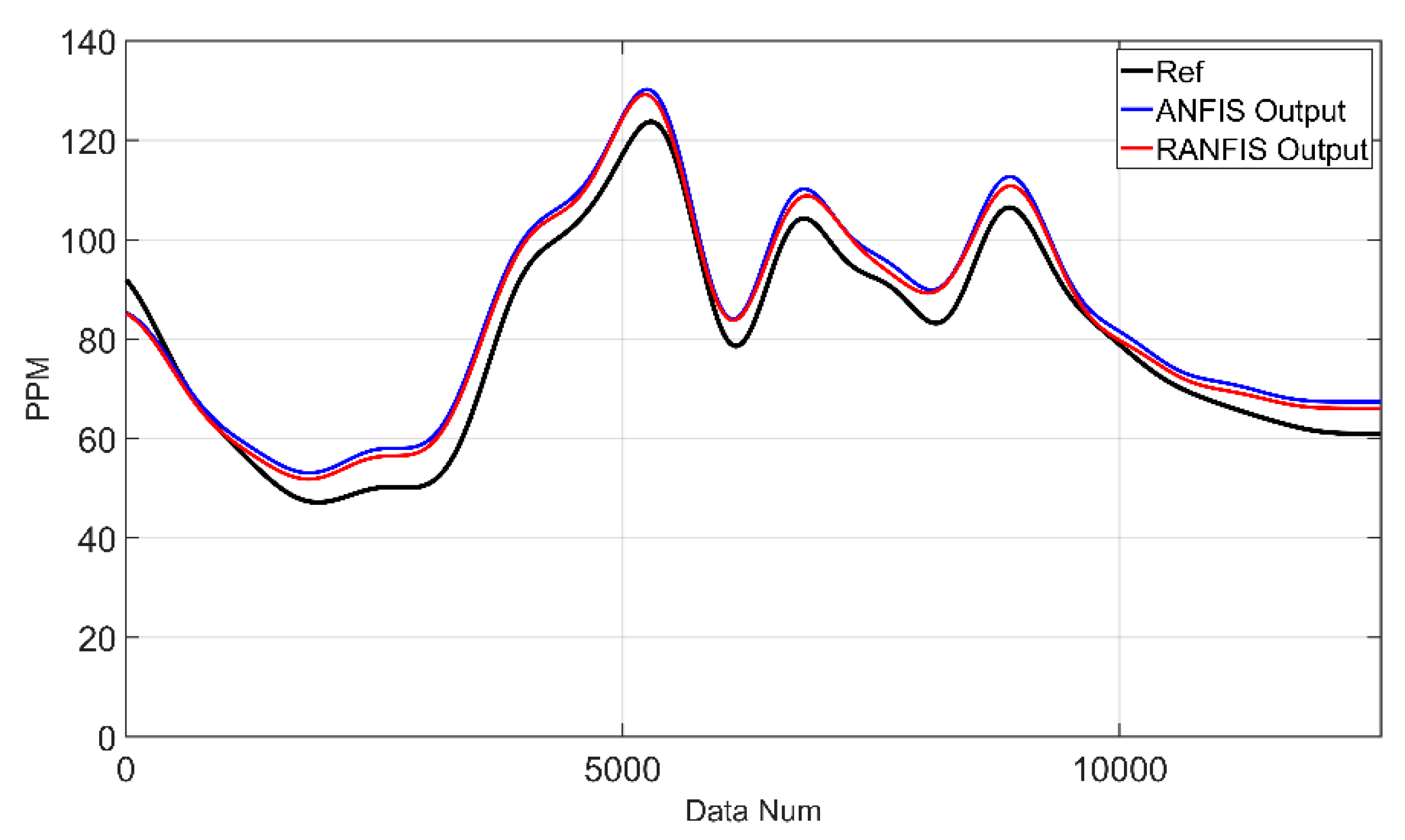

Table 1.
Low-Cost Sensors in Multi Sensor Module and Reference Sensors.
| Low-Cost Sensor | REF Sensor | ||||
|---|---|---|---|---|---|
| Sensor 1 | Sensor 2 | Sensor 3 | |||
| Model | MQ135 | MQ138 | PID-A15 | FIX800 | phx42 |
| Method | MOS | MOS | PID | PID | FID |
| Range[ppm] | 0 to 1000 | 0 to 500 | 0 to 4000 | 0 to 1000 | 0 to 100000 |
| Feature | Sensing Resistance 30K-200K |
Sensing Resistance 20K-200K |
Output variation with temperature ±5 |
Resolution 0.1 ppm Error ±3 |
Resolution 1 ppm |
Table 2.
Sensor 1 (MQ135) and REF sensor correlation coefficient and initial value by sensor position.
Table 2.
Sensor 1 (MQ135) and REF sensor correlation coefficient and initial value by sensor position.
| Sensor Position | Correlation Coefficient | Initial Value | |
|---|---|---|---|
| Up | Position 1 | 0.726554 | 447.4634 |
| Left | Position 2 | 0.950706 | 166.3442 |
| Down | Position 3 | 0.912168 | 52.2677 |
| Right | Position 4 | - 0.278603 | 297.1050 |
| Up | Position 5 | 0.570314 | 544.4116 |
| Left | Position 6 | 0.956624 | 28.1024 |
| Down | Position 7 | 0.846774 | 340.3473 |
| Right | Position 8 | - 0.562594 | 133.6359 |
Table 3.
Sensor 2 (MQ138) and REF sensor correlation coefficient and initial value by sensor position.
Table 3.
Sensor 2 (MQ138) and REF sensor correlation coefficient and initial value by sensor position.
| Sensor Position | Correlation Coefficient | Initial Value | |
|---|---|---|---|
| Up | Position 1 | 0.841348 | 670.6281 |
| Left | Position 2 | 0.603700 | 563.4451 |
| Down | Position 3 | 0.831878 | 1167.7626 |
| Right | Position 4 | 0.821266 | 601.3787 |
| Up | Position 5 | 0.682779 | 906.8697 |
| Left | Position 6 | 0.866885 | 674.7869 |
| Down | Position 7 | 0.681798 | 1013.5778 |
| Right | Position 8 | 0.639812 | 767.4062 |
Table 4.
Sensor 3 (PID-A15) and REF sensor correlation coefficient and initial value by sensor position.
Table 4.
Sensor 3 (PID-A15) and REF sensor correlation coefficient and initial value by sensor position.
| Sensor Position | Correlation Coefficient | Initial Value | |
|---|---|---|---|
| Up | Position 1 | 0.978340 | 0.3682 |
| Left | Position 2 | 0.968952 | 16.7813 |
| Down | Position 3 | 0.995301 | 56.0024 |
| Right | Position 4 | 0.993410 | 9.3810 |
| Up | Position 5 | 0.992887 | 5.6636 |
| Left | Position 6 | 0.631460 | 0.4201 |
| Down | Position 7 | 0.993589 | 0.1152 |
| Right | Position 8 | 0.987234 | 2.0791 |
Table 5.
ANFIS results.
| SENSOR | Sensor 1 (MQ135) | Sensor 2 (MQ138) | Sensor 3 (PID-A15) | |||
| RMSE | MAPE | RMSE | MAPE | RMSE | MAPE | |
| All | 30.406 | 38.826 | 20.319 | 20.247 | 9.635 | 9.466 |
| Remove LowestCorrelation | 30.351 | 36.049 | 16.394 | 16.245 | 5.871 | 7.491 |
| Adjusted Outlier | 23.491 | 24.451 | 12.595 | 15.359 | 5.703 | 4.793 |
Table 6.
Outlier proportion of the entire dataset.
| Pos 1 | Pos 2 | Pos 3 | Pos 4 | Pos 5 | Pos 6 | Pos 7 | Pos 8 | |
|---|---|---|---|---|---|---|---|---|
| Sensor 1 | 0.00 | 0.00 | 0.00 | 0.12 | 0.14 | 0.00 | 0.00 | 0.60 |
| Sensor 2 | 0.04 | 0.28 | 0.01 | 0.25 | 0.06 | 0.01 | 0.10 | 0.18 |
| Sensor 3 | 0.20 | 0.01 | 0.00 | 0.00 | 0.00 | 0.55 | 0.04 | 0.00 |
Table 7.
Quality score according to GAO proportion of the entire dataset.
| Pos 1 | Pos 2 | Pos 3 | Pos 4 | Pos 5 | Pos 6 | Pos 7 | Pos 8 | |
|---|---|---|---|---|---|---|---|---|
| Sensor 1 | 0.29 | 0.04 | 0.01 | 0.23 | 0.41 | 0.09 | 0.10 | 0.35 |
| Sensor 2 | 0.06 | 0.06 | 0.07 | 0.09 | 0.09 | 0.04 | 0.08 | 0.12 |
| Sensor 3 | 0.07 | 0.06 | 0.03 | 0.04 | 0.04 | 0.12 | 0.04 | 0.04 |
Table 8.
Comparison of RMSE, MAPE between ANFIS and RANFIS results.
| Sensors | Sensor 1 (MQ135) | Sensor 2 (MQ138) | Sensor 3 (PID-A15) | |||
|---|---|---|---|---|---|---|
| Model | ANFIS | RANFIS | ANFIS | RANFIS | ANFIS | RANFIS |
| RMSE | 29.215 | 3.758 | 15.654 | 11.594 | 5.854 | 4.837 |
| MAPE | 33.453 | 3.371 | 15.531 | 12.073 | 7.436 | 5.929 |
Disclaimer/Publisher’s Note: The statements, opinions and data contained in all publications are solely those of the individual author(s) and contributor(s) and not of MDPI and/or the editor(s). MDPI and/or the editor(s) disclaim responsibility for any injury to people or property resulting from any ideas, methods, instructions or products referred to in the content. |
© 2024 by the authors. Licensee MDPI, Basel, Switzerland. This article is an open access article distributed under the terms and conditions of the Creative Commons Attribution (CC BY) license (http://creativecommons.org/licenses/by/4.0/).
Copyright: This open access article is published under a Creative Commons CC BY 4.0 license, which permit the free download, distribution, and reuse, provided that the author and preprint are cited in any reuse.


