Submitted:
30 December 2024
Posted:
31 December 2024
You are already at the latest version
Abstract
In this review paper the equations of motion describing the fluid dynamics of the ionosphere are constructed step by step, so that any master or post-graduate student may get familiar with the general theory of the “traditional” approach to Ionospheric Physics, in which chemicals forming the Earth’s upper atmosphere are represented as fluids in mutual interaction. The hypotheses on which the smooth-field fluid representation is based are discussed in terms of microscopic dynamics of the gas particles: this discussion is oriented to prepare the reader for the post-fluid approaches to the physics of turbulence, to be treated in forthcoming manuscripts. The fluid dynamical picture of the ionosphere is the most classical and conceptually simple one, and this makes it extremely widespread in terms of theoretical models and applications.
Keywords:
Ioospheric physics
; Fluid dynamics
; Geophysical electromagnetics
; Classical physics
1. Introduction
The aim of this review is to present the general differential equations describing the Earth’s ionosphere system as composed by a certain number of classical fluids interacting one with the others in mechanical, thermodynamical and chamical way. Each of these fluids represents one of the various components of the ionosphere (ions, free electrons and neutrals). Mechanical interactions lead to energy and momentum exchanges. Thermodynamical interactions yield thermal exchanges of energy. Finally, the presence of chemical reactions allows for transformation of one fluid into another one via production and loss processes. Last but not least, elecromagnetic fields are generated by, and influence the dynamics of all those chemical species, many of which are electrically charged. The name we give to this system is generically ionospheric local medium (LIM), because its properties may depend on the position and on time t. Here the equations of evolution of the LIM are constructed step by step in great detail, taking into account for all the aforementioned aspects (mechanical, thermodynamical, electrodynamical and chemical) within a classical fluid approximation: through the concept of fluid parcel the dynamics is introduced keeping a macroscopic classical point of view, that does need suitable hypotheses of Statistical Mechanics, but does not stem from a particular microscopic dynamics and calculations on it. Great attention is payed to carefully expaining what all these approximations mean and what their implications are.
The review is organized as follows.
Section 2 is devoted to the rigorous definition of the system at hand and to the explanation of the approximations used.
In Section 3 the equations of motion are written down fully, including mass, momentum and internal energy balance for each constituent, plus Maxwell Equations for electromagnetic fields. Also, constitutive hypotheses are presented, to make the system closed mathematically. The dynamical system is formed by coupled partial derivative equations (PDE) plus constitutive hypotheses as contraints.
2. The System
The system of interest here is the Earth’s upper atmosphere, considered above the minimum quote at which the ionization due to Sun’s radiation or cosmic rays is so important to affect the propagation of electromagnetic waves [3]: this might appear a technology-centreed definition, but actually this “lower limit” coincides with the quote at which the atmospheric medium is active from an electromagnetic point of view, that is a rather intrinsic physical concept. All in all, our reasoning holds from approximately 60 km height up to the magnetopause of the Earth, in many different declinations. Actually, some authors refer to as “ionosphere” only to the electrically charged chamicals, i.e. ions and free electrons. Yet, as the equations of motion of these charged species do involve neutrals, and as the equations of neutrals can be expressed formally as those of the charged species, we are considering them as part of our system.
The reference frame used here is mainly the one co-rotating with the solid Earth, referred to as Solid Earth Reference Frame (SERF); sometimes it will be of use to introduce another auxiliary reference frame, namely the Neutral Wind Reference Frame (NeWReF), see below. Last but not least, the unit system used will always be the MKSA system.
The system of interest is neither a closed nor an isolated one [4]: it interacts mechanically and radiatively with what lies below it (lower atmosphere, lithosphere [5] and hydrosphere) and with the space environment surrounding the Earth (i.e., the solar wind, the Sun’s radiation and cosmic rays). The system does also exchange matter with what is below it and above it.
2.1. Smooth and Deterministic: The Continua
At a certain point of their history, physicists accepted that the world is made of very tiny systems, as molecules, atmos, electrons, and after all elementary particles, that render matter granular. However, since a couple of centuries at that moment, they had already developed a picture of macroscopic material systems as continua, i.e. extended distributions of matter occupying finite portions of the physical space and experiencing and applying forces all over their volume, and surface. From the invention of Calculus, physicists had given a precise mathematical meaning to the Latin proverb Natura non facit saltus, taken by Leibniz as a manifesto for modelling physical systems: any physical quantity should have a -dependence on the variables it is function of. This “phylosophy of non-roughness” applies to the description of continua stating that if a macroscopic continuum occupies a volume at a certain time t, any positional quantity describing its state (e.g., mass density, velocity, pressure...) must be a smooth field all over :
being the factor “” encoding the time dependence of and the mathematical set of values of (numbers, vectors, tensors...). In Figure 1 the assessment (1) is cartoonised: a greenish continuum evolves from an initial configuration to a later one through a supposed smooth evolution; this means that any local quantity describing it undergoes precisely the condition (1). Actually, considering the border of the sets the region where the local proxies of the continuum stop being defined, or may be understood to go from a finite value to zero “within no distance”, one should replace (1) with something more precise like (this does not, however, lighten the request (1)).
Despite its high requests on the mathematical description of matter reality, this picture has been able to give very satisfactory theories, as hydrodynamics, magneto-hydrodynamics, elasticity theory and many more [6]. Note that the picture satisfying (1) is also a deterministic picture, as the smooth time-behaviour of excludes noise from its time evolution, which is another very strong requirement.
Even if the continuous picture of macroscopic systems is very beautiful, yet at a certain point the granular nature of matter was experimentally proved, and in order to reconcile the latter with the smooth picture of macroscopic bodies some reasoning had to be introduced, namely the so called continuous limit of pointlike particle systems. The fluid dynamics (FD) of the ionosphere is one important product of this “ideology”, that has an elegant and effective resoning, but relies on precise and not-that-universal properties of the microscopic systems at hand.
The central concept of the continuous limit contruction is considering “small” portions of the continuum , referred to as parcels, and make the following reasoning (the term “small” has to be specified later). In such a there exist elementary components of the macroscopic matter system, each of which is moving with a certain velocity. In general, these components may or may not have all the same chemical nature, hence the same mass: the local representation of the neighbourhood within the continuum is obtained considering the centre-of-mass P of those components, to which the velocity of the centre-of-mass of the particles is attributed as . The local representation of the continuum at P is constructed starting by saying that the parcel of continuum moves with velocity . Figure 2 represents a cartoon of this idea. Recalling the definition of centre-of-mass, we may say that the point P is attributed the mass-average velocity of the particles within , i.e. the total linear momentum of the matter in .
The bridge between the micro-physics of particles and macro-physics of continua was traced by Statistical Mechanics, in which the macroscopic appearance of the world is conceived as the statistical sum of all the microscopic, fluctuating contributions of particles. Boltzmann’s Kinetic Theory paved the way for a quantitative study of those cumulative effects of what the micro-components are doing: this makes it possible to recover the local variables in (1) as suitable momenta of the statistical distributions of the particles in [7]: this is how mass density, bulk velocity, pressure, tension ... are defined in FD. This sounds quite intuitive, as we humans simply accept that our senses, and our classical instruments, simply sense the world of elementary particles “defocussing” their tiny details, and saving only a coarse-grained, average picture of it. In this reasoning, when one looks at the particles within the parcel of centre-of-mass P, the position mentioned in the FD fields is the position vector of P: in what follows, and P are used with the same meaning.
All in all, the macroscopic picture would be obtained via a “statistical” way:
being some physical quantity depending on the single particle variables, and a sign of suitable statistical averaging(whatever this may mean at this early point) performed within at time t. In order to rely on a statistical procedure as (2), one needs a first important ingredient to the very existence of the s: the number has to be so huge to point towards the Thermodynamic limit
This is the first tough requirement to go from particle physics to FD, that had become a necessity once molecules, atoms and all their tinier fellows were discovered. In any statistical theory, due to results as the Central Limit Theorem [8], there is the need of having enough samples to be able to neglect stochastic fluctuations, that is precisely what one needs to do in order for to be a deterministic (hence, time-smooth) process. Note: the condition (3), that may sound definitely sensible considering a small glass of water to contain s of molecules, is not at all obvious when one would like to represent the physics of galaxies (made of “few” solar systems) or even a finite portion of very dilute space plasmas (made of “few” p and ) with FD, in which the constituents are all but s of bodies. In those cases, the theory of small thermodynamic systems, large fluctuations and extreme events have to be invoked [9].
Once we have defined the continuum quantities as non-fluctuating fields on , one has to have them smooth, as prescribed by (1). This means that, if one has two “nearby” points P and within separated by some “small” displacement , as in Figure 3, one has to be able to calculate the non-fluctuating value as , the non-fluctuating value , and then find the incremental limit between them with respect to the distance to exist:
Equally, there must exist also the limit
defining the instantaneous rate of change with time of . Actually, the two requirements (4) and (5) demand for differentiability of in space and time, while the requirement (1) is extremely stronger because it means to have infinite space and time derivatives: clearly (1) imply both (4) and (5). More cleanly, one could replace the two requirements (4) and (5) getting the whole (1) by assessing
the differences between at two (macroscopically) nearby points or at two nearby times must scale to zero as positive integer powers of the distance or of the time lapse considered. Clearly, this (6) rules out any turbulent regime of classical fluids [10]. In (4), (5) and (6) the symbol refers to a length in the set of the valus of , for instance the absolute value for real numbers, or Pitagora Theorem norm for three-dimensional vectors.
The construction of the continuum representation of a macroscopic system of matter is all pivoted on the definitions (2) satisfying the conditions (6), starting with the definition of a velocity field as described before and sketched in Figure 2, and a mass density field , defined for the matter in as the ratio , being the total mass of particles forming , and the parcel volume. Defining these and helps us explaining how “small” the “parcel” must be taken around P: reference is made to the idea of macroscopic infinitesimal portion [11], for which one starts to ideally shrink the volume in around P and applies the definitions to smaller and smaller volumes ; at a certain size of one stops seeing and fluctuating, while go on with shrinking too much, fluctuations re-appear. At the beginnig of this “plateau” of the values with decreasing one stops including in the parcel regions of the continuum in different local conditions; when fluctuations re-appear at too small values of , the number is not satisfying the condition (3) any more, and the granularity of matter is unwantedly appreciated in terms of fluctuations.
Concluding this rapid introduction to continua, that is the necessary foreword to FD, we refer again to Figure 2: the set of particles in have their degrees of freedom, three of which have been taken into account considering the position of P and the velocity : these are the centre-of-mass variables [12]. What about the other degrees of freedom, namely the variables relative-to-P, e.g. the difference between the position of each of the particles of and that of P, and their canonically conjugated momenta?
Treating also this huge number of relative variables is necessary to completely describe che phase space of the particles in the parcel, but despite it is sensible to use the per se deterministic variables for the centre-of-mass P of the parcel, being the total momentum of , the relative variables of the parcel will be treated in a statistical way. That is: while is already a field as those involved in equations (1) and (2), the positions of the particles in the parcel relative to P and their conjugate momenta become the subject of the -local statistical mechanics. As the dynamics in this relative phase space
is treated statistically, becasue , the statistical distributions on become the completion of the description of the exactly particles in .
On a theoretical ground, describing statistically the relative variables within the parcel vmay consist of the dynamics of the Gibbs distribution in [7,13]; in practice, one always assumes the particles in to be represented by some kinetic theory that will cut the BBGKY hierarchy in to 1-particle distributions. Moreover, as the only well established statistical mechanics is equilibrium thermodynamics, the -local kinetic theory will converge to the definition of local thermodynamic variables attributed to the point of position vector , as new smooth fields . All in all, the microscopic degrees of freedom of the particles in the parcel will turn into the 3 ones of the centre-of-mass plus an equilibrium thermodynamics for the relative coordinates, representing the inner structure of , converging however to some other local smooth continuum system variables (e.g., the pressure, or density, and temperature, see SubSection 3.4 and Section 3.5).
With this, the FD philosophy of the LIM is established; before moving on focussing on the system composition, let us resume it in items:
- the system is formed by parcels with thermodynamic numbers of particles (3);
- the statistical mechanics of these particles converges to space- and time-differentiable emerging variables (6);
- the system is locally in thermal equilibrium, hence described via a kinetic theory converging to a local equilibrium thermodynamics.
The requirement 1 makes it possible to have well defined non-fluctuating statistics tout court; the requirement 2 leads to the feasibility of deterministic smooth FD at all. Last but not least, the requirement 3 is the path leading to FD as we know it today. The thorny debate about physical regimes when those requirements do not appear to be met deserves future manuscripts.
2.2. The System: Matter and Interactions
Let us now introduce how all this theoretical background is applied to the Earth’s ionosphere.
The system is considered to be formed by S chemical species, indicated as , with . For example, molecular species as O2, N2, CO2, NH4, but also atomic species as O and N, are in this list. If the neutral species considered are
and the ion species are
then the example composition reads:
In the ionosphere, these S chemicals are in the state of gases. Each of the different gases is an extended system of matter represented as a continuum in the way discussed before, i.e. with parcel dynamics: at each point P of the space a parcel is considered for the I-th chemical, with a centre-of-mass velocity and the I-th relative phase space described via statistical mechanics, in general, more practically via P-local equilibrium thermodynamics.
This is only the matter part; there is a field part too, made of those fundamental force fields acting on the atmospheric gases: gravity and electromagnetic fields. Due to the average speeds of the subsystems in the SERF, and to the energy of the processes treated, here we represent everything in terms of classical physics, involving only small sips of Special Relativity, here and there, when the electromagnetic fields are to be transformed from a first observer to another one. Gravity will not be a dynamical variable of the system!
Every component experiences the action of the gravitational field defined around the Earth, which includes the field of properly massive origin, the inertial positional forces and the time varying field due to the tidal action of other celestial bodies. From a General relativistic point of view one should include Coriolis force too in the gravitational field, while here the Coriolis force will be kept as separated from the whole “effective” gravity. In general one can write:
Coriolis forces are thus due to Coriolis acceleration field
being the rotation vector of the Earth as seen in a frame in which this Coriolis force is not experienced, and the fluid velocity of the I-th species, constructed as explained before.
Electromagnetic fields are experienced only by charged continua (in the example (7) the ions and and the electrons ), and for these particles their strength is much more important than that of gravity. In general there is the geomagnetic field , that is considered as a rigid external field, and some non geomagnetic, perturbing magnetic field , due to temporary phenomena (e.g., the geomagnetic storms), so that one has
Many electric fields of different origin are also present, and this will be clarified later.
Quite the opposite to what happens to gravity, the electromagnetic fields acting on the s undergo important back reactions due to charge displacements, net currents and dynamoes produced by the motion of these fluids. The “complete” dynamical system we will deal with will then include all these fluids plus the fields and influenced by the atmospheric motions (it should be stated that the mechanics of the s are only a part of the source of the atmospheric and , since is generated, in its component in equation (9), by some conducting lavic movement inside the solid Earth [14]).
2.3. Fluid Matter Variables
Every single chemical component is described as made of particles of mass and electrical charge , we will use to indicate mass density, for numerical density and for charge density. These quantities are related as:
Of course, , and are proper fluid fields as the discussed in SubSection 2.1.
The components involved can be neutral species
or charged ones
In ionospheric studies the use of is often preferred instead of , because the numerical densities of particles enter the typical expressions of cross sections, determining the production and loss rates of the s in chemical processes, and also because the expressions of many measurable quantities are entered by the numerical density of free electrons. For what concerns one must say that the functional relationship (10) renders it practically equivalent to or for the charged species, while when it simply vanishes.
About these s, in general a constraint of neutrality of the LIM
may exist, besides the global one:
The constraint (13) is a standard in many applications of ionospheric physics, even if particular regions, as the dawn and dusk terminator, may violate it.
Local thermal equilibrium is assumed for each : then, temperature fields will come into the play; it is useful to remember that the different chemicals have different temperatures, they are not in thermal equilibrium with the others; for example, electron temperature has been measured as about , while positive ions were found around in the polar E layer at about 150 km height, when intense electric field are present, as reported in [15]. This should not be surprising, despite the different s are in thermal contact with each other: as they are moving, floating and interacting, these gases are in a well different condition from that of fluids in a calorimeter. This also keeps the system far from a global thermodynamic equilibrium.
The continuous approach, which is largely valid for studying plasma and neutrals of the “standard” ionosphere, can not be used to describe the rain of high energy particles entering the Earth’s atmosphere from the space, because of the hypothesis of local thermal equilibrium which is lacking for them.
2.4. Dynamical Variables for Matter
A fluid occupying a certain volume in the space is fully described when point by point and time by time its velocity field, mass density and tensions are given [16]; this means that for each constituent one should use the -vector
(bulk velocity given by the centre-of-mass velocity of the parcel with the centre-of-mass in ), the -scalar
(bulk mass density) and the distinct elements of the stress tensor
with , a two rank -tensor. Usual fluids as those at hand have symmetric stress tensor, so that one has 6 independent components . This , plus , plus give all the fields to describe each continuum composing the atmosphere in the Eulerian picture. However, tensions are not further variables to be added to and : the s are in general functionally dependent on the velocity field , and “fluids” are classified into different species according to the mathematical form of the dependence
The tension dependence on velocities is restricted in general to a particular subdivision of , that can be written as the sum of a pure positional addendum and on another term depending on the s too:
The continuum is defined as fluid if
holds. In the very particular case in which
one speaks about ideal fluids. The definition (20) means that the system is not able to exert any off diagonal stress when it is at rest. The statement (21) indicates as ideal fluids those fluids unable to exert off diagonal stresses also when they are moving.
The -scalar in (19) is the hydrostatic pressure. The case of perfect fluids well represents the s in very dilute regions [17]. Note that since is a scalar under the rotation group it must be related to the trace of , so that is traceless.
In order to describe energy exchanges the thermodynamical nature of the system must be taken into account; then another quantity is introduced, the local temperature , which is also an -scalar. The full set of dynamical variables we have introduced to describe each is then given by the density , the velocity , the pressure , the tensor and the temperature , giving a set of 12 unknowns in the equations of motion. In SubSection 3.4 the roles of and will be clarified from a fully mechanical point of view, as coarse grained proxies of the microscopic degrees of freedom of the matter of the fluid at hand, contained in the volume , in terms of variables relative-to-the-centre-of-mass of the “parcel”.
The various fluids are generally classified and studied as follows [18]:
-
Neutral particles. Various molecules or atoms (e.g. O, N, O2, N2, CO2, NH4 and so on) with zero electric charge: these ones are the major part, both numerically as well as massively, of all the high atmosphere, up to the level of about 1000 km height, starting point of a region where practically all the matter is ionized. From that point on, one speaks about plasmasphere.If each neutral species is indicated with the index , the speed of their centre of mass is point by point some field , defined as follows in terms of partial matter densities and velocities :This velocity undergoes a proper dynamics that may be attributed to the neutral matter as a unique fuid .
- Negative ions. These are the species which have captured one or more electrons. These particles are very rare and their presence is practically negligible in general. Nevertheless, one should consider them when dealing with the lower part of the ionosphere, as the region D and the lower E [19]. Negative ion abundance is reasonably non negligible only under 95 km, even if in particular conditions this can be false. Sometimes a coefficient is defined for each negative ion asgiving the measure of the contribution of the species to the ionospheric negative charge, relative to the electron one.
- Positive ions. These are the neutrals that have lost one or more electrons: actually, the 2- or 3-valent positive ions are very rare, so we can restrict to the study of 1-valent positive ions. When the constraint (13) holds and no negative ions exist, positive ions have a numerical density equal to that of free electrons.
- Electrons. Electrons are the most important element for ionospheric phenomenology as far as electromagnetic disturbances are concerned, because of their very small mass that gives them a great mobility [3], making them very effective in producing local and travelling electromagnetic fields.
In general one could represent in a Lagrangian way the fluid motion as the evolution of a manifold, a domain continuously filled in with matter, and describe its motion as the transformations undergone by this manifold. The manifold can stretch, roll, it can be deformed by tensions, its centre-of-mass moves under the action of external forces. Basically one physical portion of it can be identified as the evolution of a fixed portion of the initial continuum [16]. This way of representing the evolution of a continuous system has led to a Hamiltonian description of fluids alternative to the local approach (for reference see [20,21,22] and [23]).
In the absence of chemical reactions the mass of the parcel remains constant:
being the operator making the time derivative along the motion [24] . What happens if chemical reactions take place? When chemical reactions enter the fluid dynamics, it is convenient to treat the systems as non constant mass systems, writing:
This is the variation rate of the mass of the parcel as following the parcel motion, and it can be either positive or negative, according to production or loss processes.
The description of the fluid is referred to as Lagrangian or substantial, because the quantities used refer to the degrees of freedom of a material portion of the system ; on the contrary, fluids are often described in the Eulerian or local way, in which one describes the situation via quantities thought of as properties of the spatial point at hand [16]. When some quantity is attributed to a fluid, the relationship between the Lagrangian version and the Eulerian version of it is given in terms of time derivatives, and reads
being the local speed of the fluid to which is attributed (for ionospheric continua, the s and in (26) have a chemical species index I)
It has already been stated that the extended system has centre-of-mass (CoM) variables and relative-to-CoM (R2CoM) variables as explained in [12] and references therein. The evolution of the CoM variables will be governed by Newton’s principle as explained in SubSection 3.3 below. For what concerns the R2CoM variables,a statistical approach is used for them in ordinary fluid dynamics, see better SubSection 3.4.
2.5. Electromagnetic Dynamical Variables
The mathematical tools describing the system are completed when the variables used for the electromagnetic fields are given. At each point in the space around the Earth an electric vector and a magnetic vector can be given, both time as well as position dependent:
These electric and magnetic fields are obviously governed by Maxwell equations. While there exists a Lagrangian description of fluids with a straightforward interpretation, electromagnetic fields do have only an immediate Eulerian dynamics: this is why all the -dynamics is reformulated in local terms, through the translation (26).
In general, the electromagnetic field in a point of interest will be the superposition of many fields of different origin.
The magnetic field is given by the superposition of a “permanent” geomagnetic component , that is generated by sources in the interior of the solid Earth, and other “temporary” terms, indicated collectively as in (9). is not constant on the long term, because it has been proved to vary: roughly speaking, it is some dipole magnetic field that slowly rotates and changes its shape. At Italian latitudes and longitudes, for instance, it is representable as a rigid dipole migrating of about one prime per year. Actually, this dipole is not rigid, and its motion should be studied in a complex theoretical way (see [14] and references therein). However, the variability of this takes place on times which are too long compared to the processes usually discussed in LIM modelling.
The inclusion of a field in the system at hand as a dynamical variable depends, by the way, on the inclusion of its sources: since we decided not to include the currents inside the solid Earth in our system, we will regard the geomagnetic field generated by them as an external constant field . On the contrary, the part can be affected by ionospheric or magnetospheric sources.
The electric field is generally produced by charge separations related to the motions of the ionospheric plasma. In many cases this can be considered as slowly varyingwith time, and treated as electrostatic, and so a potential giving is introduced.
3. Equations of Motion
The equations ruling the motion of the atmospheric system are essentially those of classical Newtonian physics, plus thermodynamics, plus classical electrodynamics.
For the electromagnetic fields the four Maxwell equations will be used directly, while for what concerns the matter part, conservation principles applied to the parcel dynamics will drive the reasoning.
3.1. Mass Balance
The mass balance is written for the I-th species by considering that each of the many species present in the atmosphere undergoes creation and destruction due to chemical and photochemical processes. Neutrals are “destroyed” in ionization and “reconstructed” due to recombination of electrons and positive ions, or detachment of electrons away from the negative ions. In the same way free electrons are created in ionization together with positive ions, in the detachment processes of negative ions, and destroyed in general in attachments and recombinations. Finally, positive ions are created together with electrons in ionization processes, and destroyed in recombinations.
In general the mass balance can be obtained by elaborating equation (25): if the parcel of the I-th element is some which occupies a volume , and the mass density is , one can write:
The total derivative is applied as
and all we have to do is to write as a function of the matter degrees of freedom presented in SubSection 2.4: the physical quantities we will involve in our discussion are the density and the velocity of the parcel.
The density is already involved explicitly in (28); one has to evaluate in terms of the parcel velocity. The variation of the measure can be calculated considering that the measure of changes due to the motion of the points on its surface , so that this time derivative is the outgoing flux of this speed:
When Stokes theorem is applied to this integral one has
Considering the smallness of , it is possible to write:
Placing (30) into equation (28), we can write:
The mass source term can be imagined as proportional to the total mass of the parcel as , because each particle in the parcel may undergo the same chemical reactions with the same probability distributions, so that may be written as:
being the mass of the single particle of the I-th species and the source field suitably defined in (32). This expresses equation (31) involving the Lagrangian derivative of
and going from the Lagrangian to the local expression of , one has:
The total space derivative
is recognized, then equation (33) turns out to read:
It is useful to write the source term as the difference
between the local rate of production of the I-th species, and the corresponding rate of loss . Equation (34) is then re-written as:
Each species has its own loss and production term in (36), but these are not all independent; their forms encode the chemical processes taking place in the ionosphere, that have the elementary constituents of the continua as reagents or products. These reactions undergo some conservation relations, and the source terms in (36) must satisfy those conservation laws. The matter of the total system
must have constant mass (under the hypothesis that no nuclear reaction takes place, and considering not to discuss the loss or gain of chemicals due to some matter exchange with the near-Earth space). This means that there must exist a total mass balance equation with zero source,
where is the total mass density of the multi-fluid system and is “the right vector” to take part to equation (38) (being the “right vector” to be defined few lines below). The way of deducing the total equation (38) from all the particular equations (36) is straightforward, it suffices to sum them all and define accordingly, that will turn out to be rather intuitive. Summing all the equations (36) over the chemical species, one gets
Total quantities are recognized straigthforwardly: firs of all, the total density
while transport terms give the right addendum in (38) when is defined so to satisfy:
This is a well known quantity in mass kinematics: is as the “speed of the centre of mass” for all the fluids. Due to these definitions, we have
If equation (41) has to coincide with equation (38), enforcing the mass conservation, we must have
that is the mass conservation condition on the production and loss terms and The equation (42) is a basic condition for aeronomical chemistry, claiming that chemicals are not created or destroyed “out of the blue” or “into nothing”, but simply turned the ones into the others. The only external contribution to this apparently closed system balance is the supply of energy from solar photons, that are destroyed when photochemical processes take place. Yet, these photons will not be recognised as a futher species of chemicals, essentially as long as chemical, and not nuclear reactions take place, so the energy of these massless photons will not be translated into mass.
The constraint (42) is not the only condition one has to fulfill when writing the production and loss terms. Conservation of the electrical charge must be taken into account, as well. In order to get the charge conservation condition, let us go back to (36) and divide it by , that is clearly a constant parameter. What one gets is
Conventions (10) give
that is the balance equation for number densities. This equation (43) is the key continuity equation for any additive quantity held by the single fluid species: an example of such quantities is indeed the electric charge. Equation (43) is multiplied by the I-th electric charge
and definitions (10) are turned to again, so that:
If is the total electric charge density of the whole system of fluids, then one would like to get
and this is obtained by summing all the equations (44) as and recognizing
This gives
so that if equation (47) has to be equivalent to electric charge conservation, the following condition on the s and s
must be realized.
In general, if an extensive quantity H exists and has density for the I-th continuous species, and total density
one can define its total current as
The single species balance equation for H reads
being the amount of H carried by the single particle of the I-th species. This yields
giving finally
as a “total H conservation condition”.
3.2. Chemical Space Formalism
A particularly suitable symbolism for fluid with dynamics, loss and production processes, is referred to as vector chemical space formalism.
There is one equation (36) for each chemical species, let S be the total number of chemical species. Let us rearrange the mass conservation to involve the numerical concentration instead
then let us think that these S equations are the components of the following system:
(where , , and are S-component real vector in the “space of chemicals”: in equations (54) and (55) the summation over is intended in the terms and . Summations take place over repeated indices in contravariant positions). The local conservation constraint (53) for any conserved quantity H is read as an orthogonality relationship in between the collection of the values and the collection of the source terms:
The equation (55) is referred to as species-vector continuity, and its components are coupled via the source term that satisfies (56). In fact, this source term depends on the densities
and maybe on the time and position explicitly, so that equation (55) all in all reads:
In order to understand equations (57) in a general way, we must classify explicitly the properties of the function , its possible symmetries and the simplifications. Turning back to the components , we can appreciate the various levels of coupling between different species by expanding in the densities, via a simple Taylor series approach, e.g. up to the third order:
(the following reasoning makes an exact sense as long as has a convergent Taylor series, otherwise it is just an approximation). When such expressions are put into (54)
one discovers that the various terms involve zero, one, two, three, ... species of particles, and thus correspond to chemical processes with zero, one, two, three, ... chemical involved. It is not said that in the n-th order term n different species are involved: in fact, there are terms in in which a given can appear with a degree higher than one. These different momenta of in the space of species must form a function which satisfies the constraint (56): putting (58) into it, one has
The various terms must be zero each, because we are setting to zero a polynomial in the components of . For the zeroth order one has
which essentially means the impossibility of creating charge in the empty space, with . One can see in Chapman ionization theory in [3,17] an explicit application of this. For example, if our model atmosphere is represented by the three species X, and , equation (61) reads
that is
3.3. Momentum Balance (Newton’s )
The fluids composing the system described at the beginning of this Section are made out of point particles that essentially obey to Newton’s principles. In the approximation described in SubSection 2.3 the initial condition Cauchy problem
for a particle of mass m can be transported to the continuous system of the I-th constituent as the Navier-Stokes equation [7], that is exactly Newton’s Second Principle, or equally the linear momentum balance, written for the parcel.
The linear momentum of the parcel is some , so we have
If its mass is referred to as and we use the symbol to indicate the force experienced by this , we can write:
stressing again that is the velocity of the centre of mass of the parcel at hand. From equation (25), this can be written as:
The mass of the parcel reads
and considering also the definition (32), equation (65) can be written as:
The volume element can be factorized on both sides of (67) by defining
so that all in all one has
This (69) will be written in local terms by applying (26) to the fluid velocity itself, so to obtain
In order to enumerate the forces composing we have to list those systems acting on the portion of fluid. The parcel interacts with the following systems:
- the electromagnetic fields and defined at its position;
- the gravitational field defined at its position;
- the inertial forces measured in the reference frame co-rotating with the Earth (the SERF);
- the remaining part of the system which interacts with at the border through the nearby parcels;
- the other systems with ;
- the mechanical waves passing by the position of .
Let us come to the complete expression of the force : as announced before, let’s assume that is a generic charged fluid and let’s attribute to a total electric charge
This charge makes experience a force due to the presence of the electromagnetic field, that is written in Newtonian terms as
being the fields those defined in SubSection 2.5.
The second force acting on is the gravitational force, represented as
the field is obtained in the SERF. It is basically composed by the Kepler-like gravitational potential given by the rest mass of the Earth, plus the positional part of the inertial forces due to the Earth’s motion. If the angular velocity of the Earth is supposed to be constant within the time scales treated here, we can say that includes and the centrifugal force:
The Coriolis force is calculated for the parcel of mass and velocity as:
The force applied by the rest of on the under exam through the border of the small volume can be expressed as an integral over the surface of the outward flux of an -tensor of rank 2, referred to as the tension tensor; this has been indicated in SubSection 2.4 as , and one can write:
being the infinitesimal element of the area of and the outward pointing versor locally perpendicular to . From Stokes theorem one can write
that can be approximated as
as tends to zero. When the symbol is used for the tensor variable whose components are the , the force may be written as
In general equation (19) holds, and divides into a pressure part and a viscous part. When this is put into equation (76), one has
The forces due to the other systems are viscosity forces that can be seen as the friction due to the motion of the parcel through the viscous medium . Let the velocity of be at the position of the parcel : if the time frequency of collision between an I and a J particle at per unit mass is some , the friction force is
then the total friction force due to the systems reads
The last system interacting with can be anymechanical wave field travelling through the atmosphere. When such a wave goes across the space it carries momentum and energy, and can exchange these quantities with whatever it meets. In particular, this may be conveniently as the divergence of a tensor , so the volume force applied by a mechanical wave reads:
We are finally in the position of writing the force completely, getting rid of the infinitemal volume , as:
Equation (81) is the Navier-Stokes equation for theI-th fluid involved in the system, and it is clearly coupled with all the other fluids , and with the electromagnetic fields. One may work with the number densities of the chemical species, putting (10) into (81):
Wherever the I-th element is present and this can be furtherly written as
The sum of the two tensor terms is often referred as a unique term , so that
As is mainly a friction term, the in (84) is generally referred to as general viscosity tensor.
3.4. Internal Energy Balance
The quantities as , or refer to the “inner structure” of , that is composed by particles. As the parcel does contain order of Avogadro number of particles of the I-th chemical, it is considered a thermodynamical system, its physical variables undergo thermodynamical relations: then , and will be involved in an internal energy balance
where U is the internal energy, is a portion of energy thermically exchanged and is a portion of work. The signs in (85) are chosen so that is the heat acquired by the system, and is the quantity of mechanical work exerted on the parcel [25]. It is very important to underline that the energy balance we are speaking about is a thermal balance: we are not discussing about the energy that releases or incorporates due to its centre-of-mass motion throughout the space; here we deal with energy exchanges that concern the internal degrees of freedom of the mechanical system treated in terms of equilibrium thermodynamics of the particles of the parcel (this is why equation (85) does not contain any potential energy term due to mechanical work made by external conservative forces on the centre-of-mass degrees of freedom, i.e. no gravitational or electrostatic energy term). The inner structure of is mimicked again in Figure 4
Let us consider the three elements , and and write them in terms of the degrees of freedom of . These quantities , and are variations/increments happening while the parcel CoM moves along the trajectory during some time of a displacement . This means that is for example the Lagrangian variation of the internal energy of the parcel , so that:
In order to write correctly we must first of all think that it is a function of volume and temperature of the gas to which it refers:
One can write its value working on the volume-temperature plane starting at some point with the same volume of the parcel, and integrate along an iso-volumic trajectory
being the energy at the point , and its temperature. Due to this expression, the variation on the left hand side of (86) must be carefully calculated as
It is possible to make this derivative when all the time dependences are carefully considered: this is done in Appendix A. All in all, the result turns out to read:
A little argument requires a comparison between this (89) and the expression (86): in equation (86), is not a scalar field in the physical space, but a function of the parcel degrees of freedom relative to its centre-of-mass. When the expression (87) is introduced one just put in evidence this thing, making depend on and t through the temperature , so that the mathematical framework to arrive to the local representation is gained. What one must keep in mind is that the thermodynamics of just depends on the local position through belonging to the parcel of CoM equal to at time t.
Let us turn to the term of thermal exchange of energy between the parcel and the environment. Three mechanisms of heat exchange must be considered: thermal conduction , due to temperature differences between the and the nearby parcels; mechanical dissipation due to interaction with the environmental part of (and related to the tensor ); heat internal production and dispersion due to other processes, more explicitly discussed below:
Let us examine these addenda one by one.
The quantity of heat exchanged by the parcel due to thermal gradients can be expressed as the integral of the heat current all around the surface : considering that the heat spontaneously flows from warmer to cooler regions one can write
being the thermal current, and the I-th thermal conductivity. The integral in (91) is positive when points from inside to outside the surface , so that the environment being hotter than the parcel will give a positive to . Mathematical symbols in (91) are the same as in (76). Transforming the surface integral in (91) via Stokes theorem
and considering the smallness of the material parcel, one has:
The quantity is indicated in general as
In a similar manner we introduce a quantity so that
The total heat contribution is included in the equation (85) of internal energy as:
Let us now examine the work term: consider that this infinitesimal work is the portion of work made by the environment onto the thermodynamical degrees of freedom of the parcel in the time . In particular, is the expansion work made by varying the value of :
(this expansion-compression work is different from the acceleration of the centre-of-mass of : the latter would be calculated through the power of the external forces applied to the in the momentum balance). Equation (30) leads to:
and the internal energy equation is finally added to (81) as a proper equation of motion
The whole set of “fundamental” equations involving the matter degrees of freedom can be displayed as
which give us PDEs. The unknowns involved in them are more than five, anyway, let us remind that they are
for each fluid, giving quantities for each . Some more relationships must be added, in order to have a well posed problem.
3.5. Some More Relationships
The next relationship useful to get as many equations as the dynamical variables is the angular momentum balance for the parcel , that actually gives some useful aid. Indeed, the fact that there must be angular momentum conservation in fluid dynamics leads instead to some constraints on the stress tensors, that should be symmetric for the matter systems [16]: actually, this reduces the components of from 6 to 3. We are then left with being 9 unknowns, while the system (98) contains just equations.
The fundamental equations for fluids are all in (98): writing them we are finished with exploiting the general laws concerning every kind of fluid. This means that in order to obtain a number of equations equal to the number of matter unknowns, one has to start with particular hypotheses defining the special kind of fluid one is dealing with.
First of all, since we are treating the parcel of the fluid just like a thermodynamical system, we can turn to thermodynamics to find other useful equations. When the hypotheses described in SubSection 2.3 for the classical continuous description hold, we can say that the system is locally near its thermodynamical equilibrium, it has a well defined state (represented by and ), and evolves by undergoing quasi-static transformations. As long as local thermodynamical equilibrium is supposed, some equation of state will hold and the tension , the density and the temperature will be constrained to fulfill some relationship of the form:
(as discussed in [1], this may not be always the case; in general the local equilibrium hypothesis is consistent with smooth dynamics). In general the ionospheric fluids and the thermosphere are assumed to be ideal gases [17]. For a volume V of moles of ideal gas one has
when the system is the parcel one has and is the ratio between the mass of and the molar mass of the I-th gas :
When the Avogadro number is involved the equation of state turns into the following form
being the Boltzmann factor. Then (99) reads
Equation (99) adds one relationship to the five equations in (98): then we have 6 conditions, 5 PDEs and 1 constraint, one the 9 variables , 3 more equations are still needed.
Other important relationships rising the number of useful equations up to 9, and thus eliminating the underdetermination question of the boundary problem given by (98) plus (99), are provided by the dependence (18) giving the tensor in terms of the velocity , in particular of the non ideal part . These relationships will be of the form
and will be as many as the components of , i.e. 3 more conditions, as these off-diagonal terms are symmetric as due to the angular momentum conservation.
As explained in [6], the components are expected to be composed by linear functions of the space-gradients of : fluid viscosity tries to keep the nearby strata of the fluid in solidal motion, so the strength of its force must be (at least) linear in these infinitesimal differences; moreover, the viscous forces must be zero when the fluids move with rigid rotation
because in this case no relative velocity exists between two points of the system. Thanks to this reasoning, the form suggested in [6] reads
and are two constant scalar coefficients characterizing the nature of the fluid . This form of is referred to as Newtonian viscosity, and it turns out to be the best fitting solution for the atmospheric fluids.
When the divergence of this is evaluated, one gets
and introducing
one immediately writes
As the 3 assumptions (101) are made and the are not independent any more but rather expressed as functions of , the equations of motion form the following partial differential equation-plus contraint system:
Through the assumption (105) one finally gets:
Possible solutions, i.e. motions for the fluid, are found when one writes explicitly the quantities , and in terms of the other variables, making hypotheses as (99) and (105). These assumptions will be referred to as constitutive hypotheses. The system of PDEs plus the equation of state (107) is namely all we need to describe the ionospheric gases as “smooth” fluids.
The term in Navier-Stokes equation can be calculated when a field of mechanical waves is assigned: otherwise, one should add another dynamical variables representing the field of elastic oscillation throughout the medium, say , and its own equation of motion, then evaluating the force as a function of . The elastic oscillations are usually thought of as a dissipative perturbation of the continuum that propagates throughout the system, superimposed on the motions described by the field ; we can say that the medium with velocity can be regarded as some background along which the perturbation travels.
Note that the study of large structures of the Earth’s atmosphere as a collection of shells of matter is generally dealt with by assuming the velocity to be divergenceless, i.e. the fluid to be incompressible
this (108) means there is no source and no sink in the flow of the fluid, as equation (30) says. When this incompressibility hypothesis is done, equations (107) are re-written as
It is important to underline that (108) and (109) are essentially approximations: in general ionospheric continua are compressible fluids. Nevertheless this works fine for neutrals; the charged part of the upper atmosphere shows compressibility along the magnetic field and incompressibility perpendicular to it.
3.6. Maxwell Equations
The system (107), or its incompressible equivalent (109), contains six more variables that may either be assigned as “external” rigid fields, or integrated consistently as dynamical variables: the electromagnetic fields and , subject to Maxwell Equations that couple them to charged matter.
The equations of motion for and are the well known Maxwell equations [18], that can be written in -vector formalism as
The sources of and are related to local respective quantities. In particular, the distribution reads:
or equivalently:
The vector is calculated as follows:
These two source fields couple the (charged) ionospheric matter with the electromagnetic fields. The densities and are related to each other by a charge conservation balance that reads:
There is no source term anyway, and this is a very severe conservation: on the being zero of the whole gauge nature of the electromagnetic field does depend [26].
Equations (110) may be expressed as follows:
Maxwell Equations (115) are conveniently specialised to describe the LIM excluding extremely fast phenomena, making the following approximations:
- the displacement current is considered much smaller than the matter currentsand is usually neglected:
- the magnetic field produced by ionospheric currents is much smaller than the geomagnetic oneand it is assumed as zero too: this leads to the electrostatic nature of , considering that and that the approximation ends up yielding , so that:
- electric charge densities producing important electric fields are very small, and so are their time derivativesso that the corresponding currents must be thought of as divergenceless:and this is practically true almost everywhere in the ionosphere.
As the electric neutrality is assumed, one has a divergenceless electric field too
3.7. Neutral Components
In this Subsection we will consider the application of equations (106) to the case of neutral constituents, those for which one has:
Putting (121) into (106) one finds
of course,one can eliminate the electromagnetic part of the forces.
Equations (122) are usable in their own right as field equations describing the single neutral species interacting with all the other parts of the physical system. However, as one is often interested in treating the ionosphere as the charged part of the atmosphere embedded in the system of neutrals as a whole, it is useful to define the two quantities and as in (22) to describe the neutrals all together, and consider to obtain equations for these collective variables starting from (122). The equations are summed over the neutral species as
Summing over h the equation of state would not make any sense. Instead one can add an equation of state for the whole neutral matter if suitable assumptions can be made.
Consider the mass balance equations summed: the left hand side of the first PDE in (123) can be transformed by using the definitions (22); moreover, giving the following definition
one ends up with
There are regions of the atmosphere in which the rate can be neglected with respect to the other rate of production-loss, essentially those where the presence of neutrals prevails over that of charged species. There is also a region in which the ionization is so small that it can be neglected at all: in this case one should set
and then (125) becomes the total mass conservation paradigm tout court, as neutrals are basically the only form of matter:
When (127) holds, the equations of motion of the whole system reduce to (122), and one has no need to refer to the equations of charged species, or to what comes out from (123) when neutrals are treated as a unique fluid component.
On the other hand, there are regions in which neutrals almost do not exist, such as the plasmasphere, where the atmospheric matter is fully ionized. In these cases one can neglect the density comparing to the s of charged species. Then equation (125) becomes unimportant, the dynamical effect of neutrals becomes simply some perturbative drag affecting the motion of plasma: in such situations, the perturbative drag is simply considered as an assigned external term.
As usual, the most difficult case is that in which must be considered different from zero: if one defines some mass of the “average neutral species”
and also
the mass balance equation for neutrals turns out to be:
Let us now consider the second equation in (131): one would like to obtain a Navier-Stokes Equation for all the neutrals as a whole, and some manipulations are necessary in order to do this, precisely those exposed in Appendix B. One finally gets an equations involving and only:
For applied studies the divergence must be written more explicitly , as the neutral component of the LIM is considered a Newtonian fluid (all the neutrals are), so that:
In order to study the large scale phenomena, it is usually assumed
so that the equation reads:
In general the incompressibility (134) is an approximation that works fine in ”quiet” conditions, i.e. when small scale mixing and turbulent phenomena are neglected. It is better said that under the turbopause, for describing the neutral matter evolution at macroscopic scales, one think of a gas of extended structures, the eddies, to which the velocity is attributed. The viscosity is then the coefficient evaluated in the eddy interaction theory. At the same large scales, the fluid over the turbopause is treated as a perfect gas of molecules, and the factor is the viscosity due to particle collisions.
As neutral atmosphere incompressiblity is postulated, one can re-write (131) as:
Let us deal with the last of the equations (136), namely thermodynamics. First of all, one has to assume that all the neutral species have the same temperature:
Then
The extensive quantities for the neutral fluid as a whole can be obtained simply by summing the partial ones: then one has
and is able to write the equation of internal energy balance as:
The last term on the right hand is the sum over all the contributions of mechanical work passed to thermodynamical degrees of freedom for the neutral components, so it is the total work applied to the neutrals as a whole. One has:
and since the neutrals as a whole are considered a unique fluid, still one has
and then
With similar reasonings one can also write
With all these positions, one concludes:
so that the full system of equations for the neutrals as a whole can be read as
clearly, in (140) an equation of state is assumed to exist for the neutral part of the atmosphere as a whole, and after assuming that all the s are equal, this sounds rather reasonable: this is just a strong mixing statement.
A last remark is deserved here, before going on: the construction of a “total neutral” equivalent fluid makes it possible to define the neutral wind reference frame (NeWReF) very useful later, namely the one with speed point by point (see SubSection 4.1)
3.8. Charged Components
Let us finally specialise equations (107) for charged chemicals. When no approximation is made, the equations for charged fluids look like exactly the same way as (107), but realistic specializations are very useful to study the ionosphere.
The mass balance equation is exactly written as
as discussed in SubSection 3.1.
The linear momentum conservation for charged species reads:
In order to treat (142) for the ionospheric plasma some approximations are assumed.
First of all, since the charged species are very dilute in all the parts of the atmosphere, we can neglect both the self-viscosity term of and the transmission of the momentum from the mechanical waves to :
This approximation is justified in different ways in the different regions of the upper atmosphere. In its lower region, where one can speak about ionosphere properly, the charged matter is extremely less abundant than the neutral one: for the fluids are very dilute gases merged in the much denser medium . This renders the forces “applied by the charged matter on itself” extremely weaker than those applied by , and negligible at all. When the ionospheric-plasmaspheric limit is passed, neutrals are not present any more in practice, then the force density for the plasma cannot be negligible with respect to those other terms, but it becomes negligible by itself due to the diluteness of the very plasma at those heights, where densities are extremely low. One can say that (143) holds everywhere, and equation (142) becomes:
There are other negligible terms.
The velocity-skew-linear force
can be approximated: due to the very small mass of the particles forming the plasma, and to their diluteness, one can write
and when this is used, the velocity force can be approximated as
so that Coriolis forces disappear from (144): after a little bit of algebra one has:
Equation (146) can be specialized for each charged species. If the chemical reactions are neglected in the Navier-Stokes PDE
equation (146) reduces to
Otherwise one must re-start from equation (146) and write
(the production-loss term is, if any, contained in the Lagrangian derivative , involving ). An example of how (147) holds true is given in Appendix C.
Equation (148) or (149) can be adapted to any charged species, however in this Section we will use a particularly simplified atmospheric picture, in which only two charged species are present: positive 1-valent ions, with charge and mass M, and electrons, with charge and mass m. In this picture negative ions and multi-valent ions are completely neglected. Moreover, the approximation (147) will be considered as true, so we will start from equation (148). This model of population can be applied, e.g., to the topside of the ionosphere and to the plasmasphere (being different chemicals for the different regions). For negative ions one should refer to what is reported for example in [19]. Note also that physical models of the free electron density are influenced seriously by the presence of negative ions, as shown in [28].
3.8.1. Ion Motions
The specialization of (148) to the positive ions reads:
being the bulk velocity of neutral matter, and that of electrons. These positive ions are considered as a perfect gas in local thermodynamical equilibrium:
Last but not least, ions undergo mass balance:
The equations of motion for the positive ionic species then read:
In many cases the electron-ion collision frequency is negligible with respect to neutral-ion collision frequency , and so equations (153) read
this is the case of the low ionosphere, where the probability of meeting neutrals is much higher than that of meeting electrons.
On the opposite side, in the high ionosphere, neutrals are almost absent, so that one has and (153) must be re-written as:
3.8.2. Electron Motions
Let us specialize equation (148) to electrons, identified by , so the version of equation (148) for them reads
If the electrons are considered as a perfect gas without quantum effects, the law
is added; for what concerns the mass balance, one can write
Free electrons due to ionization are then described by the set of equations
When the ion-electron collisions are neglected with respect to neutral-electron ones
it is possible to write:
Approximation (160) holds in low-middle ionosphere, while in the highest layers one has as no neutrals can be found there:
The two rates and appearing in (153) and (159) respectively are not independent as stated in SubSection 3.1, and equation (48) holds
so that as the statement is made, one has:
The rate represents the rate of the events , each of which will “create” a positive ion and a free electron, so it is no surprise that \Gamma represents both the as well as the production-loss rate.
4. The Quiet Ionosphere
The presence of plasma in the upper atmosphere renders the matter in this region a gaseuos conductor, because free charges can make macroscopic motions under the action of electromagnetic fields. Obtaining a description of the system as a conductor at the equilibrium, with the geomagnetic field impressed, requires the medium to be in local mechanical equilibrium, namely no bulk acceleration for the continua :
What one wants to find is a relationship between the charged species motions and the electromagnetic fields present under the static condition (165): in this condition one speaks about quiet ionosphere.
When the conditions (165) is put into (84), the momentum balance turns into a relationship between the s and the electromagnetic fields:
(note that, to get (166) from (84) and (165), some approximations were considered, namely those discussed in Section 3). The two assumptions and , implying , are both supported, in practice, by the experimental reality of the ionosphere in “geomagnetically quiet conditions”. For this, let us refer as to the rensponse time of the medium to the applied forces, and as L to the characteristic length of the velocity field space variability. Then one can say
The other terms of the acceleration in (84) involving the velocity satisfy:
where is the inverse of the collisional frequency and is the gyration period of the I-th species around the magnetic field line. In the experimental reality one always has so that one may set . Moreover, in the quiet atmosphere the length L is usually much larger than gyration radii and free mean paths (length scales associated to Lorentz force and collisional friction respectively), so that also the approximation holds. From the just supported (166), one has:
and here the equation of state (99) can be used to write in terms of and the temperature
In general the medium is treated as electrically neural point by point, so that the densities satisfy the constraint
It is not pleonastic to remember that (169) is held true only around those places where
due to the continuity equation. This excludes places as the neighborhood of the terminators, as already noticed. Due to (169), and because we have assumed the ionosphere to be made out of X, and only, one may safely write:
Equation (168) can be used to determine the velocitiesas functions of the other quantities. This will depict the stream portrait of the continuum when it is under the mechanical equilibrium (165) point by point.
The Navier-Stokes equation for the system of the two charged species “i” and “e” at the mechanical equilibrium read:
Where one can assume that ion-electron collisions are rare
the equilibrium momentum balance equations read:
4.1. Thermally Homogeneity and the NeWReF
This (177) should not be misunderstood: the ionosphere has never null temperature gradients, here one simply means that we are going to treat small enough regions so that the same temperature exists all over it. When this assumption holds, it is possible to go on as follows for (174):
while for (176) one has:
The electrology of the quiet ionosphere as a conductor is essentially that of a conducting object dragged through the geomagentic field by the motions of neutral matter. In order to simplify our reasoning, it is convenient to work in the NeWReF, because this simplifies the dynamics observed. This NeWReF sees the ionosphere more similar to some conductor studied in its reference frame, in which traditional electrological quantities, such as resistivity, are easily defined and applied. Equations (178) and (179) are written as the SERF observer sees them, with containing the inertial position forces, negligible Coriolis acceleration and neutral wind velocity equal to . One can also describe the same system as seen by a reference frame that has, point by point and time by time, the speed of the neutral wind with respect to the SERF. The fields and are relativistic quantities, and will be measured as
in the NeWReF. In the non relativistic wind limit
which is definitely met, one can neglect the effects putting
and write:
The Earth’s ionosphere is a specific situation in which
so that the transformations giving the electromagnetic fields measured in the neutral wind frame in terms of those measured by the Earth-solidal observer, rather read:
Note that only the electric fields are changed. Note also that (182) simply means that the Lorentz currents due to the neutral drag produce magnetic inductions much smaller than the magnetic field measured in the SERF.
As observed in [18], the relations (183) seem to indicate that the sources of the electric fields change significantly when a “low-relativistic” transformation is applied, while those of the magnetic field do not. This is true, it can be seen rigorously in the case of a well conducting medium, as explained in the following. Suppose to make a Lorentz transformation from some system S and a second system translating rigidly with respect to it, with speed
the relativistic theory say that the collection of four quantities transform as a 4-vector, i.e.
being . If we make a Taylor expansion up to we get
so that, if is the difference between the values in and in S of a quantity f, one has
The relative variations are
and if we evaluate their ratio we get:
From (186), we get that if a very little charge density produces an intense current , via intense electric fields in an importantly conducting medium, which is the ionosphere, one has
that means a dependence of the electric density on the reference frame much higher than the current dependence.
Passing from the SERF to the NeWReF, the matter velocities are transformed as
in the non relativistic limit, so that one has to put the expressions
in equation (178), getting:
or in equation (179), obtaining:
Dividing by and collecting the terms involving the velocity in (189) and in (190), one has
and
respectively. It is important to argument about the fact that no new forces appear in the NeWReF with respect to those in the SERF, and this is in principle wrong. Yet, we are considering the condition in which all the species have null acceleration, so that one has too implying no new linear acceleration forces in NeWReF with respect to what seen in SERF. Moreover, we will consider the axes of the NeWReF time by time and point by point parallel to the axes in the SERF, so that no new rotational forces may appear.
At this point, it is useful to define the following coefficients
because through them equations (191) and (192) are unified as:
The ultimate use of defining the s is to use them as conductivity parameters: indeed, this reads
being the gyration frequency of the particles within the field , and is the most relevant collisional frequency affecting their motion. All in all, equation (195) states that the measures the relevance of magnetic forces relative to the dissipation ones in the charged particle dynamics, being de facto a conductivity measurement. Then, the limit represents the isolating limit, while the hyperconductive limit is .
4.2. An Anisotropic Conductor: role of
We have already stated that electric charges do move much more easily along the magnetic field than perpendicular to it. It is then expected that the conductance features of the LIM will be different along and across it. What is done usually it is to subdivide the local 3D-space of the ionospheric medium into some along and some perpendiculat to it. In Cartesian coordinates of local -vectors one defines the -parallel and -perpendicular projectors
(these projectors are the same when written in the NeWReF and in the SERF, as ).
The analysis starts using some “generalized velocities”
that coincide with the real velocities when the magnetic field is suppressed. These read:
We will treat the two of (198) as one equation, omitting the species index and putting and for simplicity. One has
(being the vector the written as a function of the forced applied). Working with the local Cartesian components one has
In order to work with the transverse and longitudinal components we can apply to (199) the two projectors defined in (196): doing so, one performs all the calculations reported in Appendix D, and finally obtains:
being the matrix the one reported in (A20). Note the two limits, easily interpreted via the equation (195):
Since lays on the plane , orthogonal to in the Appendix D, one gets:
Let us turn again to (201). In the limit, the tensor projects directly along the magnetic axis: when the conductivity becomes very large, the component tends to become the component of along which is clearly zero. So, this model does not allow for motions orthogonal toforKexactly infinite. When the ionosphere is “tremendously conducting”, it allows only for motion along of the charged species.
The vector is still orthogonal to , and can be decomposed into the two directions and spanning the cross- plane. The direction is
so the decomposition reads:
The full solution giving the velocity of the I-th species in the stationary case reads:
This is expanded as:
In order to understand the limit in which the gyration prevails over the inter-particle collisions, it is convenient to expand la Taylor the coefficients
with respect to , getting
if one has it is possible to truncate those expressions as
When tends to zero the surviving terms are:
Considering the definitions (193) one has:
In the limit the terms depending on the species at hand are
while the term
is the same for every charged species, and is referred to as E-cross-B drift. When gravitational and concentration gradient effects are negligible, the part of orthogonal to is reduced to the E-cross-B drift only for all the charged species. Due to this condition, it is impossible to have any net current perpendicular to the magnetic field.
In the non conducting limit the inter-particle collisions prevail on the gyration
in this case one experiences a viscous motion for the charged species, with the velocity directed as the forces . In this regimenegative and positive particles have different motions because they undergo different electromagnetic forces.
We are finally in the position of treating the ionospheric medium as an anisotropic conductor.
4.3. Ohm’s Law for the Ionosphere
All the work done down to here has been useful to describe the local ionospheric equilibrium as a conductor, and give its Ohm’s law.
If the local electric field is we will look for the expression
relating the electric current to the given field. In general the relation (212) is a smooth dependence of any kind
(the subscript “q” has been omitted for simplicity in the local Cartesian components of ; the -tensor summation convention on indices is again in use) and in our case we will make a linear medium assumption:
Equation (214) may be re-written defining the conducibility tensor
so that one has
using fussy primes in the NeWReF:
will be constructed in the NeWReF directly, then it will be transformed to the SERF.
If the medium is “the simplest dirty plasma possible”
then the electric current reads:
This vector is calcualted explicitly in all its three components in the NeWReF through the calculations in Appendix E. Only some part of the electric currents is determined by the electric field , since the concentration gradient and gravity force contribute as well. Searching for the form (217) for the part of determined by the electric field, one has
(consider the definitions (193)). Then the non vanishing components of read:
can be written as a matrix:
The part of the electric current, which is determined by non-electric factors, can be written by introducing two more tensors and . If the tensor
and also
are defined, the linear relation between and its causes takes the form:
The electric addendum
can be put into the form
Let us give an order of magnitude for the various contributions to . Fixing the height as:
for a realistic equatorial daytime condition, we have:
With an electric field of
one obtains:
According to the values of the involved quantities as given in [18] and [28], the elements of the matrix are:
so that
The matrix has the following values instead
and since we assume
we can say:
These values, even if roughly calculated, show that the non-electric contributions to are negligible with respect to the electric ones.
Equation (223) can be transformed to the SERF, where it becomes
since , and the -tensors stay unchanged, because they do not rotate, and the field on which they depend is the magnetic field , that remains unchanged due to equation (183).
The term
is considered asthe part of the electric current due to the E-cross-B drift. This tends to zero when conducibilitiesKdiverge: in fact the expression
can be Taylor-expanded in up to the linear terms. In this way we get
so that for negligible and the factor is the difference of two equal quantities, i.e. it vanishes. The following limit holds:
This was already highlighted at page Section 4.2.
Equation (225) of the upper atmosphere as a conducting medium can be used “directly”, i.e. to calculate the currents observed in presence of a given electric field; it can also be used “inversely”, obtaining the fields necessary to produce the given currents. The latter is the most important use of equations (225) and (223), where the fields necessary to the observed currents are deduced, so that one tries to understand their possible geophysical/space origin.
4.4. Ionospheric Electrostatic Fields
Ionospheric electric fields do exist because magnetic, gravity and pressure forces produce (even slightly) different effects on ions and electrons: when ions and electrons move differently and get separated, the local neutrality of the medium can be violated, so some arises at some position. The local charge separation does produce an electric field so that
As these s may vary with time, they give rise to a local current too, since , while passes from zero to a finite value, or viceversa. In the stationary condition described here, the current is a divergenceless vector: anyway this is a dynamical equilibrium, since the very complicated forces yield some that is in general . This will in turn produce a field re-assessing charges and currents, up to the moment in which holds again, and then .
In the case one has some electric charge [18], for instance
the electric field is constant over a distance of , with a value
in order to see how long will last, one considers this unknown time and write:
and sees that the solenoidal nature of is restored within some microsecond:
Processes in which neutral winds (those of speed in the foregoing pages) produce ionospheric motions that induce electric charge separations, and currents and electric fields, are referred to asdynamo processes. The power spent by the wind dynamo on the system is positive
as the wind drags actively the ionospheric medium. In the steady regime the atmospheric winds spend some power on the plasma motion balancing exactly the power
exerted by on :
Neutral winds do move the ionosphere across the geomagnetic field, so their power is positive, and this leads to the negativity of
accordingly to the fact that this arises in opposition to the motion separating the charges. This dynamo basically works in the same way of working of a battery closed on a conductor: in this way, the electrostatic due to the wind-induced separation of charges tries to make the charges fall back on their opposite sign fellows, driving to zero, as the field of a short circuit nullifying the work of the battery.
In the upper atmosphere there exists also an opposite mechanism in which some external electric field does some positive work on the electric charges of the plasma, i.e. on the currents. These currents in turn spend power on the neutral matter, this time making negative work on them: this is the mechanism of the auroral currents induced by the electrodynamic field, in turn due to the precipitation of the charged Solar Wind. In this case the external field due to the Solar Wind gives some positive power to the currents
while the current transmission through the thermosphere dissipates power via Joule effect, heating the atmosphere. This mechanism is referred to as ion drag because inside these current regions the ions are the ones that mainly interact with neutrals, due to inertial reasons (see also the approximation (173) in which the electron drag is neglected).
4.5. Electric Field “Propagation”
Due to the anisotropy of the tensor , the upper atmosphere can be electrically represented as a conducting cage formed by the geomagnetic field lines along which charges move as freely as along a metallic wire, and across which they cannot move, precisely because . For example, at mid and high latitudes one has
Using the definitions (219) and (193), one recognises
and
and sees clearly that where collision frequencies tend to vanish, those rations do, getting the approximation (233) (see below). This reduces the tensor simply to the tensor equal to along and vanishing in the directions perpendicular to it.
In the roughest approximation, for , we can think of the field lines of as of perfectly conducting lines, which are equipotential, and with that is orthogonal to them point by point, see Figure 6.
In this subsection we want to discuss two examples of how the geomagnetic conducting cage affects the configuration of . On the one hand, we want to discuss how perturbations propagate along the -lines; on the other hand, how those perturbations may be produced by the injection of -aligned currents at high latitudes.
All the calculations are done in the quiet ionosphere approximation, i.e. considering the -lines as conducting wires in electrostatic equilibrium.
4.5.1. Pole to Equator “Propagation”
Let us consider the equations describing in the electrostatic regime. Within the approximation
one can see that if some electric field is produced in a point of the line, this is expected to propagate all along the line, perpendicular to it point by point, in the same order of time in which charges displaced on a conductor weakly out of the equilibrium re-displace and reach the equilibrium again. This is a possible mechanism for the propagation of electric fields from high latitudes at low height to low latitudes at high height, as observed in some electric field correlation study [29], in which some equatorial takes place almost simultaneously to some polar with the same time-behaviour. This is heuristically understandable by looking at the geomagnetic dipole profile, represented in Figure 7: if some field is produced at the polar oval at some point P of height h (due to the injection of charged particles by the Solar Wind, for example, that causes locally ), this will be transported as a vector orthogonal to the geomagnetic line up to equatorial latitudes to a point of height , that can be much higher than h, due to the shape of the dipolar geomagnetic line. This is grossly how the precipitation of charged matter at low heights in the polar zone can yield a variation of the ionospheric electric field at low latitudes, at much higher quotes.
All this reasoning has to be put into a quantitative frame.
When the stationary condition holds, the PDE for of the ionosphere is written by using (225)
then, going to the NeWReF, we have:
(we are omitting species indices for simplicity). If “non electric” contributions to the electric current are negligible , the equation for reads:
Equations (235) state that the source of can be a discontinuity in the conducibility of the medium, as can be seen by writing it as
as it happens, for example, at the terminators. The stationary condition is a quasi-equilibrium condition, so is reasonably “quasi-electrostatic”, and we look for solutions of (235) in the form of gradients of a scalar function (the electrostatic potential):
The electrostatic potential is related to as
The PDE for reads:
For quasi-homogeneous media
meaning that we are working in regions where is slowly dependent on space coordinates, the solenoidal current condition reads
This has some sense, as one sees, for instance, looking at Figure 2.6 of [18] one can redact this table
Clearly, conditions (240) excludes -discontinuity regions as the terminators.
The more general PDE (239) is processed with some algebraic manipulation, thoroughly illustrated in Appendix F. Its solution is found in terms of , being z the local magnetic direction and x and y the coordinates perpendicular to it (see Figure 5). An assumption is made about how and depend on z (see equation (A43)), and the following solution is given, in terms of a Fourier series:
This solution of the anisotropic Poisson equation (239) gives some indications about the propagation of the electrostatic disturbances along the geomagnetic lines. Of course, the term “propagation” has to be taken with some care, as (239) is an equilibrium, time-independent PDE: it will not describe how electric waves travel, rather how electrostatic fields re-arrange in case of perturbation of an equilibrium, to reach another equilibrium. These solutions are characterized by the value of : this is formally the wave vector of the potential along the directions orthogonal to the geomagnetic lines, and the inverse of its strength gives the characteristic (wave)length of the potential perpendicular to . The -th addendum in (242) varies orthogonally to on scales of this order: the inverse of the strength ofgives roughly the transverse extension of the electrostatic potential structures around the geomagnetic line.
Assume to induce the variation
in the electrostatic potential all over the -line, passing from a stationary condition to another one, still stationary: in such case the field must solve the electrostatic equation too, because that PDE is linear, and then must have the form (242)
just as and do. In particular one can write:
This is the potential variation produced at some , that we consider to be in the Polar region; on the other hand, the difference between and
can be expanded in power series as
since the term is very small in the upper atmosphere, one can say that the huge part of is already included in (245). Now, it is instructive to note that
those perturbative structures of the electrostatic potential that have smaller transverse scales show larger differences along the geomagnetic line between and some other point on the line. Thus wide structures are propagated much more invariantly along: structures larger than some kilometers arrive almost unaffected at so low latitudes that they almost reach the plasmasphere (as , so “the same structure” is “lifted up”), dominating its dynamics. In Figure 8 a pictorial comparison between huge and small electrostatic structure propagation is showed.
The behaviour predicted by (246) is even more important on the transverse gradients of , i.e. on the fields : from (242) we can write
while from (245) one may write
In the upper ionosphere and prodotonosphere the limit does hold almost perfectly, then the geomagnetic lines are perfect conductors, and the electric field is rigorously perpendicular to them
for any equilibrium current regime. The condition (249) renders the mathematics of the problem much simpler, but the most interesting phenomena from a ionospheric point of view take place where it does not hold at all. One of such cases is that discussed in [30], in which an abrupt time-change in induced by an exceptional photochemical event (a Gamma Ray Burst from the deep space) causes a non-trivial time evolution of .
4.5.2. Current Injection and Perturbation Fields
In the same spirit of reasoning about equilibrium states, one can face the following problem: what happens injecting a current at , as in Figure 9.
Some current is injected at some reference position along a geomagnetic line, e.g. by a magnetic storm. This will yield a charge concentration perturbation and cause the presence of an electric field all along the -line with a delay of the order of lightspeed propagation time. The re-arrangement of the electric charges will lead very soon to a new electrostatic equilibrium, and we want to know the expression of once is fixed. Note that the currents injected in magnetic storms always have a finite -aligned component because the charged cosmic particles travel along the magnetic lines (at least their guiding centres [4]).
Again, the basic assumption is that the geomagnetic line is perfectly conducting, so that the approximation
holds. The useful relationships are then:
From equation (247) one has, for
it is easily seen from here that in the limit the whole dependence on the geomagnetic coordinate disappears, so that the solution of (250) can be looked for with the condition:
The current orthogonal to the magnetic field is
so that the continuity equation reads
When this is integrated along the geomagnetic line from up to some , one has:
If the indices a and b are used to span the plane perpendicular to we re-write it like this:
Under the hypothesis (252) the field can be extracted from the integration, so that one has:
With the definition
and the assumption to arrest the integration (254) at some value where vanishes
we can write:
Equation (257) is important because it puts in relation the electric field taken in a point on a geomagnetic line with the value of the longitudinal current in : due to the nature of the geomagnetic field, is the field aligned current we can find in the polar oval, the flux of charged particles entering the ionosphere along the geomagnetic lines. It is possible to write:
If the ionosphere is assumed to be (locally) homogeneous, this becomes
and since does not depend on z and an orthogonal decomposition of the divergence operator has been done, we have:
The term is proportional to the component of along z, but since here we deal with a potential field, we have:
This turns (259) into:
From (252) we can say so that:
Due to Gauss’ law of electrostatic
we can directly put the electric charge into (259), so we can relate the injected current with the electric charge density in the ionosphere
The magnetic field enters toward the Earth in the Northern region and comes out of it in the Southern one: than a positive in the North means a positive charge flux towards the ground; from equation (263) this means that has to be positive. In the Southern region some density in the ionosphere corresponds to currents flowing upward.
5. Conclusions
The aim of this review paper is essentially to write, in a clear way, all the equations concerning the evolution of the ionosphere, with a great care to illustrate their construction, focussing on each mathematical step, and highlighting each physical assumption.
The ionosphere is described as a system of mutually interacting fluids that exchange mechanical energy, momentum and heat; they are also subject to chemical reactions that alter their relative abundance. The possibility of turning one of these fluids into another via reactions is a very important characteristic of the ionospheric dynamics: from the definition of mass change rate given in (25), the whole sequence of the appearence of the production-loss terms descends, in the Navier-Stokes equations as well as in the internal energy balance.
In the program developed here it is important to highlight the depth of assuming that the LIM can be represented as a continuum, as well as to disclose its effects as far as possible: this was done in Section 2, where the system is presented.
As the LIM is formed by the continua , its dynamics is constructed basing on classical mechanics, equilibrium thermodynamics and classical electrodynamics, arriving to rich but compact self-consistent systems of coupled PDEs. These are the system (107) for matter, plus the quasi-stationary Maxwell equations (120). Usually, some simplifications are done to treat the LIM: a unique neutral continuum is introduced, evolving according to the PDEs in (140); moreover, the charged part of the LIM is represented by a unique positive ion species , plus free electrons : these continua are subject to the dynamics (153) and (153) respectively.
As in many problems it can be of great use to describe the electrology of the LIM as that of a gaseous continuous conductor, the force-free assumption (153) is made, and a proper conductance tensor study is done, in Section 4, becoming able to study the ionospheric electrostatic equilibrium and some implications of it.
The content of this Review is a pre-requisite for studying ionospheric modelization from first principles: armed with the full set of fluid dynamical and thermodynamical equations describing the evolution of the continua , one is in the position to use suitable specializations of these differential relations in order to predict different phenomena of the ionospheric system.
It is convenient to conclude this review addressing the reader to further studies in the still partly unexplored land of post-fluid, or beyond-continuum, descriptions. Once again, we want to stress how demanding it is to require that an extended system of particles may be treated as a continuum: beyond the easy “smooth” picture emerging from Section 2, the dirty plasma forming the LIM shpould be treated via a multi-chemical kinetic theory, of through higher order truncations of the BBGKY hierarchy. Another approach of allowing extended singular regions to exist in the system, either considering the local proxies as fractal measures [31], or closing the dynamics with noise terms, mimicking local irregularities [32], instead of the smooth equilibrium hypotheses discussed in SubSection 3.5.
All these beyond-continuum pictures could probably enrich our description, and maybe comprehension, of “difficult” regimes, as ionospheric turbulence.
Appendix A Lagrangian time Derivative of the Internal Energy UdC I
Here we make the step-by-step calculation of the derivative of as indicated in (88). In order to do this, the heat capacity at constant volume of the parcel will be re-written as the product of the specific heat of the I-th chemical component times the mass of the parcel
The parcel internal energy then reads:
With this expression we can write:
and consider carefully which quantities in do really depend on time. The addendum surely does not, because the point O is some reference thermodynamical state chosen once and forever on the temperature-volume plane, as a reference. The mass does depend on time, due to the existence of production-loss processes, while in the integral
the only quantity depending on t is the temperature placed at the end of the iso-volumic integration. Then one has:
From (25) one may write
One finally writes down:
Passing from the Lagrangian to the local quantities, this turns into (89).
Appendix B Navier-Stokes Equation for the Neutral Wind
Going from the second PDE in the system (131) to the equation of motion of the momentum of the neutral matter, is done considering:
and recognizing
Then
On the right hand side of this equation some more algebra can be performed:
The terms depending on collisions and friction with matter are
and they should be re-written by distinguishing the neutrals from charged species in the second addendum
here h and k are indices for neutrals, while I, J are general indices and Y is the general index for charged species. When all the neutral components are represented as a whole, the self-interaction of this whole producing a non vanishing part of its stress tensor at rest will be due partly to interactions within the single species, given by
and partly to interactions among different neutral species, given by
Then we will define some neutral tensor so that
this does represent the total neutral viscosity, allowing for the position:
The collective neutral stress tensor can be represented in a form which is analogous to that of those of the various neutral components [18], thus writing
A collective stress tensor due to mechanical waves is easily defined as
so that
The drag due to neutral-charged collisions
should be re-written involving and : the following way is tried. We give a suitable definition of charged-neutral collision frequency
so that the charged-drag term reads:
Appendix C Irrelevance of Γ e N e V → e in an Experimental Example
An example of how the approximation (147) is reliable, is the mid-latitude (rather quiet) ionosphere. Let us consider some free electron density evaluation obtained via the MIDAS algorithm [33,34], in which, at the point , on January 10, 2001, the following values were found:
(the time is given in universal time). At that height and mid latitude the transport terms can be neglected, and a rough estimate of can be calculated as:
Since , one has
The ratio can be calculated by assuming
so that:
The velocity gives another negligible contribution, when considered at the mid latitude of quiet ionosphere as indicated, so that the approximation (147) holds.
Appendix D The B →-parallel vs B →-perpendicular decomposition of velocities
Let us perform step-by-step all the calculations invoked to obtain the equation (200).
The parallel projector applied to gives:
so that one can write
for every value of the parameters. The orthogonal projection gives:
so that we have:
This is put in vector form:
Due to the very definition of cross product, only the part orthogonal to will give a contribution to
so that (A12) can be re-written as
and with some manipulation of the indices one has
If one inserts some Kronecker delta
we can write:
In vector form:
The inverse of the matrix must be found in order to obtain the velocity : when some such that
is defined, we can write
Putting the (local) Cartesian coordinate system with the z axis along the magnetic field
the tensor can be written as the following matrix
whose inverse reads:
From definition (193) one has
In order to put everything in a column-like formalism
we will rewrite the tensors and as:
Appendix E The Electric Current Calculations
In this Appendix the expressions of the electric currents are obtained in the local NeWReF. All the job done in SubSection 4.1 is exploited here, considering the expressions of velocities in terms of the vectors, and the expressions of the latter ones in the NeWReF coordinates:
The two vectors and are given as
This allows for the calculation of the various parts of , starting with the component along :
The function reads:
Let us evaluate the first part orthogonal to the magnetic field:
and archive it:
The last addendum is evaluated as follows
so that the following holds:
The full expression for is:
while reads:
Appendix F Solving the PDE for ϕ in the Anisotropic Conductor
In this Appendix the anisotropic Poisson PDEs introduced in SubSection 4.5 are discussed and solved.
Since the hessian tensor is symmetric, only the symmetric part of the matrix is needed
then equation (241) reads:
The symmetric matrix can be diagonalized in suitable coordinates , and allows for real eigenvalues , so that
When is written as a diagonal tensor, another suitable transformation can be done
The scalar potential will satisfy the proper Poisson equation in these new coordinates
For the conducibility tensor (219) we have
so that the original coordinates, with z along , diagonalize , and the final coordinates are
With this reasoning the coordinates mapping equation (241) into (A31) can be found, once the tensor (219) is given.
When the ratios do become small, equation (A31) turns into
One possible assumption is that the potential only depends on the coordinates orthogonal to the magnetic line, that is equipotential as repeatedly announced before.
When inhomogeneous regions have to be treated, then the space dependence in is to be included in the PDE for , as in (239), and one may write
if the expression (219) for the conducibility tensor is considered, one has
so that
As the magnetic line determines some local cylindrical symmetry, it is then sensible to assume that the conducibility only depends on the coordinate along the line. Then
If we can write
and also
The following equation is obtained
and when the transformation
is used in it, we have:
Then:
By dividing everything by one obtains
and the usual variable separation technique can be employed here, reminescent of the decomposition due to the presence of a magnetic field. The two addenda
and
must give zero when they are summed, for every possible value of , and , so that the following position must be done:
The second equation in (A41) may be solved straightforwardly: it is a linear equation with non constant coefficients
The expression of the square root is well fitted by the following mathematical function:
One can finally write an expression deduced from the observation of what and behave like: is basically uniform, while behaves like an exponential, so their geometric average does behave like an exponential in turn
Equation (A42) becomes a constant coefficient linear equation
The homomorphic polynomial is
with the two roots
Equation (A44) is then solved by:
The function g can be written as a function of the old physical coordinate z:
Let us come to the first of equations (A41)
The function is simply some eigenfunction of the Laplacian operator , with eigenvalue C given in (A41): in the particular case, this eigenvalue will be determined by theboundary conditions. f can be surely given via Fourier analysis, since the Laplacian
has eigenfunctions as
References
- Materassi, M. , Forte, B., Coster, A., Skone, S. (editors), The Dynamical Ionosphere - A Systems Approach to Ionospheric Irregularity, 2020 Elsevier Inc., ISBN: 978-0-12-814782-5.
- M. Materassi, G. Consolini, E. Tassi, Sub-Fluid Models in Dissipative Magneto-Hydrodynamics, in “Topics in Magnetohydrodynamics”, Editor L. Zheng, March 2012. [CrossRef]
- K. Davies, Ionospheric radio, Peter Peregrinus Ltd. 1990.
- M-B. Kallenrode, Space physics, Springer, 2000.
- Vincenzo Carbone, Mirko Piersanti, Massimo Materassi, Roberto Battiston, Fabio Lepreti, and Pietro Ubertini, A mathematical model of Lithosphere-Atmosphere coupling for seismic events, Scientific Reports, (2021) 11:8682. [CrossRef]
- L.D. Landau, E.M. Lifshiz, Mcanique des fluides, ditions Mir, Moscou 1971.
- A.R. Choudhuri, The Physics of Fluids and Plasmas, Cambridge University Press, 1998.
- van der Vaart, A.W. , Asymptotic Statistics, 9780521496032, Cambridge series on statistical and probabilistic mathematics, https://books.google.it/books?id=fiX9ngEACAAJ, 1998, Cambridge University Press.
- T. L., Hill, Thermodynamics of Small Systems, The Journal of Chemical Physics, Vol. 36, No. 12, June 1962.
- Gregory L. Eyink, Katepalli R. Sreenivasan, Onsager and the theory of hydrodynamic turbulence, Rev. Mod. Phys., Vol. 78, No. 1, January 2006.
- N. Taccetti, Course of Electromagnetism and Optics, academic year 1991/1992, University of Florence.
- M. Materassi, Variabili canoniche collettive e relative per il campo di Klein-Gordon classico, master degree thesis, University of Firenze (Italy), 1996.
- R, Bǎlescu, Statistical Dynamics - Matter Out of Equilibrium, April 1997, doi.org/10.1142/p036, World Scientific Publishing.
- R. Tozzi, A. De Sanctis, Quaderni di Geofisica n.8, 2000, Evoluzione di sistemi dinamici non lineari, il caso del campo geomagnetico and references therein.
- K. Schlegel, J.P. St.-. K. Schlegel, J.P. St.-Maurice, Anomalous heating of the polar E region by unstable plasma waves. 1. Observations, Journal of Geophysics Research, 1981, 86, 1447.
- A. Fasano, S. Marmi, Meccanica analitica, Bollati Boringhieri, 1992.
- R. Leitinger et al., The upper atmosphere, Springer 1996.
- M.C. Kelley, The Earth’s Ionosphere, Academic Press Inc., 1989.
- A.S. Jursa, Handbook of geophysics and the space environment, Air Force Geophysics Laboratory - Air Force Systems Command - USA Air Force, 1985.
- E.I. Yakubovich, D.A. Zenkovich, Matrix fluid dynamics, arXiv: physics/0110004 v1 and references therein.
- I. Antoniou, G.P. Pronko, On the hamiltonian description of fluid mechanics, arXiv: hep-th/0106119 v2 and references therein.
- P. Lynch, Hamiltonian methods for geophysical fluid dynamics: an introduction, IMA, University of Minnesota, Preprint 1838 (February 25, 2002). Webpage: https://maths.ucd.ie/~plynch/Publications/HMGFD.pdf.
- M. Materassi, Metriplectic Algebra for Dissipative Fluids in Lagrangian Formulation, Entropy 2015, 17(3), 1329-1346. [CrossRef]
- J.A. Dutton, Dynamics of the atmospheric motion, Dover Publications Inc., 1995.
- M.W. Zemansky, Heat and thermodynamics, McGraw-Hill Book Company, Inc., 1957.
- S. Weinberg, The quantum theory of fields, vol.1, Cambridge University Press 1995.
- M. Materassi, C.N. Mitchell, J.P.S. Spencer, Ionospheric imaging of the northern crest of the Equatorial Anomaly, Journal of Atmospheric and Solar-Terrestrial Physics, Volume 65, Issues 16–18, November–December 2003, Pages 1393-1400. [CrossRef]
- H. Rishbeth, O.K. Garriott, Introduction to Ionospheric Physics, Academic Press, New York and London, 1969.
- C.A. Gonzales, M.C. Kelly, D.L. Carpenter, T.R. Miller, R.H. Wand, Simultaneous measurements of ionospheric and magnetospheric electric fields in the outer plasmasphere, Geophys. Res. Lett. 7, 517 (1980).
- M. Materassi, M. Piersanti, G. D’Angelo, E. Papini, G. Consolini, A. Bazzano, J. G. Rodi, P. Ubertini, Gamma-ray burst induced fast dynamics of the electric field in the top-side ionosphere, in preparation.
- Materassi, M. and Consolini, G.: Turning the resistive MHD into a stochastic field theory, Nonlin. Processes Geophys., 15, 701–709. [CrossRef]
- M. Materassi, G. Consolini, Magnetic Reconnection Rate in Space Plasmas: A Fractal Approach, Phys. Rev. Lett. 99, 175002 – October, 2007. [CrossRef]
- M. Materassi, Study of the Northern Crest of the Equatorial Anomaly via a Multi Instrumental Data Analysis System, internal research report of I.R.O.E. ”Nello Carrara” CNR, RR/ATM/02.01.
- M. Materassi, L. Ciraolo, P. Spalla, C.N. Mitchell, P.S.J. Spencer, The effect of the Northern Crest of the Equatorial Anomaly on the propagation delay at GPS frequencies, in the proceedings of the GNSS ’2001 Congress, Sevilla 10 May 2001.
Figure 1.
A cartoon of the smooth evolution of the classical continuum from the initial configuration to a later one . If is any local proxy describing the system (e.g., its mass density), the continuous hypothesis is that the function is mathematically smooth, both with respect to the local coordinate and to time . In the picture, the border of and are highlighted through a bold black curve, namely indicating and .
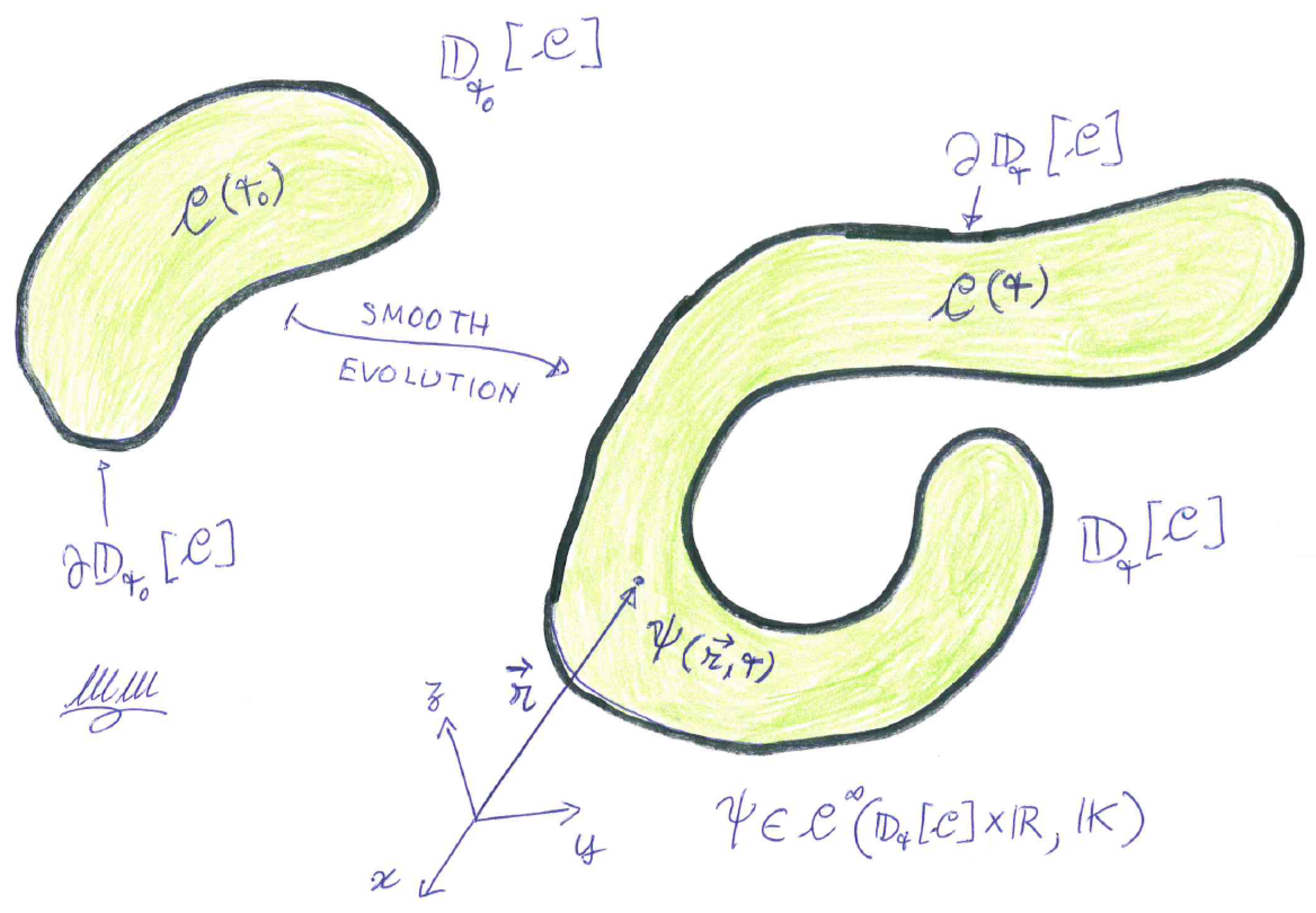
Figure 2.
A sketch of the “macroscopic infinitesimal”, i.e. “parcel”, of the continuum , containing a certain number of particles, indicated as red dots inside it, the centre-of-mass of which is the point P. The centre-of-mass velocity of all the particles within this is attributed to P as .
Figure 2.
A sketch of the “macroscopic infinitesimal”, i.e. “parcel”, of the continuum , containing a certain number of particles, indicated as red dots inside it, the centre-of-mass of which is the point P. The centre-of-mass velocity of all the particles within this is attributed to P as .
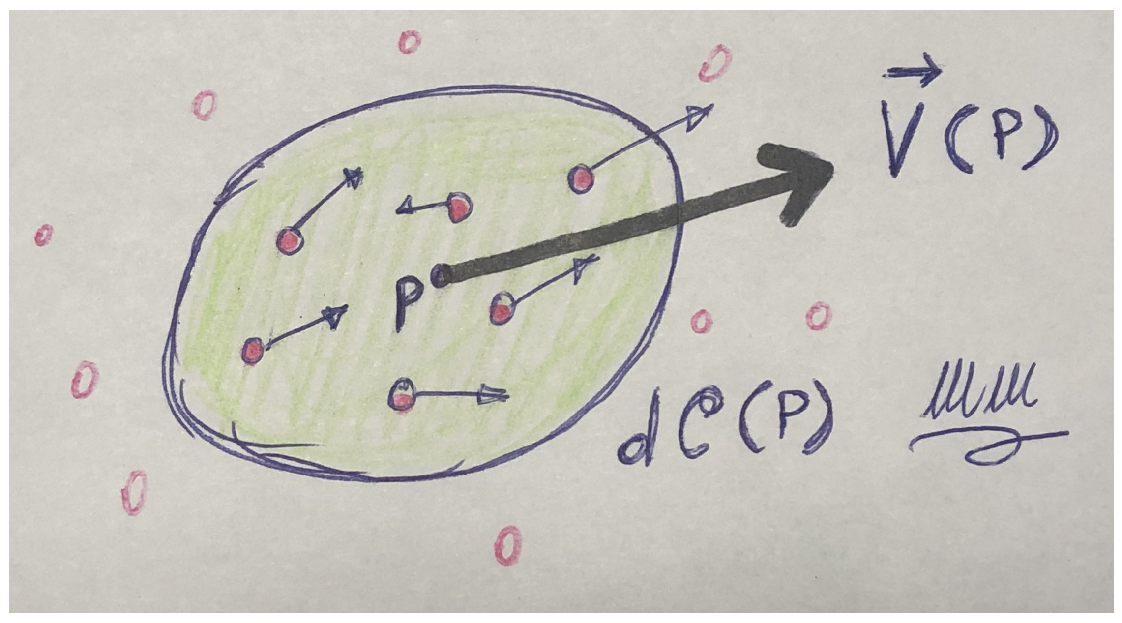
Figure 3.
The cartoon of how smoothness of macroscopic variables in FD should be intended: and are two “nearby” parcels, as the one portrayed in Figure 2, with centre-of-mass P and respectively, separated by a “small” displacement . and are respectively the “small” volumes of and .
Figure 3.
The cartoon of how smoothness of macroscopic variables in FD should be intended: and are two “nearby” parcels, as the one portrayed in Figure 2, with centre-of-mass P and respectively, separated by a “small” displacement . and are respectively the “small” volumes of and .
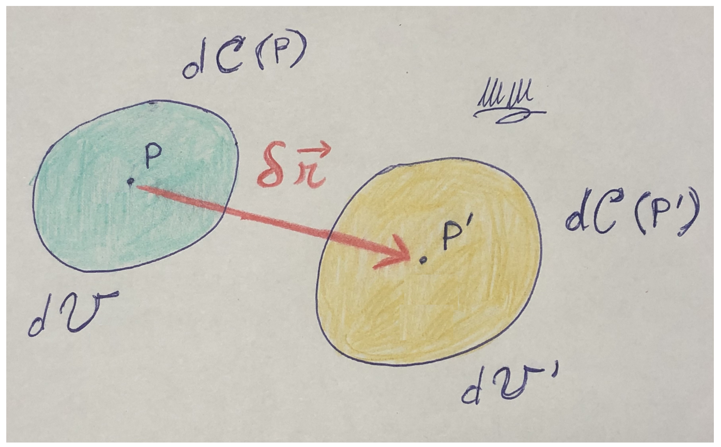
Figure 4.
The particles of the I-th species within the fluid parcel: the red dots represent the elementary components of the I-th species, while the red continuous line is the trajectory of as a whole.
Figure 4.
The particles of the I-th species within the fluid parcel: the red dots represent the elementary components of the I-th species, while the red continuous line is the trajectory of as a whole.
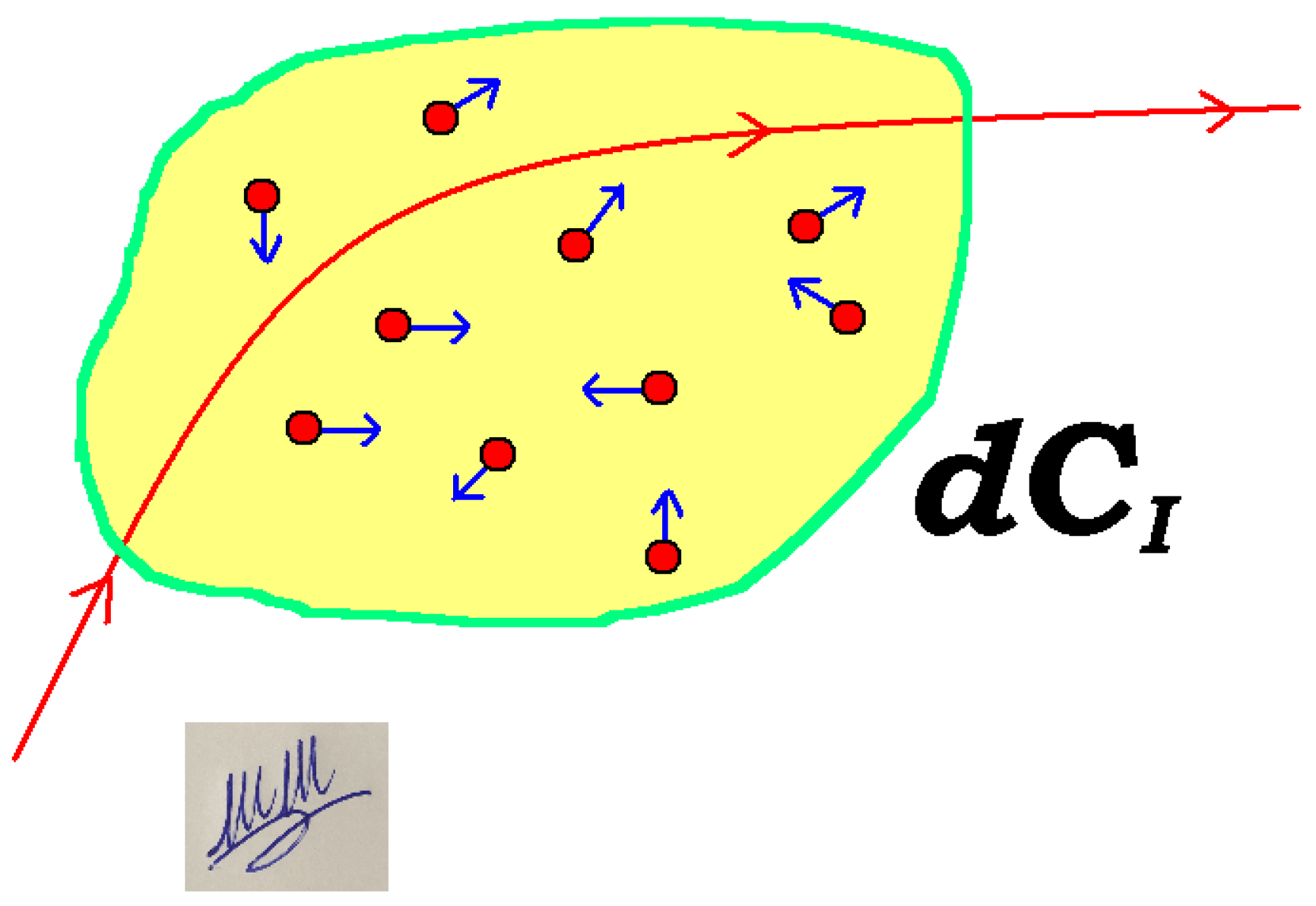
Figure 5.
The NeWReF versus the SERF: one defines the NeWReF through the transformations (180) and (183), then one puts the local Cartesian axes with z along , while the so-oriented NeWReF translates rigidly with respect to the SERF (without rotating). By the way, consider that the axes used in the transformations (184) and (185) are not the ones used in SubSection 4.2, where is parallel to and not to .
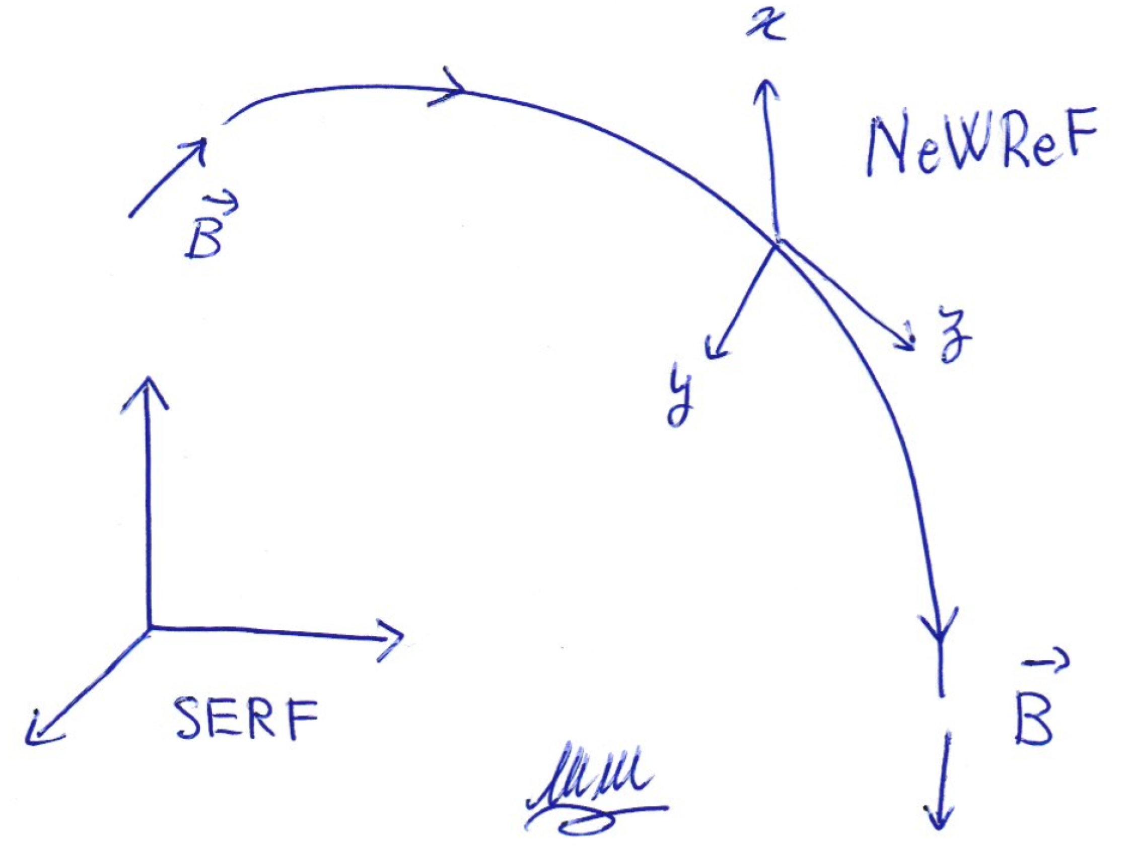
Figure 6.
Cartoon of a geomagnetic line of the field with the electrostatic ionospheric field : as the conductivity along is always much higher than that perpendicular to it in the ionosphere, at the electrostatic equilibrium vectors will lie perpendicularly to the lines of .
Figure 6.
Cartoon of a geomagnetic line of the field with the electrostatic ionospheric field : as the conductivity along is always much higher than that perpendicular to it in the ionosphere, at the electrostatic equilibrium vectors will lie perpendicularly to the lines of .
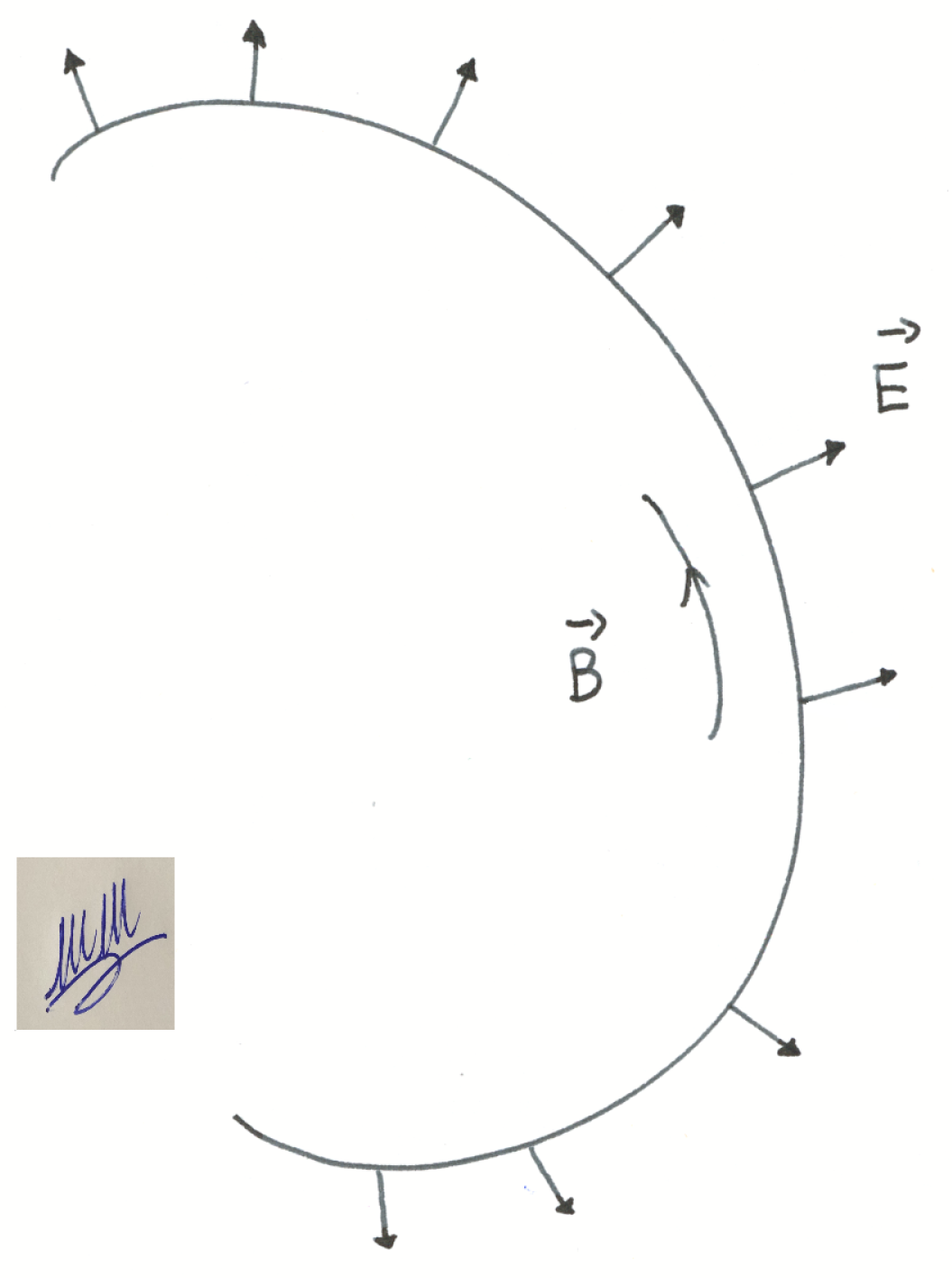
Figure 7.
Sketching the prevalent component of the geomagnetic field, which is dipolar, one sees that a point P of height h taken along the field line at high latitudes, dragged along the same field line down to low latitudes, will result in a corresponding position of bigger height .
Figure 7.
Sketching the prevalent component of the geomagnetic field, which is dipolar, one sees that a point P of height h taken along the field line at high latitudes, dragged along the same field line down to low latitudes, will result in a corresponding position of bigger height .
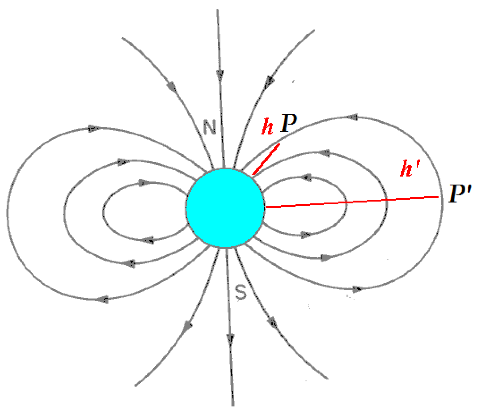
Figure 8.
Comparison between the “conservation” of wide electrostatic structures transported along a geomagnetic line from the Polar to the Equatorial Region, and the “dispersion” of small electrostatic structures, see the text.
Figure 8.
Comparison between the “conservation” of wide electrostatic structures transported along a geomagnetic line from the Polar to the Equatorial Region, and the “dispersion” of small electrostatic structures, see the text.
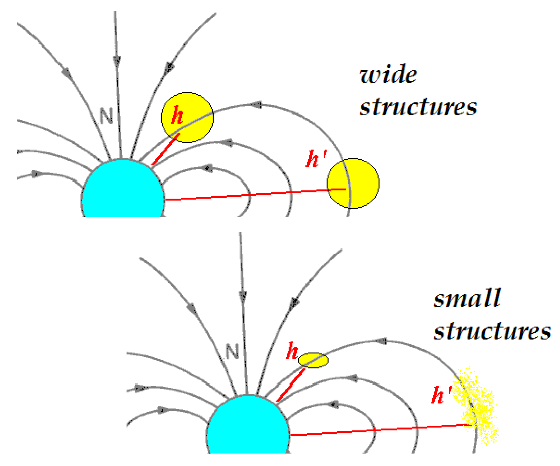
Figure 9.
The cartoon of the system described in SubSection 4.5.2, in which some electric current is injected along at high latitudes.
Figure 9.
The cartoon of the system described in SubSection 4.5.2, in which some electric current is injected along at high latitudes.
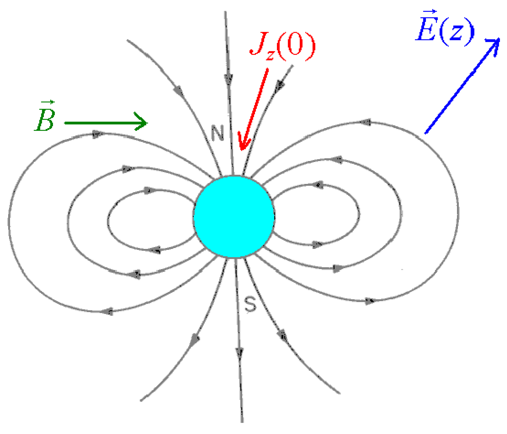
Disclaimer/Publisher’s Note: The statements, opinions and data contained in all publications are solely those of the individual author(s) and contributor(s) and not of MDPI and/or the editor(s). MDPI and/or the editor(s) disclaim responsibility for any injury to people or property resulting from any ideas, methods, instructions or products referred to in the content. |
© 2024 by the authors. Licensee MDPI, Basel, Switzerland. This article is an open access article distributed under the terms and conditions of the Creative Commons Attribution (CC BY) license (http://creativecommons.org/licenses/by/4.0/).
Copyright: This open access article is published under a Creative Commons CC BY 4.0 license, which permit the free download, distribution, and reuse, provided that the author and preprint are cited in any reuse.


