Abalone Age Prediction and Analysis of Influencing Factors: Combining Machine Learning, Shap and Correlation Coefficient Methods

1. Introduction

As a rare shellfish in the shallow sea, abalone has attracted much attention because its body is rich in a variety of active substances that have significant benefits to human health. In biology and fishery research, predicting the age of abalone not only helps to understand the life characteristics of abalone and formulate scientific aquaculture strategies, but also helps to analyze the growth rate and growth curves of abalone at different stages of growth, assess the population size and distribution, and provide important references for formulating biodiversity conservation strategies[1].

The traditional method of predicting the age of abalone is mainly to observe and analyze the growth rings of abalone shell. The abalone shell will leave a ring-like growth texture, like the annual rings of trees, as it grows. These rings show the growth history of the abalone. They are important for predicting the age of the abalone.[2]. The traditional observation method has some limits. It is especially hard to determine the age of young abalone or abalone with unclear growth rings. In addition, Algae and stains on the abalone shell can cover the growth rings. This makes it even harder to observe them. The growth rings are affected by different environmental factors. This causes some errors in the prediction results of traditional methods. [3].

Artificial intelligence technology is developing quickly. Now, different machine learning models are used to predict the age of abalone. Machine learning models can get features from data. This removes the limits of manual observation methods for abalone. Machine learning models are better than traditional methods. They can automatically find patterns in data. This makes predictions faster and more accurate. They can also handle complex problems and improve as more data is used.[4]. Machine learning methods are diverse and flexible. This lets us use different scenarios and model strengths to create more accurate and strong prediction systems. In the abalone age prediction task, common features include shell length, shell height, and weight. These features are usually linked to the age of the abalone. Machine learning models can find the complex relationship between these features and age using a lot of data. This helps predict the abalone's age accurately.

The goal of this study is to build an accurate and efficient age prediction model. It will use historical morphological data of abalone and machine learning methods. Firstly, the age of abalone was predicted quickly by combining different machine learning models. This went beyond traditional biological measurements and improved prediction accuracy. Secondly, the SHAP method was used in a new way to make the model easier to understand. It showed how each feature contributed to the prediction results. This improved the model's transparency and trustworthiness. Finally, feature correlation analysis was used to study the main factors that affect abalone age prediction. The feature selection process was improved to make the model stronger. Combining these innovations, this study provides a data-driven, interpretable and efficient solution for abalone age prediction, which has important theoretical and practical implications.

2. Dataset and Modeling Methods

In this study, a modular approach was adopted, and three modules were designed, namely: machine learning module, model validation module and model interpretation module. The machine learning module develops models using six machine learning methods. Model Validation Module The model validation module uses multivariate validation methods to assess model performance. The model interpretation module uses SHAP and correlation coefficient methods to interpret the optimal model. Figure 1 illustrates the entire research process including inclusion and exclusion criteria, feature selection, data segmentation, data balancing, model development and validation, model comparison, and optimal model selection and interpretation. Data preprocessing, machine learning model implementation, and model interpretation are implemented in Python using scikit-learn.

2.1. Dataset Description

The study for this experiment was taken from Population Biology of ” The Population Biology of Abalone (Haliotis species) in Tasmania” by Nash et al[5]. It contains information data on 4177 abalone. The dataset contains 9 features and the contents of the dataset are shown in Table 1.

2.2 Data Preprocessing

Based on the relationship between the age of the abalone and the number of rings, a column named “Age” was added using Equation (1) to derive the actual age of each abalone[6].

$$Age=Rings+1.5$$

(1)

Abalone growth is affected by complex factors, so we used interquartile spacing to describe the age-distribution relationship of abalone. Interquartile range (IQR) is a statistic that shows the spread between quartiles in a data set. It is used to measure how spread out the data is. It represents the difference between the upper quartile (Q3) and the lower quartile (Q1)[7]. The traditional 1.5-fold IQR does not always fit abalone growth patterns. So, the 2-fold IQR was used as the treatment threshold for outliers in this study. In the study, data with a 2-fold IQR were used as the threshold. Data greater than or less than 2-fold IQR were excluded as outliers[8]. Finally, 4014 data were collected.

In machine learning models, numerical data is often used for incoming predictions. A character type feature named “gender” exists in the dataset, so “gender” is numericized and a one-hot encoding method is used to encode the values of three different columns of “gender” (M, F and I) were encoded as three separate columns, where only one column had a value of 1 and the rest had a value of 0[9]. In the study, an effective numerical transformation was performed on the “gender” column and a gender feature was removed to avoid the problem of multicollinearity due to the high correlation between the dummy variables. In this way, the model is better able to handle the feature category of gender, thus improving the prediction performance.

These preprocessing steps ensure data quality and provide clean, efficient data to support subsequent model training and prediction.

2.3. Model and Feature Selection

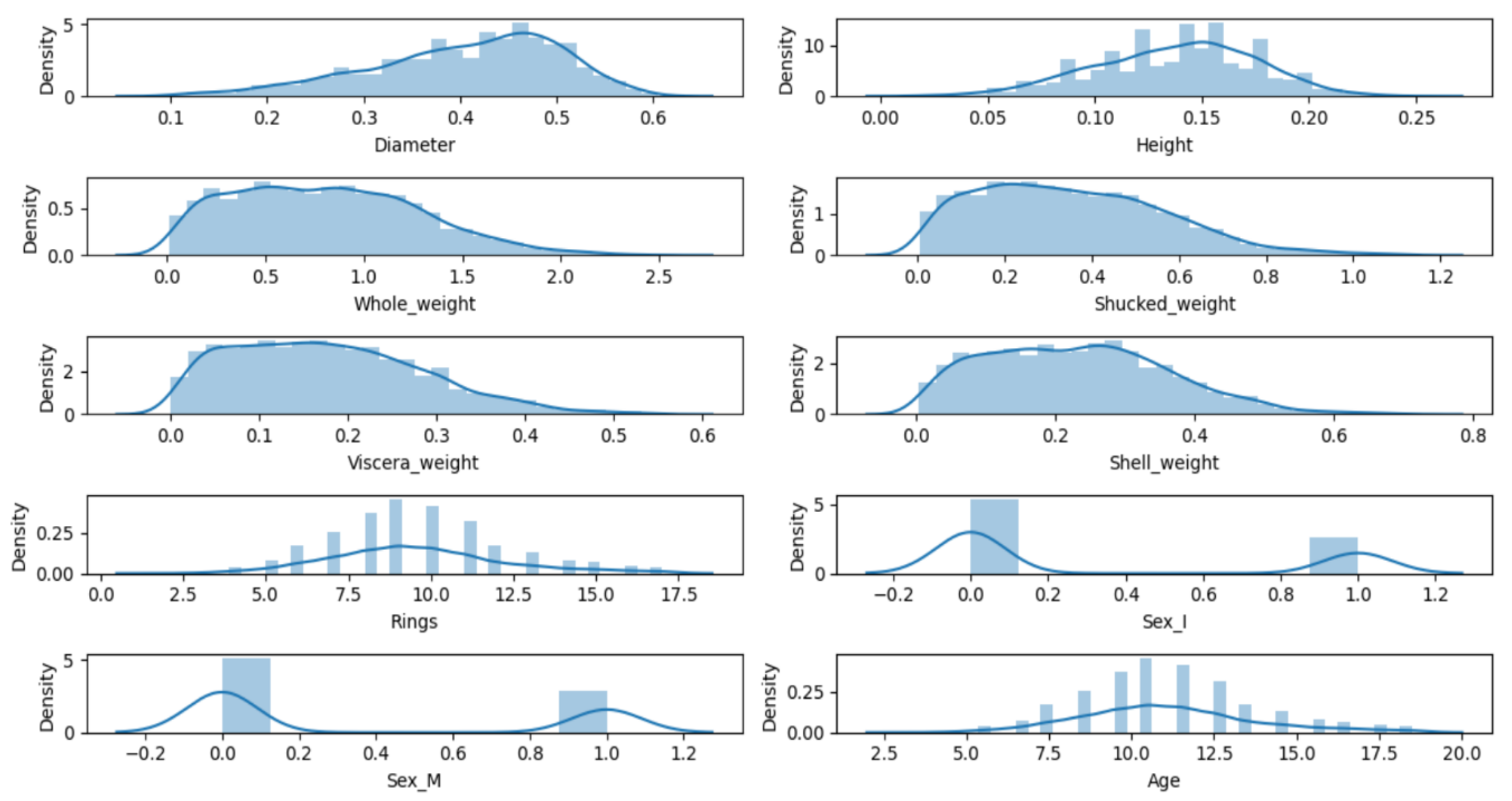
The histogram of the distribution of all data features in the dataset is shown in Figure 1. From Fig. 1, it can be analyzed that our data should have a linear relationship and at the same time may satisfy the normal distribution. In this study, six machine learning models that are widely used in biology research, i.e., Decision Tree (DT), Logistic Regression (LR), Random Forest (RF), Support Vector Machine (SVM), Extreme Gradient Boosting (XGBoost), and Adaptive Boosting (AdaBoost) are selected and combined with a 5-fold cross-validation, to compare MAE of these six machine learning models on the same data, RMSE and MAPE to determine an optimal model and obtain the feature importance of this optimal model for analysis[10].

Because the dimensionality of the data was not very large, no active culling of feature selection was performed in the study. There is a strong correlation between age and number of annual rounds of abalone, and equation (1) shows the proportionality between them. Therefore, “Age” and “Rings” were not selected as input features for the model. There are two reasons for this. Firstly, if the study had introduced “Rings” in the linear regression model, it would have significantly improved the accuracy of the model (up to 99% after testing the introduction of the number of rings). Secondly, if some of the features of the model already included “Rings”, this would mean that we already know the number of rings per abalone. In this case, there is no need to predict the age and the age of the abalone can be calculated using equation (1).

2.4. Dataset Segmentation

A common problem that arises in machine learning is the tendency of the chosen model to overfit. Such models overfit the test data but underfit the new data and do not generalize well. To address this problem, the data in the experiments were divided into a training set: test set with a ratio of 8:2, while the random seed was set to 42 to make it easier to reproduce the results of the experiments while ensuring the stability of the experimental sample.

3. Model Design and Evaluation

3.1. Model Design

The study used six machine learning models to test the test set data, including linear regression model (RL), decision tree (DT), random forest (RF), support vector machine (SVM), extreme gradient boosting (XGBoost), and adaptive boosting (AdaBoost)[10].

3.2. Model Evaluation and Optimization

Firstly, the prediction of the data with these six models is done directly using the default parameters and the test results obtained are shown in Table 2. The hyperparameters of these models were optimized using the grid-tuned parameter method and the 5-fold cross-validation method. Table 3 shows the hyperparameters and the final parameters for each tested model. Since abalone age prediction models do not need to be overly sensitive to errors, the MAE, RMSE and MAPE values were chosen as the evaluation criteria for the models in this study to assess the predictive ability of each model on the test set. In addition, the time complexity and model predictive ability of each model were evaluated to select the most suitable model for abalone age prediction and analyze it with an in-depth study.

Linear regression is a basic regression model that fits data by least squares. Its performance is relatively stable, but may not be as good as other complex models in some cases[11]. Its MAE and RMSE values are in the middle of the range. This means the model fits the data well, but it may have some bias in certain applications.

The decision tree model is easy to understand. It can segment the data based on its characteristics, but it is likely to overfit[12]. In terms of MAE and RMSE, it performs a little worse than linear regression. This suggests that, even though it captures some data patterns, the fit is not as stable as linear regression.

Random forest is a strong learning method. It makes the final prediction by building many decision trees and voting on them. Random forest can reduce overfitting and make predictions more stable compared to decision trees[13]. In this problem, Random Forest performs better in MAE and RMSE. This shows it can provide accurate and stable predictions.

SVM is a regression method based on boundaries. It handles complex nonlinear relationships well[14]. The MAE and RMSE of SVM are better than those of decision trees and linear regression. This shows it gives more accurate predictions. SVM takes longer to train. It is also more sensitive to data size and parameter settings.

XGBoost is an improved gradient boosting tree model. It is used in many machine learning problems. XGBoost improves the model step by step by adding weak learners. It works well with large and complex datasets[15]. In this study, XGBoost gives a balanced solution. It has good accuracy and stability.

AdaBoost is a comprehensive learning method that improves prediction accuracy by combining multiple weak learners[16]. Although AdaBoost can achieve good results on some problems, in this study, the MAE and RMSE results of AdaBoost are poor, which indicates that the model has weak generalization ability when dealing with this dataset.

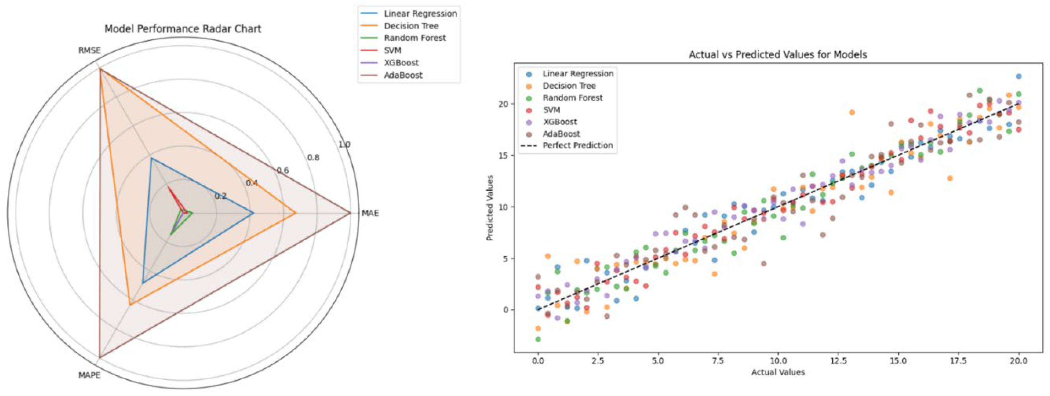
The results of the model evaluation after tuning are shown in Table 2. The evaluation results and prediction results of each model in the experiment are shown in Figure 2. From Figure 2, it can be found that SVM and XGBoost are two better models, especially in terms of MAE and RMSE, which are obviously better than other models. XGBoost and SVM both provide lower MAE and RMSE for the dataset, especially when dealing with complex data, which can better capture the nonlinear laws; XGBoost shows higher parameter tuning in terms of and high flexibility in parameter tuning, and the performance of the model can be improved by adjusting various parameters. Comparatively speaking, although Decision Tree and AdaBoost also have certain performance, the errors (e.g., MAE and RMSE) are larger, MAE and RMSE) are larger due to poor overfitting or generalization when dealing with this kind of problem.

Considering the accuracy, stability and applicability of the model, XGBoost is considered the best model. After literature search, it was found that the classical MAE for abalone age prediction in this study had an error of 1.8-2.0[3]. From the experimental results, it can be seen that XGBoost not only has a smaller error, with its MAE (1.3595) and RMS (1.8290) being 28.5% lower than the average of the classical MAE, but it also has a good tunability and flexibility, which makes it suitable for complex regression problems. However, its higher parameter sensitivity requires more tuning in practical applications, and it takes more time to train the SVM model, making XGBoost more advantageous.

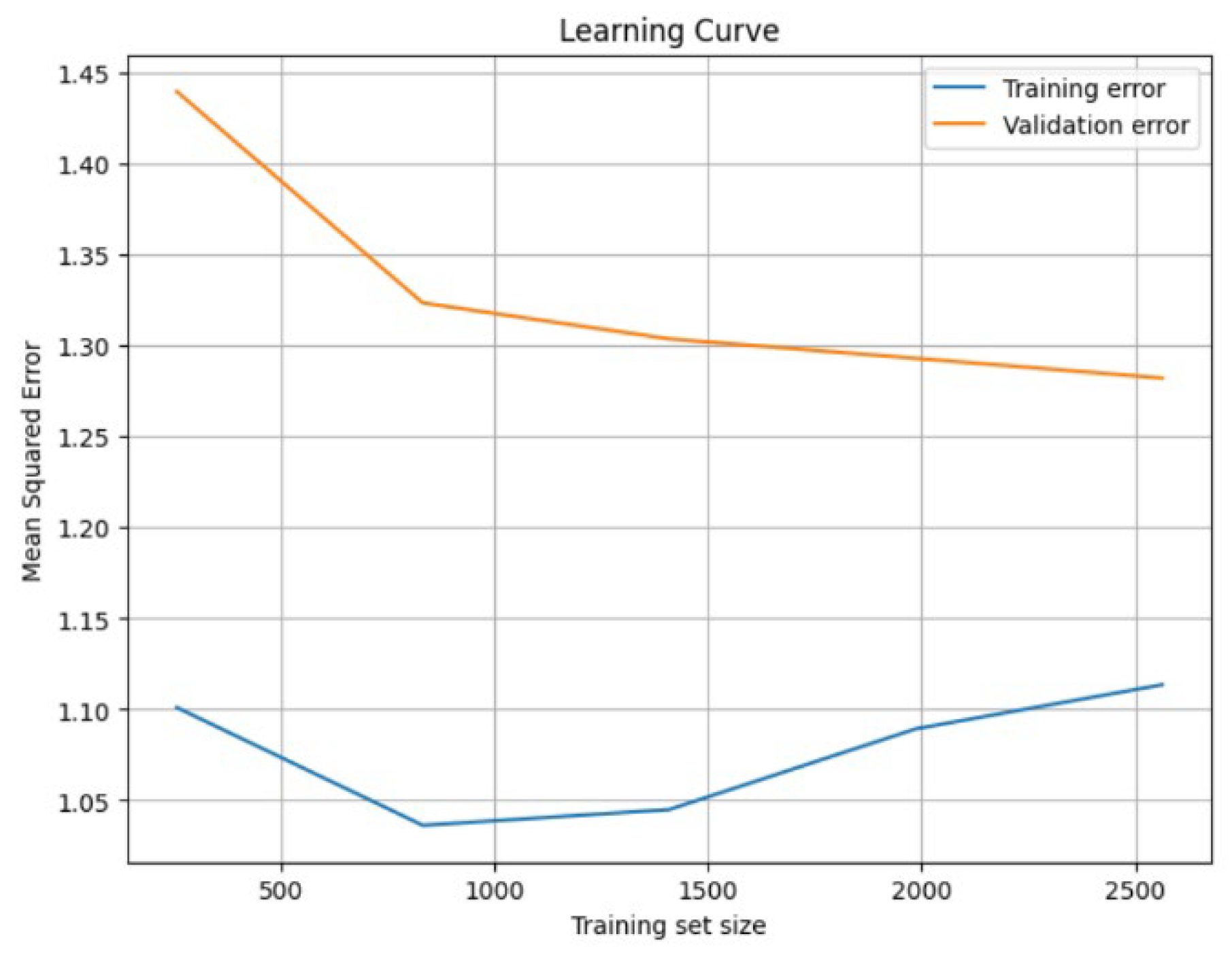
In order to validate the soundness of the XGBoost model in the field of machine learning, we studied the learning curve of the XGBoost model on these data, and the learning curve is shown in Figure 3. In the middle stage of model training, with the increase of training data, the model starts to have difficulty in fitting all data completely and the training error increases, but with the increase of training data, the generalization ability of the model improves, and the validation error starts to decrease significantly. In the late stage of the XGBoost model, the training error tends to stabilize and no longer increases significantly after reaching a certain error level, while the validation error gradually increases. At the same time, the validation error gradually decreases, but the magnitude of change becomes smaller, close to the training error. This indicates that the model has obtained a better generalization ability at this time, but there may be a slight bias. Therefore, the subsequent experiments will be analyzed based on the XGBoost model.

3.3. Feature Importance and SHAP Additivity Analysis

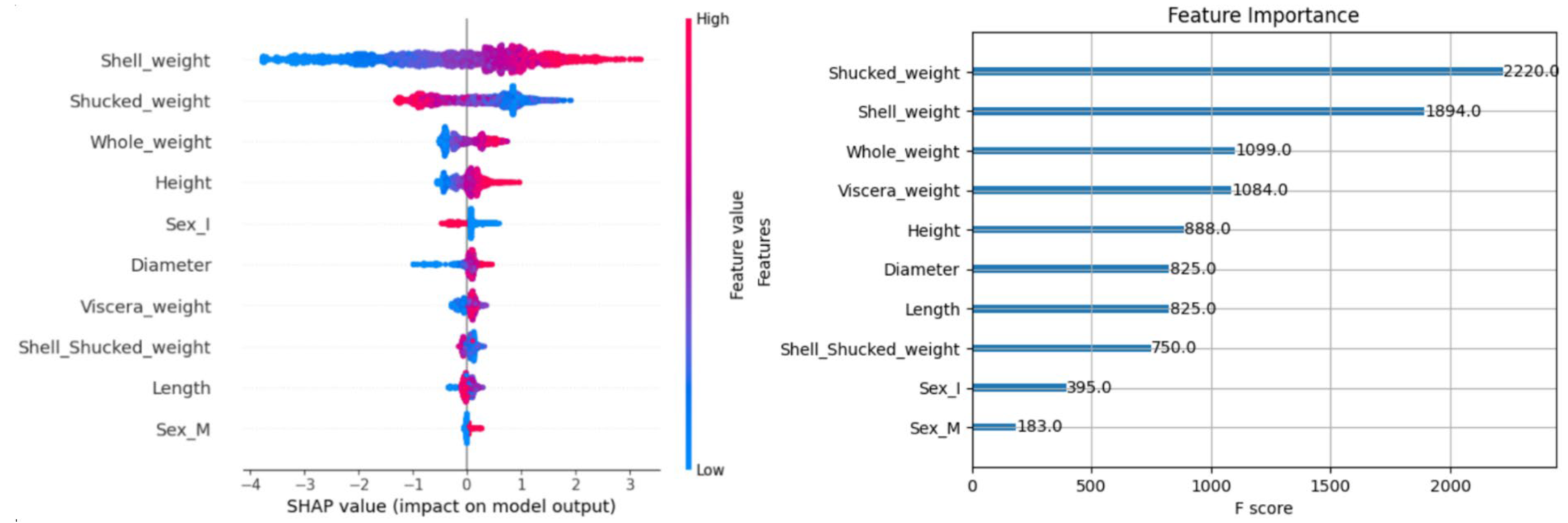
In order to analyze the feature importance of the XGBoost model, we plotted the feature importance map and SHAP analysis map based on the XGBoost model, as shown in Figure 4, respectively.

Feature importance plots are plots based on the importance of features, showing the importance scores of features, with each feature's score calculated based on the number of times the feature is used in the model[17]. SHAP plots are ranked based on the overall impact of the feature on the model predictions, with the impact of the feature increasing from the bottom to the top. The features with the greatest impact are at the top, and the horizontal SHAP value indicates the magnitude of the feature's contribution to the model output, with positive values indicating a positive correlation with the model output and negative values indicating an inverse correlation[18]. Each point indicates the feature value of the data sample and the magnitude of its contribution to the model output, and the color indicates the magnitude of the feature value.

According to Figure 4, the “Shucked_weight” feature has the highest importance with an F-score of 2220, but in the SHAP summary mapping, “Shell_weight” is ranked first and “Shucked_weight” is ranked second. This may be because feature importance mapping is based on segmentation frequency statistics, while SHAP summary mapping synthesizes the specific contribution of features to the prediction. Features with high segmentation frequencies do not necessarily have the greatest impact on the prediction results; for example, the gain may be small. In the SHAP maps, features are ranked in descending order of importance, with “Shell_weight”, “Shucked_weight”, and “Whole_weight” being the main drivers, and gender features such as “Sex_M” and “Sex_I” contributing less to model predictions, and subsequent research should focus more on “Shell_weight”, “Shucked_weight”, and “Whole_weight”. weight and “Whole_weight”. The degree of importance is based on the width of the distribution of feature SHAP values, the wider the distribution, the greater the influence of the feature on the model output[19]. the distribution of “Shell_weight” indicates that the higher the value of the feature, the higher the corresponding SHAP value. When the feature value is low, the SHAP value is mostly negative. Meanwhile, the distributions of some features show obvious non-linear relationships, such as height and diameter, whose SHAP values show obvious bimodal or heterogeneous distributions, which may mean that there are interactions between these features.

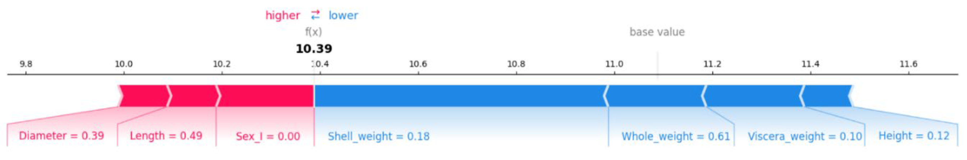
In order to investigate the specific effect of the eigenvalues on the contribution of the model and to improve the interpretability of the model, we plotted the interpretation of the SHAP values as shown in Figure 5, from which it can be seen that the red part “Diameter” pushed the predicted value by 0.39, indicating that a larger shell diameter of abalone is a significant factor in predicting an increase in the age of the abalone. “Length” pushed the predicted value by 0.49, indicating that a larger shell length of abalone also has a significant positive effect on the predicted age. Length drives the predicted value up by 0.49, indicating that the larger shell length of abalone also has a significant positive effect on the predicted age. “Sex_I” is 0, indicating that this trait contributes almost nothing, suggesting that sex has a small effect on the predicted age. “Shell_weight” drives the predicted value down by 0.18, indicating that the smaller shell weight of abalone has a somewhat negative effect on the predicted age. “Whole_weight” decreased by 0.61, indicating that the overall weight of abalone is lighter, which significantly reduces the predicted age. “Viscera_weight” decreased by 0.10, indicating that the viscera of abalone are lighter, which has a negative effect on the predicted age. “Height” decreased by 0.12, indicating that the height of abalone has a small negative contribution to the predicted age. So it means that “Diameter” and “Length” have the largest contribution, indicating that a larger diameter and length of the shell has a significant positive effect on the predicted age of the abalone, which is in line with the reality because the size of the shell may be closely related to the growth cycle of the abalone. “Whole_weight” is the feature with the largest negative contribution, indicating that the lighter overall weight significantly reduces the predicted age of the abalone. “Shell_weight” and “Viscera_weight” also had some negative contribution, indicating lower shell weight and viscera weight.

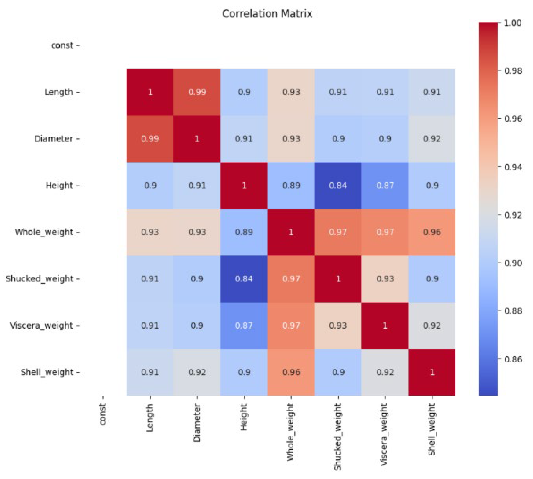
At the same time, according to the Pearson correlation coefficient method, correlation coefficients were plotted in the study, as shown in Figure 6. The red color indicates that the correlation between the variables is strong, and the blue color indicates that the correlation between the variables is weak or close to 0. The closer the color is to the red color, the stronger the linear positive correlation between the variables is; and the closer the color is to the blue color, the weaker the correlation between the variables is[20]. Therefore, according to the correlation coefficient graph, we can conclude that “Length” and “Diameter” (0.99): the length and diameter of the shell are highly positively correlated, indicating that the overall shape of the abalone is relatively regular, and that the length and diameter change synchronously with the size of the individual, suggesting that the length-to-width ratio of the abalone is relatively stable among different individuals and that the overall shape of the abalone is regular. And the specific analysis is as follows:

“Whole_weight” and “Shucked_weight”(0.97): The high correlation between “Whole_weight” and “Shucked_weight” suggests that the weight of shucked abalone is largely proportional to the overall weight. At the same time, the high correlation between “Length” and “Diameter” indicated that the length-to-width ratio of abalone was stable among individuals and the overall shape was regular, and the medium-to-high correlation between “Height” and “Diameter” indicated that the height was affected by the diameter to a certain extent, but the shapes of abalone might have slight differences.

“Whole_weight” and “Viscera_weight”(0.97): the total weight and “Viscera_weight” were highly positively correlated, indicating that the “Viscera_weight” of abalone was consistent with the trend of the overall weight.

“Shucked_weight” and “Viscera_weight”(0.93): the correlation between “Shucked_weight” and “Viscera_weight” is strong, probably because “Viscera_weight” is one of the main components of weight after shucking.

There is no significant negative correlation in the graph, indicating a positive linear relationship between all variables.

4. Model Application and Discussion

4.1. Biological Discussion

4.1.1. SHAP Additivity Analysis

“Shell_weight” had the widest distribution of SHAP values (-4 to 3), suggesting that it is the most influential and stable characteristic for age prediction in abalone. shell weight is related to mineral deposition (e.g., degree of calcification) as a natural consequence of long-term abalone growth. These findings help biologists to estimate the level of abalone growth and development from shell weight and to explore the mechanisms of shell mineralization. Meanwhile, abalone shells gradually gain weight during the growth process, and thus we believe that shell weight is an important indicator for assessing the growth cycle and maturity of abalone.

SHAP values for shucked weight and whole weight were also higher, suggesting that they contribute significantly to the age prediction of abalone. The distribution characteristics of both were like those of shell weight, and abalone with higher weights were usually older. The weight of abalone was closely related to the weight of muscle tissue and internal organs, and the shucked weight and whole weight increased significantly with age and more mature development of individuals. Shelling weight and overall weight reflect the nutrient accumulation and growth rate of abalone.

The SHAP value of “Viscera_weight” is moderate, indicating that viscera weight contributes to the age of abalone. “Viscera_weight” is another important indicator of nutrient accumulation in abalone, reflecting the health status and growth level of individuals[21]. The contribution of viscera weight to the prediction of abalone age mainly comes from the development and weight increase of viscera during the maturation process of individuals.

4.1.2. Correlation Coefficient Analysis

The correlation coefficient between “Length” and “Diameter” is 0.99, which is close to perfect positive correlation. The correlation coefficient between “Length” and “Height” was 0.90, and that between “Diameter” and “Height” was 0.91. These high correlation coefficients indicate that the shells of abalone in different sizes showed a tendency to synchronize with individual growth. The morphological development of abalone is regular, and the overall morphological proportions are relatively stable, which is in line with the natural growth pattern of organisms[22]. These results can help biologists to understand the dynamic changes of abalone shell morphology and provide data support for subsequent abalone morphology studies.

The correlation coefficient between “Whole_weight” and “Shucked_weight” is 0.97, the correlation coefficient between “Whole_weight” and “Viscera_weight” is 0.97, the correlation coefficient between “Whole_weight” and “Shell_weight” is 0.96, which show that the whole weight of abalone was highly correlated with shell weight, viscera weight and shucked weight, indicating a consistent growth trend in the body weight composition of abalone. These indicators can show abalone health, growth rate, and nutrient accumulation. They can help explore the developmental features of abalone at different growth stages[23].

4.2. Business Discussion

4.2.1. SHAP Additivity Analysis

"Shell_weight", "Shucked_weight", and "Whole_weight" are the main predictors of abalone age. These weight characteristics are directly connected to the market price of abalone. Abalone with higher shell and meat weights usually have a higher market value. Predicting the age of abalone with the model can help farmers choose the best time to harvest and make the most profit. Abalone with high shell and meat weights can be sold to the high-end market, and if a batch of abalone has low shell and shucking weights, it may be necessary to extend the culture cycle or adjust the feeding strategy[24].

“Length”, “Diameter”, “Height” and “Viscera_weight” reflect the growth and development of abalone. By monitoring the changes in shell length, shell width and “Viscera_weight”, the health status of abalone can be assessed at different growth stages. Individuals with slow growth or abnormal development can be identified to optimize culture density and resource allocation and reduce resource waste. Use SHAP model results to help farms make data-driven management decisions, e.g., identify high-value individuals (heavier, older abalone). Improve culture efficiency, shorten culture cycles, and reduce feed and labor costs.

Combined with the prediction model, abalone will be automatically categorized based on shell weight, meat weight, body size and other characteristics to achieve accurate pricing. For example, abalone with high meat weight can be categorized as high-end market products, while abalone with low shell weight can continue to be farmed. Meanwhile, through age prediction and growth characterization, the maturity time of different batches of abalone can be accurately predicted to optimize harvesting and supply planning. It improves the efficiency of the supply chain and ensures stable market supply[25].

4.2.2. Correlation Coefficient Analysis

The high correlation between “Viscera_weight” and “Whole_weight” indicates that the health of abalone can be monitored by viscera weight. If the viscera weight does not match other indicators, it may indicate health problems or abnormal growth of the abalone. By monitoring the relationship between viscera weight and total weight, farms can quickly screen out slow-growing and abnormal health of individual abalone and adjust the feeding strategy and water quality management in time to optimize the culture results[23].

The high correlation between abalone shell size and weight can provide a scientific basis for abalone selection and breeding. Individuals with a good ratio of shell weight to meat weight are chosen for genetic improvement. This helps increase the growth rate and yield quality of abalone. By tracking these indexes over time, new abalone varieties with strong adaptability and fast growth can be bred. This can improve the economic benefits and competitiveness of abalone farming.[24].

5. Summary and Outlook

This study focuses on the problems of traditional methods in abalone age prediction. It proposes a machine learning model for predicting abalone age. The method combines the SHAP algorithm and feature correlation coefficient analysis. By analyzing multiple features, the machine learning model can get useful information from complex linear relationships. This improves the accuracy of abalone age prediction. The SHAP algorithm helps the model give accurate predictions. It also shows how much each feature contributes to the prediction results. This makes the important factors in abalone age prediction clearer. At the same time, the correlation coefficient analysis helps find the linear relationship between features. This improves feature selection and makes the prediction model more stable and reliable. The experimental results show that the machine learning model is better than traditional methods for abalone age prediction. This is especially true when working with large-scale sample data, as it has better generalization and a lower error rate. However, the current model is still limited to the selected feature set, and its adaptability to environmental changes needs to be further verified[26]. In future studies, we will introduce more environmental factor variables, such as water temperature, salinity and current, to further improve the prediction accuracy and conduct corresponding experiments on other datasets.

References

- Jiao, Y., Rogers-Bennett, L., Taniguchi, I., Butler, J., & Crone, P., 2010. Incorporating temporal variation in the growth of red abalone (Haliotis rufescens) using hierarchical Bayesian growth models. Canadian Journal of Fisheries and Aquatic Sciences, 67, pp. 730-742. [CrossRef]
- Yoneyama, S., 1991. Formation of Shell Growth Rings in the Abalone, Haliotis gigantea from Izu-Oshima., 39, pp. 181-188. [CrossRef]
- Geibel, J., Demartini, J., Haaker, P., & Karpov, K., 2010. Growth of Red Abalone, Haliotis rufescens (Swainson), Along the North Coast of California., 29, pp. 441 - 448. [CrossRef]
- Grebovic, M., Filipović, L., Katnic, I., Vukotić, M., & Popović, T., 2023. Machine learning models for statistical analysis. Int. Arab J. Inf. Technol., 20, pp. 505-514. [CrossRef]
- UCI Machine Learning Repository, Abalone dataset. https://archive.ics.uci.edu/ml/datasets/Abalone.
- Rodhouse, P.G., Hatfield, E.M.C., 1990. Age determination in squid using statolith growth increments. Fisheries Research 8, 323–334. [CrossRef]
- Whaley, D., 2005. The Interquartile Range: Theory and Estimation.
- Massara, P., Bandsma, R., Bourdon, C., Maguire, J., Comelli, E., Birken, C., & Keown-Stoneman, C., 2020. Outlier Detection in Growth Data: Beyond Biologically Implausible Values. Current Developments in Nutrition. [CrossRef]
- Alaya, M., Bussy, S., Gaiffas, S., & Guilloux, A., 2017. Binarsity: a penalization for one-hot encoded features in linear supervised learning. J. Mach. Learn. Res., 20, pp. 118:1-118:34.
- Liu, L., Bi, B., Cao, L., Gui, M., Ju, F., 2024. Predictive model and risk analysis for peripheral vascular disease in type 2 diabetes mellitus patients using machine learning and shapley additive explanation. Frontiers in Endocrinology 15. [CrossRef]
- Hussin, A., Abdullah, N., & Mohamed, I., 2010. A Complex Linear Regression Model.
- Vandewiele, G., Lannoye, K., Janssens, O., Ongenae, F., Turck, F., & Hoecke, S., 2017. A Genetic Algorithm for Interpretable Model Extraction from Decision Tree Ensembles., pp. 104-115. [CrossRef]
- Talekar, B., 2020. A Detailed Review on Decision Tree and Random Forest. Bioscience Biotechnology Research Communications. [CrossRef]
- Huoli, W., 2005. SVM Nonlinear Regression Algorithm. Computer Engineering.
- Fatima, S., Hussain, A., Amir, S., Ahmed, S., & Aslam, S., 2023. XGBoost and Random Forest Algorithms: An in Depth Analysis. Pakistan Journal of Scientific Research. [CrossRef]
- Gao, C., Sang, N., & Tang, Q., 2010. On selection and combination of weak learners in AdaBoost. Pattern Recognit. Lett., 31, pp. 991-1001. [CrossRef]
- Greenwell, B., & Boehmke, B., 2020. Variable Importance Plots - An Introduction to the vip Package. R J., 12, pp. 343. [CrossRef]
- Ponce-Bobadilla, A., Schmitt, V., Maier, C., Mensing, S., & Stodtmann, S., 2024. Practical guide to SHAP analysis: Explaining supervised machine learning model predictions in drug development.. Clinical and translational science, 17 11, pp. e70056. [CrossRef]
- Gebreyesus, Y., Dalton, D., De Chiara, D., Chinnici, M., & Chinnici, A., 2024. AI for Automating Data Center Operations: Model Explainability in the Data Centre Context Using Shapley Additive Explanations (SHAP). Electronics. [CrossRef]
- Gaddis, M., & Gaddis, G., 1990. Introduction to biostatistics: Part 6, Correlation and regression.. Annals of emergency medicine, 19 12, pp. 1462-8. [CrossRef]
- Chen, W., Meng, X., & Tao, P., 2004. Comparative studies on nutritional composition of abalone Haliotis discus hannai between two shell-color stocks. Journal of fishery sciences of China, 114, pp. 367-370.
- Worthington, D., Andrew, N., & Hamer, G., 2008. Covariation between growth and morphology suggests alternative size limits for the blacklip abalone, Haliotis rubra, in New South Wales, Australia.
- You, W., Ke, C., Luo, X., & Wang, D., 2010. Genetic Correlations to Morphological Traits of Small Abalone Haliotis diversicolor., 29, pp. 683 - 686. [CrossRef]
- Hossain, M., & Chowdhury, N., 2019. Econometric Ways to Estimate the Age and Price of Abalone.
- Huang, C., Vinh, N., Chen, Y., Liang, T., Nan, F., & Liu, P., 2019. Improving productivity management of commercial abalone Haliotis diversicolor supertexta and Haliotis discus hannai aquaculture in Taiwan: A bioeconomic analysis. Aquaculture. [CrossRef]
- Mccormick, T., Navas, G., Buckley, L., & Biggs, C., 2016. Effect of Temperature, Diet, Light, and Cultivation Density on Growth and Survival of Larval and Juvenile White Abalone Haliotis sorenseni (Bartsch, 1940). Journal of Shellfish Research, 35, pp. 981 - 992. [CrossRef]