
Submitted:
10 January 2025
Posted:
13 January 2025
Read the latest preprint version here
Abstract
The equation of time (EoT) tracks daily deviations in length between the solar day and the mean day. Since the length of the mean day remains constant throughout the year, the EoT must mirror daily fluctuations in the length of the solar day. Furthermore, if the Sun meridian declination (SMD) is dynamically linked to Earth’s rotational speed (ERS) the EoT must obey to oscillations in ERS. This document examines the position, velocity, acceleration, and net drive of the mean-time Sun within a solar sundial noon analemma considering both its vertical and horizontal dimensions: the SMD and the EoT. Evidence supports that ERS decreases monotonically along two trans-equinoctial analemmatic phases in which the net drives of the EoT and SMD become coordi-nated (either both accelerating or both decelerating) within the SMD interval of −16 to +19 arcdeg, centered at +3. Conversely, ERS increases monotonically along two trans-solstitial analemmatic phases in which the net drives of the EoT and SMD become opposed, outside the specified interval of SMD. The ERS reaches its minima and maxima at the troughs and crests of the EoT; whereas it varies respectively.
Keywords:
Earth’s rotational speed
; analemmatic dynamics
; natural beam irradiance
; length of the solar day
; equation of time
; solar sundial noon analemma
; Sun-Earth physics
1. Introduction
Despite the fluctuations in Earth’s rotational speed being recognized factual for timescales from daily to centennial, the prevailing theory attributes these variations primarily to the conservation of the angular momentum [1] overlooking the complexity of Sun-Earth physics. It is widely accepted that the dynamics of the Equation of Time (EoT) arise from the shape of Earth’s orbit and the tilt of Earth’s rotational axis [2,3]. However, the analemmatic dynamics of the Sun meridian declination (SMD) and the EoT remains underexplored. The analysis on these pages builds on a previous study that assessed the dynamics of the SMD to estimate the latitudinal budget of natural beam irradiance on Earth [4]. The current work evaluates the combined dynamics (velocity, acceleration, net drive, etc.) and synchrony between the SMD and the EoT within a solar noon analemma, aiming to establish a connection to Earth’s rotational speed (, km h−1) across daily, monthly, and seasonal timescales.
When the SMD is plotted against the EoT it yields the solar noon analemma, a lemniscate describing the combined horizontal-vertical path of the mean-time noon Sun along the Gregorian year, as perceived from a specific location on Earth’s surface [5]. Following the SMD within a solar noon analemma, the mean-time Sun travels from north to south and backwards, depicting the analemma‘s y-coordinate or the Sun’s vertical path. Following the EoT within the solar noon analemma the mean-time Sun travels from east to west and backwards, depicting the analemma‘s x-coordinate or the Sun’s horizontal path.
The EoT establishes a rhythm for the daily divergence between mean time and solar time, specifically between the lengths of the mean day and the solar day [6]. Consequently, if SMD is linked to the variation in Earth’s rotation along the planet’s orbit, then the EoT reflects not only fluctuations in the length of successive solar days but also variations in Earth’s rotational speed. This hypothesis might seem bold, but the Sun’s vertical path (SMD) and the Sun’s horizontal path (EoT or ) are synchronized in such a perfect harmony that evidence supports causal in lieu of casual connection.
If natural beam irradiance (NBI) is expected to align with the local meridian at mean time noon, but the EoT occurs to the left or right of the meridian, this deviation evidences a daily fluctuation in the length of the solar day and Earth’s rotational speed. This proposal assumes the Sun-Earth physics is inherently linked to Earth’s rotation, even challenging the role of angular moment as the primary driver of Earth’s rotational dynamics. Because the length of the solar day is tied to the Earth’s rotational speed [7], the light cone supplying NBI to the subsolar point [4] comprises the clock hand defining the only time frame Earth adheres to—the solar time. To comprehend the cause-effect relation between the EoT and the SMD, their interaction must be considered in isolation from any third factor. Earth does not revolve around distant stars nor adhere to civil time, the length of the day should neither be defined by distant stars, nor by a timeframe limited to 24 hours.
The inverse relationship between the length of the solar day and Earth’s rotational speed requires reversing the scale of the EoT for an intuitive analysis, as suggested in a previous study on fluctuations in the length of the planet’s sideral day [8]. The given inverse association motivated the analysis of the Sun’s horizontal path (EoT) within a solar sundial noon analemma. In this context, negative EoT values correspond to periods when the rotational speed falls below the annual average and the mean-time Sun lags behind its mean velocity. Conversely, positive EoT values correspond to periods when the rotational speed exceeds the annual average and the mean-time Sun runs ahead of its mean velocity. Following a sundial noon analemma, Earth’s rotational speed must increase as the EoT advances from left to right and decrease as it progresses from right to left. Within a solar sundial noon analemma, the mean-time Sun travels from left to right during each of two trans-solstitial analemmatic segments, and from right to left during each of two trans-equinoctial analemmatic segments.
2. Materials and Methods
To analyze the joint vertical-horizontal path of the mean-time Sun, let denote the SMD and the EoT (both in arcdeg). Therefore, the joint function displays the solar sundial noon analemma, which illustrates the bidimensional path of the mean-time noon Sun throughout a Gregorian year, because the sundial analemma tracks the shifts of the mean-time Sun concerning both the SMD and the EoT. The records of and correspond to the vertical and horizontal angles from the mean-time noon Sun to the Equator () or the local meridian (), respectively. The difference in lengths between the mean day and the solar day (EoT) can be expressed in a variety of units including time (min), distance (km), and spheric-coordinates (arcdeg). For the present analysis arcdeg was chosen, to match the units in which solar declination is usually stated. The EoT and the Sun’s horizontal-path () are referred to as synonyms in this document, while the same holds true for the SMD (true declination) and the Sun’s vertical-path ().
2.1. Parameters of the Sun’s Vertical Path
The SMD (, Equation (2)) was derived from the fractional year (Equation (1)) modified for solar noon, following the analemma’s geometric model [9]. Let denote the position of the Sun’s vertical path (SMD), which tracks the angular distance between the mean time Sun and the Equator throughout the year. To explore the dynamics of the Sun’s vertical path in greater depth, five additional parameters were analyzed: angular velocity (, arcmin day−1), angular acceleration (, arcsec day−2), angular jerk (, arcjerk day−3), angular snap (, arcsnap day−4), and net drive () of the SMD. The functions , , , and correspond to the first to fourth derivatives (Equations (3) to (6)) of SMD () with respect to time (), same order. The net drive (Equation (7)) is defined by the sign of the product , where is stated as accelerative (speeding up) when the sign is positive or decelerative (slowing down) when negative.
where is the fractional year (radians), is time within a year (days, 1 to 365).
2.2. Parameters of the Sun’s Horizontal Path
The EoT (, Equation (8)) was derived from the fractional year (Equation (1)) modified for solar noon, following the geometric model [9] of the analemma. Let denote the position of the Sun’s horizontal path (EoT) which tracks the angular distance between the mean time Sun and the local meridian throughout the year. To explore the dynamics of the Sun’s horizontal path in greater depth, five additional parameters were analyzed: angular velocity (, arcmin day−1), angular acceleration (, arcsec day−2), angular jerk (, arcjerk day−3), angular snap (, arcsnap day−4), and net drive () of the EoT (). The functions , , , and correspond to the first to fourth derivatives (Equations (9) to (12)) of the EoT with respect to time (), same order. The net drive (Equation (13)) is defined by the sign of the product , where is stated as accelerative (speeding up) when the sign of the given product is positive or as decelerative (slowing down) when negative.
where is the fractional year (radians, Equation (1), is the time within a year (days, 1 to 365). The minus sign of Equations (8) to (12) switch the EoT from an on-sky to a sundial noon analemma.
All signs of the horizontal path were arbitrarily reversed (Equations (8) to (12)) from those arising from the geometric model of solar declination, to produce the solar sundial noon analemma. Inverting the signs of the EoT allowed to intuitively associate negative records of to moments where the Sun travels slower on its daily path, yielding longer solar days. Likewise, positive records of correspond to moments where the Sun travels faster on its daily path, yielding shorter solar days. Despite the ordinate axis of the sundial analemma being also reversable, such inversion was inappropriate for the planned discussion.
2.3. Adequate Units for the Path of the Mean-Time Noon Sun
When defining appropriate units to express first the parameters of the Sun’s vertical path (, , , , and ; Equations (2) to (6), and later those of the Sun’s horizontal path (, , , , and ; Equations (8) to (12), the guiding fact was that every successive derivative shortened its range of occurrence by a factor of approximately radians (radians being the original unit), equivalent to arcdeg. Accordingly, the kth derivative of the Sun´s horizontal position shortened its range by. In order to avoid working with too small numbers, every parameter was scaled up by the factor, which is already included in Equations (2) to (6) and Equations (8) to (12). The k superscript corresponds to the derivative order, whether for or , which becomes zero for Equation (2) and Equation (8), whereas the +1 converts the units from radians to arcdeg.
After applying the factor, the numerical value of every successive derivative became scaled up by with respect to its integral; for instance, the fourth derivative was scaled by . Consequently, it was only natural to down scale the units for all the parameters [4]. The original unit was rad day−k, whereas the units proposed here for the position, velocity, acceleration, jerk, and snap are: arcdeg, arcmin day−1, arcsec day−2, arcjerk day−3, and arcsnap day−4, same order. After the factors were applied and the units assigned, the records of all the parameters of the SMD and the EoT fell within a similar range, which allows to display various parameters in a unique ordinate axis despite their differing units. Nonetheless, any comparison proposed between the parameters must refer their scales. In order to establish the similarities between the dynamics of the SMD () and that of the EoT () analogous symbols and identical units were proposed to refer equivalent parameter whether for the Sun’s vertical or horizontal path ( and , and , etc.).
When the positional parameters (and ) and their derivatives are plotted against time, they display pseudo sinusoidal functions. Consequently, the classic terminology of sinusoidal curves is adopted from this point onward. In this context, the time interval in which a full cycle is completed is known as the period. A cycle can be further divided into two half-cycles, each framed between two zero-crossing points (ZCPs) two crests, or two troughs. When the ZCPs of the position (and ) are chosen to divide a cycle into half-cycles, a crest occurs midway within a positive half-cycle, whereas a trough occurs midway within a negative half-cycle. Unlike the SMD and the EoT ( and ), the crests and troughs of actual sinusoidal are equidistant from their ZCPs (the abscissa), and such distance is referred to as the cycle’s amplitude. For practical purposes, the annual cycle of the Sun’s horizontal path was considered as a dual cycle —which is framed within a unique cycle of the Sun’s vertical path—, despite initial and final conditions of the EoT only converging by the end of the Gregorian year.
2.4. Sections of the EoT
The Sun’s vertical-path () was divided into two half-cycles by the ZCPs of , which converge at the equinoxes to either the crest or through of —where a trough corresponds to a crest when points downward and is negative—. Every half-cycle tracks the SMD within one hemisphere. Furthermore, dividing each half-cycle of the SMD by the solstitial ZCPs of , yielded quarter-cycles which frame an entire season. Furthermore, the Sun’s horizontal-path () was divided into two cycles by the two troughs of and every cycle divided in two half-cycles by the crests of . Finally, eight sections were produced by dividing every half-cycle into two sections by the ZCPs of . Every resulting section comprised whether the first or the last of the two quarter-cycles conforming a season. Because the division was conducted by the key instances of rather than by time ranges, the resulting sections differ in duration. T
The Sun’s vertical path () takes ZCPs at the Equator, whereas the Sun’s horizontal-path () takes ZCPs at the local meridian. To analyze the annual dual cycle of the Sun’s horizontal path, the EoT was divided in eight sections by the four maxima and four ZCPs of . The section boundaries can be either a crest and a ZCP of , or a ZCP and a trough of . Let the section names be early spring, late spring, early summer, late summer, early autumn, late autumn, early winter, and late winter. Let the section boundaries be denoted spring equinox, midspring, summer solstice, midsummer, autumn equinox, midautumn, winter solstice and midwinter.
To investigate the connection between the EoT and Earth’s rotation, the analemma was further divided into four phases: trans-equinoctial phases I and III and trans-solstitial phases II and IV. Each phase includes two consecutive sections of the EoT, while the numbers obey to the order in which they occur. Unlike the seasons of the SMD, which consist of two sections with opposing horizontal directions—the direction of the EoT—, each analemmatic phase consists of two consecutive sections whose horizontal direction is consistent both within and between. The direction of the EoT is identified by the sign of , where points right when the sign is positive or left when negative. Each analemmatic phase extends between two ZCPs of . The trans-equinoctial phase I occurs between the midwinter and midspring, and the trans-equinoctial phase III occurs between midsummer and midautumn. Therefore, the trans-equinoctial phase I encompasses late winter and early spring while the trans-equinoctial phase III includes late summer and early autumn. The trans-solstitial phase II occurs from midspring to midsummer and the trans-solstitial phase IV spans from midautumn to midwinter. Therefore, the trans-solstitial phase II encompasses late spring and early summer, while the trans-solstitial phase IV includes late autumn and early winter.
Each phase shows homogeneity regarding four aspects: (1) the sign of , and consequently (2) the direction of ; which inherits a consisting direction to both (3) Earth’s rotational speed and (4) to the length of the solar day. When only numerical data are available, the sign of is the sole indicator for the direction in which the Sun’s horizontal path occurs. The concept of phase within the EoT, was key for studying the dependance between the EoT, the length of the solar day, and Earth’s rotational speed.
2.5. Earth’s Rotational Speed and the EoT
Because the Earth orbits the Sun rather than the galaxy or distant stars, studies on Earth dynamics must prioritize Sun-Earth interactions. Given that Earth’s rotational speed () is discussed alongside the vertical () and horizontal () velocities of the mean-time noon Sun, the concept “speed” is reserved for the planet’s rotation. This is appropriate because the rotational speed is always positive.
This document defines solar day as the unique true day and assumes the Sun’s horizontal path is inherently tied to Earth’s rotation. On a hypothetical day when the EoT runs 16 min ahead of the meridian, this offset corresponds to a horizontal angle of +4 arcdeg beyond the local meridian, equivalent to 240 arcmin per day or 10 arcmin per hour compared to the mean day. This deviation indicates the Sun’s horizontal path extends 445 km above the mean day and the equatorial rotational speed is 18.5 km hour−1 faster than the annual average speed. The EoT , must be either added to or subtracted from the average speed of rotation (1669.78 km h−1). In fact, Earth’s rotational speed varies from 1653 to 1688 km h−1 at the Equator (or 27.5 to 28.1 km min−1). A fluctuation involving ±1 % throughout the year , equivalent to 852 km day−1, 35.5 km h−1, or 0.6 km min−1 between the maximum and minimum speeds.
Because Earth’s linear rotational speed varies with latitude, it is convenient to derive an expression which accounts for this factor. The linear regressions in Equations (15) and (16) establish the association between Earth’s rotational speed and the EoT, for the Equator and the Tropic of Cancer, respectively, both derived from Equation (14). A general formula for Earth’s speed of rotation is also given in Equation (17), which considered the following steps: (1) assesses Earth’s circumference (km) at the desired latitude , which is the distance the Sun’s horizontal path travels within a day, given by , (2) derive an equivalence between angular and linear distances by dividing Earth’s circumference by 360 arcdeg, (3) add the EoT to Earth’s circumference, both in km [10], and (4) dividing the outcome by the 24 hours of a mean day. The radius of Earth’s circumference and the Earth’s average speed were and .
where is the Earth’s rotational speed on day , is the site’s latitude and is the EoT on day .
3. Results and Discussion
3.1. The Signs Paradox
The signs of the parameters describing the Sun’s vertical path (, and ) arise because the Northern Hemisphere is the customary reference across science. Nonetheless, the signs can be reversed without semantic consequence, which would mean the Southern Hemisphere is the reference. Actually, the signs of SMD reverse naturally between hemispheres without interfering with the net drive of declination (speeding up or slowing down) of any season. Otherwise stated, the dynamics of the SMD would remain unaffected whether analyzed through austral or boreal seasons. Accordingly, whether a ZCP of occurs downward or upward is irrelevant from the standpoint of physics, which holds true for the ZCPs of . Hence, absolute values can be taken from , and when their association is assessed within hemisphere.
Unlike the signs of the parameters describing the Sun’s vertical path …), those of the horizontal path …) cannot be reversed without consequence. For the Sun’s horizontal path (), the meaning of a positive half-cycle opposes that of a negative half-cycle. The analyses undertaken in this work are based on a sundial meridional analemma, on which the direction of reverses from west to east and vice versa compared to a sky solar noon analemma. Reversing the signs is beneficial when relating the EoT to the Earth’s rotational speed or the length of the solar day. For instance, at the ZCPs of the EoT, the length of the solar day and Earth’s rotational speed converge to their annual averages (24 hours and 1669.78 km h−1). A ZCP of can occur both within a trans-equinoctial phase —where the rotational speed decreases progressively— and within a trans-solstitial phase —where the rotational speed is progressively increasing. Therefore, the former conforms a downward ZCP and the latter conforms an upward ZCP, which switch from positive to negative records or from negative to positive records, respectively.
Every time switches signs at a phase’s boundary (midseason ZCPs of ), Earth’s rotational speed switches between from a growing to a decreasing streak, or vice versa, while the dynamics of the length of the solar day reverses direction simultaneously, varying inversely with Earth’s rotational speed.
3.2. Dynamics of the Sun Meridian Declination
The within season averages for position (), angular velocity () acceleration (), jerk (), snap () and net drive () of the SMD are shown in Table 1. Given that the Sun meridian declination () defines the y-coordinate of the solar noon analemma as perceived from a given site on Earth’s surface, the annual cycle of SMD is referred through this document as the vertical path of the Sun (). The period of the Sun’s vertical-path () extents for one year, which can be split into a positive half-cycle that spans the Northern Hemisphere and a negative half-cycle that spans the Southern Hemisphere. The crest and trough of converge with the equinoxes, whereas the ZCPs of concur with the solstices.
The functions and approach circumference-like shapes. Accordingly, || and || vary inversely, so the highest || occurs at the lowest || and vice versa. An analogous association occurs between || and ||. Furthermore, || and || vary directly and approaches a straight line. The factor , included in Equations (3) to (6), was applied because each successive derivative of occurred within 1/60th of the range spanned by its integral when all the parameters were expressed in radians. For instance, and span 1/602 or 1/604 compared to ’s range, respectively. The proposed units clarify the actual associations and indicate their differing scales. For instance, after switching units, the circle associates in arcdeg with in arcmin day−1.
After scaling the records up and assigning proper units, the resemblance between the within season averages is remarkable for each parameter. For instance, when signs are dismissed, the records occur within the interval 12 to 20. The weighted averages show a yearly equilibrium in the SMD dynamic-system, as the summatory of each individual parameter approaches zero. Although a deviation of 0.356 arcdeg in SMD is indicative of some strength not being considered. The average records shown in Table 1 must be interpreted with caution, given the that , , , and were scaled up.
In boreal spring, positive records of and coincide with a negative , which means the Sun decelerates as it departs from the Equator and approaches the Tropic of Cancer. In boreal summer, a positive converges to negative records of and , which indicates the apparent Sun accelerates as it departs from the Tropic of Cancer and approaches the Equator. In boreal autumn, negative records of and coincide with a positive , which means the Sun decelerates as it departs from the Equator and approaches the Tropic of Capricorn. In boreal winter, a negative converges with positive records of and , which indicates the apparent Sun accelerates as it departs from the Tropic of Capricorn and approaches the Equator.
Summarizing the Sun’s vertical path, the sign of can be dismissed and the net drive be stated as decelerative when the signs of and diverge, or accelerative when the signs of the parameters and coincide. As the sign of both and are consistent within season, an identical net drive endures throughout each of the four seasons. Every particular holds characteristic records of and within an hemisphere, regardless of whether such association occurs within a decelerative (spring or autumn) or an accelerative season (summer or winter), although differences do occur between hemispheres.
3.3. Dynamics of the Equation of Time
The position (), angular velocity () acceleration (), jerk (), snap () and net drive () of the EoT, as well as the equatorial rotational speed of the Earth () are shown in Table 2. Given that the EoT () comprises the abscissa of the solar noon analemma as perceived from a given site on Earth’s surface, the annual cycle of EoT is referred through this document as the Sun’s horizontal path (). Unlike the SMD, the EoT reaches ZCPs—through the local meridian—four times a year, therefore, the annual dynamics of the EoT was divided into two cycles whose periods last 173 and 192 days, for the Northern and Southern Hemisphere, respectively. Because the EoT was split by the key instances of rather than by those of , the boundaries of the analemmatic cycles, phases and sections correspond to troughs, crests, and ZCPs of .
Despite ZCPs of being the natural boundaries to divide the EoT, a most intuitive analysis arises by splitting from the key moments of . For instance, every half-cycle of becomes virtually synchronized with one of the four seasons of the year. Furthermore, dividing half-cycles (seasons) in quarter-cycles (sections) proved useful because the parameters switch sign and/or direction at midseason boundaries.
Dividing the EoT by the key instances of brought a number of advantages. Unlike the extrema of , the crests and troughs of occur at the solstices and near the equinoxes, respectively. Moreover, this approach allowed for the combined path to be analyzed in sections whose horizontal net drives are consistent within but differing between. Thus, each cycle of the Sun’s horizontal path includes the path of the mean time noon Sun within one hemisphere, although the equinoctial boundaries denoted spring equinox and autumn equinox occur at +3 arcdeg of SMD rather than at the Equator. Accordingly, every season consists of two sections with opposing net drives and varying lengths.
The dynamics of the Sun’s horizontal path is analogous to that of the Sun’s vertical path. Thus, (1) the maxima and ZCPs of || and || occur nearby, therefore they vary directly, (2) whereas and vary inversely within every quarter-cycle of the EoT, (3) and vary inversely, where the crests of || nearly coincide with ZCPs of and the crests of || nearly meet the ZCPs of —so that || and || cannot maximize together, and (4) initial and final conditions converge by the end of the Gregorian year, therefore the dual cycle repeats annually. Despite the synchrony between crests of and ZCPs of or that between ZCP of and crest/trough of —where the EoT shifts directions, and do not maximize nor they reach ZCPs together.
Regarding the net dive, a section of the EoT is always accelerative when the mean-time Sun approaches the local meridian or decelerative when the mean-time Sun departs from the local meridian, disregarding whether the direction of the actual motion goes to the right or left. As every section tagged early tracks a departure from the local meridian and every season tagged late tracks an approach to the local meridian, the four sections of the EoT labeled late are accelerative, whereas the four sections labeled early are decelerative. Thus, every season contains a decelerative and an accelerative section, in that order.
As the direction of is not given by the values or signs of the EoT, the direction of the motion can be retrieved from the sign of . A positive characterizes the trans-solstitial phases II and IV, where the mean-time noon Sun travels right. A negative characterizes the trans-equinoctial phases I and III, where the mean-time noon Sun travels left.
3.4. The Sun’s Combined Path at the Section Boundaries
During solstices or equinoxes reaches a maxima in perfect synchrony with a ZCP of , but such coincidence holds an opposite meaning. At solstices, crests of (3.288 or 6,99 arcmin day−1) converge to downward ZCPs of , which occurs five days after or four days before an upward ZCP of , for the summer or winter solstice, respectively. On the other hand, near the equinoctial troughs of (−7.786 or −5.65 arcmin day-1 for the vernal or autumnal equinox, same order) meets upward ZCPs of , which occurs 18 days before (spring equinox) or 15 days after (autumn equinox) a downward ZCP of , at characteristic records of 9.832 and 7.907 arcdeg, respectively.
At each of the four midseason boundaries, reaches a ZCP in perfect synchrony with an extrema of . In seasons whose net drive of SMD is accelerative, a downward ZCP of meets a crest of , which takes place eight days before (midsummer) or six days after (midwinter) a trough of . In seasons whose net drive of SMD is decelerative, an upward ZCP of meets a trough of , which takes place five days after (midspring) or four days before a crest of . The midseason boundaries, defined by ZCPs of , converge to a similar analemmatic whether for the Northern (−18.59 or −19.19 for midspring and midsummer) or Southern Hemisphere (−14.35 or −13.29 for midautumn and midwinter), but such differs between them. The given fact reinforces the strong association between the SMD and the EoT.
3.5. Combined Horizontal-Vertical Path of the Sun
In this document, the true solar declination ) is referred to as the Sun’s vertical path, whose parameters are denoted , , and . Likewise, the EoT is referred to as the Sun’s horizontal path, whose parameters are denoted , , and . To explore the connection between the Sun’s vertical path (SMD) and the Sun’s horizontal path (EoT) along the year, their parameters were explored in the same timeline. Two cycles of the Sun’s horizontal path () occur in synchrony with a unique cycle of the Sun’s vertical path (SMD) along the year. A cycle of concurs with a half-cycle of the SMD in the Northern Hemisphere, which encompasses two seasons of the Gregorian year. In the horizontal path of the Sun, switches left at midsummer or midwinter and switches right at midspring or midautumn, corresponding to the crests or troughs of the EoT, in the same order.
The direction of the mean time noon Sun regarding whether the EoT or the SMD is identified by the sign of the corresponding velocity. A positive record of indicates the mean-time Sun is moving toward the Tropic of Cancer (boreal direction), whereas a positive record of indicates the mean-time Sun is heading right. The association between the SMD and the EoT is summarized in Fig 1, where every parameter of Sun’s vertical path is plotted against its corresponding parameter of the Sun’s horizontal path.
In Figure 1, every section denoted late is tagged grey to avoid overmarking. The ranges on which the velocity and acceleration of the SMD take place double those of the EoT, whereas jerk and snap vary within the same range for both the vertical and horizontal paths of the mean time noon Sun. Figure 1 indicates that the SMD and the EoT show a cause- effect association when each and every dynamic parameter is considered alone.
Regarding the net drive of the SMD, a season is accelerative when the mean time noon Sun approaches the Equator, or decelerative when the mean time noon Sun departs from the Equator. The net drive switches to decelerative when the SMD goes through a ZCP, where such ZCP signifies the equilibrium point and corresponds to the Equator. Every analemmatic section which departs de local meridian as well as every season (SMD) which departs from the Equator are decelerative. The signs of the parameters of the Sun’s horizontal path (EoT) occur in the very same order in either hemisphere. Although every parameter of the Sun’s vertical path (SMD) reverses signs between hemispheres, the net drives of the SMD occur in the exact same order for the sequence of analemmatic sections of either hemispheres. Therefore, the same outcome would have arisen whether a positive declination was assigned to the Southern Hemisphere, as there is no up or down in the universe.
Following the solar sundial noon analemma and disregarding some equinoctial deviance, one cycle of the EoT occur while the meridional Sun travels on one hemisphere, while a half-cycle of the EoT concurs to a season of the Gregorian year. Every half-cycle of the EoT consists of two sections whose resultant drives oppose. According to the reversed , each half-cycle of that spans the left side of the solar sundial noon analemma (spring and autumn) has a decelerative section followed by an accelerative section, such contrasting drives switching at a midseason trough of . Each half-cycles of that spans the right side of the solar noon sundial analemma (summer and winter) has an accelerative section followed by a decelerative section, such contrasting drives switching at a midseason crest of . The second section of a season reverses the deviation from the local meridian caused by the first section; therefore, the Sun occurs near the local meridian around the end of the second section. The sign of the main three parameters (position, velocity and acceleration), whether for the Sun’s horizontal or vertical path, remains consistent within every section of the EoT.
The association between the SMD and the EoT becomes clear with the sundial noon analemma alone—even dismissing the vertical and horizontal velocities and accelerations. For instance, the Pearson correlations for the association between and yield 0.98 (P<0.001) for the trans-equinoctial phases and 0.90 (P<0.001) for the trans-solstitial phases. The association between the Sun’s horizontal and Sun’s vertical path is also noticed in the coordination of their resultant drives in phases I and III, or by their opposition in phases II and IV . The analysis of the independent and combined net drives is presented in Table 3.
The sign of was dismissed to assess the connection between and ||. The Pearson correlation indicates and || are inversely correlated throughout the year. Because the association fluctuates with SMD the analemma was sliced in four segments of SMD in order to compare the strength of the association between and || for the two sections occurring in the same interval of SMD —but opposing directions of declination—. For instance, the correlation coefficients relating with || were similar between: late spring and early autumn (−0.968, −0.969), early spring and late summer (−0.999, −0.999), late winter and early autumn (−0.972, −0.978), or between early winter and late autumn (−0.963, −0.961). Moreover, a crest of ω’ meets a ZCP of ω at each solstice; whereas a trough of ω’ takes place near either equinoctial crests of .
The sections within a trans-solstitial phase hold differing dynamics, the first section is characterized by an increasing and a decreasing ||, while the second section is characterized by a decreasing and an increasing ||. In the trans-equinoctial phases, and || increase together as the combined direction of the mean-time Sun approaches simultaneously the Equator and the local meridian, but decrease together as the direction of the mean-time Sun departs at once from the Equator and the local meridian.
Despite the consistent increasing or decreasing pattern of α within season, increases monotonically along the first section and decreases monotonically along the second section of every season, whereas the signs of both remain unchanged within season. The relationship between the horizontal and vertical accelerations, and α, vary directly within the first section of every season but inversely within the second season. The Pearson correlation coefficients between and α are virtually identical between the two sections of the same season, but their signs oppose. This fact remains true when comparing early spring to late spring (r = 0.96 or −0.93), early summer to late summer (r = 0.94 or −0.94), early autumn to late autumn (r =0.90 and −0.90), or early winter to late winter (r= 0.89 or −0.88). As the sign of α was dismissed for this analysis, the sign of the correlation coefficient obeys to changes in between the two sections of the same season, because the direction of shifts at midseason.
A ZCP of converges to the maxima of α at the solstices, while the extrema of occur close to every midseason boundary at characteristic records of , whereas a ZCP of occurs near the vernal and autumnal equinoxes, at records of 2.928 and 2.714, respectively. Whether for the Sun’s vertical or horizontal path, an extrema of acceleration converges with a change in direction, a behavior characteristic of pendular motion.
Given that the local meridian and the Equator conform the equilibrium points for the EoT and SMD, respectively, every shift departing from the equilibrium point is decelerative and every shift approaching the equilibrium point is accelerative, whether for the Sun’s horizontal or vertical path. The net drive of a section becomes accelerative when the velocity is monotonically increasing or decelerative when the velocity is monotonically decreasing. An accelerative net drive can occur on either a positive or a negative direction, as long as the motion directions occurs towards the equilibrium point. Analogously, a decelerative net drive can occur on either a positive or a negative direction, as long as such direction departs from the equilibrium point. The direction of the actual motion can be retrieved from the sign of the velocity. This facts apply separately for the SMD or the EoT, disregarding of whether their net drives become coordinated or opposed.
3.6. Earth’s Speed of Rotation
Dividing the EoT in sections allowed for a close examination of the within season and interseason net drives. Nonetheless, to analyze the dynamics behind the length of the solar day and the Earth’s rotational speed, a more effective analysis arises by dividing the analemma in four phases according to their horizontal direction, where each phase encompasses two successive sections of the EoT. The key moments of Earth’s rotational speed within a sundial noon analemma are inherited from the EoT. The crests and troughs of correspond to the crests and troughs of —at ZCPs of . For instance, the midspring and midautumn troughs of the EoT correspond to troughs of (1665.3 and 1650.8 km h−1), whereas the midsummer and midwinter crests of the EoT correspond to crests of (1677.4 and 1686.3 km h−1).
Earth’s rotational speed accomplishes two phases of progressive decreases throughout the Gregorian year, denoted trans-equinoctial phases I and III. The phase I encompasses late winter and early spring, whereas the phase III encompasses late summer and early autumn. In the phases I and III , behaves monotonically decreasing from a crest to a trough of (both including a ZCPs of ). In the trans-equinoctial phases, decreases despite the net drives of the sections being accelerative before the near equinoctial trough of and decelerative after the near equinoctial trough of , yielding first growing drops and then decreasing drops in , respectively.
The net drives of the EoT and SMD become opposed along the trans-solstitial phases II and IV. In the trans-solstitial phase II, an accelerative and a decelerative characterize late spring, but both net drives reverse for early summer. In the trans-solstitial phase IV an accelerative and a decelerative characterize late autumn, but the net drives of the EoT and SMD reverse for early winter. Earth-Sun dynamics causes Earth’s rotational speed to increase during the trans-solstitial phases of the EoT, for SMD records exceeding the SMD ranges parenthetically specified above.
The Earth rotates below its average speed during most of spring and autumn, but above its average speed during most of summer and winter. The average rotational speed is reached only four times a year, either at the downward or upward ZCPs of the EoT (=0), on 16 Apr, 15 Jun, 2 Sept, and 26 Dec (days 106, 166, 245 and 360 of the year); whereas the crests occur on 14 Feb and 28 Jul and the troughs fall on 15 May and 1 Nov. Accordingly, the trans-equinoctial phases I and II, where the Earth’s rotational speed decreases monotonically, span from 14 Feb to 15 May and from 28 Jul to 1 Nov, respectively; each lasting three months. Hence, the trans-solstitial phases II and IV, where increases monotonically, span from 1 Nov to 14 Feb, and from 15 May to 28 July.
Earth’s rotational speed accomplishes two phases of progressive increases throughout the Gregorian year, denoted trans-solstitial phases II and IV. The phase II encompasses late spring and early summer, and the phase IV encompasses late autumn and early winter. In the phases II and IV , behaves monotonically increasing from a trough to a crest of (both tagged by ZCPs of ). In the trans-solstitial phases, increases despite the net drives of the sections being accelerative before the solstice and decelerative after the solstice (going midway through an ZCPs and a crest), yielding first growing increments and then decreasing increments in , respectively.
The net drives of EoT and SMD are coordinated throughout either trans-equinoctial phase. In the trans-equinoctial phase I, both exhibit a coordinated accelerative net drive in late winter ( : −13.29, 3.08, range 16.3) but a coordinated decelerative net drive in early spring ( : 3.08 to 18.59, range 15.5). In the trans-equinoctial phase II, both exhibit a coordinated accelerative net drive in late summer ( : 19.19 to 2.57, range 16.2 ) but a coordinated decelerative net drive in early autumn ( : 2.57 to −14.35, range 16.9).
As a simplified and practical conclusion, the EoT and the SMD exhibit coordinated net drives within the interval of −13 to 19 arcdeg, centered in = +3. Consequently, each of the analemmatic trans-equinoctial phase—each including two sections—spans approximately 16 arcdeg of SMD. According to the synchrony between the SMD and the EoT, the Sun influences significantly Earth’s rotation. To begin with, Earth’s rotational axis is a perpendicular projection to the Equator. Meanwhile the axis of the sunlight cone—extending from the Sun’s center to the subsolar point— also conforms a normal projection to the Earth’s rotational axis, a relationship that holds true throughout the year. The angular distance between the last vector and Earth’s Equator is known as SMD. Because the SMD is faultlessly synchronized with the four seasons along Earth’s orbit, the association here described between the Earth’s rotational speed and the SMD, may obey to the dynamic interaction between the SMD and Earth’s revolution. For instance, the Sun-Earth gravity imposes a torque which periodically forces Earth’s Equator into the ecliptic [11].
The increasing rotational speed of Earth characteristic of the trans-solstitial analemmatic phases II and IV at high SMDs, suggests that the angle at which the Sun reaches Earth modifies the Sun’s influence on Earth’s rotation. This perspective somehow implies NBI tags the axis of the Sun-Earth gravity, because it marks the shortest distance between the Sun and Earth’s surface, by landing on Earth’s surface at the subsolar point. The coordination in the net drives of the SMD and the EoT along the trans-equinoctial phases I and III of the solar sundial analemma suggests Earth resists rotation as NBI approaches the SMD +3 arcdeg. Conversely, the proximity of SMD to either the Tropic of Cancer or the Tropic of Capricorn enables a faster rotation. Thus, Earth’s rotational speed increases as the length of the parallel hosting the NBI is shorter, and decreases as the length of the parallel grows.
Although the center of mass-density controlling SMD lie in the Equator, the latitude +3 arcdeg conforms the equilibrium center for the association between the SMD and Earth’s rotational speed, as records of SMD above or below +3 arcdeg promote lower rate of change for , or likewise, a lower velocity for . Because the dynamics differs between hemispheres, it can be hypothesized that the higher share of continental land of the Northern Hemisphere modifies the effect of SMD over Earth’s rotational speed. The midseason boundaries (midspring, midsummer, etc.) of the analemma, where =0, define the beginning and ending of the four analemmatic phases on which the dynamics of the EoT and progress in a consistent direction.
As Earth’s linear speed of rotation varies with latitude, rotational speed can be assessed by dividing Earth’s circumference of a particular latitude by the 24 hours in a mean day. At the Equator, Earth’s perimeter is 40,075 km, a distance which the apparent Sun spans in 24 hours every solar day (average). Accordingly, Earth’s linear rotational speed averages 1669.78 km h−1 at the Equator, or 27.8 km min−1, where each degree of latitude encompasses 111.319 km. For the Tropics of Cancer and Capricorn, the same parameters correspond to 1532 km h−1, 25.53 km min−1 and 102 km, respectively. The association between Earth’s linear rotational speed and the length of the parallel holding NBI is displayed on Figure 2, first as a join function, then both parameters are compared on the same time line along the Gregorian year and finally their accelerations are contrasted.
According to Figure (2a) Earth’s rotational speed () varies on par with the length of the parallel holding NBI (L). However, the association differs between the ascending and descending halves of SMD. For instance, the function L() can be read as the intersection of two elliptical shapes, the one in green-blue corresponds to winter and spring (ascending SMD) while the yellow-brown corresponds to summer and autumn (descending SMD),where L =.
In Figure (2b), Earth’s rotational speed (ERS) conforms a linear transformation of the EoT, with crests occurring in midsummer and midwinter and troughs in midspring and midautumn. Because L defines the distance spanned by NBI within a day, it can be thought as the NBI velocity across longitude (L km day−1). Therefore, the daily shift in length between successive latitudes where SMD occurs can be read as the NBI acceleration (). Furthermore, switching the units of from km day−2 to km hour−2 allows for a direct comparison between the accelerations of ERS and NBI.
Despite ranging from 0.01 to 2.5 km hour−2, the two maxima of occur at of 2.31 and 2.14 (midwinter and midsummer), whereas the two minima of occur at records of −2.27 and −2.30 km hour−2 (midspring and midautumn). During ascending SMD, the crest and trough of occur on the 9th or 7th day (respectively) following a maximum of (2.443 and−2.328). Likewise, during descending SMD the crest and trough of occur on the 10th or 9th day (respectively) preceding a maximum of (2.308 and −2.422). The four given extrema of occur within a narrow range of SMD records: at 16.47, −16.86, 16.64, and − 16.94 arcdeg, corresponding to days 35, 128, 219, 314 of the Gregorian year. This coincidence highlights the association between the acceleration of ERS and ; except the crest or trough of follows the extrema when SMD ascends, whereas during descending SMD, the crest or trough of precede the extrema.
Figure (2c), summarizes, and provides additional proof for the association between the SMD and the EoT trough NBI. On one hand, L represents the distance that NBI spans across longitude; on the other, represents the Earth’s linear rotational speed at the Equator, both parameters being characteristic for each full rotation of the planet.
A SMD of 16.5 (whether positive or negative) represents the midseason threshold for the directional shifts in the joint function comparing the accelerations of L and . Crests in ERS acceleration occur at ZCP of at the solstices, while troughs in ERS acceleration occur near ZCP of around the equinoxes. Furthermore, the crests and troughs of the closely align with the SMD of 16.5 arcdeg, at the points denoted midseason boundaries, on which the ERS acceleration occurs below 0.2 km h−1. Given the circular association between the accelerations of ERS and NBI, the highest values of ERS acceleration converge near ZCP of NBI acceleration, whereas the opposite holds also true.
4. Conclusion
Establishing the four maxima and four zero crossing points of the EoT velocity as section boundaries to divide the solar sundial noon analemma, unveiled the Sun meridian declination (SMD) and the EoT hold a cause-effect interaction throughout the year. The combined dynamics can be summarized by their net drives. The vertical and horizontal dimensions of the solar sundial noon analemma (EoT and SMD) showed a coordinated net drive during two trans-equinoctial phases, within the SMD interval of −13 to 19 arcdeg —a range 32 arcdeg wide centered in +3 arcdeg of SMD—. Conversely, the EoT and the SMD showed opposing net drives during two trans-solstitial phases, outside the specified interval of SMD.
The dynamics of Earth’s rotational speed is closely linked to that of the EoT when examined in the context of a solar sundial noon analemma. Two trans-equinoctial analemmatic phases progress from right to left, characterized by a negative EoT velocity and a coordinated net drive between SMD and EoT, conveying successive decreases in Earth’s rotational speed and corresponding increases in the length of the solar day. Conversely, two trans-solstitial analemmatic phases progress from left to right, characterized by a positive EoT velocity and opposing net drives between SMD and EoT, conveying successive increases in Earth’s rotational speed and corresponding decreases in the length of the solar day.
The dynamics of the SMD, EoT and Earth’s rotational speed are synchronized with Earth’s orbit. Increments in the rotational speed occur when the orbit closely approaches or departs from the solstices, while reductions in the rotational speed occur when the orbit closely approaches or departs from the equinoxes. Because Earth’s rotational speed fluctuates by only throughout the year, and from the dynamical association discussed above: (1) the Sun causes the Earth to rotate as a consequence of Earth’s dynamics of revolution and declination. Furthermore, because the sections on which the rotational speed decreases are always near equinoctial, it follows that (2) the Earth becomes heavier to spin when the SMD is closer to +3 arcdeg of SMD but lighter to spin as the SMD approaches the Tropic of Cancer or Capricorn. Summarizing, the closer the SMD occurs to the latitude + 3 arcdeg, the slower the Earth rotates, which implies the Earth’s rotational speed varies with the latitude at which the sunlight cone reaches the planet.
Earth’s rotational speed and SMD are linked through NBI. The acceleration in the daily path of NBI —measured by daily shifts in length between successive latitudes where SMD occurs— varies inversely with the acceleration in Earth’s rotational speed.
5. Definitions
Amplitude. In sinusoidal curves, the function’s amplitude is the vertical distance between a crest or a trough and the abscise axis.
Angular velocity of SMD (arcmin day−1). First order derivative for the vertical position of the Sun (SMD) within a solar meridional analemma.
Angular acceleration of the true declination (arcsec day−2). Second order derivative for the vertical position of the Sun (SMD) within a meridional analemma.
Angular jolt of the true declination (arcjerk day−3). Third order derivative for the position of the SMD.
Angular snap of the true declination (arcsnap day−4). Fourth order derivative for the position of the SMD.
Angular velocity of the EoT (arcmin day−1). First order derivative for the position of the EoT.
Angular acceleration of the EoT (arcsec day−2). Second order derivative for the position of the EoT.
Angular jolt of the EoT (arcjerk day−3). Third order derivative for the position of the EoT.
Angular snap of the EoT (arcsnap day−4). Fourth order derivative for the position of the EoT.
arcjerk: A unit required to undertake this analysis. 1 arcjerk is equivalent to 1/603 arcdeg, 1/602 arcmin, 1/60 arcsec or 60 arcsnap. The unit is proposed after using the factor for the third order derivative of position, whether for the EoT or for the SMD.
arcsnap: A unit required to undertake this analysis. 1 arcsnap is equivalent to 1/604 arcdeg, 1/603 arcmin, 1/602 arcsec and 1/60 arcjerk. The unit is proposed after using the factorfor the fourth order derivative of position, whether for the EoT or for the SMD.
Cycle. Repetitive shape of a sinusoidal curve. The cycle is completed when final conditions converge to the initial conditions of the next cycle. A cycle can be split into half-cycles and/or quarter-cycles, following fixed instances of the position or following a parameter derived from the position.
Equation of Time, or EoT (). Also referred here as the Sun’s horizontal path, tracks the daily discrepancies between the true solar time and the mean-time, throughout a Gregorian year. The EoT also locates the longitude at which the lumbra occurs at the mean-time noon when the SMD converges the site’s latitude.
Crest. A maximum of a function where the direction of the motion switches from upward to downward, or from right to left. The slope of a function becomes zero at the crest.
Light cone: A figurative conic section interrupted by two circular planes whose wider plane corresponds to the solar disk, along its full two-dimensional shape on the sky, and whose smaller plane is the lumbra.
Lumbra. A circular shape drawn by the light-cone on the Earth surface which receives natural beam irradiance simultaneously.
Net drive. The net drive, or resultant drive, explains the association between the direction of the strength causing the motion and the direction of the actual motion. Only two kinds of resultant drive can take place within a one-dimensional displacement: accelerative drive (speeding-up) and decelerative drive (slowing-down : braking). An accelerative net drive occurs when and hold the same sign, whereas a decelerative net drive occurs when those sings oppose.
Natural beam irradiance (NBI). The amount of solar irradiance (Nm−2) delivered as a normal projection from the solar ring to the lumbra. NBI lands on a site when the Sun meridian declination converges the site’s latitude and the Sun aligns to the local meridian.
Period. The time it takes for the entire cycle of a sinusoidal function to be completed.
Phase of EoT. Each of 4 segments defined for the EoT within a solar sundial noon analemma. A phase always starts and finishes at a zero-crossing point of the velocity of the EoT.
Pseudo-sinusoidal function. A graph which resembles a sinusoidal function (derived from a sine or cosine function), but whose amplitudes, periods and zero crossing points fail to occur on a perfect rhythm. The pseudo-sinusoidal may be comprised by the combination of both sine and cosine functions together.
Solar noon analemma (). Function built by plotting the SMD against the EoT. For any given site on Earth’s surface, the solar noon analemma displays the combined vertical-horizontal path of the mean Sun on the sky for the 365 days of a Gregorian year.
Solar noon sundial analemma: When the sky analemma is inverted with regards to the abscissa (EoT), the horizontal axis becomes inverted from its center; the name comes from the way in which this analemma can be recorded on land by a gnomon. Despite a sundial analemma also reverses vertically, the present document does not reverse the SDMN, but only the EoT, because such approach suffices the proposed analysis.
Sun meridian declination (). Also referred here as the Sun’s vertical path, accounts for the true declination. The true declination is the angle the Sun and Earth’s Equator and locates the latitude at which the lumbra occurs on Earth’s surface, for any given day of a Gregorian year.
Trough. A minimum (negative extrema) of a function where the direction of the motion switches from downward to upward, or from left to right. The slope of a function becomes zero at the trough.
Zero crossing point (ZCP). When a sinusoidal or pseudo-sinusoidal curve oscillates around zero, a ZCP is the point where the curve crosses the abscise axis. An upward ZCP occurs when the curve crosses the abscissa’s axis from negative to positive records, while a downward ZCP occurs when the function crosses the abscissa’s axis from positive to negative records.
Author Contributions
Conceptualization, José A. Rueda, Sergio Ramirez and Sandra Rueda B.; Formal analysis, José A. Rueda, Miguel Sánchez and Sergio Ramirez; Investigation, José A. Rueda, Sergio Ramirez and Cecilio Aguilar; Methodology, José A. Rueda, Cecilio Aguilar and Sandra Rueda B.; Project administration, José A. Rueda, Miguel Sánchez and Sandra Rueda B.; Supervision, José A. Rueda, Miguel Sánchez and Sergio Ramirez; Visualization, José A. Rueda and Cecilio Aguilar; Writing – original draft, José A. Rueda, Miguel Sánchez, Sergio Ramirez and Cecilio Aguilar; Writing – review & editing, José A. Rueda, Miguel Sánchez, Cecilio Aguilar and Sandra Rueda B.
Funding
This research received no external funding.
Institutional Review Board Statement
Not applicable.
Informed Consent Statement
Not applicable.
Data Availability Statement
Data was uploaded to: http://doi.org/10.6084/m9.figshare.28102859 (last-time accessed on 28 December 2024).
Conflicts of Interest
The authors declare no conflicts of interest.
References
- Gross, R.S. Theory of Earth Rotation Variations. In Proceedings of the International Association of Geodesy Symposia; Springer Verlag, 2016; Vol. 142, pp. 41–46.
- Nurick, A. A Closed Form Equation of the Time Component for the Tilt of the Earth’s Axis. Solar Energy 2011, 85, 295–298. [Google Scholar] [CrossRef]
- Raisz, E. The Analemma. Journal of Geography, 1941, 40, 90–97. [Google Scholar] [CrossRef]
- Rueda, J.A.; Ramírez, S.; Sánchez, M.A.; Guerrero, J. de D. Sun Declination and Distribution of Natural Beam Irradiance on Earth. Atmosphere (Basel) 2024, 15. [Google Scholar] [CrossRef]
- Shaw, S.G. Resurrecting the Analemma. Navigation, Journal of the Institute of Navigation 2002, 49, 1–5. [Google Scholar] [CrossRef]
- Athayde Jr, L.S. Paradoxical Variation of the Solar Day Related to Kepler/Newton System. Journal of Aeronautics & Aerospace Engineering 2015, 04. [Google Scholar] [CrossRef]
- Muller, M. Equation of Time - a Problem in Astronomy. Acta Phys. Pol. A 1995, 88, 49. [Google Scholar]
- Georgieva, K. Solar Dynamics and Solar Terrestrial Influences. In Space Science; Nova Science Inc: New York, 2006; pp. 35–81. [Google Scholar]
- Spencer, J.W. Fourier Series Representation of the Position of the Sun. Search (Syd) 1971, 2, 172. [Google Scholar]
- Williams, D.R. Earth Fact Sheet. NASA Goddard Space Flight Center.
- Torge, W.; Muller, J.; Pail, R. Geodesy; 5th ed.; De Gruyter Oldenbourg Verlag: Berlin, 2023.
Figure 1.
Association between the parameters of the Sun’s vertical path (y-axis) and those of the Sun’s horizontal path (x-axis), including position (a),velocity (b), acceleration (c), jerk (d), and snap (e). EV: Early spring, LV: Late spring (V means vernal), ES: Early summer, LS: Late summer, EA: Early autumn, LA: Late autumn, EW: Early winter and LW: Late winter.
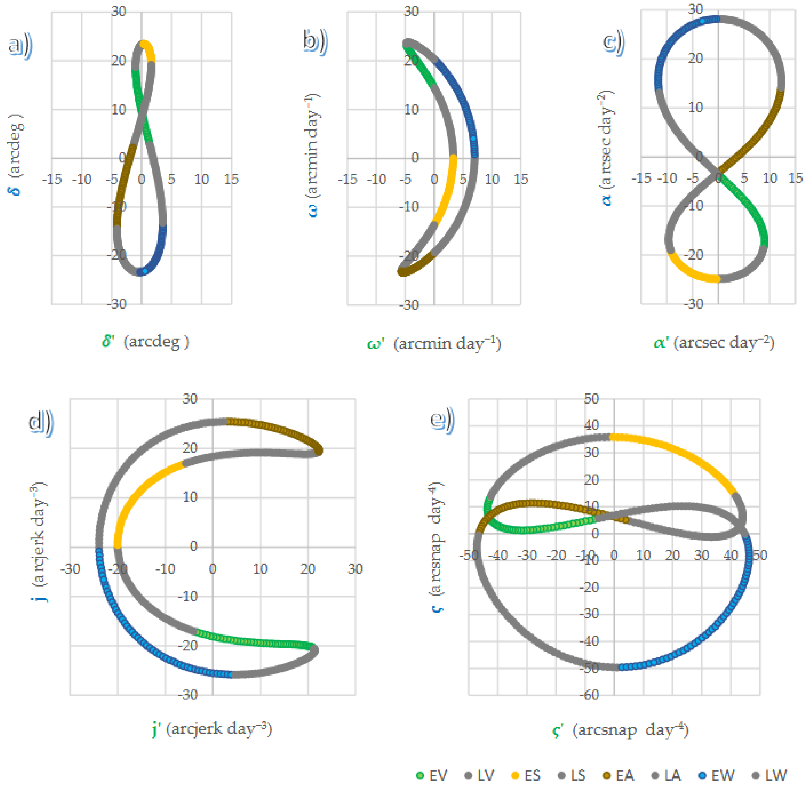
Figure 2.
Association between Earth’s circumference at the latitude holding NBI and Earth’s linear rotational speed (ERS) (a), then both given parameters plotted against day number within a Gregorian year (b), and finally, the association between the acceleration of the same parameters (c). V: Vernal S: Summer, A: Autumn, W: Winter, ERS: Earth’s rotational speed, NBI Natural Beam Irradiance.
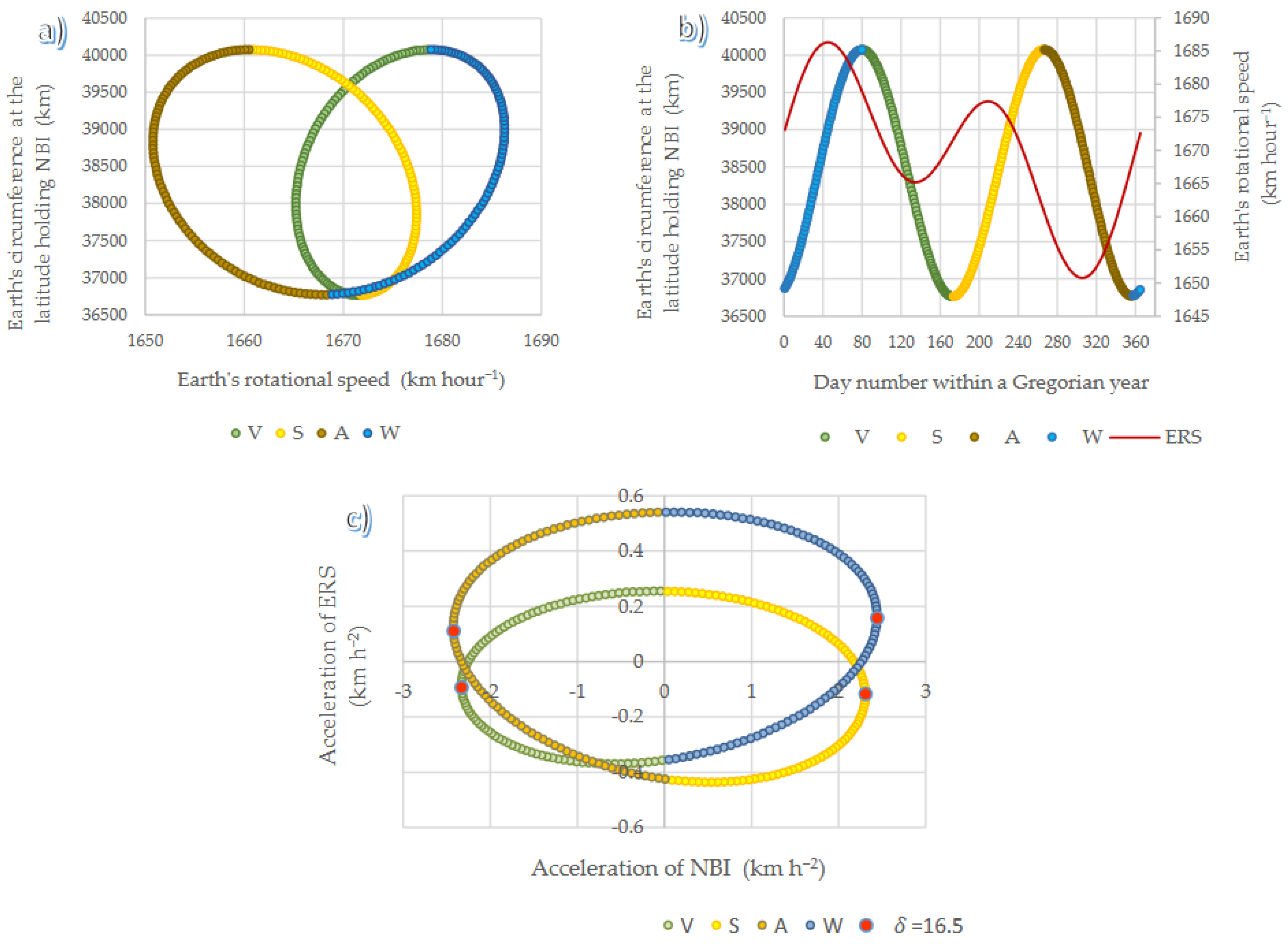

Table 1.
Parameters of the Sun’s vertical path for every season of the year: solar declination (), velocity (), acceleration (), jerk (), snap() and net drive ().
Table 1.
Parameters of the Sun’s vertical path for every season of the year: solar declination (), velocity (), acceleration (), jerk (), snap() and net drive ().
| Length (days) |
(arcdeg) |
(arcmin day−1) |
(arcsec day−2) |
(arcjerk day−3) |
(arcsnap day−4) |
||
|---|---|---|---|---|---|---|---|
| Spring | 93 | +14.969 | +15.048 | −15.416 | −15.355 | 14.206 | − |
| Summer | 93 | +14.815 | −15.097 | −14.934 | 15.416 | 12.377 | + |
| Autumn | 90 | −14.946 | −15.391 | +15.956 | 19.198 | −13.662 | − |
| Winter | 89 | −14.545 | +16.059 | +15.766 | −19.925 | −14.209 | + |
| Weighted average | 0.356 | −0.005 | 0.002 | −0.003 | −0.017 |
A negative net drive is decelerative, while a positive net drive is accelerative. The sign of the net drive is the sign of the product
Table 2.
Parameters of the Sun’s horizontal path by analemmatic section: equation of time (), velocity (), acceleration (), jerk (), snap(), net drive (), and Earth’s rotational speed ().
Table 2.
Parameters of the Sun’s horizontal path by analemmatic section: equation of time (), velocity (), acceleration (), jerk (), snap(), net drive (), and Earth’s rotational speed ().
| Period | Length (days) |
arcdeg |
(arcmin day−1) |
(arcsec day−2) |
(arcjerk day−3) |
(arcsnap day−4) |
km h−1 |
|
|---|---|---|---|---|---|---|---|---|
| Early spring | 47 | −0.129 | −3.007 | +6.083 | 11.284 | −31.860 | − | 1669.2 |
| Late spring | 38 | −0.488 | +2.118 | +5.227 | −14.057 | −25.659 | + | 1667.5 |
| Early summer | 36 | +1.172 | +2.146 | −5.366 | −15.134 | 23.282 | − | 1675.2 |
| Late summer | 52 | +0.569 | −3.512 | −6.596 | 10.972 | 32.590 | + | 1672.4 |
| Early autumn | 45 | −3.108 | −3.598 | +7.533 | 15.849 | −26.036 | − | 1655.5 |
| Late autumn | 52 | −2.700 | +4.435 | +8.064 | −14.248 | −30.721 | + | 1657.3 |
| Early winter | 52 | +2.186 | +4.403 | −7.957 | −13.075 | 32.492 | − | 1679.9 |
| Late winter | 43 | +2.773 | −3.057 | −6.810 | 15.946 | 23.700 | + | 1682.6 |
| Weighted average | 365 | −0.157 | 0.000 | 0.000 | 0.000 | 0.000 | 1669.8 |
The last column can be derived from in accordance with Equations (14), (15), and (17).
Table 3.
Signs of the main parameters and resultant drive of the Sun’s horizontal and vertical paths, according to a solar sundial noon analemma: position, velocity, acceleration and net drive.
Table 3.
Signs of the main parameters and resultant drive of the Sun’s horizontal and vertical paths, according to a solar sundial noon analemma: position, velocity, acceleration and net drive.
| Section | Sun’s horizontal path | Sun’s vertical path | Combined drive | ||||||
|---|---|---|---|---|---|---|---|---|---|
| Early spring | − | − | + | − | + | + | − | − | Coordinated |
| Late spring | − | + | + | + | + | + | − | − | Opposed |
| Early summer | + | + | − | − | + | − | − | + | Opposed |
| Late summer | + | − | − | + | + | − | − | + | Coordinated |
| Early autumn | − | − | + | − | − | − | + | − | Coordinated |
| Late autumn | − | + | + | + | − | − | + | − | Opposed |
| Early winter | + | + | − | − | − | + | + | + | Opposed |
| Late winter | + | − | − | + | − | + | + | + | Coordinated |
A negative net drive is named decelerative and a positive net drive is named accelerative. The net drives of the EoT and SMD are coordinated when they align (trans-equinoctial phases) or opposed when they differ (trans-solstitial phases).
Disclaimer/Publisher’s Note: The statements, opinions and data contained in all publications are solely those of the individual author(s) and contributor(s) and not of MDPI and/or the editor(s). MDPI and/or the editor(s) disclaim responsibility for any injury to people or property resulting from any ideas, methods, instructions or products referred to in the content. |
© 2025 by the authors. Licensee MDPI, Basel, Switzerland. This article is an open access article distributed under the terms and conditions of the Creative Commons Attribution (CC BY) license (http://creativecommons.org/licenses/by/4.0/).
Copyright: This open access article is published under a Creative Commons CC BY 4.0 license, which permit the free download, distribution, and reuse, provided that the author and preprint are cited in any reuse.


