
Submitted:
27 December 2024
Posted:
27 December 2024
You are already at the latest version
Abstract
The problem of using accounting semi-identity-based (ASI) models in Econometrics can be severe in certain circumstances, and estimations from OLS regressions in such models may not accu-rately reflect causal relationships. This dataset was generated through Monte Carlo simulations, which allowed for precise control of a causal relationship. The selected model for testing the in-fluence of the ASI problem is the Fazzari, Hubbard, and Petersen (1988) model, which seeks to establish a relationship between a company’s investments and its cash flows, and which is an ASI as well. The dataset included randomly-generated independent variables (cash flows and Tobin’s Q) to analyse how they influence the dependent variable (cash flows). The Monte Carlo meth-odology in Stata enabled repeated sampling to assess how ASIs affect regression models, high-lighting their impact on variable relationships and the unreliability of estimated coefficients. The purpose of this paper is twofold: its first goal is to provide a deeper explanation of the syntax in the related article, offering more insights into the ASI problem. The openly available dataset supports replication and further research on ASIs' effects in economic models and can be adapted for other ASI-based analyses, as the information comprised in the reusability examples prove. Second, our aim is to encourage research supported by Monte Carlo simulations, as they enable the modeling of a comprehensive ecosystem of economic relationships between variables. This allows researchers to address a variety of issues, such as partial correlations, heteroskedasticity, multicollinearity, autocorrelation, endogeneity, and more, while testing their impact on the true value of coefficients.
Keywords:
Monte Carlo simulation
; accounting semi-identities
; investment-cash flow sensitivity
; controlled causal relation
1. Summary
In financial management literature, it is widely accepted that a company’s annual cash flow significantly influences its investment decisions. The model proposed by Fazzari, Hubbard and Petersen (FHP hereinafter) (1988) explores this relationship using a linear regression framework, where the investment-cash flow sensitivity coefficient indicates the extent to which firms depend on internal funds for investments. Higher coefficients suggest greater financial constraints due to severe information asymmetry, making external financing costly or inaccessible.
The data of this work is related to the research article “A Cautionary Note on the Use of Accounting Semi-Identity-Based Models” Sánchez-Vidal (2023) [1], published in the Journal of Risk and Financial Management. In this related work Sánchez-Vidal (2023) critiques the FHP (1988) [2] model by identifying that the equation used is an Accounting Semi-Identity (ASI), a partial representation of an accounting identity that omits certain variables. This omission can introduce biases in econometric models, leading to inaccurate estimation of causal relationships. Specifically, excluding other components from the complete accounting identity may distort the estimated coefficient of cash flow, causing more financially constrained firms to appear less constrained in the results of the estimation
By generating synthetic data, Monte Carlo simulations allow to assess the impact of omitted variables in ASI-based models, by comparison between estimated and true coefficients, highlighting the limitations of the FHP model and providing a valuable tool for evaluating ASI-based models. The synthetic nature of this database is critical, because the alternative approach would involve using 'real' databases, allowing researchers to subsample the total sample into a priori more financially constrained firms and other companies based on any academically accepted criterion. Suppose the linear regression is run and produces higher coefficients for the financially constrained subset. However, researchers would still face the uncertainty of whether these results are due to the actual impact of financial constraints—which should lead highly constrained firms to depend more on internally generated funds—or whether the larger coefficients are solely a consequence of the limitations imposed by the ASI. This issue is addressed by using synthetic data, which gives the researcher full control to distinguish between results driven by causality and those influenced by the ASI problem. The accompanying dataset facilitates replication of the FHP (1988) model with similar or alternative parameters.
2. Methods and Data Description
As previously mentioned, the novelty of this work lies in the decision to use a randomly generated database instead of a real one, allowing for pinpoint control over the causal relationships. The approach used to create the data combines a fixed (deterministic) economic model with random (Monte Carlo) simulations to handle uncertainty in input factors, all done using Stata software. Essentially, the explanatory variables that affect investments are generated using Monte Carlo simulations, and the investment values (dependent variable) are calculated by applying these randomly generated inputs to a model that explains how investments are determined.
2.1. Model for Generating Investments as a Function of Cash Flows and Tobin’s Q
The approach employed to produce the foundational data in this article combines a deterministic economic process model with Monte Carlo-based stochastic simulations to account for uncertainty in input parameters. This is done by utilizing assumption distributions grounded in literature and practical knowledge, all executed in Stata.
The simulation was designed by generating 50,000 sets of error terms using a normal distribution, each with a mean of zero and a standard deviation of 0.1. Additionally, 50,000 sets of a cash flow variable (CFi) were created, also normally distributed, with a mean of 0.25 and a standard deviation of 0.1. Another 50,000 sets of Tobin’s Q were generated, with a mean of 2.45 and a standard deviation of 0.2, along with a final 50,000 sets of error terms with a mean of zero and a standard deviation of 0.1. As is typical in Monte Carlo simulations, the selection of parameters is somewhat arbitrary [3]. Investments are calculated using the randomly generated values for cash flows, Tobin`s Q and the error term relating them to the investments in this way:
where i denotes value for the i-th company.
Invi = 0 + 0.45CFi + 0.03Qi +ɛi,
Since the goal is to test the model using Ordinary Least Squares (OLS), the choice of a normal distribution is appropriate. The true parameters in the synthetic relation of investments with cash flows and Tobin’s Q are chosen in a way the parameters of the variable -investments- are analogous to those in the seminal work of FHP (1988) from which the model we want to test comes from. The descriptive statistics of the randomly-generated cash flows, as well as the investments variable show means and standard deviations very similar to the values from the four subsamples of firms studied by Fazzari et al. (1988, pp. 22, 25) , as can be seen in Table 1. The concrete values used in this controlled relationship imply that, ceteris paribus, an increase in cash flows of the 20% would cause an increase in investments of the 9%.
All factors that could influence investments, and which are not considered in the FHP (1988) model are proxied by the error term ɛi [4]. These factors include broader macroeconomic conditions like interest rates and inflation, competitive forces within industries, regulatory changes, etc., all of which can shape investment behavior. The model also does not account for technological advancements, quality of management and corporate governance, or the availability of external financing [5], which are all crucial in determining a firm's investment strategy. Additionally, factors such as investor sentiment, supply chain disruptions, strategic considerations, and labor market conditions are not incorporated but can have a significant impact on investment decisions. One example is agency costs, where managers may be motivated to either overinvest or underinvest based on various corporate governance factors, as suggested by the free cash flow theory [6].
The inherent arbitrariness involved in constructing the investment-cash flow relationship [7] is typical of any simulated model. This approach is comparable to the Electric Scooter Project example found in a widely renowned finance handbook [7] (2003, p. 263). However, it offers the added benefit of high comparability with the original dataset from FHP’s seminal work (1988), due to the carefully chosen parameters for the randomly generated cash flows and the true coefficients of the synthetic relationship. Starting from this point, researchers can alter the distributions of the randomly generated variables and the features of the primary relationship to ensure they align with any newer research pertaining to this model.
Figure 1 displays a scatterplot of the cash flow and investment values for each observation, clearly illustrating the positive correlation between the two variables. Observing this graphical correlation is very illustrative, as its existence is negated by the ASI problem in certain estimations of OLS regressions, as demonstrated in the related article (Sánchez-Vidal, 2023).
2.2. Examples of Reusability
2.2.1. First Example: Controlling for Q
In the following paragraphs, I will provide an example of how this dataset can be reused. The aim is to utilize a subset of companies with similar Q ratios, thereby controlling for one of the factors that could influence investment decisions [2]. This approach enables a focused examination of the relationship between cash flows and investments, which represents the primary objective of this database and the associated research. This focus is particularly significant because both variables are integral to the ASI component in the FHP (1988) model, and the analysis of their relationship is framed within the context of the ASI problem.
As shown in the Stata syntax file associated with this article, I have selected companies in the highest quintile of Q values. Figure 2 illustrates the combinations of cash flows and investments for this subset of firms. In real-world scenarios, these high-Q firms—those valued in financial markets at significantly higher prices than their accounting values—are typically companies with highly valuable investment opportunities (Tobin, 1969) [8]. In Figure 2, I have highlighted two subsamples of companies, shown in brown and green, which will be analyzed further to confirm the ASI problem and the associated risks of using the ASI. The brown subset represents high-Q firms with cash flows below the overall sample mean (though still positive) and investments below the threshold of 0.1 (10%). In contrast, the green subset consists of companies with a similar combination of high Q and low cash flow generation but with investments exceeding 0.1.
For example, a company in the brown group might generate 0.08 in cash flows (considered low) and invest 0.08 (below the average), allocating all its available funds toward growth. This indicates a high reliance on internal cash flows to finance its investments. In contrast, a company in the green group might also generate 0.08 in cash flows but invest 0.16. This suggests it invests more due to better access to external funding sources, such as bank financing, which supplement its cash flow and enable higher levels of investment. The green subset, consisting of companies capable of making substantial investments despite limited cash flows, is clearly less financially constrained than the brown subset.
After defining these two groups in Stata, I perform a regression of investments on cash flows for each group. The results are displayed in Table 2.
The results in the first two columns reveal that companies with higher investments exhibit greater cash-flow sensitivity, a finding that contradicts both logical expectations and the predictions of the FHP (1988) model. As discussed in the related article, this inconsistency stems from issues introduced by the ASI problem. To analyze the two subsamples within a single regression framework, I constructed a multiplicative variable combining cash flows with a low/high investment dummy (1,0 respectively) and performed a unified regression analysis. The results, presented in the third column, indicate a lower sensitivity of investment to cash flows for the brown subsample, containing the more financially constrained companies (as shown by the sum of the coefficients for cash flows and the multiplicative variable). This reproducibility example underscores, once again, the ineffectiveness of using ASI-based models. Details on the creation of subsamples, the multiplicative variable, and the regression analysis for this exercise are provided in the accompanying syntax file.
2.2.2. Second Example: Decoupling Investments from Cash Flows
In the following paragraphs, I will recreate the same example, but this time I allow the investments variable to remain independent of cash flows while still being influenced by Q (Inv2i = 0 + 0.075Qi + ɛi). When running the regression, the coefficient aligns with expectations, as it is not significantly different from 0.075 at the 99% confidence level. However, this coefficient loses significance when the regression is applied only to a subsample of positive residuals (second column of Table 3), highlighting one of the issues associated with using ASIs: variables outside the ASI framework lose their significance in the presence of a dominant ASI
2.2.3. Third Example: Developing Other Model
The previously mentioned Scooter example [5] could be interesting to expand upon. This example involves analyzing a business plan in which Cash Flows: inflows and outflows, derived from revenues and costs, must be estimated. The handbook provides guidance on the characteristics of cash flow estimations, with a more detailed explanation for the Sales variable. For the sake of brevity, I will focus solely on the simulation of the sales variable. To fully simulate the complete cash flows variable, the researcher should recreate all components, incorporating all interrelationships between them. Sales are determined by the following formula:
REVENUES = MarketSize x MarketShare x UnitPrice
In this specific example, the market size is estimated at 1 million scooters for the first year, although the actual price is subject to estimation errors:
and where errorMS1 refers to the error in Market Size forecast in year 1
Market Size1 = ExpectedMarketSize1 x (1+errorMS1),
Here, errorMS1 refers to the error in the Market Size forecast. As expected, the Market Size for year t is calculated as the previous year's Market Size (t-1) multiplied by the forecasting error in year t. Due to the construction of this component, errors accumulate over time. In the example, the expected sales value is set at 100,000, but the actual amount could be 110,000, reflecting a forecast error of 10%. As “what happens in year 2 is affected by what happens in year 1,” a scenario where “scooter sales are below expectations in year 1, it is likely that they will continue to be below in subsequent years”.
Since the Sale estimations are made in year 0, forecasting further into the future becomes increasingly complex as errors compound. For instance, by year 4, the Market Size is forecasted using the following formula:
Market Size4 = ExpectedMarketSize1 x (1+errorMS1) x (1+errorMS2) x (1+errorMS3) x (1+errorMS4)
Monte Carlo simulations can be used to model this accumulation in panel data, as illustrated in the syntax, where a sales value is generated for each year. The example incorporates not only interdependence between periods but also interdependence between different variables. The authors suggest a correlation between Market Size and Price, noting that “the price of electrically powered scooters is likely to increase with market size.” For example, “a 10 percent shortfall in market size would lead to a predicted 3 percent reduction in price.” Using this relationship, the Price for the first year can be modeled as follows:
Price1 = Expected price1*(1+0.3*errorMS1)
In this way, errors accumulate over the years in a manner similar to sales.
Table 4 demonstrates the correlation between the two components of total revenues and Figure 3 shows the histogram of the simulated values for the cash flows variables of year 1 and year 10 respectively. Due to the method used to generate the yearly values, the standard deviations for different years are significantly different (this result not reported).
The researcher could then generate the remaining variables with various interrelated relationships and derive a probability distribution for the associated NPV after estimating all components of cash flows and the appropriate cost of capital.
As demonstrated, Monte Carlo simulations enable the development of more complex models, such as this Scooter example. In this model, the behavior of one of the components of cash flows (revenues) introduces autocorrelation, as a portion of sales depends on its previous values. Additionally, a potential heteroskedasticity issue may arise due to the accumulation of errors over time.
3. User Notes
This data descriptor relates to the use of Monte Carlo simulations to examine the relationship between cash flows and investments. Although Monte Carlo simulations are commonly used to test the validity of statistical tests [9], they can also be employed to generate a whole system of variables with crossed interrelations. The generated data of this work is designed to evaluate whether the regressions effectively capture the causal relationship, taking into account the constraints imposed by the accounting semi-identity (ASI). The Monte Carlo simulation process can be replicated to produce data that closely resembles or significantly diverges from that of Sánchez-Vidal (2023), as the examples 1 and 2 of reusability included in this works provides. This approach also allows for the generation of entirely new datasets to analyze alternative models, as demonstrated in the last reusability example.
The usefulness of these simulations for researchers in finance, as well as in other areas related to business and economics, is clear. The researcher always knows the true coefficient that measures the relationship between a variable and the independent variable that may affect it, allowing them to assess the importance of various issues that may arise in estimating this true coefficient. Additionally, the simulations enable the generation of panel data with autocorrelation (as shown in Example 3 of reusability), as well as other potential problems (multicollinearity, heteroskedasticity, etc.), and help calibrate the effectiveness of various potential solutions.
Supplementary Materials
The following supporting information can be downloaded at: www.mdpi.com/xxx/s1, Figure S1: title; Table S1: title; Video S1: title.
Funding
This research received no external funding
Data Availability Statement
Submitted within supplementary files.
Conflicts of Interest
The authors declare no conflicts of interest.
References
- Sánchez-Vidal, F.J. A cautionary note on the use of accounting semi-identity-based models. J. Risk Financ. Manag. 2023, 16, 389. [Google Scholar] [CrossRef]
- Fazzari, S.; Hubbard, R.G.; Petersen, B. Financing constraints and corporate investment. Cambridge: National Bureau of Economic Research 1988. [CrossRef]
- Carbone, E. Discriminating between Preference Functionals: A Monte Carlo Study. J. Risk Uncertain. 1997, 15, 29–54. [Google Scholar] [CrossRef]
- Gujarati, D.N.; Porter, D.C. (2013). Basic Econometrics. McGraw-Hill Irwin.
- Brealey, R.A. , Myers, S.C.; Allen, F. (2003). Principles of corporate finance. McGraw-hill.
- Rajan, R.G.; Zingales, L. Financial dependence and growth. Am. Econ. Rev. 1998, 88, 559–586. [Google Scholar] [CrossRef]
- Jensen, M. Agency costs of free cash flow, corporate finance, and takeovers. Am. Econ. Rev. 1986, 76, 323–329. [Google Scholar] [CrossRef]
- Tobin, J. A general equilibrium approach to monetary theory. J. Money Credit. Bank. 1969, 1, 15–29. [Google Scholar] [CrossRef]
- Dufour, J.M.; Khalaf, L. (2001). Monte Carlo test methods in econometrics. Companion to Theoretical Econometrics’, Blackwell Companions to Contemporary Economics, Basil Blackwell, Oxford, UK, 494-519.
Figure 1.
Scatterplot of cash flows (X) and investments (Y).
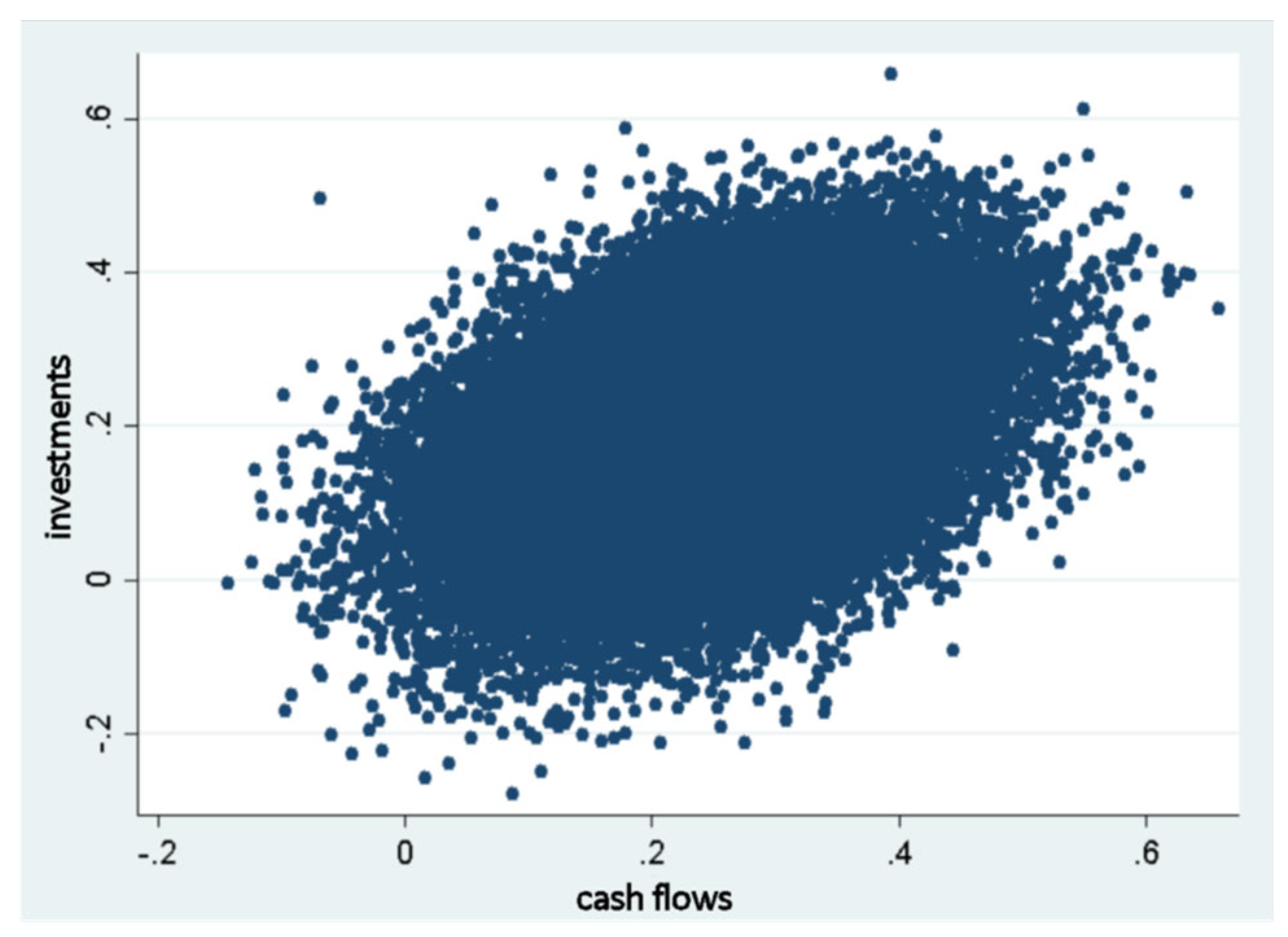
Figure 2.
Scatterplot of cash flows (X) and Investments (Y) for a subset of high Q companies.
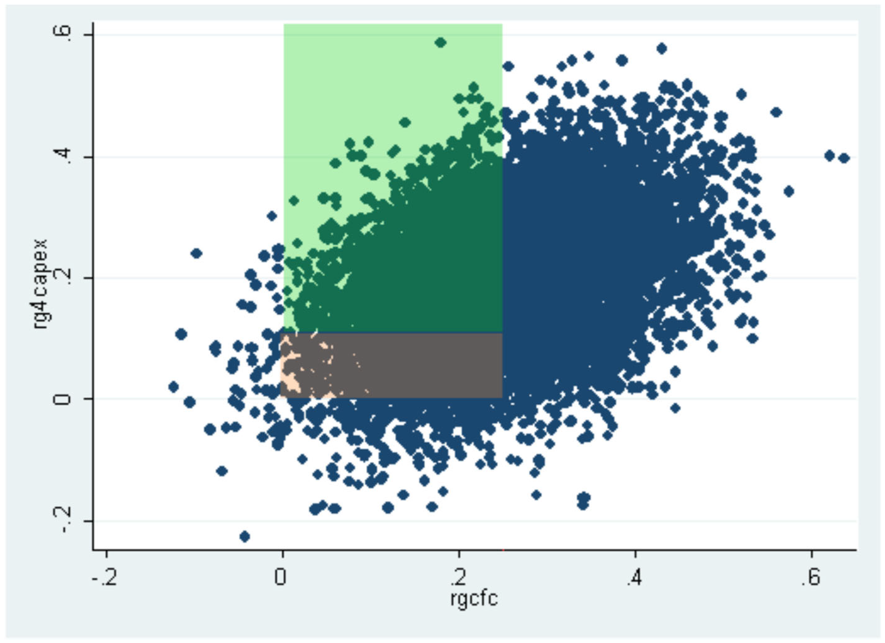
Figure 3.
Histogram of the simulated cash flows variable (in millions of yen) for years 1 (a) and 10 (b), respectively.
Figure 3.
Histogram of the simulated cash flows variable (in millions of yen) for years 1 (a) and 10 (b), respectively.
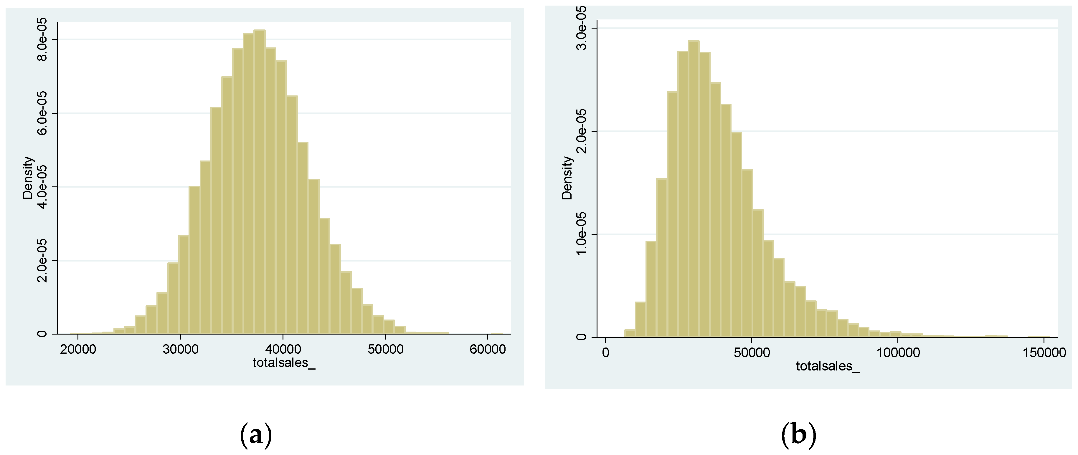

Table 1.
Descriptive statistics for the simulated variables.
| Variables’ names in the article | Variables’ names in the sintax | Mean | Median | SD | Min | 1st quartile |
3rd quartile | Max |
|---|---|---|---|---|---|---|---|---|
| Cash flows | rgcfc | 0.250 | 0.250 | 0.100 | -0.143 | 0.182 | 0.317 | 0.659 |
| Q | rgq | 2.450 | 2.450 | 0.200 | 1.634 | 2.316 | 2.585 | 3.276 |
| Investments | rgcapex | 0.187 | 0.187 | 0.110 | -0.280 | 0.113 | 0.261 | 0.658 |
| rest | rgres | -0.063 | -0.063 | 0.114 | -0.536 | -0.140 | 0.014 | 0.564 |
N observations: 50,000.
Table 2.
Results of OLS estimation for Equation 1 for a subset of high-Q, low-cash-flow companies. subsampled in low vs high investments.
Table 2.
Results of OLS estimation for Equation 1 for a subset of high-Q, low-cash-flow companies. subsampled in low vs high investments.
| Subsample low Investments (brown) |
Subsample high Investments (green) |
Whole sample |
||||
|---|---|---|---|---|---|---|
| Coef. | t | Coef. | t | Coef. | t | |
| Cash flow | 0.105*** | 4.47 | 0.232*** | 10.17 | 0.510*** | 28.27 |
| Dummy low invest x Cash flow | -0.910*** | -68.31 | ||||
| Constant | 0.021*** | 5.30 | 0.165*** | 38.55 | 0.111*** | 33.53 |
| R2 | 0.014 | 0.028 | 0.511 | |||
| N | 1306 | 3586 | 4892 | |||
Robust standard errors in parentheses. *** p < 0.01.
Table 3.
Results of OLS estimation for for a subset of investments independent of the cash flows variable.
Table 3.
Results of OLS estimation for for a subset of investments independent of the cash flows variable.
| Whole sample | Subsample for positive rest | |||
|---|---|---|---|---|
| Coef. | t | Coef. | t | |
| Cash flow | 0.002 | 0.38 | 0.558*** | 85.69 |
| Q | 0.076*** | 34.21 | 0.032 | 12.36 |
| Constant | -0.003 | -0.47 | 0.089*** | 13.74 |
| R2 | 0.023 | 0.323 | ||
| N | 50000 | 16109 | ||
Robust standard errors in parentheses. *** p < 0.01.
Table 4.
Correlation of sales and price.
| Sales (units) | Price | |
|---|---|---|
| Sales (units) | 1.000 | |
| Price | 0.992*** | 1.000 |
***: denotes significance at the 1 percent level.
Disclaimer/Publisher’s Note: The statements, opinions and data contained in all publications are solely those of the individual author(s) and contributor(s) and not of MDPI and/or the editor(s). MDPI and/or the editor(s) disclaim responsibility for any injury to people or property resulting from any ideas, methods, instructions or products referred to in the content. |
© 2024 by the authors. Licensee MDPI, Basel, Switzerland. This article is an open access article distributed under the terms and conditions of the Creative Commons Attribution (CC BY) license (http://creativecommons.org/licenses/by/4.0/).
Copyright: This open access article is published under a Creative Commons CC BY 4.0 license, which permit the free download, distribution, and reuse, provided that the author and preprint are cited in any reuse.


