1. Introduction
Immunization is a core component of primary healthcare service delivery, reducing vaccine preventable morbidity and mortality (Shattock et al., 2024) and critical to achieving the Sustainable Development Goals (United Nations, 2015) and other global health policy goals such as the Immunization Agenda 2030 (World Health Organization, 2020) and Gavi Strategy 5.0 (Gavi The Vaccine Alliance, 2020). Yet, immunization and other health services remain inaccessible to vulnerable and marginalized populations, including those living in remote rural areas, conflict and humanitarian settings and the urban poor (Chopra et al., 2020, UNICEF and the Bill and Melinda Gates Foundation, 2021, Wigley et al., 2022). To design effective intervention strategies to reach these populations, accurate spatially detailed maps of vaccination coverage and other health and development indicators (HDIs) such as maternal literacy, poverty, school attendance, malaria prevalence, malnutrition and skilled birth attendance (Bosco et al., 2017, Mosser et al., 2019, Weiss et al., 2019, Kinyoki et al., 2020, Sbarra et al., 2021) can be useful. These maps enable decision makers to better understand the inequities that exist in service coverage and utilization and enhance the targeting of population subgroups or entire populations in a more effective manner – a field of research known as precision public health (Dowell et al., 2016). Moreover, by providing current, reliable, robust and actionable evidence base, high-resolution maps of vaccination coverage and other HDIs help bridge the data gap that exist in many low- and middle-income countries where health management information systems and other administrative data sources such as vital registration are often incomplete and unreliable (Scobie et al., 2020, Mwinnyaa et al., 2021).
Data for producing maps of vaccination coverage and other HDIs often come from nationally representative, geolocated household surveys such as the Demographic and Health Surveys, Multiple Indicator Cluster Surveys and national vaccination coverage surveys. Due to high operational costs, most surveys are designed to be representative at the provincial level (i.e., the first administrative level), meaning that classical approaches for analyzing survey data such as direct weighted estimators (Rao, 2005) can only produce estimates at this level. However, accurate estimates are most useful at lower administrative levels, e.g., the district or second administrative level at which vaccination programs and other interventions are planned and implemented. This, alongside developments in geostatistical modelling and improvements in computing power, has led to a proliferation of geostatistical and machine learning (ML) approaches to produce gridded estimates of HDIs from survey data. These methods rely heavily on the direct and proximate relationships that exist between (cluster level) data on HDIs and geospatial covariate data, as well as spatial and spatiotemporal dependence, to model and predict the spatial distributions of HDIs for single or multiple timepoints. The production of estimates of HDIs at the grid level, typically at 1 km or 5 km resolution, means that these are not tied to inconstant political or administrative boundaries and can be easily aggregated to operationally relevant areas of interest. Also, when integrated with other geospatial datasets, e.g., population maps (Tatem, 2017) and geolocated health facility data (Lim et al., 2008, Johns et al., 2022), precise estimates of at-risk or underserved populations can be produced. Research and survey programs such as WorldPop through its VaxPop project(Utazi et al., 2018b, Utazi et al., 2019, Utazi et al., 2021, Utazi et al., 2022), the Institute for Health Metrics and Evaluation (IHME)(Mosser et al., 2019, Sbarra et al., 2021) and the DHS program (Janocha et al., 2021) now routinely produce and distribute maps of HDIs.
Popular geostatistical, ML and hybrid approaches for producing high-resolution maps of vaccination coverage and other HDIs include geostatistical models (GEOS) (Bosco et al., 2017, Utazi et al., 2021, Utazi et al., 2022, Alegana et al., 2024), generalized additive models (GAMs) (Takahashi et al., 2017, Kawakatsu et al., 2024), stacked generalization (STG) (Mosser et al., 2019, Sbarra et al., 2021), boosted regression trees (BRT) (Kawakatsu et al., 2024), random forests (Browne et al., 2021), least absolute shrinkage and selection operator (LASSO) regression and deep learning/artificial neural networks (ANN) (Bosco et al., 2017). Model-based geostatistics (Diggle et al., 1998) explicitly accounts for spatial autocorrelation and the (non)linear effects of covariates and is often fitted in a Bayesian framework using the INLA-SPDE approach or MCMC techniques, although the former has gained more popularity in recent times due to its computational benefits. When non-linear effects (or smooth functions) of covariates are included in a geostatistical model, a semiparametric geostatistical model (SGEOS) (Wood, 2011, Wang et al., 2018) which eliminates the need for covariate data transformation is obtained. Also, the Bayesian implementation of geostatistical models provides a natural framework to account for the uncertainties associated with the predictions, as well as the input data. ML and hybrid approaches are especially suitable for modelling complex nonlinear relationships and interactions in the data, but this can sometimes result in a loss of interpretability. ML can automatically identify the relevant covariates/features in the data, unlike geostatistical modelling which may require a separate covariate selection process. Whilst ML approaches rely only on covariates to make predictions and would be expected to perform well if these are highly informative, geostatistical and hybrid approaches additionally leverage residual spatial (and temporal) autocorrelation. ML approaches are computationally less demanding, can handle large-scale and high-dimensional data better, and are sometimes less challenging to implement (e.g., GAM, LASSO and BRT) (James et al., 2013, Berrocal et al., 2020). However, some ML approaches such as BRT, ANN and LASSO do not produce uncertainty estimates, leaving users with the task of exploring additional techniques to quantify these uncertainties (Veronesi and Schillaci, 2019, Berrocal et al., 2020).
Currently, little is known about the comparative predictive performance of these ML and geostatistical approaches, especially in the context of mapping vaccination coverage. There is a lack of substantial evidence on how much the predicted maps produced by these approaches differ and which approaches yield more reliable estimates. This is likely due to the effort and technical expertise required to execute the different approaches and a cavalier attitude to methodological rigour. As maps of vaccination coverage and other HDIs become increasingly popular, it is imperative to better understand the advantages and limitations of each modelling approach. The goal of this study is, therefore, to critically evaluate these popular approaches for mapping vaccination coverage and other HDIs in terms of their predictive accuracy and associated uncertainties. We investigate four machine learning approaches (ANN, BRT, GAM and LASSO), two geostatistical models (GEOS and SGEOS) and one hybrid approach (STG). Our evaluation is based on a case study mapping the coverage of the first dose of the diphtheria-tetanus-pertussis (DTP1) and the first dose of the measles-containing vaccine (MCV1) vaccines using the 2018 Nigeria Demographic and Health Survey (NDHS) (National Population Commission - NPC and ICF, 2019).
2. Methodology
2.1. Data
2.1.1. Vaccination Coverage Data
Data on the coverage of DTP1 and MCV1 vaccines were obtained from the 2018 NDHS (National Population Commission - NPC and ICF, 2019) for children aged 12-23 months and 9-35 months, respectively. The NDHS was conducted between August and December 2018 and utilized a stratified, two-stage sampling design to produce estimates of indicators at the national, regional and state levels, and for urban and rural areas. Stratification was achieved by separating each of the 36 states and the Federal Capital Territory (FCT) into urban and rural areas. Samples were drawn from within each stratum in two stages: the first stage involved the selection of survey clusters (enumeration areas) from a national sampling frame using a probability proportional to size sampling scheme, while the second stage involved selecting households randomly from household lists within the selected clusters. Detailed information on the methods employed in the survey is published elsewhere (National Population Commission - NPC and ICF, 2019). The NDHS was selected because of ease of data access and having been used extensively in previous work to map coverage (Dong and Wakefield, 2021, Aheto et al., 2023, Utazi et al., 2023, Kawakatsu et al., 2024).
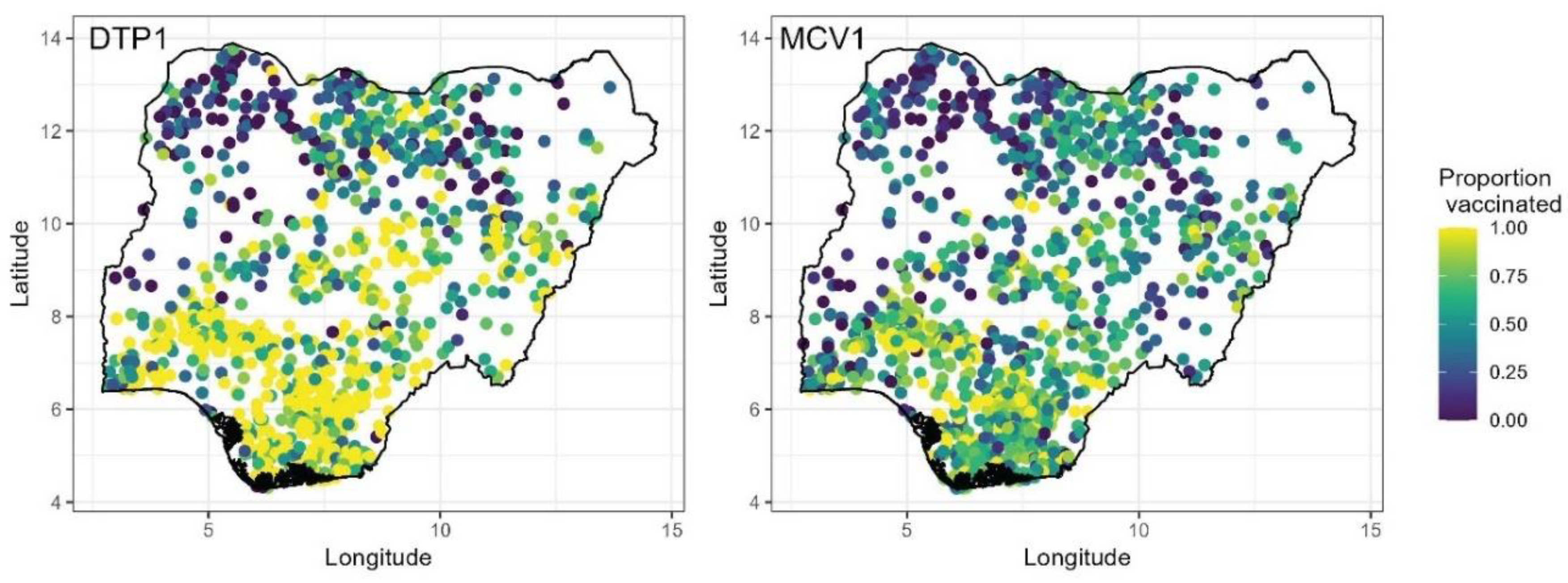
The survey was implemented in a total of 1389 clusters, with 11 of the 1400 clusters selected initially dropped due to security reasons. Also, in Borno State, only 11 of the 27 local government areas were considered in the survey due to high insecurity. For each vaccine, we used information obtained from both home-based records and maternal/caregiver recall, following DHS guidance during data extraction (Croft et al., 2023). Hence, our analysis captures crude DTP1 and MCV1 coverage estimates (World Health Organization, 2018). At the cluster level, we aggregated the individual level data to produce numbers of children surveyed, numbers vaccinated and empirical proportions of children vaccinated as shown in
Figure 1.
2.1.2. Geospatial Covariate and Population Data
To enhance the prediction of vaccination coverage using the approaches investigated, we obtained some geospatial covariate information — see supplementary Figures S1 and S2 and supplementary Table 1. These covariates have been successfully used in previous work (Bosco et al., 2017, Utazi et al., 2019, Utazi et al., 2022, Utazi et al., 2023) to model and predict vaccination coverage and other HDIs. These comprise variables measuring a range of conditions in the study country which may have direct or proximate relationships with vaccination coverage. These include remoteness (travel time to the nearest health facility and distance to cultivated areas), socioeconomic (poverty index, household wealth, maternal education), health (ownership of health or vaccination card/document, skilled birth attendance, access to media and use of mobile phone/internet) and urbanicity/development (nightlight intensity and urban/rural areas) variables.
The externally sourced geospatial covariates (supplementary Table 1) were processed and harmonized at 1 × 1 km resolution, at which we planned to produce grid level coverage estimates. To extract the values of the covariates for each cluster location, we used the approach described in Utazi et al (Utazi et al., 2018b) and Perez-Haydrich et al (Perez-Haydrich et al., 2013) which accounts for the displacement of the clusters (this displacement often occurs within districts in DHS surveys). For the DHS-derived covariates, we first calculated their values at the cluster level using detailed definitions provided in supplementary Table 1 and then used the krig() function in the fields package in R (Nychka et al., 2017) to create corresponding 1 × 1 km interpolated surfaces, with the optimal range parameter set to the first quartile of the distances between the clusters (other distance quartiles yielded almost the same results). The kriging interpolation was carried out using the logit-transformed cluster level data in each case due to its underlying Gaussian assumption, after which the estimates were back-transformed to the unit interval.
We checked for multicollinearity by examining the correlations between the covariates and by fitting non-spatial binomial regression models to estimate their variance inflation factors (VIFs). All the covariates included in the study had VIF values less than 5.0 for both vaccination coverage indicators, i.e., DTP1 and MCV1. Furthermore, for one of the modelling approaches (equations (1) and (2)), we examined the distributions of the covariates and their relationships with vaccination coverage (on the empirical logit scale), following which we log- or logit-transformed some skewed covariates to improve their linear relationships with vaccination coverage. The plots of the covariates and their relationships with vaccination coverage are shown in supplementary Figures S3 and S4. All 14 covariates were used in our study, as VIFs were acceptable and to facilitate using the ML approaches, as they are often trained using ample covariate information.
To aggregate the coverage estimates to the district and other administrative levels, we obtained 2018 gridded estimates of numbers of children aged under 5 years from WorldPop (Tatem, 2017), which we used as a proxy population layer for the age groups included in the study.
2.2. Geostatistical and Machine Learning Modelling Approaches
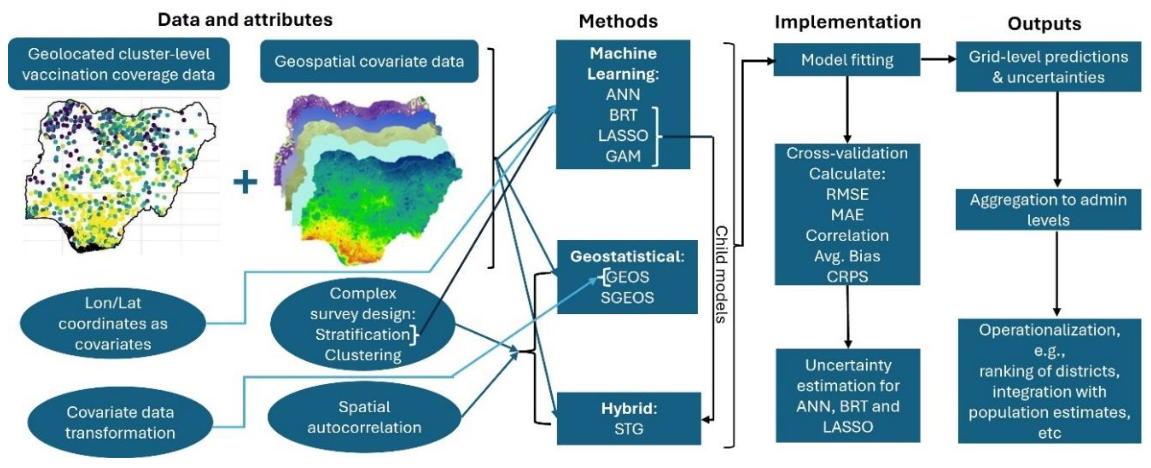
We consider seven modelling approaches to predict vaccination coverage at 1x1 km resolution as indicated previously. In all analyses, we accounted for the NDHS complex sampling design, namely urban-rural stratification by including an urban-rural covariate and, when using geostatistical modelling approaches, between-cluster variation (Dong and Wakefield, 2021, Gascoigne et al., 2025). The modelling approaches are described in detail as follows and illustrated in
Figure 2.
2.2.1. Bayesian Geostatistical Regression Model (GEOS)
The first model that we consider is a Bayesian geostatistical model with a Binomial likelihood. Letting
denote the number of children vaccinated at survey location
and
the number of children sampled at the location, the first level of the model assumes that
where
is the true vaccination coverage at location
We model
using the logistic regression model
where
is a vector of covariate data associated with
which includes an urban-rural covariate,
is a vector of the corresponding regression coefficients,
is an independent and identically distributed (iid) Gaussian random effect with variance,
, used to model non-spatial residual variation or between-cluster variation, and
is a Gaussian spatial random effect used to capture residual spatial correlation in the model. That is,
, where
is assumed to follow the Matérn covariance function (Matérn, 1960) given by
. The notation
denotes the Euclidean distance
is the marginal variance of the spatial process,
is a scaling parameter related to the range
– the distance at which spatial correlation is close to 0.1, and
is the modified Bessel function of the second kind and order
. For identifiability reasons, we set the smoothing parameter,
, see (Lindgren et al., 2011).
We complete the Bayesian model specification of the model by assigning a prior to the regression parameter, , and a penalized complexity (PC) (Simpson et al., 2017) prior to such that . Similarly, following Fuglstad et al (Fuglstad et al., 2019), we placed a joint PC prior on the covariance parameters of the spatial random effect, , such that and , with chosen to be the 5% of the extent of the country in the north-south direction.
The model was fitted using the INLA-SPDE approach implemented in the R-INLA package (Lindgren et al., 2015, R Core Team, 2021). The INLA approach – a faster alternative to MCMC – performs approximate Bayesian inference through a numerical approximation of the marginal posterior distributions of each unknow quantity in the model. The SPDE approach works by representing as a Gaussian Markov random field to reduce the computational burden associated with the estimation of (Lindgren et al., 2011). Predictions at 1x1 km resolution were obtained using the fitted model by drawing samples from the posterior predictive distributions of at the grid locations. Throughout, predictions at the administrative level were obtained as population-weighted averages taken over all the grid cells falling within each administrative area (Utazi et al., 2022).
2.2.2. Bayesian Semiparametric Geostatistical Regression Model (SGEOS)
This model extends the GEOS model in equations (1) and (2) through using smooth functions to account for the nonlinear effects of some covariates. The model assumes that the true vaccination coverage at location
,
, can be expressed as
where
is an intercept term,
are linear covariates with regression coefficients
, and
are smooth functions used to account for the non-linear effects of the covariates
. Other terms in the model are as defined previously in equation (2). We specify a second-order random walk prior for
such that
which is the Bayesian equivalent of a cubic smoothing spline (Wang et al., 2018) For identifiability, a sum-to-zero constraint is imposed on each of the smooth functions since the model includes an intercept term (Wang et al., 2018). Model (3) was also fitted in a Bayesian framework using the INLA-SPDE approach. During implementation, where necessary, we used the
inla.group()function to bin the covariates into groups according to both their cluster and grid level values, using the quantile option. We then extracted the computed values of the smooth function
for each grouped data point which were used to make predictions post model-fitting.
2.2.3. Generalized Additive Model (GAM)
Generalized additive models also provide a mechanism to account for non-linear relationships by allowing non-linear functions of all continuous covariates whilst maintaining additivity. The model is given by
where
denotes the urban-rural covariate and
are functions used to account for the non-linear effects of other covariates. For our analyses, we chose cubic smoothing splines for
, noting that other choices are also possible (James et al., 2013). The function
is used to account for the effect of space in the model, for which we specified a two-dimensional smoother - an isotropic smooth of latitude and longitude on the sphere with a second-order penalty (Wahba, 1981). The model was fitted in a frequentist framework and implemented in R using the mgcv package (Wood and Wood, 2015).
2.2.4. Boosted Regression Model/Trees (BRT)
Boosting is a tree-based method that also allows modelling complex, non-linear relationships between an outcome variable and various predictor variables (James et al., 2013). The method is based on the generation of a collection of sequentially fitted regression trees that optimize the predictive value of the response variable based on local predictor values. The boosting algorithm proceeds by fitting a regression tree to the data using the outcome variable as the response in the first iteration. The fitted tree is then scaled by a shrinkage parameter and added to the fitted function (this is set equal to zero in the first iteration) to update the residuals. In subsequent iterations of the algorithm, the regression trees are fitted using the residuals as the response. The process continues until a desired number of iterations or trees have been fitted. The output from the boosted model for location
can be expressed as
where,
denotes the final prediction from the model,
is the prediction from the
th component regression tree,
is a shrinkage parameter and
is the number of trees/iterations.
controls the rate at which the boosting learns and is usually chosen to be small. For our application, we set
as recommended in (James et al., 2013) and chose
. Another important tuning parameter when fitting a boosting model is the number of splits in each tree or the interaction depth, which controls the complexity of the boosted ensemble. This is often set equal to the default value of 1. The BRT model is implemented in our study using the gbm package in R (Ridgeway and Ridgeway, 2004). Due to the unavailability of the binomial distribution in the gbm package, we elected to model the logit-transformed cluster level vaccination coverage
using a Gaussian distribution and then back-transformed all the predictions post model-fitting. We note that as in model (5), the set of covariates used in fitting the model included the longitude and latitude coordinates to account for spatial variation.
2.2.5. Least Absolute Shrinkage and Selection Operator (LASSO) Regression
Lasso regression performs both variable selection and regularization and is particularly suitable for modelling contexts where a large or considerable number of covariates are available. The method implements automatic covariate selection through a penalty term (the
penalty) included in its objective function, which uses a tuning or regularization parameter to control the amount of regularization, i.e., how much the regression coefficients are shrunken towards zero. The method finds regression coefficients
that minimize the objective function
where
is the regularization parameter and all other terms are as defined previously. The first term in (7) is the log-likelihood function which can be obtained from the binomial regression model in equations (1) and (2) when the spatial and non-spatial random effects are excluded. Sufficiently large values of
will force some regression coefficients to be equal to zero. In practice,
is chosen via a grid search using cross-validation techniques. As in the GAM approach, the covariate data considered in the analysis using (7) included the longitude and latitude coordinates of the data locations. The LASSO regression model was implemented in our work using the glmnet package in R (Friedman et al., 2021).
2.2.6. Stacked Generalization Using a Bayesian Geostatistical Model (STG)
In statistical learning, stacked generalisation or stacked regression is an ensemble method for combining predictions from multiple models, often referred to as child models. In the hybrid variant implemented in our work, the child models are different ML approaches, predictions from which are combined using a geostatistical model (Bhatt et al., 2017, Mosser et al., 2019, Sbarra et al., 2021). Through these child models, the STG approach accounts for complex, nonlinear relationships between the covariates and the outcome. The geostatistical modelling framework is then used to account for residual spatial autocorrelation. The STG approach was proposed/utilized in (Bhatt et al., 2017) and has been used to model vaccination coverage and various HDIs (Mayala et al., 2019, Mosser et al., 2019, Sbarra et al., 2021).
Following Sbarra et al (Sbarra et al., 2021), we considered the following child models: GAM, BRT and LASSO regression. These child models were implemented as described previously, but excluding the geographical coordinates of the data locations in the covariate data. To obtain final predictions for the outcome, the predictions from these child models are included as covariates in the geostatistical model:
where
and
are regression coefficients and other terms are as described previously in equation (2). As in (Mosser et al., 2019, Sbarra et al., 2021), a sum-to-one constraint is imposed on the regression coefficients corresponding to the child models, such that
. This constraint helps to mitigate the effect of extreme predictions in the child models (Bhatt et al., 2017, Mosser et al., 2019, Sbarra et al., 2021) included in (8). As is usually the case in stacked generalization, Bhatt et al (Bhatt et al., 2017, Mosser et al., 2019, Sbarra et al., 2021) recommended the use of K-fold cross-validation predictions from the child models to calibrate the model (i.e., estimate the parameters) in (8), and then refitting the child models using the full data and using the predictions from these in (8) without refitting the model. We noted that using the cross-validation predictions from the child models in (8) compared to the full data predictions did not necessarily yield improvements in predictive performance in our analyses. The STG approach was implemented in our work using the INLA-SPDE approach and the INLABRU package in R (Lindgren et al., 2024).
2.2.7. Artificial Neural Networks (ANN)
An artificial neural network (ANN) is a ML technique that mimics the functioning of the animal brain. An ANN model is particularly useful in modelling contexts where data are large and complex, with potential nonlinearities and interactions between the covariates. The network consists of layers of connected neurons that serve as data processing units, where each neuron applies a linear transformation to its inputs, followed by a non-linear activation function. For our work, we used a multilayer perceptron network (Park and Lek, 2016), which consists of an input layer, multiple hidden layers and an output layer. The input layer receives the features from the data, processes and transmits these to the hidden layers which process the information further through interconnected neurons, while the output layer produces the final predictions. For a spatial location
with covariate vector
the predicted value from an ANN with a single hidden layer can be expressed as:
where
and
are the numbers of neurons in the input and hidden layers, respectively,
is the activation function,
and
are bias and weight parameters estimated to minimize mean squared error in the training data. Furthermore,
,
and
are outputs from the layers as shown in equation (9).
Fitting an ANN requires tuning the number of hidden layers, the number of neurons in each layer, and choosing the activation function. Other parameters such as the number of epochs (the number of times the entire data is passed through the network during training), stopping metric, stopping tolerance and stopping rounds are also tuned during model fitting. These early stopping criteria help to avoid overfitting in the model. A common choice for the activation function is the rectified linear unit (relu), defined as . The model was fitted using the h2o.deeplearning() function in the H2O package in R (Fryda et al., 2024). Since the H2O package does not support the binomial distribution, we elected to model the logit-transformed cluster-level vaccination coverage, denoted by in equation (9) using a Gaussian distribution and then back-transformed the predictions post model fitting. Based on a hold-out cross-validation exercise with an 80% training and 20% testing split, the final selected model has two hidden layers with, with 100 neurons each, with the number of epochs set to 100. The chosen stopping metric was the root mean square error (RMSE) while the stopping tolerance and rounds were set equal to 0.001 and 5, respectively. We checked the sensitivity of these choices by running several cases with different justifiable parameter values but obtained the same results each time.
2.3. Uncertainty Estimation Using Delete-a-Block Jackknife Cross-Validation
To estimate the uncertainties associated with the ML approaches: BRT, LASSO and ANN, we employed a delete-a-block jackknife technique. This is a variant of the delete-1 jackknife (Wang and Yu, 2021) in which a block of observations is deleted at a time. The spatial blocks were formed by drawing observations at random from the observed data. These can also be formed using spatially contiguous observations, but this approach is more likely to affect the underlying spatial structure in the data and can potentially introduce some artificial patterns in the uncertainty estimates, depending on the sizes of the blocks. The choice of the block size was guided by the need to have as many iterations as computationally logical (relative to the number of observations in the data) whilst preserving the underlying spatial correlation in the data. Having many iterations ensures stability in the results (i.e., the uncertainty estimates) and also reduces the numbers of observations deleted at each iteration. We noted during test runs that block sizes of up to observations produced variogram estimates that were very similar to those of the full data in our applications (supplementary Figures S5 and S6). We also noted that there were no material differences in the estimates obtained for numbers of replicates . We, therefore, set in our work, corresponding to block sizes of , where is the number of observations or spatial locations in the data as defined previously in (1). For all three ML approaches, we obtained the jackknife estimates of the uncertainties (i.e., the standard deviations) associated with the grid level predictions as , where is the th coverage estimate for grid location and is the jackknife estimate of the mean across all the replicates.
2.4. Model Validation Using k-Fold Cross-Validation and Variogram Analysis
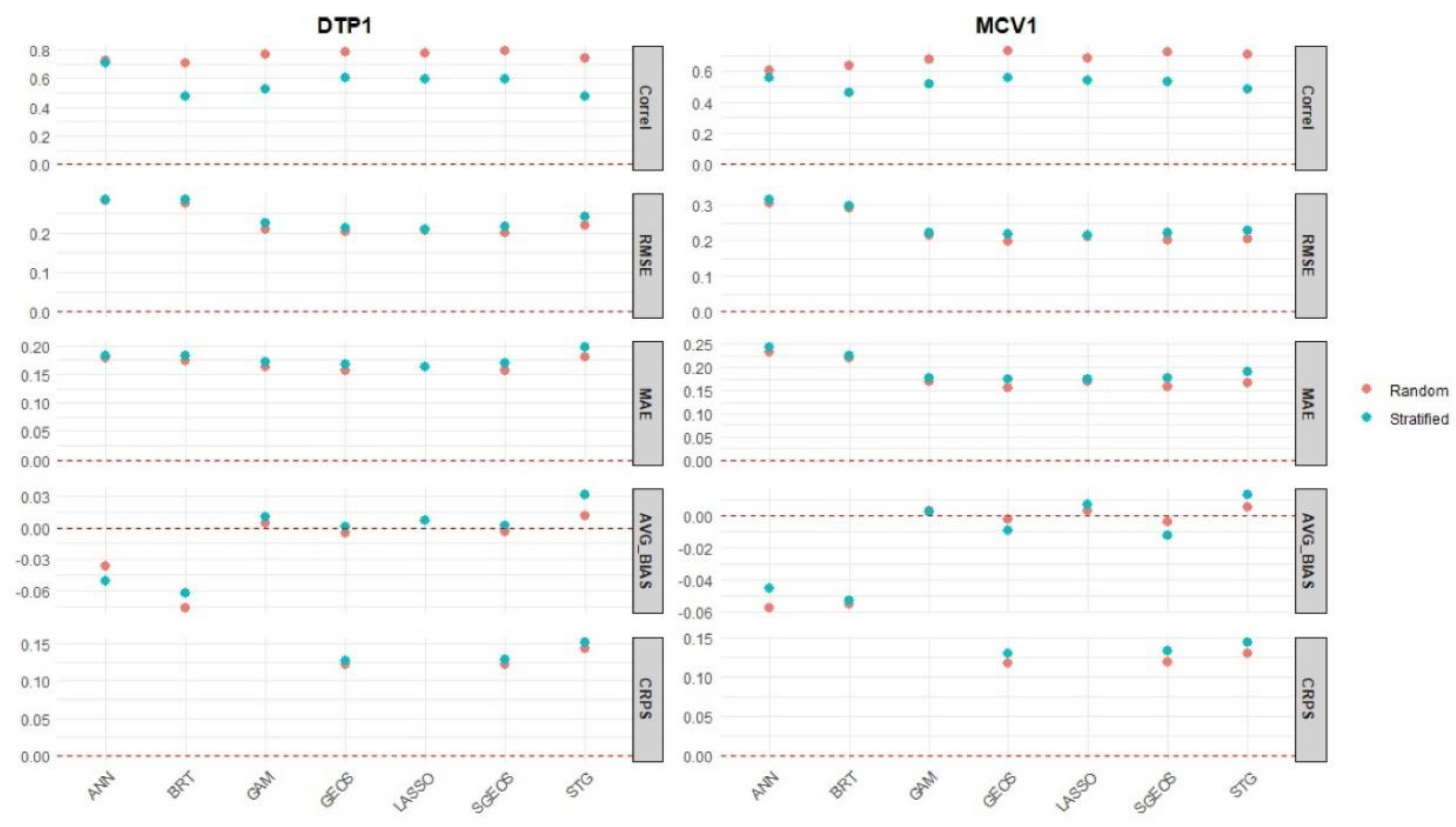
To evaluate the out-of-sample predictive performance of the modelling approaches, we conducted a -fold cross-validation exercise, setting . For each indicator-method combination, we created the cross-validation folds in two ways: random folds and spatially stratified folds. For the random folds, the survey locations were assigned to each of the folds in a random manner; whereas with the spatially stratified method, each fold comprised neighbouring cluster locations. We calculated the following measures of predictive performance: the correlation between observed and predicted values, root mean square error , mean absolute error , average bias and the continuous ranked probability score ( {REF}, where is the cumulative distribution function corresponding to the predictive distribution of the th cluster level estimate, and and are two independent random variables distributed according to . With posterior samples, the CRPS can be estimated as , which is then averaged over all the locations within each fold and over all the folds. While the other metrics (also averaged over all the folds) measure the accuracy of the point predictions produced by the approaches, the CRPS measures the accuracy of both the point and uncertainty estimates as it utilizes the entire posterior predictive distribution to determine the discrepancies between the observations and the predictions. Also, the CRPS is only computed for the three Bayesian approaches (GEOS, SGEOS and STG) in our work as it requires the posterior distributions of the estimates. The closer the AVG_, MAE and RMSE estimates are to zero and the smaller the CRPS, the better the predictions. Correlation values closer to one indicate better predictive ability.
Additionally, to further examine the fits of the different methods, we checked their (standardized) in-sample residuals for spatial autocorrelation using variograms and the associated variogram envelopes, which were obtained by permutation, using the geoR package in R (Ribeiro Jr et al., 2024).
3. Results
3.1. In- and Out-of-Sample Predictive Performance Using Cross-Validation and Variogram Analysis
With respect to the metrics used to evaluate the accuracy of the point estimates produced by the methods at the cluster level (correlation, RMSE, MAE and AVG_BIAS), we found that GEOS, SGEOS and, to a great extent, LASSO had the best out-of-sample predictive performance in most cases (
Figure 3 and Table 2). The values of these metrics for GAM and STG were also very close to those of the three best approaches, indicating only slightly worse predictive performance. BRT and ANN generally had the worst predictive performance, which can be clearly seen when considering the AVG_Bias and RMSE estimates in
Figure 3.
Among the three Bayesian approaches for which we computed the CRPS metric, we found that GEOS and SGEOS outperformed the STG method based on this metric, which is also consistent with the results obtained using the other metrics. All the methods had fairly similar predictive performance under the two types of cross-validation folds investigated (i.e., random and spatially stratified folds) according to all the metrics except the correlations which showed that nearly all the methods had better predictive performance under the random folds. These results indicate that the methods can reasonably predict not only random but also spatial blocks of missing values in unsampled areas. There was no evidence of improved predictive performance for MCV1 despite having relatively larger cluster level sample sizes than DTP1 ( Figure S7). This is likely due to the cluster level sample sizes for MCV1 not being large enough to induce noticeable improvements in predictive performance.
Furthermore, when examining the out-of-sample predictions in low coverage areas (i. e., areas with cluster level proportions - supplementary Figures S8 and S9), we found that the prediction errors (RMSE, random folds) for ANN and BRT were consistently larger () than those of the other approaches (0.24 RMSE 0.3), although there was evidence of overestimation in all the approaches. For DTP1, the lowest prediction errors were obtained for the GEOS and SGEOS methods, whereas for MCV1, these were obtained for SGEOS, GEOS and STG.
The variograms of the in-sample residuals for DTP1 and MCV1 shown in supplementary Figures S10 and S11 indicate that of all seven approaches investigated, there was strong evidence of residual spatial autocorrelation in the ANN and BRT methods. The variograms for both methods closely resembled those of the outcome variables (i. e., the cluster level proportions of vaccinated children – supplementary Figures S5 and S6). Also, the lack of evidence of spatial autocorrelation in the residuals is strongest for the geostatistical approaches – GEOS, SGEOS and STG.
3.2. 1x1 km Estimates of Vaccination Coverage and Associated Uncertainties
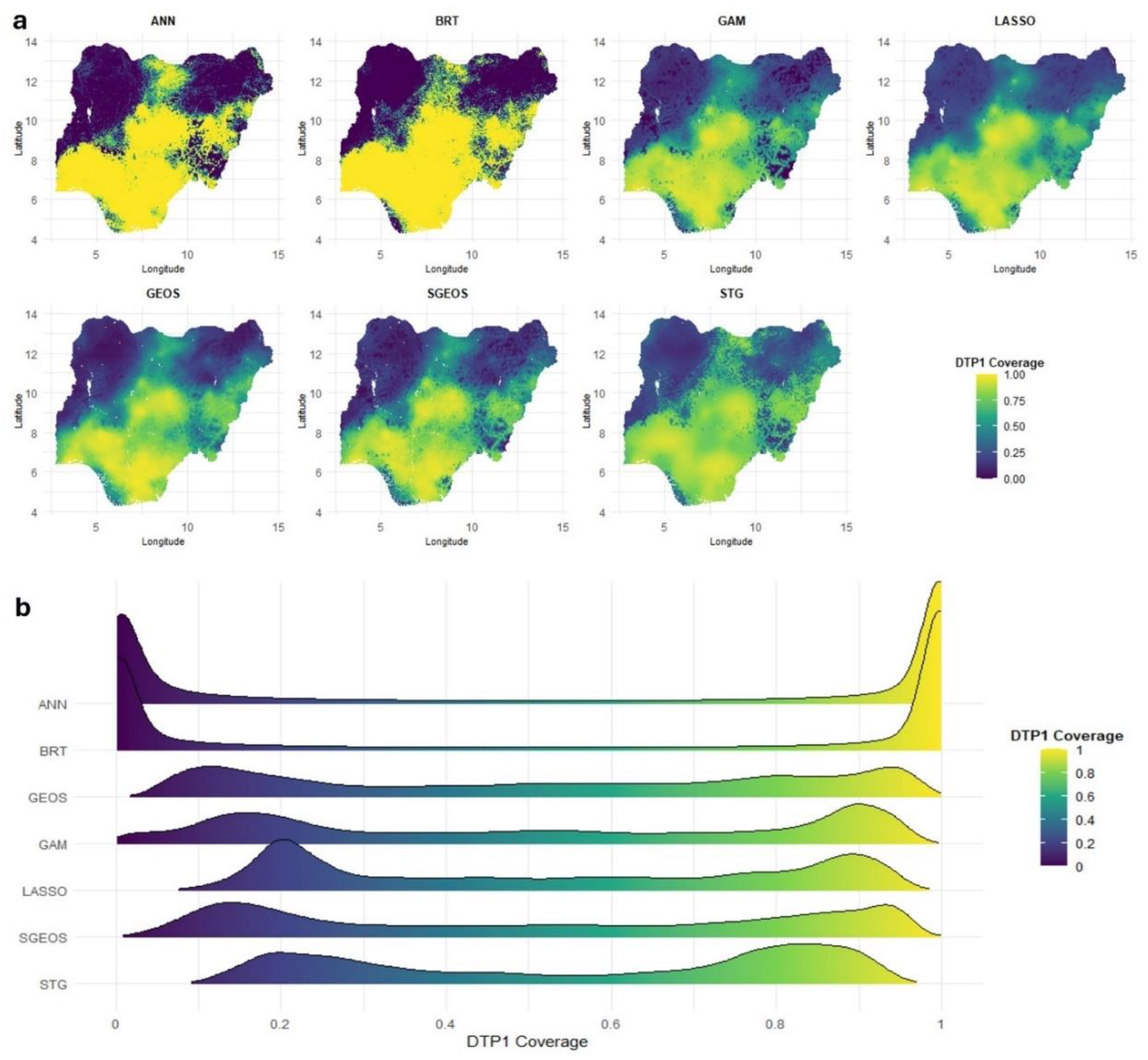
The rationale for the differences observed in the out-of-sample predictive performance of the approaches is apparent when investigating the 1x1 km predicted maps of vaccination coverage and associated uncertainties produced through using these approaches.
Figure 4 (a) shows strong similarities between the predicted surfaces produced by GAM, LASSO, GEOS, SGEOS and STG. Broadly similar patterns demonstrating a north-south divide in coverage can also be seen in the predicted maps produced using ANN and BRT, but their estimates are closer to the extremes of the unit interval and smoother in the lower and higher coverage areas than those of the other approaches.
The over-smoothing of the coverage estimates by ANN and BRT relative to the other approaches is evident in the distributions of the grid level DTP1 predictions shown in
Figure 4 (b). All the methods produced bimodal distributions reflecting the characteristic spatial distribution of vaccination coverage in Nigeria {REFs}. However, the grid level estimates produced by ANN and BRT are more peaked near zero and one than those produced by the other approaches, suggesting overestimation in high coverage areas and underestimation in low coverage areas by both approaches. This also explains the higher AVG_BIAS and RMSE values for both approaches relative to other approaches. For MCV1, supplementary Figures S12 (a-b) show similar patterns in the grid level estimates produced by all the approaches, with strong evidence of over-smoothing in low and high coverage areas by ANN and BRT relative to the other approaches.
The uncertainties associated with the predictions have broadly similar spatial patterns across the methods, with lower uncertainties in areas where coverage estimates are either close to the endpoints (an artefact of the binomial distribution) of the unit interval or where data locations are dense, and higher uncertainties in areas where the estimates are closer to 0.5 or where data locations are sparse (
Figure 5 (a) and (b)).
However, due to the over-smoothing by ANN and BRT, the uncertainties associated with both approaches are much smaller than those of other approaches (
Figure 5 (b)) in areas of lower and higher coverage, even in comparison with LASSO for which we used the same jackknife approach to produce its uncertainty estimates. In areas with mid-level coverage estimates, the uncertainties associated with the estimates produced by BRT are noisier and relatively much higher than other approaches. For MCV1 (supplementary Figures S13 (a-b)), similar patterns can be observed, with the uncertainties associated with both ANN and BRT being much higher in many areas relative to the other approaches.
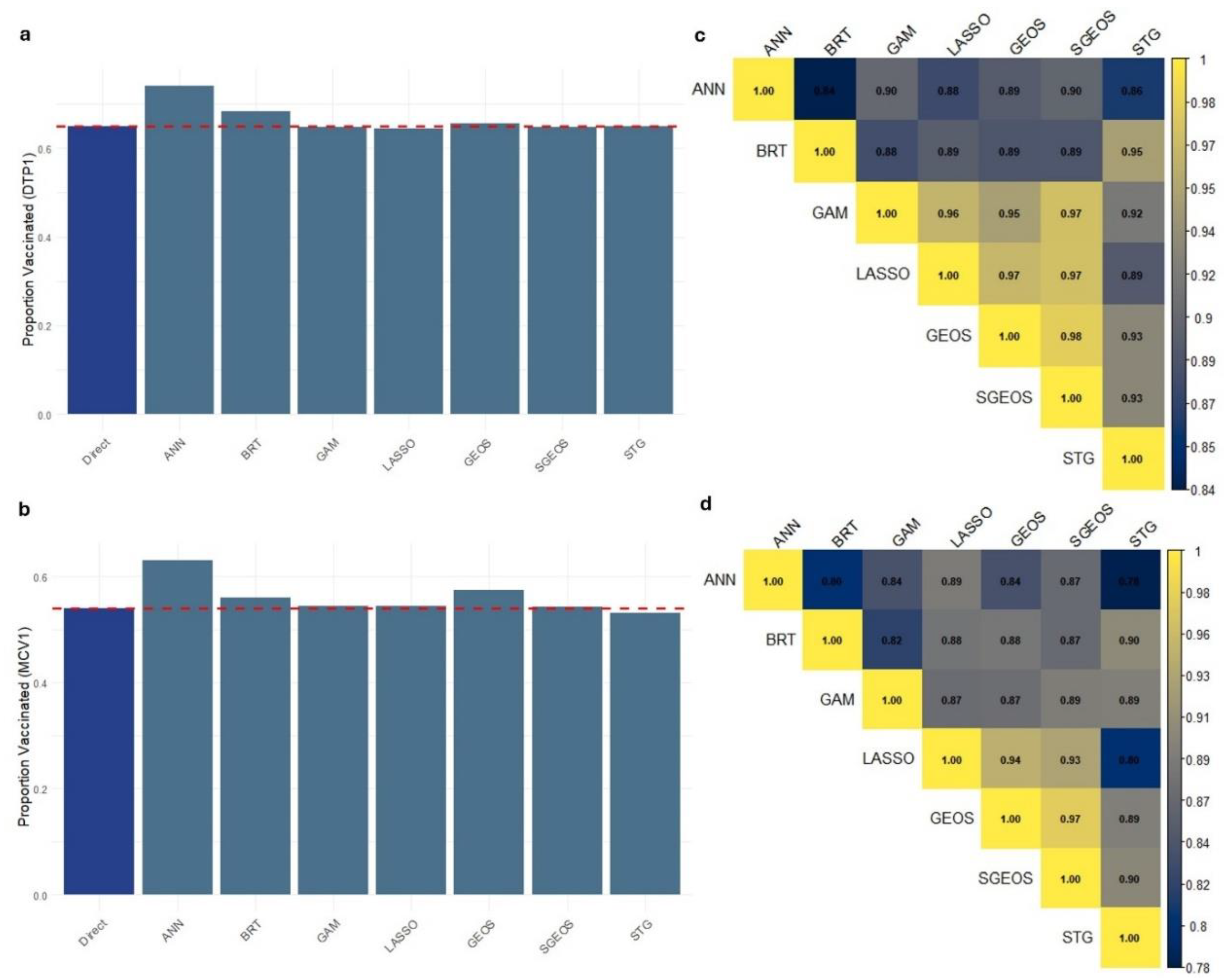
At the national level, the estimates produced through using these approaches revealed that ANN (and BRT to some extent; and GEOS – MCV1 only) overestimated coverage for both DTP1 and MCV1 relative to the direct survey estimate that is often considered to be the gold standard (
Figure 6a,b). On the other hand, whilst there are strong correlations between the grid level estimates produced by these approaches (
Figure 6c,d), it is evident that ANN and BRT are most dissimilar to other approaches, particularly for DTP1.
3.3. Exploring Spatial Prioritization Using District Level Coverage Estimates
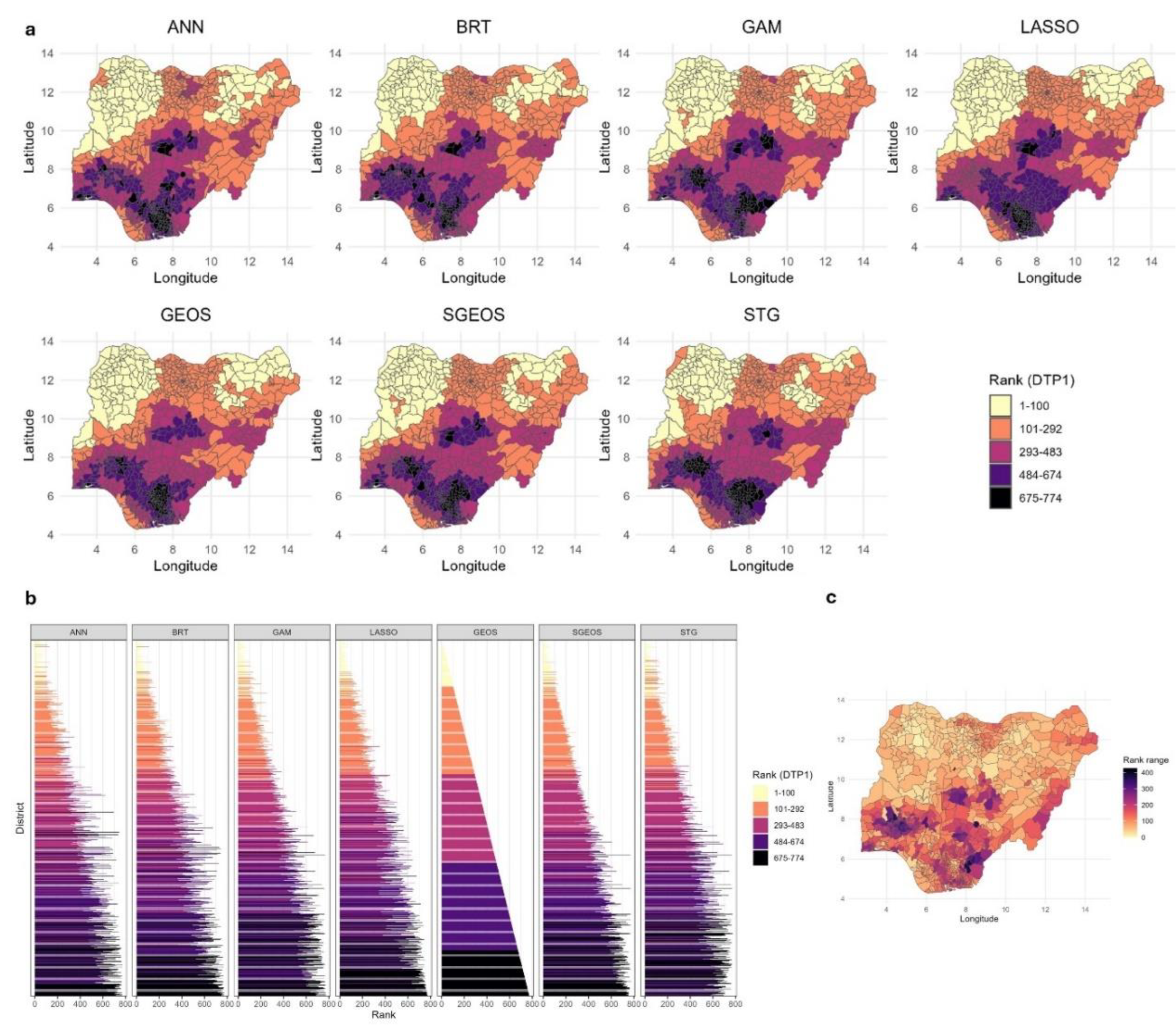
To further investigate the utility of the coverage estimates produced by the methods for spatial prioritization, we computed district level coverage estimates using their respective 1x1 km predicted maps and then ranked the districts based on these estimates. We note that the comparisons undertaken here using rankings obtained from the district-level coverage estimates are purely for illustration since estimates of numbers of unvaccinated children can characterise disease risk more accurately and are better suited for this purpose.
Figure 7 (a-c) demonstrate that although there are broad similarities between the rankings of the district level DTP1 coverage estimates produced by the different methods, remarkable differences exist, both when examining groups of ranks (
Figure 7a) and, more evidently, the individual ranks (
Figure 7b). The differences between the rankings generally appear relatively smaller in areas of lower coverage in the northern parts of the country and much larger in higher coverage areas (
Figure 6c). Also, these differences appear more pronounced when considering smaller numbers of areas (e.g., the 80th to 100thlowest coverage areas) than larger numbers of areas (e.g., the 100 lowest coverage areas) (
Figure 7b). The median of the ranges of the ranks per district (
Figure 7c) at the national level is 112.5 (interquartile range (IQR) = 100, maximum value = 428), indicating marked differences among the methods. Among the five methods with similar predictive performance (i.e., GAM, LASSO, GEOS, SGEOS and STG), the median of the ranges of the ranks per district reduces to 83 (IQR = 89, maximum value = 337), which still indicates considerable differences. However, when examining pairs of methods with more similar predictive accuracy, there were large reductions in the differences between the rankings. For example, for the GEOS and SGEOS methods, the median of the ranges of the ranks per district is 17 (IQR=32).
Similar patterns were observed for MCV1 (supplementary Figure S14), with the median of the ranges of the ranks per district estimated to be 141 (IQR=114, maximum value = 499) for all the methods at the national level, 87 (IQR=82, maximum value = 336) for GAM, LASSO, GEOS, SGEOS and STG, and 26 (IQR=50) for the GEOS and SGEOS methods. These differences in the rankings produced by the methods are also apparent in the bivariate plots of the ranks shown in supplementary Figures S15 and S16.
4. Discussion
For the first time, our study evaluated the performance of seven geostatistical and ML approaches for producing estimates of vaccination coverage at resolved spatial scales. All the methods were implemented using standard computers with a maximum run time of < 3 hours per method needed (much lower for some ML approaches) to produce predictions at 1x1 km resolution, except the SGEOS method which was executed using a high memory computer with a run time of 2.5 hours.
Our analyses revealed similar out-of-sample predictive performance at the cluster level for five of the methods - GEOS, SGEOS, LASSO, GAM and STG, although stronger predictive performance was observed for GEOS, SGEOS and LASSO methods. Out of all seven approaches investigated, ANN and BRT had the worst predictive performance. The over-smoothing observed in both approaches relative to others can be due to the way their algorithms learn from data or the different outcome distribution (Gaussian instead of binomial) used for both approaches. We observed that it did not matter which group of covariates were used to predict coverage when using both approaches, e.g., kriged DHS covariates and other geospatial covariates, as the over-smoothing persisted in both cases – see supplementary Figure S17. Interestingly, when considering the Bayesian approaches, we found that GEOS and SGEOS generally outperformed the STG method, despite the extensive use of the latter approach for producing gridded estimates of HDIs (Bhatt et al., 2017, Mosser et al., 2019, Sbarra et al., 2021). These results were further corroborated when examining the in-sample predictions from the methods for residual spatial autocorrelation and when comparing their out-of-sample predictions in low coverage areas. We did not find evidence of better predictive performance for MCV1 due to greater cluster level sample sizes relative to DTP1. This is likely due to the sample sizes for MCV1 not being large enough to make a difference. The effect of cluster-level sample sizes on in- and out-of-sample predictive performance is well explored in Utazi et al (Utazi et al., 2022).
The 1x1 km predicted maps of the indicators revealed that while GAM, LASSO, GEOS, SGEOS and STG produced very similar results, ANN and BRT produced grid level estimates that were over-smoothed relative to the other approaches, with the estimates being close to the endpoints of the coverage scale. Although the uncertainties produced by these approaches had very similar spatial distributions, the uncertainties for ANN and BRT were either relatively smaller (for DTP1)– an artefact of the binomial distribution and over-smoothing – or appeared relatively noisier in some areas and relatively higher (for MCV1) than those of the other approaches. The correlations between the grid level estimates produced by the approaches are generally high (), but these also indicated relatively lower correlations between ANN and BRT and other approaches, particularly for DTP1. Further comparisons with direct survey estimates at the national level revealed that ANN consistently overestimated coverage. There was also some evidence of overestimation by BRT. We note that given the differences between the predictions obtained through using ANN and BRT and other approaches, both ANN and BRT approaches are also likely to produce other subnational estimates (e.g., at the provincial level) that do not align well with direct survey estimates.
Considering the importance of district level estimates of vaccination coverage and corresponding estimates of numbers of zero-dose and under-vaccinated children for program planning and implementation, we further investigated the utility of the coverage estimates produced by the different approaches for spatial prioritization at the district level. We found remarkable differences in their rankings of the districts, although there were broad similarities especially when considering larger numbers of areas. The differences in the ranks per district seemed greatest in areas of higher coverage and more modest in lower coverage areas, which might have been affected by the spatial distribution of vaccination coverage in the study country. We further observed a reduction in differences in rankings among methods with similar predictive performance, as expected, and even substantial reductions between pairs of methods with similar predictive performance. These results hold significant implications for vaccination programming, especially in resource-constrained settings where only a limited number of areas can be targeted per time, since inaccurate identification of priority areas for interventions could result in missing important vulnerable populations, suboptimal resource allocation, reduced impact and persistence of disease circulation and outbreaks. The predictive accuracy of these approaches should therefore guide their use for map production and operationalization.
Although our study is the first of its kind in relation to vaccination coverage estimation, our findings are broadly consistent with those of other studies that compared geostatistical and ML approaches in other applications such as air pollution (Berrocal et al., 2020) and soil organic carbon mapping (Veronesi and Schillaci, 2019), which also found that geostatistical models outperformed ML approaches. However, our results are somewhat different from those of Bosco et al (Bosco et al., 2017) who used ANN and a Bayesian geostatistical model to map various HDIs across multiple countries and found that both approaches had very similar predictive performance, with the latter being the preferred approach due to ease of implementation (i.e., not requiring many tuning parameters). This may be due to differences in study design and geography, model implementation choices including parameter tuning, the cross-validation approaches used, the nature of the outcome indicators or the geospatial covariates included in both studies, which make direct comparisons of the results less tenable.
There are a number of factors that underlie the results obtained in our study. Our data were taken from a specific geography. It will be useful to explore how these methods perform in other settings with different sampling designs and spatial distributions of vaccination coverage, although we investigated the latter to some degree by considering two indicators of vaccination coverage. Also, other factors that can potentially influence the comparisons of these methods are varying levels of spatial autocorrelation in the outcome data and varying numbers and types of covariates included in the model and their relationships with vaccination coverage (Bosco et al., 2017). The underperformance observed in ANN and BRT may depend on some of these factors, since ML approaches rely on covariates to make predictions whilst the geostatistical approaches additionally leverage residual spatial autocorrelation, but it also reveals a lack of robustness of both approaches to some modelling contexts. For geostatistical models, these attributes have been investigated in detail in previous work using simulation studies (e.g., Utazi et al (Utazi et al., 2018a)) . However, we would like to clarify that a simulation study would only be ideal when comparing only geostatistical models such as the GEOS, SGEOS and STG models investigated here, since simulating data from a geostatistical model or a sampling design based on geostatistical techniques would confer an undue advantage on these models over ML techniques. It will also be interesting to investigate the performance of these approaches in scenarios where the survey is representative at the district or the second administrative level, although the relevance of the modelled estimates is weakened in this case. Furthermore, other approaches for estimating the uncertainties associated with the ML approaches are also possible. For example, a spatial bootstrap algorithm (this did not perform well in our study during initial trials) or an approach that involves interpolating spatial cross-validation residuals to create an uncertainty map, similar to Blanco et al (Guio Blanco et al., 2018), could be used.
Whilst the use of geostatistical and ML approaches to produce high-resolution maps of HDIs has grown in popularity, other small area estimation methods for producing maps of HDIs exist (Tzavidis et al., 2018, Utazi et al., 2021, Paige et al., 2022), but these assume a discrete spatial domain, meaning that estimates can only be produced for a given administrative level at a time. Some of these methods are well explored in Utazi et al (Utazi et al., 2021). Furthermore, in the ML arena, there are other hybrid approaches aiming to overcome the limitation of ML approaches not explicitly accounting for spatial autocorrelation in the data through (i) creating features that imitate the spatial autocorrelation in the outcome and using these as additional covariates in conventional ML methods (Sekulić et al., 2020, Fouedjio and Arya, 2024), (ii) combining ML predictions with the kriging of the prediction residuals (Kaya et al., 2022) and (iii) locally calibrated ML algorithms (Hagenauer and Helbich, 2022, Fouedjio and Arya, 2024). Future work in mapping vaccination coverage and other HDIs may involve the exploration of these hybrid approaches. In geostatistical models, spatially varying coefficient models (Gelfand et al., 2003) can also be used to account for the spatial non-stationarity in the regression relationship between vaccination coverage and geospatial covariate information.
In conclusion, our results provide valuable guidance to practitioners regarding the utility of these modelling approaches for producing maps of vaccination coverage and other HDIs. While most of the approaches we investigated had good predictive accuracy and produced similar results, some approaches were relatively better, with significant implications for spatial prioritization. Effort should be made to either identify the best modelling framework for each analytical context or to use approaches that have been shown to be more robust and reliable in other contexts.
Author Contributions
CRediT: C. Edson Utazi: Conceptualization, Data Curation, Methodology, Formal analysis, Software, Supervision, Visualization, Funding acquisition, Writing – original draft, Writing – review and editing. Ortis Yankey: Data Curation, Methodology, Formal analysis, Software, Writing – review and editing. Somnath Chaudhuri: Data Curation, Methodology, Formal analysis, Software, Visualization, Writing – original draft, Writing – review and editing. Iyanuloluwa D. Olowe: Data Curation, Writing – review and editing. M. Carolina Danovaro-Holliday: Conceptualization, Writing – review and editing. Attila N. Lazar: Supervision, Funding acquisition, Writing – review and editing. Andrew J. Tatem: Supervision, Funding acquisition, Writing – review and editing.
Funding
CEU, ANL and AJT were supported by funding from Gavi, the Vaccine Alliance. CEU, SC and ANL were supported by funding from UNICEF (Grant number: 43387656).
Ethical approval
The study utilized anonymized secondary data. Ethics approval was provided by the University Ethics Committee (Application ID: 48522.A1), University of Southampton, UK.
Data and code availability
All the data used in the study are available from the sources referenced in the manuscript. The authors do not have the rights to redistribute these data. All R code used in the analyses is available via GitHub
https://github.com/EdsonUtazi/GEOS_ML_paper.
Acknowledgements
The authors would like to thank the VaxPop Project team for their support during the study.
Competing interests
The authors declare that they have no known competing financial interests or personal relationships that could have appeared to influence the work reported in this paper. MCD-H works at the World Health Organisation. The comments on this article reflect those of the authors alone and do not necessarily reflect those of the World Health Organization.
References
- Aheto, J. M. K., Olowe, I. D., Chan, H. M., Ekeh, A., Dieng, B., Fafunmi, B., Setayesh, H., Atuhaire, B., Crawford, J., Tatem, A. J. & Utazi, C. E. 2023. Geospatial analyses of recent household surveys to assess changes in the distribution of zero-dose children and their associated factors before and during the covid-19 pandemic in nigeria. Vaccines, 11. [CrossRef]
- Alegana, V. A., Ticha, J. M., Mwenda, J. M., Katsande, R., Gacic-Dobo, M., Danovaro-Holliday, M. C., Shey, C. W., Akpaka, K. A., Kazembe, L. N. & Impouma, B. 2024. Modelling the spatial variability and uncertainty for under-vaccination and zero-dose children in fragile settings. Scientific Reports, 14, 24405. [CrossRef]
- Berrocal, V. J., Guan, Y., Muyskens, A., Wang, H., Reich, B. J., Mulholland, J. A. & Chang, H. H. 2020. A comparison of statistical and machine learning methods for creating national daily maps of ambient pm2.5 concentration. Atmospheric Environment, 222, 117130. [CrossRef]
- Bhatt, S., Cameron, E., Flaxman, S. R., Weiss, D. J., Smith, D. L. & Gething, P. W. 2017. Improved prediction accuracy for disease risk mapping using gaussian process stacked generalization. Journal of The Royal Society Interface, 14, 20170520. [CrossRef]
- Bosco, C., Alegana, V., Bird, T., Pezzulo, C., Bengtsson, L., Sorichetta, A., Steele, J., Hornby, G., Ruktanonchai, C., Ruktanonchai, N., Wetter, E. & Tatem, A. J. 2017. Exploring the high-resolution mapping of gender-disaggregated development indicators. Journal of The Royal Society Interface, 14, 20160825. [CrossRef]
- Browne, C., Matteson, D. S., Mcbride, L., Hu, L., Liu, Y., Sun, Y., Wen, J. & Barrett, C. B. 2021. Multivariate random forest prediction of poverty and malnutrition prevalence. PLOS ONE, 16, e0255519. [CrossRef]
- Chopra, M., Bhutta, Z., Chang Blanc, D., Checchi, F., Gupta, A., et al. 2020. Addressing the persistent inequities in immunization coverage. Bull World Health Organ, 98, 146-148. [CrossRef]
- Croft, T. N., Allen, C. K. & Zachary, B. W. 2023. Guide to dhs statistics. Rockville, Maryland, USA: ICF.
- Diggle, P. J., Tawn, J. A. & Moyeed, R. A. 1998. Model-based geostatistics. Journal of the Royal Statistical Society Series C: Applied Statistics, 47, 299-350.
- Dong, T. Q. & Wakefield, J. 2021. Modeling and presentation of vaccination coverage estimates using data from household surveys. Vaccine, 39, 2584-2594. [CrossRef]
- Dowell, S. F., Blazes, D. & Desmond-Hellmann, S. 2016. Four steps to precision public health. Nature, 540, 189-191.
- Fouedjio, F. & Arya, E. 2024. Locally varying geostatistical machine learning for spatial prediction. Artificial Intelligence in Geosciences, 5, 100081. [CrossRef]
- Friedman, J., Hastie, T., Tibshirani, R., Narasimhan, B., Tay, K., Simon, N. & Qian, J. 2021. Package ‘glmnet’. CRAN R Repositary, 595.
- Fryda, T., Ledell, E., Gill, N., Aiello, S., Fu, A., Candel, A., Click, C., Kraljevic, T. & Nykodym, T. 2024. R package ‘h2o’: R interface for the 'h2o' scalable machine learning platform.
- Fuglstad, G.-A., Simpson, D., Lindgren, F. & Rue, H. 2019. Constructing priors that penalize the complexity of gaussian random fields. Journal of the American Statistical Association, 114, 445-452. [CrossRef]
- Gascoigne, C., Smith, T., Paige, J. & Wakefield, J. 2025. Estimating subnational under-five mortality rates using a spatio-temporal age-period-cohort model. Spatial and Spatio-temporal Epidemiology, 52, 100708. [CrossRef]
- Gavi the Vaccine Alliance. 2020. Gavi strategy 5.0, 2021-2025. Available: https://www.gavi.org/our-alliance/strategy/phase-5-2021-2025 [Accessed 25 June 2021].
- Gelfand, A. E., Kim, H.-J., Sirmans, C. F. & Banerjee, S. 2003. Spatial modeling with spatially varying coefficient processes. Journal of the American Statistical Association, 98, 387-396. [CrossRef]
- Guio Blanco, C. M., Brito Gomez, V. M., Crespo, P. & Ließ, M. 2018. Spatial prediction of soil water retention in a páramo landscape: Methodological insight into machine learning using random forest. Geoderma, 316, 100-114. [CrossRef]
- Hagenauer, J. & Helbich, M. 2022. A geographically weighted artificial neural network. International Journal of Geographical Information Science, 36, 215-235.
- James, G., Witten, D., Hastie, T. & Tibshirani, R. 2013. An introduction to statistical learning: With applications in r, Spinger.
- Janocha, B., Donohue, R. E., Fish, T. D., Mayala, B. K. & Croft, T. N. 2021. Guidance and recommendations for the use of indicator estimates at subnational administrative level 2. DHS Spatial Analysis Report 20. Rockville, Maryland, USA: ICF.
- Johns, N. E., Hosseinpoor, A. R., Chisema, M., Danovaro-Holliday, M. C., Kirkby, K., Schlotheuber, A., Shibeshi, M., Sodha, S. V. & Zimba, B. 2022. Association between childhood immunisation coverage and proximity to health facilities in rural settings: A cross-sectional analysis of service provision assessment 2013–2014 facility data and demographic and health survey 2015–2016 individual data in malawi. BMJ Open, 12, e061346. [CrossRef]
- Kawakatsu, Y., Mosser, J. F., Adolph, C., Baffoe, P., Cheshi, F., Aiga, H., Watkins, D. A. & Sherr, K. H. 2024. High-resolution mapping of essential maternal and child health service coverage in nigeria: A machine learning approach. BMJ Open, 14, e080135. [CrossRef]
- Kaya, F., Keshavarzi, A., Francaviglia, R., Kaplan, G., Başayiğit, L. & Dedeoğlu, M. 2022. Assessing machine learning-based prediction under different agricultural practices for digital mapping of soil organic carbon and available phosphorus. Agriculture, 12, 1062. [CrossRef]
- Kinyoki, D. K., Osgood-Zimmerman, A. E., Pickering, B. V., Schaeffer, L. E., Marczak, L. B., et al. 2020. Mapping child growth failure across low- and middle-income countries. Nature, 577, 231-234.
- Lim, S. S., Stein, D. B., Charrow, A. & Murray, C. J. L. 2008. Tracking progress towards universal childhood immunisation and the impact of global initiatives: A systematic analysis of three-dose diphtheria, tetanus, and pertussis immunisation coverage. The Lancet, 372, 2031-2046. [CrossRef]
- Lindgren, F., Bachl, F., Illian, J., Suen, M. H., Rue, H. & Seaton, A. E. 2024. Inlabru: Software for fitting latent gaussian models with non-linear predictors. arXiv preprint arXiv:2407.00791.
- Lindgren, F., Rue, H. & Lindström, J. 2011. An explicit link between gaussian fields and gaussian markov random fields: The stochastic partial differential equation approach. J Roy Stat Soc Series B (Stat Methodol), 73, 423-498. [CrossRef]
- Lindgren, F., Rue, H. & Lindström, J. 2015. Bayesian spatial modelling with r-inla. Journal of Statistical Software, 63, 25. [CrossRef]
- Matérn, B. 1960. Spatial variation, Berlin, Germany, Springer-Verlag.
- Mayala, B., Dontamsetti, T., Fish, T. & Crof, T. 2019. Interpolation of dhs survey data at subnational administrative level 2. Dhs spatial analysis reports no. 17. Rockville: ICF. [CrossRef]
- Mosser, J. F., Gagne-Maynard, W., Rao, P. C., Osgood-Zimmerman, A., Fullman, N., et al. 2019. Mapping diphtheria-pertussis-tetanus vaccine coverage in africa, 2000 - 2016: A spatial and temporal modelling study. The Lancet, 393, 1843-1855. [CrossRef]
- Mwinnyaa, G., Hazel, E., Maïga, A. & Amouzou, A. 2021. Estimating population-based coverage of reproductive, maternal, newborn, and child health (rmnch) interventions from health management information systems: A comprehensive review. BMC Health Services Research, 21, 1083. [CrossRef]
- National Population Commission - Npc & Icf 2019. Nigeria demographic and health survey 2018 - final report. Abuja, Nigeria: NPC and ICF.
- Nychka, D., Furrer, R., Paige, J. & Sain, S. 2017. Fields: Tools for spatial data. R package version, 9, D6W957CT.
- Paige, J., Fuglstad, G.-A., Riebler, A. & Wakefield, J. 2022. Design- and model-based approaches to small-area estimation in a low- and middle-income country context: Comparisons and recommendations. Journal of Survey Statistics and Methodology, 10, 50-80. [CrossRef]
- Park, Y. S. & Lek, S. 2016. Chapter 7 - artificial neural networks: Multilayer perceptron for ecological modeling. In: JØRGENSEN, S. E. (ed.) Developments in environmental modelling. Elsevier.
- Perez-Haydrich, C., Warren, J. L., Burgert, C. R. & Emch, M. E. 2013. Guidelines on the use of dhs gps data. DHS Spatial Analysis Reports No. 8. Calverton, Maryland, USA: ICF International.
- R Core Team 2021. A language and environment for statistical computing. Vienna, Austria.
- Rao, J. N. 2005. Small area estimation, John Wiley & Sons.
- Ribeiro Jr, P. J., Diggle, P. J., Christensen, O., Schlather, M., Bivand, R. & Ripley, B. 2024. The geor package: Analysis of geostatistical data.
- Ridgeway, G. & Ridgeway, M. G. 2004. The gbm package. R Foundation for Statistical Computing, Vienna, Austria, 5.
- Sbarra, A. N., Rolfe, S., Nguyen, J. Q., Earl, L., Galles, N. C., et al. 2021. Mapping routine measles vaccination in low- and middle-income countries. Nature, 589, 415-419. [CrossRef]
- Scobie, H. M., Edelstein, M., Nicol, E., Morice, A., Rahimi, N., Macdonald, N. E., Carolina Danovaro-Holliday, M. & Jawad, J. 2020. Improving the quality and use of immunization and surveillance data: Summary report of the working group of the strategic advisory group of experts on immunization. Vaccine, 38, 7183-7197. [CrossRef]
- Sekulić, A., Kilibarda, M., Heuvelink, G. B., Nikolić, M. & Bajat, B. 2020. Random forest spatial interpolation. Remote Sensing, 12, 1687. [CrossRef]
- Shattock, A. J., Johnson, H. C., Sim, S. Y., Carter, A., Lambach, P., et al. 2024. Contribution of vaccination to improved survival and health: Modelling 50 years of the expanded programme on immunization. The Lancet, 403, 2307-2316. [CrossRef]
- Simpson, D., Rue, H., Riebler, A., Martins, T. G. & Sørbye, S. H. 2017. Penalising model component complexity: A principled, practical approach to constructing priors. [CrossRef]
- Takahashi, S., Metcalf, C. J. E., Ferrari, M. J., Tatem, A. J. & Lessler, J. 2017. The geography of measles vaccination in the african great lakes region. Nature Communications, 8, 15585. [CrossRef]
- Tatem, A. J. 2017. Worldpop, open data for spatial demography. Scientific Data, 4, 170004. [CrossRef]
- Tzavidis, N., Zhang, L.-C., Luna, A., Schmid, T. & Rojas-Perilla, N. 2018. From start to finish: A framework for the production of small area official statistics. Journal of the Royal Statistical Society Series A: Statistics in Society, 181, 927-979. [CrossRef]
- UNICEF and the Bill and Melinda Gates Foundation. 2021. Equity reference group for immunization advocacy brief. Available: https://drive.google.com/file/d/1VpuVX85RWd_vq6FJ4lcmCnPOYJp1AhuM/view [Accessed 05 May 2021].
- United Nations. 2015. Transforming our world: The 2030 agenda for sustainable development. Available: http://www.un.org/ga/search/view_doc.asp?symbol=A/RES/70/1&Lang=E [Accessed 20 June 2017].
- Utazi, C. E., Aheto, J. M. K., Chan, H. M. T., Tatem, A. J. & Sahu, S. K. 2022. Conditional probability and ratio-based approaches for mapping the coverage of multi-dose vaccines. Statistics in Medicine, 41, 5662 - 5678. [CrossRef]
- Utazi, C. E., Aheto, J. M. K., Wigley, A., Tejedor-Garavito, N., Bonnie, A., Nnanatu, C. C., Wagai, J., Williams, C., Setayesh, H., Tatem, A. J. & Cutts, F. T. 2023. Mapping the distribution of zero-dose children to assess the performance of vaccine delivery strategies and their relationships with measles incidence in nigeria. Vaccine, 41, 170-181. [CrossRef]
- Utazi, C. E., Nilsen, K., Pannell, O., Dotse-Gborgbortsi, W. & Tatem, A. J. 2021. District-level estimation of vaccination coverage: Discrete vs continuous spatial models. Stat Med, 40, 2197-2211. [CrossRef]
- Utazi, C. E., Thorley, J., Alegana, V. A., Ferrari, M. J., Nilsen, K., Takahashi, S., Metcalf, C. J. E., Lessler, J. & Tatem, A. J. 2018a. A spatial regression model for the disaggregation of areal unit based data to high-resolution grids with application to vaccination coverage mapping. Statistical Methods in Medical Research, 28, 3226-3241. [CrossRef]
- Utazi, C. E., Thorley, J., Alegana, V. A., Ferrari, M. J., Takahashi, S., Metcalf, C. J. E., Lessler, J., Cutts, F. T. & Tatem, A. J. 2019. Mapping vaccination coverage to explore the effects of delivery mechanisms and inform vaccination strategies. Nature Communications, 10, 1633. [CrossRef]
- Utazi, C. E., Thorley, J., Alegana, V. A., Ferrari, M. J., Takahashi, S., Metcalf, C. J. E., Lessler, J. & Tatem, A. J. 2018b. High resolution age-structured mapping of childhood vaccination coverage in low and middle income countries. Vaccine, 36, 1583-1591. [CrossRef]
- Veronesi, F. & Schillaci, C. 2019. Comparison between geostatistical and machine learning models as predictors of topsoil organic carbon with a focus on local uncertainty estimation. Ecological Indicators, 101, 1032-1044. [CrossRef]
- Wahba, G. 1981. Spline interpolation and smoothing on the sphere. SIAM Journal on Scientific and Statistical Computing, 2, 5-16.
- Wang, L. & Yu, F. 2021. Jackknife resample method for precision estimation of weighted total least squares. Communications in Statistics - Simulation and Computation, 50, 1272-1289. [CrossRef]
- Wang, X., Yue, Y. R. & Faraway, J. J. 2018. Bayesian regression modeling with inla, Chapman and Hall/CRC.
- Weiss, D. J., Lucas, T. C. D., Nguyen, M., Nandi, A. K., Bisanzio, D., et al. 2019. Mapping the global prevalence, incidence, and mortality of plasmodium falciparum, 2000-17: A spatial and temporal modelling study. The Lancet, 394, 322-331.
- Wigley, A., Lorin, J., Hogan, D., Utazi, C. E., Hagedorn, B., Dansereau, E., Tatem, A. J. & Tejedor-Garavito, N. 2022. Estimates of the number and distribution of zero-dose and under-immunised children across remote-rural, urban, and conflict-affected settings in low and middle-income countries. PLOS Global Public Health, 2, e0001126. [CrossRef]
- Wood, S. & Wood, M. S. 2015. Package ‘mgcv’. R package version, 1, 729.
- Wood, S. N. 2011. Fast stable restricted maximum likelihood and marginal likelihood estimation of semiparametric generalized linear models. Journal of the Royal Statistical Society Series B: Statistical Methodology, 73, 3-36. [CrossRef]
- World Health Organization. 2018. World health organization vaccination coverage cluster surveys: Reference manual. Available: https://apps.who.int/iris/handle/10665/272820.
- World Health Organization. 2020. Immunization agenda 2030: A global strategy to leave no one behind. Available: https://www.who.int/immunization/immunization_agenda_2030/en/ [Accessed 25/06/2020].
|
Disclaimer/Publisher’s Note: The statements, opinions and data contained in all publications are solely those of the individual author(s) and contributor(s) and not of MDPI and/or the editor(s). MDPI and/or the editor(s) disclaim responsibility for any injury to people or property resulting from any ideas, methods, instructions or products referred to in the content. |
© 2024 by the authors. Licensee MDPI, Basel, Switzerland. This article is an open access article distributed under the terms and conditions of the Creative Commons Attribution (CC BY) license (http://creativecommons.org/licenses/by/4.0/).