
Submitted:
24 December 2024
Posted:
25 December 2024
You are already at the latest version
Abstract
RNA inverse design is an essential part of many RNA therapeutics strategies. To date, there have been great advances in the computationally-driven RNA design. Current machine-learning approaches can predict the sequence of an RNA given its 3D structure with acceptable accuracy and tremendous speed. Design and engineering of RNA regulators such as riboswitches, however, is often more difficult, partly due to their inherent conformational switching abilities. Although recent state-of-the-art models do incorporate information about the multiple structures a sequence can fold into, there is great room for improvement in modeling structural switching. In this work, a relational geometric graph neural network is proposed that explicitly incorporates alternative structures to predict the RNA sequence. The proposed model uses edge types to distinguish primary-, secondary-, and tertiary-structure pairing/positioning of nucleotides for its training. Results show higher native sequence recovery rates over gRNAde across different test sets (eg. 72% vs 66%) and a benchmark from the literature (60% vs 57%). The impact of secondary-structure on prediction accuracy was more significant than that of tertiary-structure dependencies as defined here. The code for the above relational GNN can be found here.
Keywords:
RNA inverse design
; geometric deep learning
; riboswitches
; graph neural networks
1. Introduction
RNA molecule design is essential to gene therapy, drug development, biosensing, synthetic biology, and more recently, mRNA vaccines[1,2,3]. However, in deep learning explorations, protein sequence-structure analyses have enjoyed more advances than RNAs. These advances are partly due to the significant amount of available data on protein structures [4,5,6,7,8]. Apart from the paucity of data, other major factors posing challenges in RNA inverse design are RNA’s inherent flexibility, plasticity, in some cases its ability to form distinct conformations under different environmental factors, and non-unique structure-sequence mapping.
Structure-based design of RNAs capable of folding into alternative structures, known as RNA switches or riboswitches [9] is of great interest in biotechnology and therapeutics [10]. Probably representatives of an ancient regulatory mechanism [11,12] even long before proteins [13,14,15,16] riboswitches are usually located in the 5’ untranslated region (UTR) of an mRNA. They generally consist of a ligand-binding aptamer that upon binding to the ligand or metabolite of interest can allosterically alter the structure of the rest of the riboswitch which also includes an expression platform, in turn regulating transcription or translation of downstream genes in bacteria [9,17,18,19]. Currently categorized into 55 distinct classes, riboswitches enjoy a great structural and functional diversity [20,21,22] as well as the diversity of ligands that bind to them helping cells regulate a great variety of chemicals essential to all forms of life [18,23]. It is speculated that additional classes of riboswitches exist in not only bacteria but also eukaryotes [16,18]. Riboswitches are used in many therapeutic and biotechnological applications including Riboswitch-targeting antibiotics [24,25,26,27], designer gene control [28,29,30], molecular fuse [31,32], and research tools to explore fundamental biological processes [33].
RNA inverse design has been traditionally based on RNA’s 2D or secondary structure [34]. More recent approaches such as libLEARNA [35] incorporate sequence and secondary-structure constraints to to perform partial sequence design with outstanding performance applied on riboswitches. One of the more popular 2D inverse folding tools is ViennaRNA [36], which predicts the complete sequence.
RNA computational design directly from its 3D structure can be performed by the state-of-the-art physically based molecular modeling software Rosetta [37]. Several deep learning approaches to 3D RNA inverse design have been explored in the past few years that are based on Graph Neural Network (GNN) architectures. Some of these methods are the representation-based learning approach RDesign [38] and the diffusion model RiboDiffusion [39] that uses a Transformer-based sequence module. Another GNN-based model, gRNAde [40], which incorporates concepts from autoregressive GVP-GNN [41] and protein sequence design ProteinMPNN [6] has been shown to achieve a higher native sequence recovery compared to Rosetta and RDesign on a set of benchmark sequences that include riboswitches and ribozymes [42]. The multi-state architecture of gRNAde software uses multiple structures of a single sequence in its training and design. The architectural design, however, is more geared towards aggregating multiple structural information, rather than combining them, which could lead to loss of information in certain cases. An approach that is based on combining information from multiple structural states, however, is yet to be fully explored. In this work, based on gRNAde, a secondary-structure-informed relational Graph Neural Network (GNN) is proposed for RNA inverse design with an architecture that emphasizes learning from RNAs specifically having distinct alternative structures, i.e., riboswitches. The model uses geometric-vector-perception GNN [41] layers and has a similar architecture to gRNAde [40,43], with the following alterations:
The edge embedding does not include 16 sinusoidal positional encodings. In addition, edges consist of three different types: Primary-structure edge types, secondary-structure edge types, and tertiary-structure edge types. Primary-structure edge types are defined along the sequence backbone. Secondary-structure edge types are determined by an independent software [44,45] that detects canonical and non-canonical RNA base pairing. Tertiary-structure edge types here have a specific definition and are based on clustering nucleotides based on a combination of their backbone and Euclidean distances. An example of edge types is illustrated in Figure 1, which corresponds to a section of the immature 30S ribosomal subunit of Staphylococcus aureus. Details about edge determination are explained in Materials and Methods. Each encoder layer consists of three distinct GVP-GNNs, one for each edge type. Finally, the decoder takes updated node embeddings of the last layer of the encoder, each resulting from a distinct structural scenario that the sequence can fold into, pooling them to produce the final updated node embedding. The proposed relational GNN is also -equivariant and message-passing components are implemented via PyTorch Geometric [46]. The Materials and Methods section describes details about input embedding and model architecture.
The paper first defines model architecture in Materials and Methods. In the Results section, the performance of the relational GNN is then presented and compared to their corresponding gRNAde counterparts under different data splits and model variations. Finally, the Discussion section contains conclusions drawn from performance analyses and future direction.
2. Materials and Methods
2.1. Data Collection
RNA structure files were downloaded from the RNASolo [48] repository on August 1, 2024. There were a total of 14,889 PDB files at resolution Å. The cleaned dataset contained a total of 12091 structures, corresponding to 3963 unique sequences. Sequence types were: 2612 Protein-RNA Complexes, 479 Solo RNAs, 14 DNA-RNA Hybrids, and 858 unknowns. Sequence average length was . Only one structure was available for most sequences and the number of structures per sequence followed an exponential distribution with an average value of 3 structures per sequence. In Figure 2, parts (a) and (b) show the distributions of the sequence length and the number of structures per sequence, respectively. Similarity between structures of the same sequence was assessed by computing the average pairwise Root Mean Square Deviation (RMSD) of structures belonging to that sequence. The average value was around 1.3Å. Complete data statistics and histograms can be generated via notebooks/data_stats.ipynb. A machine-learning ready set was then produced based on the downloaded PDB files. In cases of more than one structure in the PDB file, the first one was used. Structures corresponding to the same RNA sequence were then categorized together, representing a multiple-structure single-sequence set of data (see the data availability section for the location of processed files).
2.2. Data Splits
RNA sequences were split into training, validation, and test sets. The sizes of validation and test sets were 100 each. Two different strategies were used to split the data into training and test sets. The first one was denoted as seqid. In this procedure, the aim was to avoid exposing the model to more sequences during training. This was achieved by making the training set have less diverse sequences than the test set. RNA sequences were clustered into groups based on sequence identity using command CD-HIT [49] (threshold 90%) and those with less intra-sequence RMSD among their structures were favored for the training set. In the second strategy, the aim was to avoid exposing the model to more structures during training. This was achieved by making the training set have less diverse structures than the test set. RNA sequences were clustered into groups based on structural similarity using command qTMclust [50] (threshold 0.45%) and those with less intra-sequence RMSD among their structures were favored for the training set. Both data splitting procedures were according to [40].
2.3. Metrics
Performance parameters were perplexity, accuracy, recovery, and sc score. Perplexity reflects the ambiguity within nucleotide probabilities. For instance, a model that predicts equi-probable nucleotides for each node is undesirable. Lower output perplexity is generally favorable1. Accuracy is the ratio of correctly predicted nucleotides. Recovery is the ratio of correctly predicted nucleotides from a population of sequences that are sampled from output probabilities. Here, 16 predictions were used. Similarly, sc score is the secondary-structure self-consistency score averaged over 16 predictions. Software Eternafold [51] was used to measure how well the predicted secondary structures of sampled output sequences match that of the ground-truth sequence.
2.4. Graph Construction of RNA Structures
The 3D coordinates of atoms of an RNA structure, taken from its corresponding PDB file, were used to construct a geometric graph representation (nodes and edges) of the molecule. Three types of edges were defined and denoted as primary-structure , secondary-structure , and tertiary-structure edge types between nodes i and j. Edge types are mutually exclusive: , , .
Nodes
The 3D coordinates for P, C4’, N1 (pyrimidine), or N9 (purine) atoms of each nucleotide were used to define the corresponding node for that nucleotide [52]. The C4’ coordinates of nucleotide i, , represented the 3D coordinates of the corresponding node i. The 3D coordinates of P, C4’, and N1/9 as well as the atoms of the adjacent nucleotides on the RNA backbone were used for feature representation.
Primary-Structure Edge Types
Pairs of consecutive nucleotides on the sequence, i.e., , were assigned primary-structure edge types in both forward and backward directions.
Secondary-Structure Edge Types
Pairs of nucleotides in secondary-structure RNA base pairings, , were assigned secondary-structure edge types. For each base pairing , two edges and were defined. Here, secondary structure base pairings included both canonical and non-canonical pairings [53] and determined by feeding the corresponding PDB file of an RNA to X3dna-dssr [45].
Tertiary-Structure Edge Types
Pairs of nucleotides that did not form secondary structure base pairings but were in close proximity of each other were considered for having what is referred to here as tertiary-structure edge types. The procedure was as follows: Given the secondary-structure base pairs, the unpaired nucleotides were first identified, i.e., , and then clustered using Density-Based Spatial Clustering of Applications with Noise (DBSCAN). Default parameters for DBSCAN were DBSCAN_eps = 20Å and min_samples = 5. Subsequently, those pairs of nucleotides that belonged to the same cluster with distance of DBSCAN_eps, and were also far apart on the RNA sequence were selected. Having distance , or at least 500nt, was considered far apart. i.e., default primary_dist = 500. The number of original tertiary-structure edge types increased exponentially with sequence length. The edges were randomly selected from the original sample, such that the number of tertiary-structure edges was strictly less than or equal to , where L is the length of the corresponding RNA sequence.
The number of edges selected from each RNA molecule is shown in Figure 3). As we can see, the number of edges selected is linear with respect to the length of the sequence. The dashed magenta line shows the cut-off value for cases where the number of original edges was more than the threshold. Edges of RNAs with higher counts were down-sampled to strictly match the threshold.
2.5. Relational Graph Neural Network
Input Embedding
Based originally on [41,54] and identical to the implementation presented in [43], node features were derived from three distances, three inter-atom angles, and three dihedral angles. The number of scalar features associated with each node i was then: sin and cos values of the six angles, concatenated by the three lengths, totaling 15 values. The vector features associated with each node i were four unit vectors corresponding to forward and backward C4’ - P, and forward and backward C4’ - N1/9 vectors. Scalar and vector features of node i are denoted as . Edges of all types, , had identical features. Edge features consisted of both unit vectors and scalar values. Normalized vectors were used as unit vectors. Scalar features consisted of encoded by 16 RBFs. Let represent both scalar and vector features of node i and represent both scalar and vector features of edge . Hence, Let matrix T represent the type of each edge in E in its corresponding indices. For a single sequence-structure scenario, each RNA structure is then represented as a graph . In case of multiple (K) conformations, the graph corresponding to structure k is denoted as . All structures belonging to the same sequence, , are then passed into the GNN model in a single batch. Unlike [40], however, where the K graphs were merged into a single multi-graph with total edges being union of those of individual structures, here edges of each structure k are applied to the model separately. Hence, although the number of nodes is identical amongst the K graphs, the number of edges is not. The rationale behind the above choice of input representation of multiple structures was to favor the expressiveness of an RNA molecule with drastically different conformational states, e.g., a riboswitch, over that of an RNA molecule with only one innate structure but having multiple experimental data on that structure.
Model Encoder
The overall architecture of the pipeline consisted of a linear model, L stacked layers of relational GNNs, and followed by a decoder layer which produces nucleotide probabilities for each sequence location i. Node and edge embeddings are first passed through the linear model. Encoded features are then passed to the first relational GNN layer. The relational GNN consists of three -equivariant GVP-GNN [41] components. Using edge-type indices, T, the encoded features of are first broken down to three sub-graphs, , , and , each representing a graph of a specific edge type. Each of the sub-graph encodings is fed into a separate GVP-GNN (eq. 1), and then pooled using learned weights (eq. 2) to produce updated node features (eq. 3):
Messages with p, s, and t indices reflect primary-structure, secondary-structure, and tertiary-structure messages from neighboring nodes, respectively. Learned weights, reflect the significance of each edge type, i.e., the attention given to different edge types. The above message-passing and pooling mechanism applies to any relational GNN layer and layer indices are omitted for simplicity. For instance, edge-type weights of layer l can be denoted as: . In order to assess the impact of the secondary and tertiary edge types separately, two different versions of the model were used, one including primary and secondary edge types only, denoted by suffix -2D, and one including all edge types, denoted here by suffix -3D.
Scalar and vector node features are updated at every layer (eq. 3). For instance, the output of layer l is . The above message passing scheme is applied to all K structural conformations in the input. At the end of the last encoder layer, the updated node embedding for the k-th structure is . The final node (or nucleotide) embedding given all K structures of the RNA sequence is then an average of individual estimates:
Model Decoder
The original model [40] presented two different decoder implementations: Non-AutoRegressive, NAR-original, and autoregressive AR-original. The NAR-original decoder consisted of two GVP-GNN modules and decoded the node embedding into a dimension of 4 to reflect the four nucleotide probability estimates at each sequence position. The AR-original decoder was an autoregressive model [55] that updated each node embedding based on the nodes there preceded it in the sequence. Here, based on the above two decoders, two secondary-structure-informed decoders by the names NAR-informed and AR-informed were deployed. The implementation of NAR-informed was identical to NAR-original. In the AR-informed decoder, node embeddings specific to structure k are first independently updated, . A final decode layer then pools the individual embeddings to generate final nucleotide probabilities for each sequence position.
3. Results
The proposed RNA inverse design is mainly based on defining different edge types. Unlike primary- and secondary-structure edge types, however, the tertiary-structure edge types are not as deterministic and vary based on the choice of modeling. Here, the intention behind tertiary-structure edges was to capture some of RNA molecule’s tertiary patterns that are evolved beyond the secondary structural constraints. Here, a simple model is used based on the relative orientation of unpaired nucleotides. A general analysis of all the tertiary-structure edge types is provided in A.1. Given the unevenness of the relative-orientation distribution of the unpaired nucleotides (Figure A1 part (a)), it was speculated that introducing tertiary-structure edge types as defined above may contain certain hidden information about RNA nucleotide positioning in 3D space.
The secondary-structure-informed relational GNN architecture use is shown in Figure 4. The model consists of L relational message-passing GNN layers. Each layer pools messages from three distinct GVP-GNN components each corresponding to an edge type. Note that a single GVP-GNN component can be used instead of three where, would be defined as concatenation of , , and . In fact, Eqs (1) and (2) are mathematically equivalent to Equation (1) of [40]. However, since edges are mutually exclusive, the merging of edge types would result in a sparse adjacency matrix. In addition, each vector would have been 3 times an original edge vector, padded by zeros in corresponding locations. Although a single GVP-GNN would have been equivalent to the three original GVP-GNNs, deploying three GVP-GNNs has the advantage of requiring a smaller input size for edges.
Given multiple structures of a particular sequence, each individual sequence-structure pair is fed into the encoder, separately, resulting in a k set of final updated node embeddings (output of layer L). The node embeddings, each resulting from a distinct structure, are then pooled before being fed into the decoder, which produces the final probabilities for each nucleotide i:
Apart from the above re-structuring, The GVP-GNN components, linear, and final decoder layers are adopted from and according to the gRNAde software [40,43]. Two different decoders were introduced in [40] by names one-shot and autoregressive, which are referred to here as NAR-original and AR-original, respectively. Implementations for both models were altered to implement the above secondary-structure-informed relational GNN versions, denoted as NAR-informed and AR-informed, respectively. For each altered implementation, two different versions of *-informed-2D and *-informed-3D were considered. In the case of AR-informed-*, the pooling of updated node embeddings was performed after autoregressive node prediction of individual structure. Hence, eq. (5) holds for all implementations.
Table 1 contains a performance comparison between the original gRNAde and the secondary-structure-informed relational graph neural network under different data split strategies and for different parameters such as the number of encoder layers and inclusion/exclusion of tertiary-structure edge types.
In addition to the [45] software, other choices of software such as Fr3d [56], and corresponding implementation NA_pairwise_interactions.py were considered, which led to similar results (data not shown). The Fr3d software annotates base pair interactions in RNA 3D structures according to the Leontis–Westhof classification [53].
Performance measures of Table 1 were obtained from single runs. Therefore, variation in performance is not available. Based on table (1) of [40], however, we can see that the upper bound of the standard deviation of mean Recovery for is . Since models here are very similar to [40], we assume the mean Recovery to have similar standard deviation measures.
The original autoregressive model AR-original trained on seqid data split, and implemented as part of gRNAde had a lower perplexity as well as higher sc score across all models. Higher sc score is consistent across both sequence-based seqid and tertiary-structure-based structsim data splits.
Comparing models based on accuracy and recovery metrics, however, shows a higher performance for the *-informed-* models compared to their *-original counterparts. The higher performance is true regardless of the choice of data split strategies. In fact, the *-informed-* models only have 2 layers while the original model is set to 4 layers. The comparison here is based on the assumption that the mean Recovery deviation is bounded by . Finally, increasing layers from 2 to 4 further improves the performance of the AR-informed-3D model to recovery=58.37.
Comparing *-informed-2D model performances to their *-informed-3D counterparts shows that tertiary-structure edge types did not result in any major improvement.
Inverse design performance of the seqid-trained AR-informed-3D model was also evaluated on the 14 RNA structures of interest identified by ([42], Supplementary Table 2) and compared to previous methods (See Table 2). Recovery values are based on averaging prediction accuracy over 16 predicted sequences in each case. Our proposed secondary-structure-informed approach had an average of 0.6044 native sequence recovery rate, slightly higher than gRNAde (0.5682) and also higher than other methods including Rosetta (0.45) and RDesign (0.4296). All Recovery values are according to [43].
In order to showcase an example of designing an RNA, an experimentally derived structure of thiamine pyrophosphate (TPP)-sensing riboswitch was selected and passed into the structsim-trained AR-informed-3D model to obtain 16 sequence predictions. The crystal structure of the TPP riboswitch, PDB ID 8F4O, was resolved in the ligand-free (apo) state and with resolution 3.1Å [57]. The sequence with the highest recovery rate (here, 0.7692) was then selected as the final prediction, referred to as Pred_1. Table 3 shows the true and predicted sequences. The structure of Pred_1 was then computationally determined via AlphaFold 3 [58]. AlphaFold provided 5 different predicted structures, the first of which had the highest similarity (lowest RMSD) with the true structure of the TPP riboswitch aptamer. Figure 5 shows the true and predicted structures, in orange and green, respectively. The first and last nucleotides of both structures are shown in licorice mode for ease of visualization. Aligned structures had RMSD of (15.88Å) among all their atoms and RMSD of (16.38Å) among their C4’ atoms. The disconnects in the true structure are due to numbering schemes in the corresponding PDB file. Although the two structures do not have perfect alignment, Figure 5 shows an extended Y-shaped conformation for the predicted structure (green), similar to a typical TPP riboswitch.
4. Discussion and Conclusions
In this work, a geometric GNN-based model was presented to improve the computational design of RNA, especially those with multiple structural states, such as riboswitches. The proposed model named secondary-structure-informed RNA inverse design is mostly taken from gRNAde, with some major differences. These differences were the use of different edge types to represent RNA structural graphs and explicitly combining results from multiple structures in corresponding sequence prediction. Details about these differences are explained in Materials and Methods. It was shown that the proposed model does indeed improve both accuracy and native sequence recovery compared to gRNAde. Using the seqid training/test sets, the autoregressive AR-informed-2D with only two layers obtained 71.12% sequence recovery, while its gRNAde counterpart with four layers produced 66.08% recovery. Similar improvements were seen under the structsim training/test sets (comparing 68.61% with 62.72%) as well as over different choices of decoders (see Table 1). Results demonstrate that the addition of secondary-structure base-pairing information in RNA inverse design and combining predictions via a relational graph architecture does indeed improve performance since both models share similar architectural components and parameters. Improvements may also be due to the fact that identification of canonical and non-canonical base pairings, namely the 12 possible orientations [53], are done independently, relieving the GNN model from the burden of identifying such edges.
Performance of AR-informed-3D was also evaluated on a different benchmark and compared to different methods. The dataset presented in [42] contains 14 structures which include riboswitches and ribozymes. It is shown in Table 2 that the proposed model achieves higher average native sequence recovery on this set over previous methods. The AR-informed model achieved 60.44 native sequence recovery rate, higher than gRNAde (56.82), as well as Rosetta (45) and RDesign (42.96). These results highlight the ability of the proposed approach in the inverse design of novel structures.
4.1. Future Work
In order to identify RNA base pairings, we used X3dna-dssr [45]. Therefore, unlike gRNAde which is a stand-alone software, our model relies on an external component to identify secondary structural base pairing patterns. Performance measures presented here are only valid if the secondary structure of the desired RNA can be independently determined. The gRNAde has the advantage of being able to handle the general case of only using the 3D structure to design sequences. In order to eliminate the need for external software, Python packages such as rnaglib [59] can be used which provide a graph representation of RNA 3D structures with edges representing base pairs and spatial interactions.
Metrics recovery and sc score evaluate primary- and secondary-structure similarity with the ground truth and are only generic assessments. Two RNAs with dissimilar sequence and secondary structure predictions might still have a very similar tertiary structure. A gold standard metric for an effective RNA inverse design should be based on similarity in key tertiary structural information, which was partly addressed by [40]. Reliable 3D structural prediction tools such as the state-of-the-art tools [58] combined with effective similarity measures such as RMSD or novel metrics inspired by the protein realm [60], can aid us in such comparisons. For the case of RNAs with more than one structural state, however, a more complex metric may be needed that reliably assesses the sequence’s ability to fold into the two desired alternative structures of a typical riboswitch.
The autoregressive AR-informed model led to the highest performance, supporting the fact that including auto-regression is very effective in RNA inverse design. In this work, auto-regression and pooling are done for each structure separately, only to combine predictions at the last step eq. (5). One direction for improvement would be to have more effective auto-regressive techniques. for instance, we can have auto-regression and pooling combined for each iteration i, i.e., determining from all K structures and only then repeating the process for . Exploring novel, possibly non-causal, auto-regressive strategies may also improve the inverse design of RNAs with multiple structures.
The incorporation of tertiary-structure edge types here did not lead to any major performance increase. This may be due to the fact that our tertiary edge determination was too simplistic and could not capture any meaningful tertiary dependencies in RNA structures. Indeed, RNA 3D structural data such as base pair geometry and protein binding sites have been successfully used to predict the corresponding RNA function [59], which highlights the usefulness of extracting more complex structural patterns from RNAs. More effective modeling of RNA complexes, for example, ligand-binding configurations, may provide a clearer answer to whether learnable and generalizable patterns can be extracted by machine learning that could improve more intricate RNA inverse design challenges.
Author Contributions
Conceptualization, A.M.; methodology, A.M.; software, A.M., M.M.; validation, A.M., M.M.; formal analysis, A.M., M.M.; investigation, A.M.; resources, A.M.; data curation, A.M.; writing—original draft preparation, A.M., M.M.; writing—review and editing, A.M., M.M.; visualization, A.M., M.M.; supervision, A.M.; project administration, A.M.; funding acquisition, Not Applicable. All authors have read and agreed to the published version of the manuscript.
Informed Consent Statement
Not applicable
Data Availability Statement
The source code is available at: https://github.com/amanzour/structure-informed-RNA-inverse-design.
Conflicts of Interest
The authors declare no conflicts of interest.
Abbreviations
The following abbreviations are used in this manuscript:
| RNA | Ribonucleic Acid |
| GNN | Graph Neural Network |
| GVP-GNN | Geometric Vector Perceptron Graph Neural Network |
| 3D | Three-Dimensional |
| 2D | Two-Dimensional |
| UTR | Untranslated Region |
| gRNAde | Geometric Deep Learning for 3D RNA inverse design |
| PDB | Protein Data Bank |
| Å | Ångström (unit of length) |
| O(3)-equivariant | Equivariance under the orthogonal group in 3 dimensions |
| PyMOL | Molecular visualization system |
| PyTorch Geometric | Library for graph neural networks |
| libLEARNA | Library for solving the partial RNA design problem |
| DNA | Deoxyribonucleic Acid |
| RMSD | Root Mean Square Deviation |
| DBSCAN | Density-Based Spatial Clustering of Applications with Noise |
| RBF | Radial Basis Function |
| CD-HIT | Cluster Database at High Identity with Tolerance |
| qTMclust | Structure Clustering by Sequence-Independent Structure Alignment |
| X3dna-dssr | An integrated software tool for Dissecting the Spatial Structure of RNA |
| Eternafold | RNA Secondary Structure Prediction Software |
| sc score | Secondary-Structure Self-Consistency Score |
| NAR | Non-Autoregressive |
| AR | Autoregressive |
| BP | Base Pairing |
| nt | Nucleotide |
| TPP | Thiamine Pyrophosphate |
| Ppl. | Perplexity |
| Acc. | Accuracy |
| Rec. | Recovery |
| SC | Secondary-structure Compatibility Score |
| DSSR | An integrated software tool for Dissecting the Spatial Structure of RNA |
| X3DNA | A software package for the Analysis and Visualization of 3D Nucleic Acid Structures |
| Fr3d | A software package for finding small RNA motifs in RNA 3D structures |
| AR-informed-2D | Autoregressive structure-informed model based on primary- and secondary-structure edge types |
| AR-informed-3D | Autoregressive structure-informed model based on primary-, secondary, and tertiary-structure edge types |
| seqid | Sequence-based data split |
| structsim | Structure-based data split |
| Pred | Prediction |
| AlphaFold | Algorithm for Protein and RNA 3D Structure Prediction |
| ProteinMPNN | Protein Message Passing Neural Network |
Appendix A. Supplementary Information
Appendix A.1. An Exploration into Tertiary-Structure Edge Type Characteristics
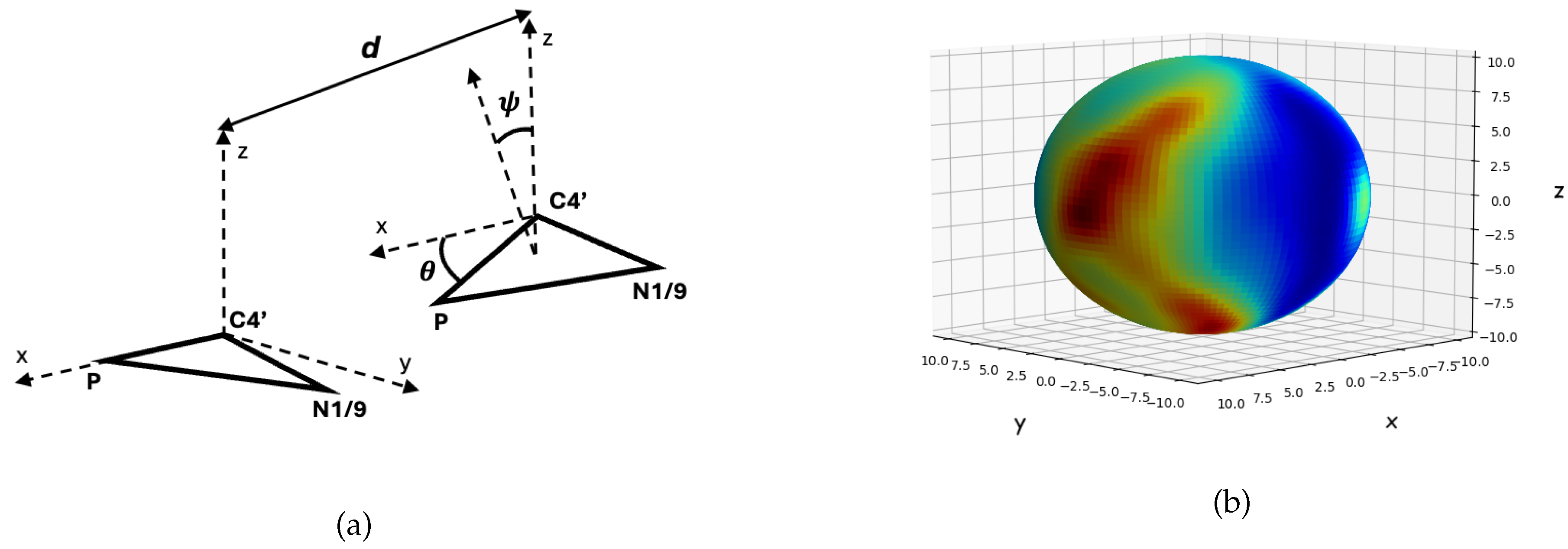
Using the all RNA structures available in the dataset, all nucleotide pairs having tertiary-structure edge types between them were identified. Euclidean distance and relative orientation between each of the corresponding node pairs were considered for further analysis. Value d was a scalar representing Euclidean distance between the C4’ coordinates of the two nucleotides. Filtering for Euclidean distance of in Åresulted in around 43 thousand such pairs. As illustrated in Figure A1(a), the relative orientation was defined in terms of spherical coordinates with being the angle from the positive z-axis and being the angle between the radial line and a polar axis. Angle was defined as the angle between normal vectors of the two (C4’,P,N1/9) planes of the two nucleotides. Angle was defined as the angle between the two C4’-P vectors. The density plot of the normalized relative orientation of the nucleotide pairs is shown in Figure A1(b). Red represents high-density and blue represents low-density orientations. Certain relative pairwise orientations were extremely rare in 3D space. In particular, relative orientations with angle were not found, regardless of values of or d. On the other hand, certain orientations such as were more prevalent representing an uneven distribution of relative orientations.
Figure A1.
Relative orientations of distant nucleotide pairs having tertiary-structure edge types. a) Angle was defined as the angle between normal vectors of the two (C4’,P,N1/9) planes of the two nucleotides. Angle was defined as the angle between the two C4’-P vectors. b) Density plot of the normalized relative orientation of around 43 thousand nucleotide pairs, taken from RNA structures of the old Dataset. All pairs had Euclidean distance of in Å. Red represents high-density and blue represents low-density orientations.
References
- Doudna, J.A.; Charpentier, E. The new frontier of genome engineering with CRISPR-Cas9. Science 2014, 346, 1258096. [Google Scholar] [CrossRef]
- Pardi, N.; Hogan, M.J.; Porter, F.W.; Weissman, D. MRNA Vaccines — a New Era in Vaccinology. Nature reviews. Drug discover/Nature reviews. Drug discovery 2018, 17, 261–279. [Google Scholar] [CrossRef] [PubMed]
- Metkar, M.; Pepin, C.S.; Moore, M.J. Tailor made: the art of therapeutic mRNA design. Nat. Rev. Drug Discov. 2024, 23, 67–83. [Google Scholar] [CrossRef]
- Bronstein, M.M.; Bruna, J.; Cohen, T.; Veličković, P. Geometric Deep Learning: Grids, Groups, Graphs, Geodesics, and Gauges, 2021, [arXiv:cs.LG/2104.13478].
- Jumper, J.; Evans, R.; Pritzel, A.; Green, T.; Figurnov, M.; Ronneberger, O.; Tunyasuvunakool, K.; Bates, R.; Žídek, A.; Potapenko, A.; et al. Highly accurate protein structure prediction with AlphaFold. Nature 2021, 596, 583–589. [Google Scholar] [CrossRef]
- Dauparas, J.; Anishchenko, I.; Bennett, N.; Bai, H.; Ragotte, R.J.; Milles, L.F.; Wicky, B.I.M.; Courbet, A.; de Haas, R.J.; Bethel, N.; et al. Robust deep learning-based protein sequence design using ProteinMPNN. Science 2022, 378, 49–56. [Google Scholar] [CrossRef] [PubMed]
- Watson, J.L.; Juergens, D.; Bennett, N.R.; Trippe, B.L.; Yim, J.; Eisenach, H.E.; Ahern, W.; Borst, A.J.; Ragotte, R.J.; Milles, L.F.; et al. De novo design of protein structure and function with RFdiffusion. Nature 2023, 620, 1089–1100. [Google Scholar] [CrossRef] [PubMed]
- Duval, A.; Mathis, S.V.; Joshi, C.K.; Schmidt, V.; Miret, S.; Malliaros, F.D.; Cohen, T.; Liò, P.; Bengio, Y.; Bronstein, M. A Hitchhiker’s Guide to Geometric GNNs for 3D Atomic Systems, 2024, [arXiv:cs.LG/2312.07511].
- Mandal, M.; Breaker, R.R. Gene regulation by riboswitches. Nat. Rev. Mol. Cell Biol. 2004, 5, 451–463. [Google Scholar] [CrossRef]
- Leppek, K.; Das, R.; Barna, M. Functional 5’ UTR mRNA structures in eukaryotic translation regulation and how to find them. Nat. Rev. Mol. Cell Biol. 2018, 19, 158–174. [Google Scholar] [CrossRef] [PubMed]
- White, H.B.I. Coenzymes as fossils of an earlier metabolic state. Journal of Molecular Evolution 1976, 7, 101–104. [Google Scholar] [CrossRef] [PubMed]
- Benner, S.A.; Ellington, A.D.; Tauer, A. Modern metabolism as a palimpsest of the RNA world. Proceedings of the National Academy of Sciences of the United States of America 1989, 86, 7054–7058. [Google Scholar] [CrossRef] [PubMed]
- Nahvi, A.; Sudarsan, N.; Ebert, M.S.; Zou, X.; Brown, K.L.; Breaker, R.R. Genetic control by a metabolite binding mRNA. Chem. Biol. 2002, 9, 1043. [Google Scholar] [CrossRef] [PubMed]
- Vitreschak, A.G.; Rodionov, D.A.; Mironov, A.A.; Gelfand, M.S. Riboswitches: the oldest mechanism for the regulation of gene expression? Trends Genet. 2004, 20, 44–50. [Google Scholar] [CrossRef] [PubMed]
- Breaker, R.R. Riboswitches: from ancient gene-control systems to modern drug targets. Future Microbiol. 2009, 4, 771–773. [Google Scholar] [CrossRef]
- Breaker, R.R. Riboswitches and the RNA world. Cold Spring Harb. Perspect. Biol. 2012, 4, a003566–a003566. [Google Scholar] [CrossRef] [PubMed]
- Sherwood, A.V.; Henkin, T.M. Riboswitch-mediated gene regulation: Novel RNA architectures dictate gene expression responses. Annu. Rev. Microbiol. 2016, 70, 361–374. [Google Scholar] [CrossRef] [PubMed]
- McCown, P.J.; Corbino, K.A.; Stav, S.; Sherlock, M.E.; Breaker, R.R. Riboswitch diversity and distribution. RNA 2017, 23, 995–1011. [Google Scholar] [CrossRef]
- Breaker, R.R. Riboswitches and translation control. Cold Spring Harb. Perspect. Biol. 2018, 10, a032797. [Google Scholar] [CrossRef]
- Roth, A.; Breaker, R.R. The structural and functional diversity of metabolite-binding riboswitches. Annu. Rev. Biochem. 2009, 78, 305–334. [Google Scholar] [CrossRef]
- Serganov, A.; Nudler, E. A Decade of Riboswitches. Cell 2013, 152, 17–24. [Google Scholar] [CrossRef]
- Peselis, A.; Serganov, A. Themes and variations in riboswitch structure and function. Biochim. Biophys. Acta 2014, 1839, 908–918. [Google Scholar] [CrossRef]
- Breaker, R.R. The biochemical landscape of riboswitch ligands. Biochemistry 2022, 61, 137–149. [Google Scholar] [CrossRef] [PubMed]
- Blount, K.F.; Breaker, R.R. Riboswitches as antibacterial drug targets. Nat. Biotechnol. 2006, 24, 1558–1564. [Google Scholar] [CrossRef] [PubMed]
- Deigan, K.E.; Ferré-D’Amaré, A.R. Riboswitches: discovery of drugs that target bacterial gene-regulatory RNAs. Acc. Chem. Res. 2011, 44, 1329–1338. [Google Scholar] [CrossRef] [PubMed]
- Mehdizadeh Aghdam, E.; Hejazi, M.S.; Barzegar, A. Riboswitches: From living biosensors to novel targets of antibiotics. Gene 2016, 592, 244–259. [Google Scholar] [CrossRef] [PubMed]
- Panchal, V.; Brenk, R. Riboswitches as drug targets for antibiotics. Antibiotics (Basel) 2021, 10, 45. [Google Scholar] [CrossRef] [PubMed]
- Suess, B.; Weigand, J.E. Engineered riboswitches: overview, problems and trends. RNA Biol. 2008, 5, 24–29. [Google Scholar] [CrossRef]
- Link, K.H.; Breaker, R.R. Engineering ligand-responsive gene-control elements: lessons learned from natural riboswitches. Gene Ther. 2009, 16, 1189–1201. [Google Scholar] [CrossRef] [PubMed]
- Schmidt, C.M.; Smolke, C.D. RNA switches for synthetic biology. Cold Spring Harb. Perspect. Biol. 2019, 11, a032532. [Google Scholar] [CrossRef]
- Wickiser, J.K.; Winkler, W.C.; Breaker, R.R.; Crothers, D.M. The speed of RNA transcription and metabolite binding kinetics operate an FMN riboswitch. Mol. Cell 2005, 18, 49–60. [Google Scholar] [CrossRef] [PubMed]
- Ariza-Mateos, A.; Nuthanakanti, A.; Serganov, A. Riboswitch mechanisms: New tricks for an old dog. Biochemistry (Mosc.) 2021, 86, 962–975. [Google Scholar] [CrossRef]
- Kavita, K.; Breaker, R.R. Discovering riboswitches: the past and the future. Trends Biochem. Sci. 2023, 48, 119–141. [Google Scholar] [CrossRef]
- Churkin, A.; Retwitzer, M.D.; Reinharz, V.; Ponty, Y.; Waldispühl, J.; Barash, D. Design of RNAs: comparing programs for inverse RNA folding. Brief. Bioinform. 2018, 19, 350–358. [Google Scholar] [CrossRef]
- Runge, F.; Franke, J.; Fertmann, D.; Backofen, R.; Hutter, F. Partial RNA design. Bioinformatics 2024, 40, i437–i445. [Google Scholar] [CrossRef] [PubMed]
- Lorenz, R.; Bernhart, S.H.; Höner zu Siederdissen, C.; Tafer, H.; Flamm, C.; Stadler, P.F.; Hofacker, I.L. ViennaRNA Package 2.0. Algorithms for Molecular Biology 2011, 6, 26. [Google Scholar] [CrossRef]
- Leman, J.K.; Weitzner, B.D.; Lewis, S.M.; Adolf-Bryfogle, J.; Alam, N.; Alford, R.F.; Aprahamian, M.; Baker, D.; Barlow, K.A.; Barth, P.; et al. Macromolecular modeling and design in Rosetta: recent methods and frameworks. Nat. Methods 2020, 17, 665–680. [Google Scholar] [CrossRef]
- Tan, C.; Zhang, Y.; Gao, Z.; Hu, B.; Li, S.; Liu, Z.; Li, S.Z. RDesign: Hierarchical Data-efficient Representation Learning for Tertiary Structure-based RNA Design. In Proceedings of the The Twelfth International Conference on Learning Representations; 2024. [Google Scholar]
- Huang, H.; Lin, Z.; He, D.; Hong, L.; Li, Y. RiboDiffusion: tertiary structure-based RNA inverse folding with generative diffusion models. Bioinformatics 2024, 40, i347–i356. [Google Scholar] [CrossRef] [PubMed]
- Joshi, C.K.; Jamasb, A.R.; Viñas, R.; Harris, C.; Mathis, S.; Liò, P. Multi-State RNA Design with Geometric Multi-Graph Neural Networks. arXiv preprint 2023. [Google Scholar]
- Jing, B.; Eismann, S.; Suriana, P.; Townshend, R.J.L.; Dror, R.O. Learning from Protein Structure with Geometric Vector Perceptrons. ArXiv 2020, abs/2009.01411.
- Das, R.; Karanicolas, J.; Baker, D. Atomic accuracy in predicting and designing noncanonical RNA structure. Nat. Methods 2010, 7, 291–294. [Google Scholar] [CrossRef]
- oshi, C.K.; Jamasb, A.R.; Viñas, R.; Harris, C.; Mathis, S.V.; Morehead, A.; Anand, R.; Liò, P. gRNAde: Geometric Deep Learning for 3D RNA inverse design. bioRxiv 2024, [https://www.biorxiv.org/content/early/2024/05/25/2024.03.31.587283.full.pdf]. [CrossRef]
- Lu, X.; Olson, W.K. 3DNA: a software package for the analysis, rebuilding and visualization of three‚Äêdimensional nucleic acid structures. Nucleic Acids Research 2003, 31, 5108–5121. [Google Scholar] [CrossRef]
- Lu, X.J.; Bussemaker, H.J.; Olson, W.K. DSSR: an integrated software tool for dissecting the spatial structure of RNA. Nucleic Acids Research 2015, 43, e142–e142. [Google Scholar] [CrossRef] [PubMed]
- Fey, M.; Lenssen, J.E. Fast graph representation learning with PyTorch Geometric 2019.
- Schrödinger, LLC. The PyMOL Molecular Graphics System, Version 1.8, 2015.
- Adamczyk, B.; Antczak, M.; Szachniuk, M. RNAsolo: a repository of cleaned PDB-derived RNA 3D structures. Bioinformatics 2022, 38, 3668–3670. [Google Scholar] [CrossRef] [PubMed]
- Fu, L.; Niu, B.; Zhu, Z.; Wu, S.; Li, W. CD-HIT: accelerated for clustering the next-generation sequencing data. Bioinformatics 2012, 28, 3150–3152. [Google Scholar] [CrossRef] [PubMed]
- Zhang, C.; Shine, M.; Pyle, A.M.; Zhang, Y. US-align: universal structure alignments of proteins, nucleic acids, and macromolecular complexes. Nat. Methods 2022, 19, 1109–1115. [Google Scholar] [CrossRef] [PubMed]
- Wayment-Steele, H.K.; Kladwang, W.; Strom, A.I.; Lee, J.; Treuille, A.; Becka, A.; Eterna Participants. ; Das, R. RNA secondary structure packages evaluated and improved by high-throughput experiments. Nat. Methods 2022, 19, 1234–1242. [Google Scholar] [CrossRef] [PubMed]
- Dawson, W.K.; Maciejczyk, M.; Jankowska, E.J.; Bujnicki, J.M. Coarse-grained modeling of RNA 3D structure. Methods 2016, 103, 138–156. [Google Scholar] [CrossRef]
- Leontis, N.B.; Westhof, E. Geometric nomenclature and classification of RNA base pairs. RNA 2001, 7, 499–512. [Google Scholar] [CrossRef] [PubMed]
- Ingraham, J.; Garg, V.; Barzilay, R.; Jaakkola, T. Generative Models for Graph-Based Protein Design. In Proceedings of the Advances in Neural Information Processing Systems; Wallach, H.; Larochelle, H.; Beygelzimer, A.; d’Alché-Buc, F.; Fox, E.; Garnett, R., Eds. Curran Associates, Inc., Vol. 32. 2019. [Google Scholar]
- Williams, R.J.; Zipser, D. A Learning Algorithm for Continually Running Fully Recurrent Neural Networks. Neural Computation 1989, 1, 270–280. [Google Scholar] [CrossRef]
- Sarver, M.; Zirbel, C.L.; Stombaugh, J.; Mokdad, A.; Leontis, N.B. FR3D: finding local and composite recurrent structural motifs in RNA 3D structures. J. Math. Biol. 2008, 56, 215–252. [Google Scholar] [CrossRef] [PubMed]
- Lee, H.K.; Lee, Y.T.; Fan, L.; Wilt, H.M.; Conrad, C.E.; Yu, P.; Zhang, J.; Shi, G.; Ji, X.; Wang, Y.X.; et al. Crystal structure of <em>Escherichia coli</em> thiamine pyrophosphate-sensing riboswitch in the apo state. Structure 2023, 31, 848–859.e3. [Google Scholar] [CrossRef]
- Abramson, J.; Adler, J.; Dunger, J.; Evans, R.; Green, T.; Pritzel, A.; Ronneberger, O.; Willmore, L.; Ballard, A.J.; Bambrick, J.; et al. Accurate structure prediction of biomolecular interactions with AlphaFold 3. Nature 2024, 630, 493–500. [Google Scholar] [CrossRef]
- Oliver, C.; Mallet, V.; Waldisp√ºhl, J. , A.; Barash, D., Eds.; Springer US: New York, NY, 2025; pp. 153–161. https://doi.org/10.1007/978-1-0716-4079-1_10.rnaglib. In RNA Design: Methods and Protocols; Churkin, A., Barash, D., Eds.; Springer US: New York, NY, 2025; Springer US: New York, NY, 2025; pp. 153–161. [Google Scholar] [CrossRef]
- Al-Fatlawi, A.; Hossen, M.B.; El-Hendi, F.; Schroeder, M. Protein secondary structure and remote homology detection. bioRxiv 2024, [https://www.biorxiv.org/content/early/2024/09/06/2024.09.03.611022.full.pdf]. [CrossRef]
| 1 | Lower perplexity does not always reflect a more superior model. It may be possible to have slightly high perplexity/entropy for individual nucleotide probabilities but a low perplexity/entropy on their joint distributions. |
Figure 1.
The three different edge types of the RNA structure graph. a) Structure corresponds to part of the immature 30S ribosomal subunit from Staphylococcus aureus, 8BH7|1|a. Nucleotides having different edge types are shown in blue (for secondary-structure edge types) and magenta (for tertiary-structure edge types). One of the tertiary-structure edges occurs between C169 and A1457 with length 11.9Å, PDB coordinates. Figure drawn using PyMOL [47]. b) Corresponding primary-structure edge types are shown in orange. Secondary-structure edge types for three base pairs (six nucleotides) are shown in blue. Tertiary-structure edge types for two edges are shown in magenta.
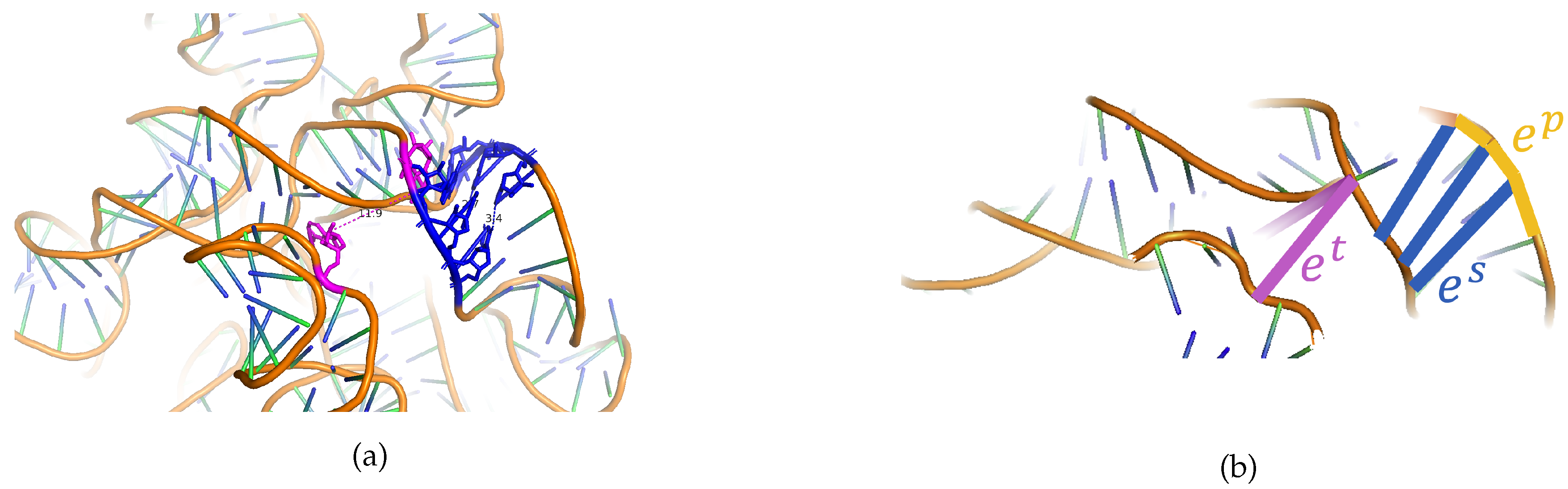
Figure 2.
Data statistics. PDB files were downloaded from the RNAsolo web server [48] on August 1, 2024. (a) Histogram of sequence lengths. (b) Histogram of number of structures per unique sequence.
Figure 2.
Data statistics. PDB files were downloaded from the RNAsolo web server [48] on August 1, 2024. (a) Histogram of sequence lengths. (b) Histogram of number of structures per unique sequence.
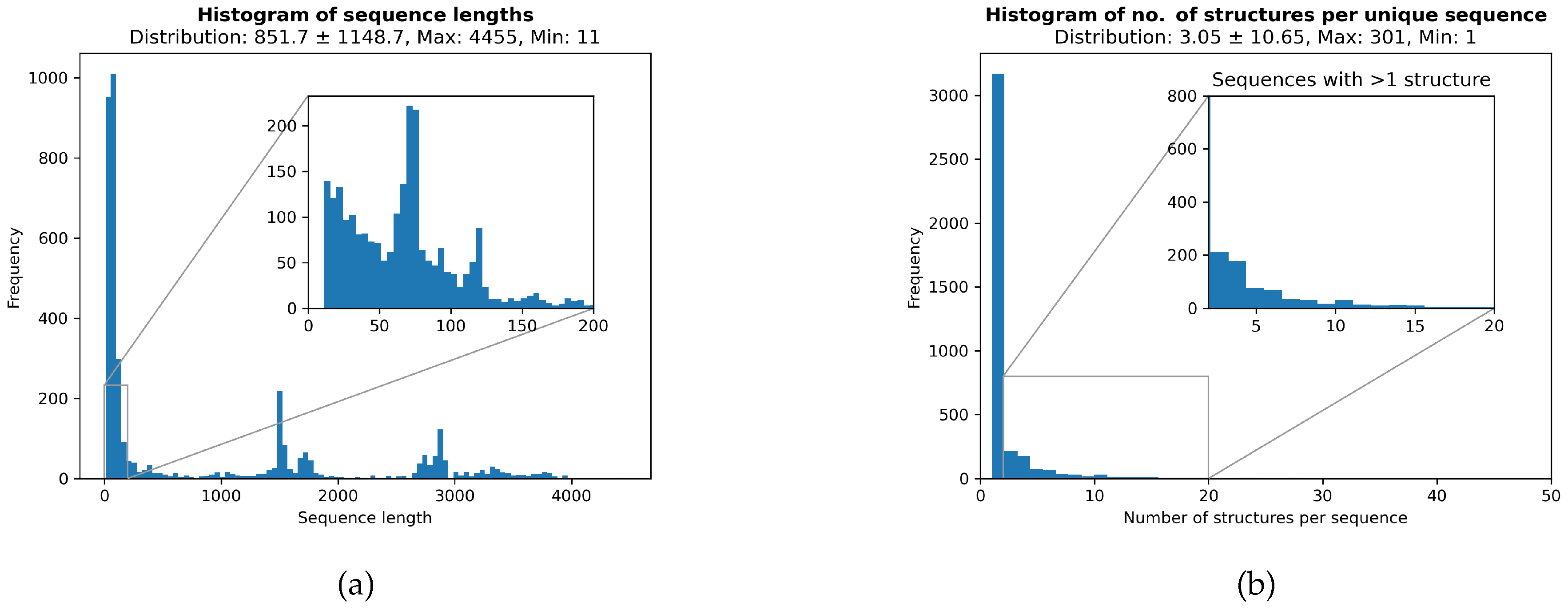
Figure 3.
Number of primary-, secondary-, and tertiary-structure edge types with respect to sequence length. Light magenta represents the original count of tertiary-structure edges. The magenta dashed line shows the cut-off value tertiary-structure edge number. Edges of RNAs with higher counts were down-sampled to have strictly matched the threshold
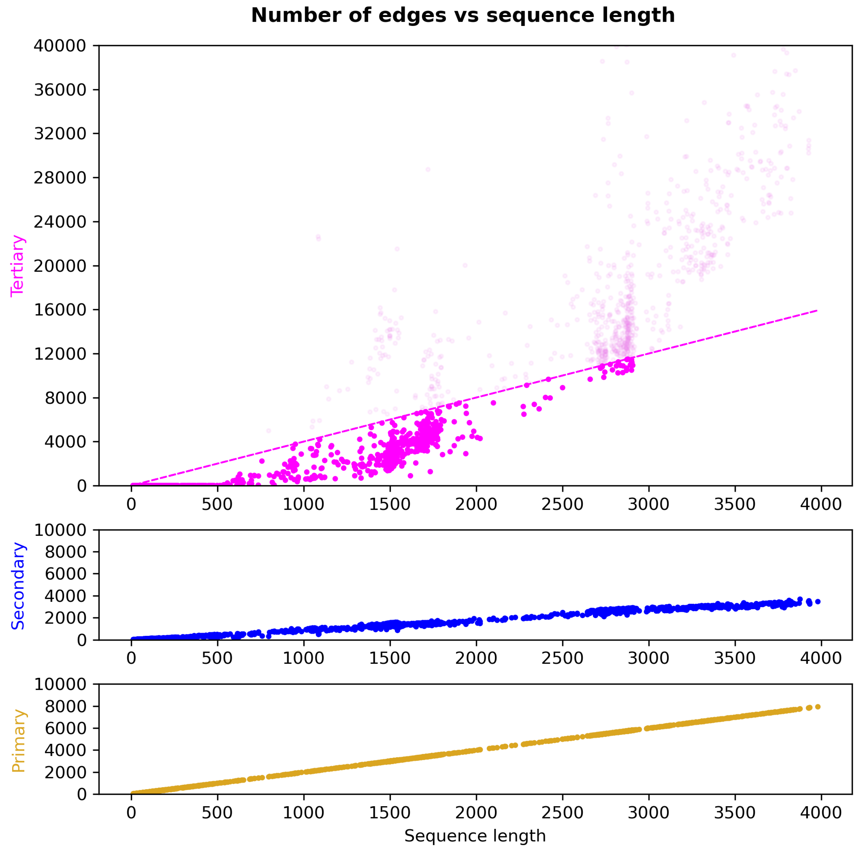
Figure 4.
Secondary-structure-informed relational graph neural network diagram for the NAR-informed model. Node and edge embeddings of each structure k are fed into L cascaded layers of relational GNNs. Each layer is composed of three GVP-GNNs acting on their own primary-, secondary-, and tertiary-structure edge types, shown in orange, blue, and magenta, respectively. Messages are pooled to produce a single message used to update node embedding before feeding it into the next layer. Final updated node embeddings corresponding to individual structures are then pooled to produce final nucleotide probabilities using a linear model in the decoder
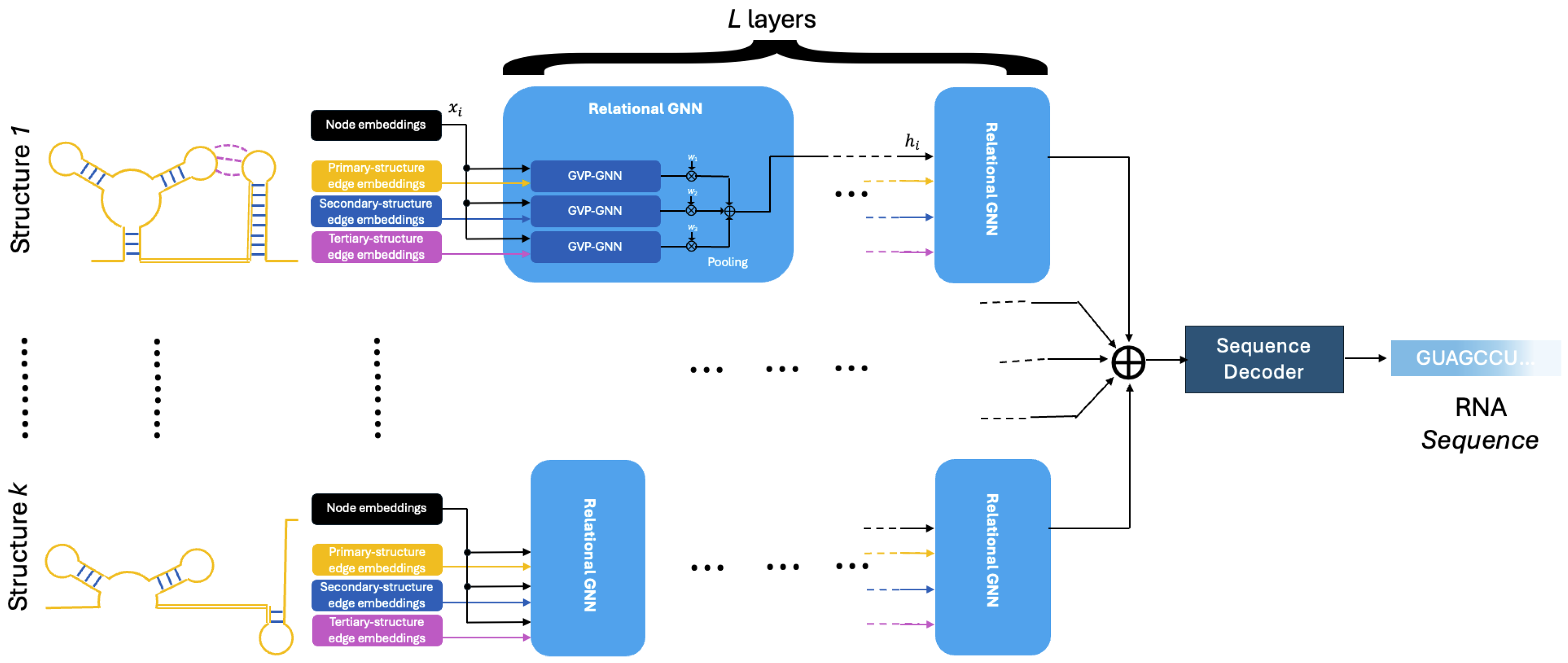
Figure 5.
The apo structure of the TPP riboswitch aptamer PDB ID 8F4O along with the predicted structure of its corresponding designed sequence using seqid-trained AR-informed-3D. True and predicted structures are shown in orange and green, respectively. The first and last nucleotides of both structures are shown in licorice mode for ease of visualization. Aligned structures had RMSD of (15.88Å) among all their atoms and RMSD of (16.38Å) among their C4’ atoms. Predicted structure obtained via AlphaFold 3 [58]. The disconnects in the true structure are due to numbering schemes in the corresponding PDB file.
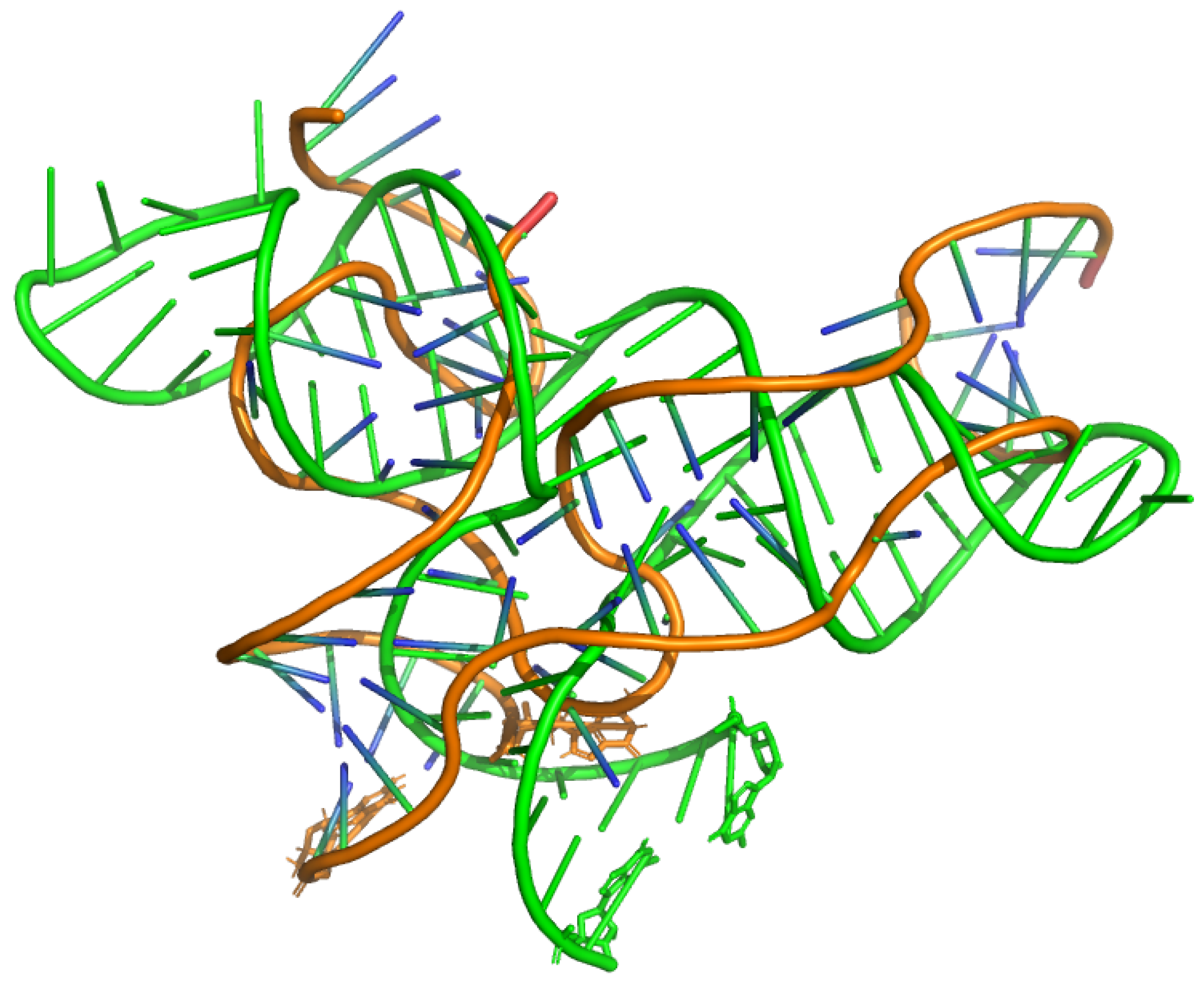

Table 1.
Model performance comparison between the original gRNAde and the secondary-structure-informed relational graph neural network. Performance corresponds to 100 epochs. Mean Recovery is expected to have standard deviation [40]. Abbreviations: Ppl. = Perplexity, Acc. = Accuracy, Rec. = Recovery, SC = SC score.
| model | split | layers | Ppl. (↓) | Acc. (↑) | Rec. (↑) | SC (↑) |
|---|---|---|---|---|---|---|
| AR-original | seqid | 4 | 1.2501 | 66.08 | 50.84 | 63.18 |
| AR-informed-2D | seqid | 2 | 1.4875 | 71.12 | 54.51 | 53.00 |
| AR-informed-3D | seqid | 2 | 1.4136 | 71.84 | 54.10 | 52.32 |
| AR-informed-3D | seqid | 4 | 1.3526 | 72.24 | 58.37 | 52.92 |
| AR-original | structsim | 4 | 1.4843 | 62.72 | 44.85 | 55.41 |
| AR-informed-2D | structsim | 2 | 1.3422 | 68.61 | 50.31 | 51.06 |
| AR-informed-3D | structsim | 2 | 1.3471 | 68.66 | 49.40 | 51.59 |
| AR-informed-3D | structsim | 4 | 1.2984 | 69.02 | 50.23 | 54.57 |
| NAR-original | seqid | 4 | 1.5790 | 53.95 | 53.62 | 38.68 |
| NAR-informed-2D | seqid | 2 | 1.6062 | 59.87 | 61.06 | 42.44 |
| NAR-informed-3D | seqid | 2 | 1.4562 | 60.17 | 61.92 | 30.66 |
| NAR-informed-3D | seqid | 4 | 1.5483 | 61.02 | 61.39 | 0.4840 |
| NAR-original | structsim | 4 | 1.9695 | 47.18 | 43.51 | 39.36 |
| NAR-informed-2D | structsim | 2 | 1.4444 | 56.25 | 55.07 | 25.22 |
| NAR-informed-3D | structsim | 2 | 1.4398 | 54.97 | 51.44 | 26.37 |
| NAR-informed-3D | structsim | 4 | 1.3413 | 56.59 | 53.00 | 40.83 |
Table 2.
Performance comparison for the 14 structures of interest ([42], Supplementary Table 2). AR-informed refers to the seqid-trained AR-informed-3D with four layers. Recovery values for AR-informed were computed over 16 sampled sequences for each structure. All other Recovery values are according to [43]. Abbreviations: VRNA = ViennaRNA, RDes. = RDesign, Ros. = Rosetta, and AR-3D = seqid-trained AR-informed-3D.
| PDB | Desc. | VRNA | RDes. | Ros. | gRNAde | AR-3D |
|---|---|---|---|---|---|---|
| 1CSL | RRE high affinity site | 0.25 | 0.4455 | 0.44 | 0.5719 | 0.4263 |
| 1ET4 | RNA aptamer | 0.25 | 0.3929 | 0.44 | 0.6250 | 0.4379 |
| 1F27 | RNA pseudoknot | 0.30 | 0.3013 | 0.37 | 0.3437 | 0.3750 |
| 1L2X | RNA pseudoknot | 0.24 | 0.3727 | 0.48 | 0.4721 | 0.5765 |
| 1LNT | internal loop of SRP | 0.33 | 0.5556 | 0.53 | 0.5843 | 0.7131 |
| 1Q9A | Sarcin/ricin dom. | 0.27 | 0.4417 | 0.41 | 0.5044 | 0.8079 |
| 4FE5 | Guanine riboswitch | 0.29 | 0.4112 | 0.36 | 0.5300 | 0.7687 |
| 1X9C | All-RNA hairpin ribozyme | 0.26 | 0.3967 | 0.50 | 0.5000 | 0.3927 |
| 1XPE | HIV-1 B RNA | 0.27 | 0.3834 | 0.40 | 0.7037 | 0.4266 |
| 2GCS | glmS ribozyme | 0.25 | 0.4518 | 0.44 | 0.5078 | 0.6659 |
| 2GDI | TPP riboswitch | 0.25 | 0.3523 | 0.48 | 0.6500 | 0.7680 |
| 2OEU | Junctionless hairpin riboz. | 0.23 | 0.5000 | 0.37 | 0.9519 | 0.7680 |
| 2R8S | Tetrahymena ribozyme | 0.27 | 0.5641 | 0.53 | 0.5689 | 0.6985 |
| 354D | Loop E | 0.28 | 0.4458 | 0.55 | 0.4410 | 0.8210 |
| Overall recovery: | 0.27 | 0.4296 | 0.45 | 0.5682 | 0.6044 |
Table 3.
True and predicted sequence for the apo structure of the TPP riboswitch aptamer. The sequence 8F4O_1_B was 65nt. The predicted sequence, Pred_1, was obtained from passing the experimentally-derived structure of 8F4O to the seqid-trained AR-informed-3D model. Pred_1 recovery was 0.7692.
Table 3.
True and predicted sequence for the apo structure of the TPP riboswitch aptamer. The sequence 8F4O_1_B was 65nt. The predicted sequence, Pred_1, was obtained from passing the experimentally-derived structure of 8F4O to the seqid-trained AR-informed-3D model. Pred_1 recovery was 0.7692.
| name | sequence |
|---|---|
| 8F4O_1_B | GCGACUCGGGGUGAAGGCUGAGAAAUACCCGUAUCACCUGAUCUGGAGCCAGCGUAGGGAAGUCG |
| Pred_1 | GCGCCUCGGGGUGAAAGCUGAGAAAUACCGGUAGCACUUCUUUUCGUUCGAACGUAAGGAAGGCG |
Disclaimer/Publisher’s Note: The statements, opinions and data contained in all publications are solely those of the individual author(s) and contributor(s) and not of MDPI and/or the editor(s). MDPI and/or the editor(s) disclaim responsibility for any injury to people or property resulting from any ideas, methods, instructions or products referred to in the content. |
© 2024 by the authors. Licensee MDPI, Basel, Switzerland. This article is an open access article distributed under the terms and conditions of the Creative Commons Attribution (CC BY) license (http://creativecommons.org/licenses/by/4.0/).
Copyright: This open access article is published under a Creative Commons CC BY 4.0 license, which permit the free download, distribution, and reuse, provided that the author and preprint are cited in any reuse.


