
Submitted:
24 December 2024
Posted:
25 December 2024
You are already at the latest version
Abstract
In the field of ensemble learning, bagging and stacking are two widely used ensemble strategies. Bagging enhances model robustness through repeated sampling and weighted averaging of homogeneous classifiers, while stacking improves classification performance by integrating multiple models using meta-learning strategies, taking advantage of the diversity of heterogeneous classifiers. However, the fixed weight distribution strategy in traditional bagging methods often has limitations when handling complex or imbalanced datasets. This paper combines the concept of heterogeneous classifier integration in stacking with the weighted averaging strategy of bagging, proposing a new adaptive weight distribution approach to enhance bagging's performance in heterogeneous ensemble settings. Specifically, we propose three weight generation functions with "high at both ends, low in the middle" curve shapes, and demonstrate the superiority of this strategy over fixed weight methods on two datasets. Additionally, we design a specialized neural network, and by training it adequately, validate the rationality of the proposed adaptive weight distribution strategy, further improving the model's robustness. Experimental results show that this method is particularly effective in scenarios with class imbalance and is applicable to classification tasks with imbalanced classes, such as anomaly detection.
Keywords:
ensemble learning
; bagging
; stacking
; adaptive weight generation
; anomaly detection
1. Introduction
1.1. Background
A classifier is a system that takes instances from a dataset and assigns a category or label to each instance. To accomplish this task, a classifier needs to possess certain knowledge. Classifiers can be created through various learning methods, such as deduction, analogy, or memorization, but the most common approach is to learn knowledge from a set of pre-classified instances, a method known as supervised learning. Much of machine learning research focuses on developing automated approaches for classification tasks. Despite the proposal of various models, such as artificial neural networks, decision trees, inductive logic programming, and Bayesian learning algorithms, building a perfect classifier for any specific task remains a challenging endeavor. Furthermore, no single method can be considered superior across all datasets. As a result, combining different classification models has become a viable choice for achieving higher accuracy, known as ensemble learning. The core idea of ensemble learning is to create a set of classifiers and combine their outputs such that the ensemble’s performance surpasses that of any individual classifier. To achieve this, it is necessary to ensure that (1) each classifier is both accurate and diverse, and (2) the combination of outputs amplifies correct decisions and mitigates erroneous ones. Research in ensemble learning often focuses on generating multiple classifiers using a single learning algorithm and combining their outputs using mathematical functions. Stacking, on the other hand, generates classifier members through various learning algorithms and subsequently uses another algorithm to learn how to combine their outputs [1].
Currently, commonly used ensemble methods include Boosting, Bagging, and Stacking, each with its unique strategies and applicable scenarios. Boosting is an iterative ensemble method aimed at reducing the bias between the base classifier’s output and the true labels, gradually bringing the output closer to the true labels. Typical Boosting methods, such as AdaBoost and Gradient Boosting, have demonstrated excellent performance in various classification and regression tasks. Bagging is an ensemble method that generates homogeneous classifiers through repeated sampling and parallel training, reducing the model’s variance and enhancing robustness. A representative algorithm of Bagging is Random Forest, which trains multiple decision trees on different subsets and makes predictions through averaging or voting, effectively reducing overfitting risks. Stacking, another ensemble method, focuses on improving performance through the combination of heterogeneous classifiers. It generates various base classifiers in the first layer and uses a meta-learner in the second layer to learn how to combine their outputs for better prediction accuracy [2].
This paper focuses on Bagging and Stacking. While both Bagging and Stacking have important applications in ensemble learning, they each have notable limitations. In Bagging, the traditional fixed-weight combination strategy often fails to achieve satisfactory results when dealing with class imbalance problems. Although Stacking can integrate heterogeneous classifiers, it lacks a directly effective and interpretable weighting strategy for combining their outputs. To address these limitations, this paper proposes a novel approach that combines the heterogeneous classifier integration idea of Stacking with the weighted averaging strategy of Bagging, using an adaptive weight distribution strategy to improve the performance of Bagging. We design three weight generation functions with “high at both ends, low in the middle” curve shapes and experimentally demonstrate the advantages of this strategy in heterogeneous classifier integration. Additionally, we construct a specialized neural network and loss function to further validate the rationale behind the weight distribution strategy, achieving excellent performance on imbalanced datasets. The innovation of this paper lies in the introduction of an adaptive weighting strategy for heterogeneous classifier integration, overcoming the limitations of traditional Bagging and Stacking, and showing significant advantages, particularly in class-imbalanced tasks.
1.2. Related Work
Junlang Wang et al. proposed a method for multi-component fault diagnosis in hydraulic systems. The method first uses Pearson correlation coefficients and Neighborhood Component Analysis (NCA) for data channel selection and feature dimensionality reduction, to reduce data redundancy and improve computational efficiency. Two different types of Deep Neural Networks (DNNs) are then constructed as base learners: Stacked Sparse Autoencoder and Deep Hierarchical Extreme Learning Machine (D-ELM). A Bagging voting ensemble strategy is used to combine these DNN base learners to enhance the robustness and accuracy of the diagnostic system. This paper utilizes the original Bagging voting ensemble strategy, where multiple learners vote for a sample, and the class with the most votes is assigned as the predicted class for the sample [3].
Yufei Xia et al. introduced a trainable combiner to optimize the ensemble results, training an XGBoost model as a meta-classifier to learn how to generate the final prediction based on the outputs of base learners. However, this meta-classifier is prediction-oriented and lacks interpretability in terms of the weight distribution of each base learner [4].
V. Sobanadevi and G. Ravi proposed a heterogeneous ensemble-based model (HBSE) for credit card fraud detection, training a logistic regression model as a Level-1 meta-learner, using the outputs of Level-0 base learners as input, and producing the final prediction. Similar to the previous paper, this approach also lacks interpretability in the weight distribution of each base learner [5].
M. Paz Sesmero et al. provided a detailed discussion of various variants of the Stacking method, which was first proposed by Wolpert in 1992 [1]. For instance, Skalak introduced the use of instance-based learning classifiers as Level-0 classifiers (base learners). In this variant, base learners are no longer traditional machine learning models, but instead classify by storing a few prototypes for each class [6]. Fan et al. proposed a method to evaluate the overall accuracy of a Stacking ensemble model using conflict-based accuracy estimates, employing two tree-based classifiers and one rule-based classifier as base learners. For the Level-1 meta-learner, they used a non-pruned decision tree instead of a traditional decision tree [7]. Merz proposed another variant of Stacking, called SCANN (Stacking with Correspondence Analysis and Nearest Neighbor). In this approach, correspondence analysis is used to detect correlations between base learners, effectively removing redundant information. After removing the dependency between base learners, a nearest-neighbor method is used as the meta-learner in the new feature space. SCANN improves model diversity and handles heterogeneous base learners effectively [8]. Ting and Witten proposed several important innovations, including using class probabilities rather than single class predictions as the output of Level-0 classifiers and using Multi-response Linear Regression (MLR) as the Level-1 classifier. While class probabilities were used as inputs to Level-1, the output was still the final prediction, which remained result-oriented and lacked interpretability in the weight distribution of base learners [9].
Hossein Ghaderi Zefrehi et al. addressed the class imbalance problem in classification tasks, proposing a solution using heterogeneous ensembles. In binary classification, class imbalance typically refers to situations where one class has far more samples than the other, leading to poor performance on the minority class. The paper mentions that ensemble classifiers can alleviate this issue by using different sampling methods, especially by applying different balanced datasets to each member of the ensemble, with the datasets generated via random undersampling or oversampling [10].
Qiang Li Zhao et al. explored classifier ensemble methods in incremental learning, proposing a new Bagging-based incremental learning method called Bagging++. In this method, incremental base learners are trained on new data and integrated into the original ensemble model after training. This paper also uses the simple voting ensemble strategy [11].
Kuo-Wei Hsu et al. theoretically demonstrated that the greater the divergence (heterogeneity) between base classifier algorithms in an ensemble, the stronger the resulting model and the more robust its performance. They designed a Bagging framework based on heterogeneous base classifiers, but the final fusion strategy for combining the results of base classifiers was not explored, and the original Bagging voting strategy was still used [12].
Nguyen et al. proposed an ensemble selection method based on classifier prediction confidence, which takes into account both the classifier’s prediction confidence on test samples and its overall reliability. In this method, a classifier’s prediction result is selected only if its confidence exceeds its reliability threshold. By optimizing the empirical 0-1 loss on the training set, this method effectively combines the characteristics of static and dynamic ensemble selection, and experimental results on 62 datasets show that this method outperforms various traditional ensemble strategies [13].
In summary, existing research based on Stacking generally produces final predictions in the meta-classifier of the last layer, with a strong focus on result-oriented output and lacking interpretability in the weight distribution of individual base classifiers. In contrast, Bagging-based research mainly focuses on improving the performance and robustness of the model by introducing heterogeneous base classifiers, but still retains the original Bagging method’s strategy for combining base learner results, which typically involves voting ensemble or fixed-weight averaging. Some ensemble methods based on classifier prediction confidence attempt to find suitable thresholds to determine which base learners can participate in the final decision, but ultimately still use simple voting ensemble or fixed-weight averaging strategies.
Based on the related work above, the contributions of this paper are as follows:
- For the final result fusion strategy of Bagging, we propose an intuitive anomaly detection weight allocation strategy: when merging results, if the predicted score (predict probability, also known as prediction confidence) given by a classifier is closer to 0 or 1, it indicates that the classifier has higher confidence in its judgment, and therefore should be assigned higher weight.
- Based on the above weight allocation strategy, three weight generation functions with a “high at both ends, low in the middle” curve are designed, and better results than fixed weight allocation strategies are obtained on two datasets.
- To explore the relationship between the outputs of base learners and weight allocation, a special neural network and loss function are designed. The network’s input is the output of the base learners, and the output is the weight to be allocated. After sufficient training, the function curve drawn by this network is consistent with the proposed weight allocation strategy, proving the reasonableness of the strategy. Since this neural network is trained in a data-driven manner, it generalizes better compared to the weight generation functions with fixed expressions mentioned earlier.
2. Materials and Methods
2.1. Problem Definition
In supervised binary classification tasks, the dataset typically consists of a collection of labeled data pairs, denoted as , where n is the number of samples, represents the feature vector of the i-th sample with m features, and indicates the label of the current sample.
In ensemble learning, the final result of the ensemble model is usually obtained by combining the outputs of multiple base learners. Let denote the set of well-trained base learners, where J is the number of base learners. Each base learner can be considered as a function, expressed as .
In the result fusion of bagging ensemble methods, two common strategies are voting and averaging. The voting method is expressed as
where represents the weight of the j-th learner, and is the indicator function, which takes the value 1 when , and 0 otherwise.
The weighted averaging method is expressed as
where is the weight of the j-th learner, and . This paper mainly investigates the relationship between and in the weighted averaging method, which can be considered as a function, having the functional form
Thus, we can rewrite Equation (2) as
By extending the range of from to the entire real number domain R, we rewrite Equation (4) as
Nguyen et al. point out in their paper that the higher the classifier’s prediction confidence, the higher its weight in the ensemble should be [13]. Specifically, in anomaly detection or binary classification tasks, when a classifier’s predicted score for a certain class (often the anomaly class) is closer to 0 or 1, it indicates that the classifier has higher confidence in this decision and should therefore be assigned a higher weight. Visualizing this, the function graph of should exhibit a "high at both ends, low in the middle" pattern, with being the axis of symmetry.
2.2. Three "High at Both Ends, Low in the Middle" Functions
Based on the problem definition and analysis, three functions that satisfy the "high at both ends, low in the middle" property and are symmetric around are proposed. The first function is the tangent function, transformed by shifting and taking the absolute value (referred to as the tan function hereafter). Its functional expression is:
The graph of this function is shown in Figure 1.
The second function is the secant function, shifted (referred to as the sec function hereafter). Its functional expression is:
The graph of this function is shown in Figure 2.
The third function is a shifted rational function (referred to as the fractional function hereafter). Its functional expression is:
The graph of this function is shown in Figure 3.
As shown, all three functions assign higher weights to base learners whose predicted scores are closer to 0 or 1, while those with predicted scores closer to 0.5 are given smaller weights. Compared to the other two functions, the tan function has a weight of 0 at and carries a risk of division by zero. However, on the domain , the derivative of this function is relatively large at every point, which leads to more pronounced differentiation of the outputs from different base learners. The sec function and the fractional function, on the other hand, have derivatives approaching 0 on the interval , resulting in a smaller and more consistent weight for base learners whose predicted scores fall within this range. For , the derivatives approach infinity, giving base learners in these regions a larger and more distinct weight.
Each of the three functions has its advantages and disadvantages, but none of them are universally applicable to all datasets. Therefore, in the next section, a neural network-based weight generation function is proposed. By cleverly constructing the neural network and designing an appropriate loss function, this function can learn, in a data-driven manner, a weight generation function that is suitable for a specific dataset.
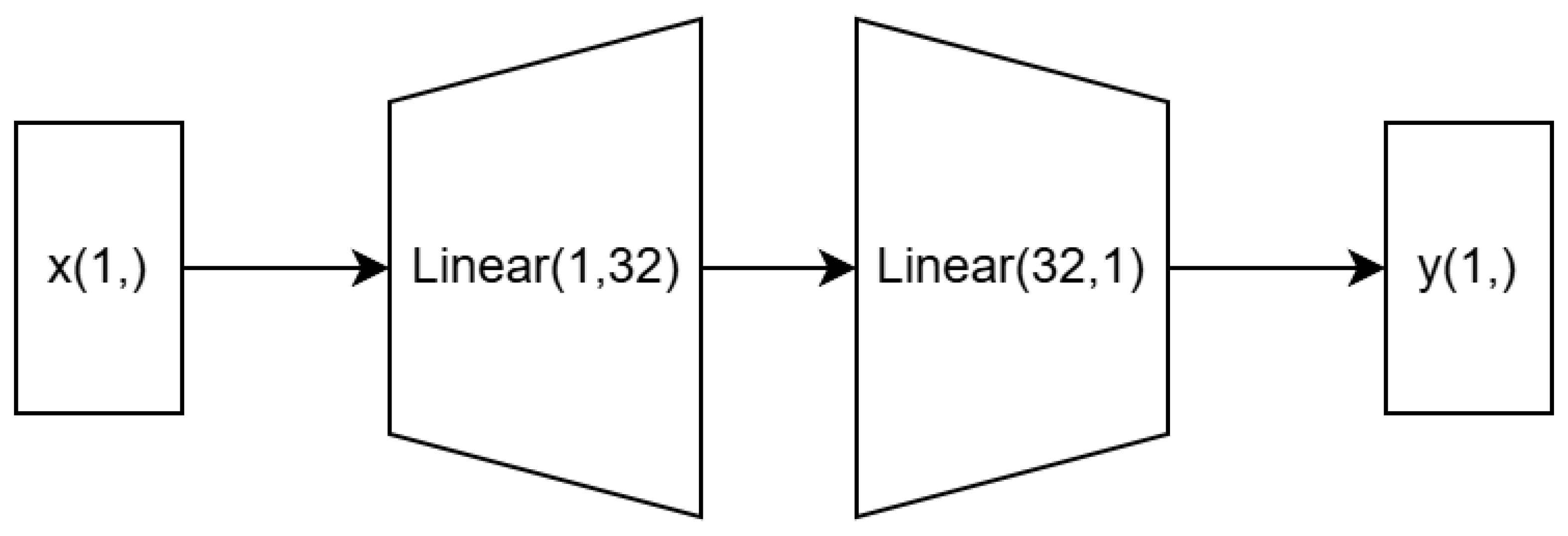
2.3. Neural Network-Based Weight Generation Function
A neural network-based weight generation function is designed, and its overall structure is shown in Figure 4. The outputs of classifiers 1 to J do not interact directly and remain independent until the calculation of the loss function, which is indicated by the dashed lines. The feed-forward neural network (FFN) in the middle receives a scalar as input and outputs a scalar, which represents the weight assigned to the corresponding classifier. The function expression for this part is given in formula (3).
Then, multiple multiplicative skip connections [14] are used to multiply the outputs of each classifier by the assigned weights. The sum of these weighted outputs gives , as shown in formula (5). Finally, the deviation between and the true label y is computed as the loss function. In this case, the mean squared error (MSE) is used as a measure of the deviation between and the true label y, and the loss function is expressed in formula (9).
From formula (5), we can see that the outputs of the classifiers interact within the loss function, and through the backpropagation algorithm, they collectively influence the weights of the neurons in the FFN [15], as shown in formula (10), where denotes the weight of the neuron. This neural network is trained in a data-driven manner and can flexibly adapt to different datasets and combinations of classifiers.
2.4. Datasets and Evaluation Metrics
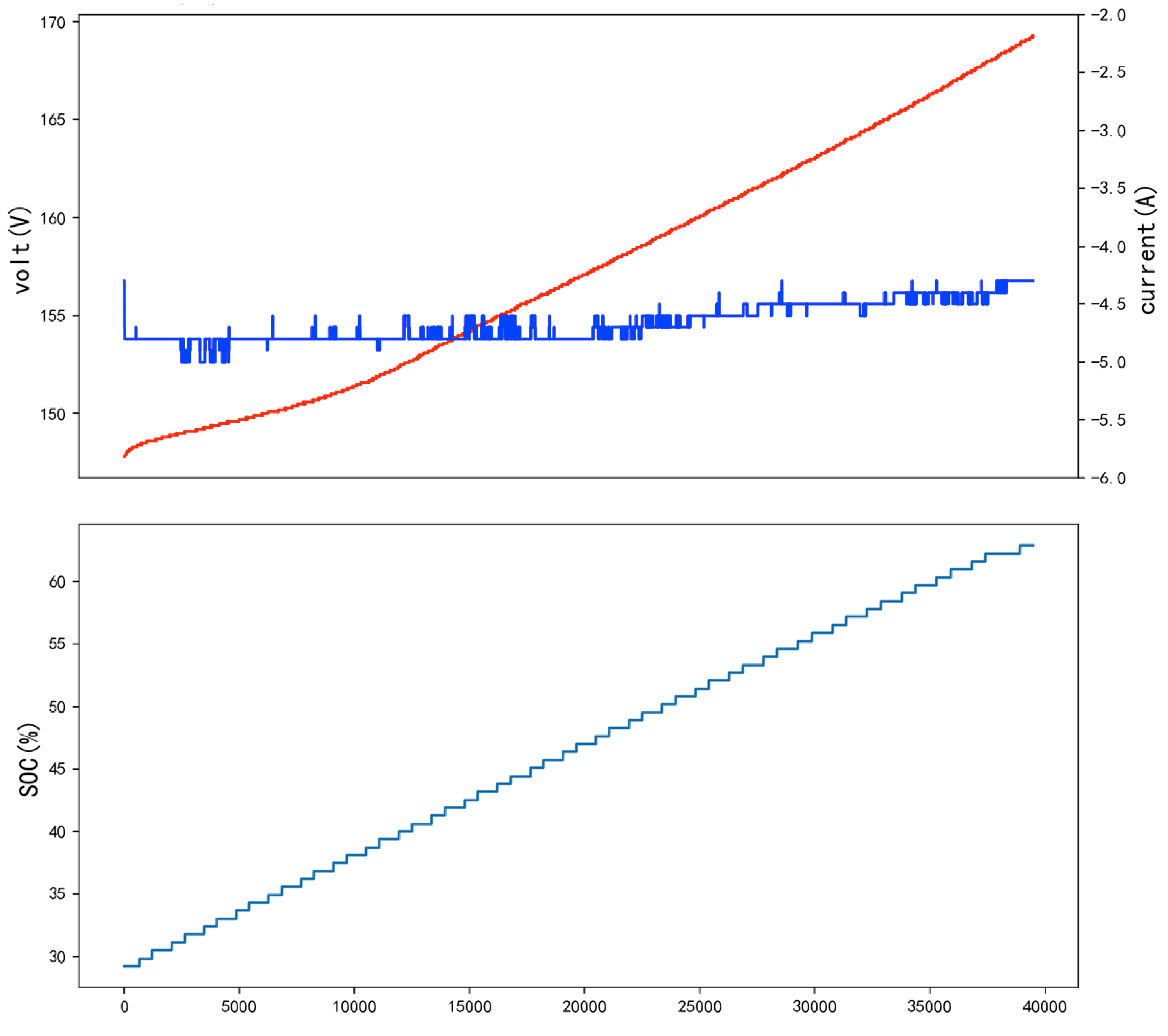
Battery Charging Detection Data. This dataset comes from Baidu PaddlePaddle Learning Competition: Energy AI Challenge - Anomaly Detection Track. It consists of processed data from full vehicle charging segments, aiming to analyze whether a vehicle is currently experiencing any faults based on charging data. The competition selected data that contains actual battery faults, but where the traditional alarm system failed to provide early warning. The data represents a mix of multiple vehicles of the same model. The charging segment data is relatively stable in new energy vehicle battery data, and the parameter changes in the battery follow a regular pattern. It is important to note that the data has been cleaned, and the raw values no longer reflect the characteristics of the battery itself, but the trend of the data changes still follows the battery’s regular patterns. The figure below illustrates the voltage, current, and SOC (State of Charge) changes over time during charging. The dataset is in .pkl file format, with each .pkl file containing a tuple (data, metadata). Each .pkl file corresponds to one battery and contains 28,390 samples. The shape of the data is (256, 8), with each column representing different features as shown in Table 1. The metadata contains label and mileage information. The label "00" indicates normal, and "10" indicates abnormal. The mileage indicates the total distance the battery has been used. The proportion of abnormal samples is approximately 17%.
Fall Detection Data. This dataset is a de-identified reconstruction of the dataset used in the paper by Kaluza et al. [16], and is currently hosted on Kaggle. The dataset consists of multiple CSV files, with each file recording the X, Y, Z position data of four sensors worn by different experimental subjects, along with time-point level anomaly labels, as shown in Table 2. Note that there is no timestamp feature in this dataset, as timestamps are often a key component in classification tasks. This can lead to an imbalance in learning tasks and limit the potential for broad generalization. The training set contains approximately 134,229 samples, with 5% of them being anomalous. The test set contains a total of 30,030 samples.
Figure 5.
Voltage, Current, and SOC Changes During Charging.
Motion State Recognition Data. This dataset comes from the preliminary round of the 2nd National Embedded Software Development Competition hosted by VeriSilicon. The dataset consists of multiple txt files, with each file recording 3-axis data (total of six axes) from the accelerometer and gyroscope of an intelligent wristband worn by different experimental subjects. The accelerometer and gyroscope data are sampled at a rate of 25 Hz. The accelerometer has a range of with a resolution of 4096/1G (one gravity is represented by the value 4096). The gyroscope has a range of with a resolution of 16.4/(1°/s) (one degree per second is represented by the value 16.4). The dataset includes six types of motions: walking, jogging, sitting, waving, squats, and jumping jacks. For jumping jacks, due to variations in the physical abilities of the data collectors, some files contain rest phases between actions (doing action -> rest -> doing action), where the subject remains still during the rest phase. This experiment only uses data for jumping jacks and jogging, containing 74,314 samples, with a balanced class distribution.
In this paper, AUC (Area Under the ROC Curve) is used as the evaluation metric. The ROC (Receiver Operating Characteristic) curve is a graphical representation of the classification model’s performance at different thresholds. It plots the relationship between False Positive Rate (FPR) and True Positive Rate (TPR). The confusion matrix for binary classification [18] is defined as:
| Actual Predict | Positive (P) | Negative (N) |
| Positive (P) | TP (TruePositive) | FN (FalseNegative) |
| Negative (N) | FP (FalsePositive) | TN (TrueNegative) |
Then, the formulas for calculating and are:
AUC is the area under the ROC curve, typically ranging between 0 and 1. The closer the AUC is to 1, the better the classification performance of the model. If the AUC is close to 0.5, it indicates the model’s performance is near random guessing, and if AUC is below 0.5, the model performs poorly. AUC is a robust performance metric for binary classification, especially in cases with imbalanced data, as it is unaffected by changes in the class distribution and provides a more stable performance evaluation standard. The AUC calculation method is as follows [17]:
3. Results
3.1. Comparison of Fixed Expression Weight Generation Function and Fixed Weight Ensemble Results
The ensemble of (SVM+MLP), (KNN+MLP), and (RF+MLP) learners was applied to the battery charging detection data, fall detection data, and motion state recognition data, respectively, where SVM is the Support Vector Machine model, MLP is the Multi-Layer Perceptron model, KNN is the K-Nearest Neighbors model, and RF is the Random Forest model. The AUC (Area Under the Curve) metrics were recorded for the single learner, three weight generation function ensembles, and fixed weight ensembles (the optimal weight distribution chosen from 1:9 to 9:1 for the fixed weight ensemble). The results are shown in Table 3..
As observed, on two imbalanced anomaly detection datasets, the ensemble of fixed expression weight generation functions significantly outperforms the single model results, as well as the fixed weight ensemble results. However, on the balanced dataset, although the fixed expression weight generation function ensemble performs better than the single model, it slightly lags behind the fixed weight ensemble. Therefore, the ensemble method based on fixed expression weight generation functions performs better for anomaly detection tasks with imbalanced classes. For balanced binary classification tasks, an adaptive learning method based on neural network-based weight generation functions should be used to optimize the ensemble.
3.2. Neural Network-Based Weight Generation Function
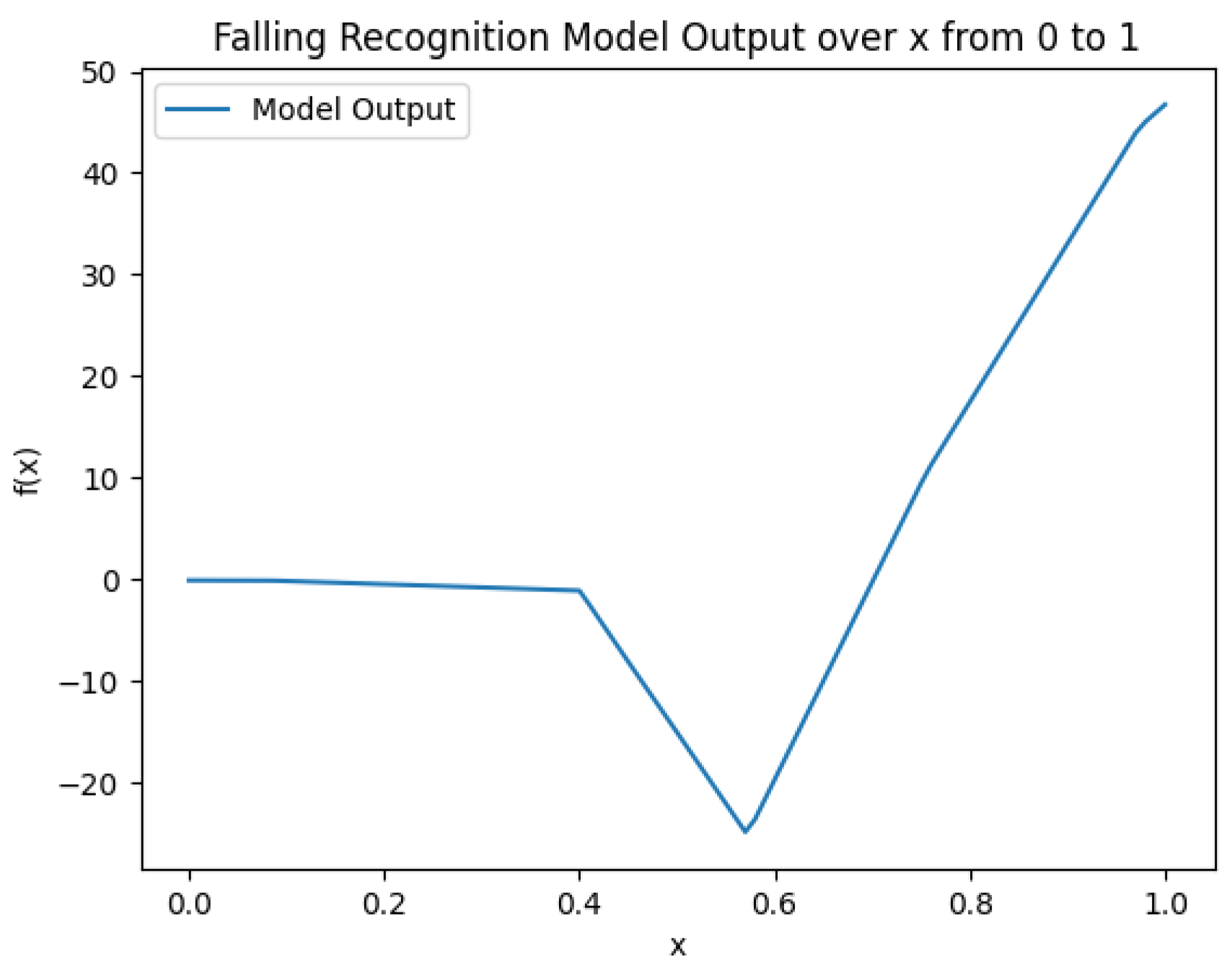
A simple FFN (Feedforward Neural Network) was constructed, with the structure shown in Figure 9, and fully trained based on Figure 4. The function images on the three datasets are shown in Figure 6 to Figure 8. Notably, for the "low at both ends, high in the middle" trend presented in fig:subfig1 and fig:subfig3, due to its value range being , we can factor out from both the numerator and denominator in equation eq:Fweightednormalized, effectively flipping the function graph, which is equivalent to the "high at both ends, low in the middle" trend. This experiment also proves the rationality of the ensemble strategy that assigns weights based on confidence levels.
Figure 6.
Neural Network-based Weight Generation Function on Battery Data.
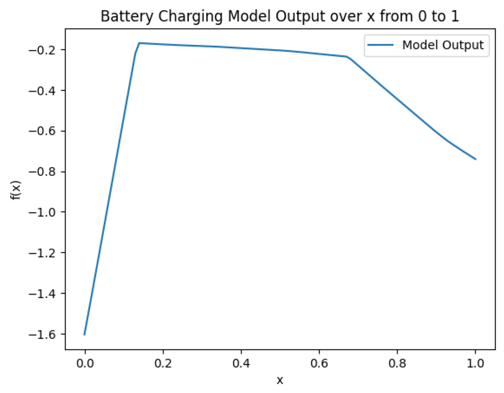
Figure 7.
Neural Network-based Weight Generation Function on Fall Data.
The ensemble results using the fully trained neural network-based weight generation function are shown in Table 4.. It can be observed that the neural network-based weight generation function performs better when dealing with balanced datasets.
Figure 8.
Neural Network-based Weight Generation Function on Motion Data.
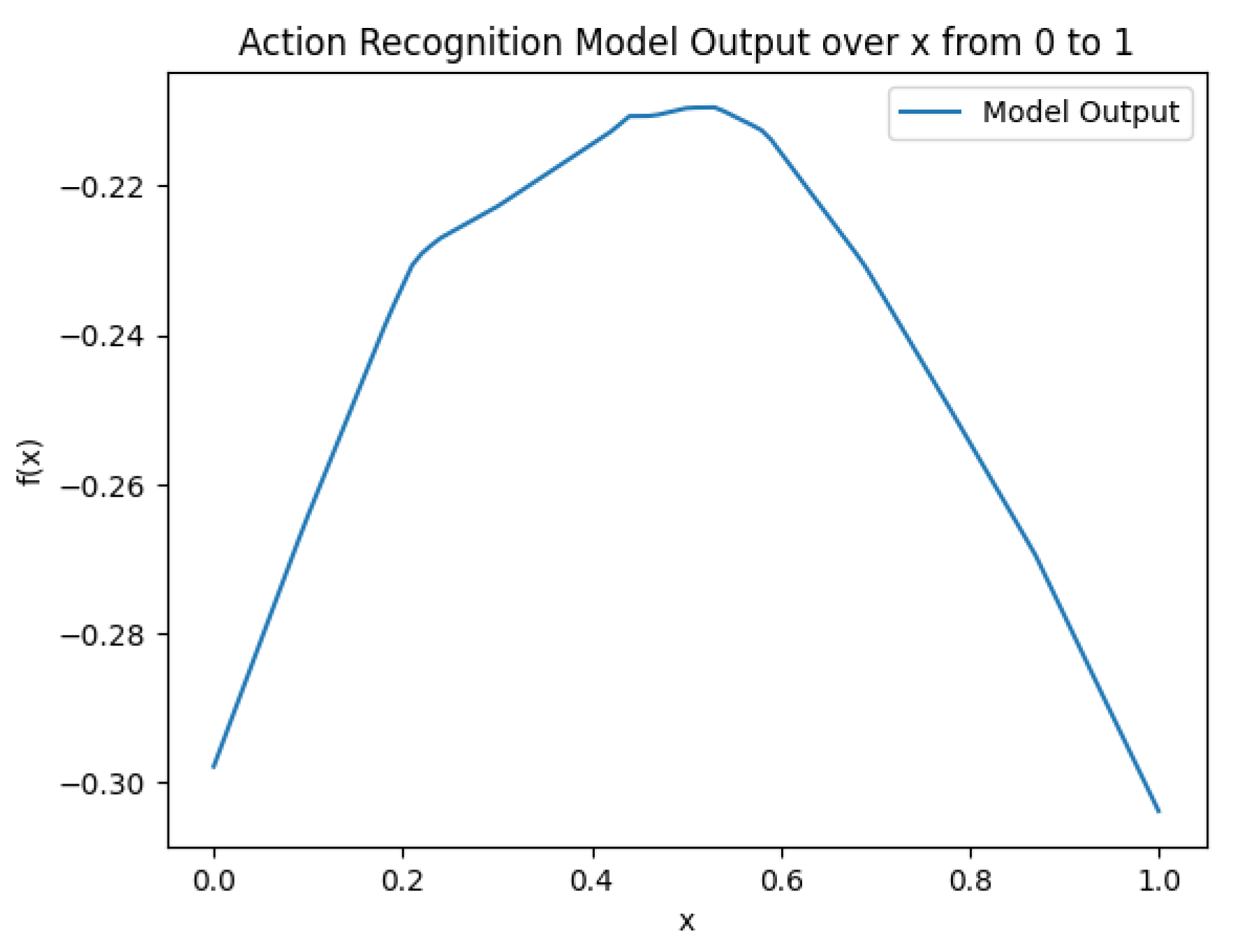
Figure 9.
Neural Network-based Weight Generation Function Structure.
4. Conclusions
This paper proposes a confidence-based weight generation function ensemble strategy for heterogeneous classifiers, which includes fixed function ensembles and neural network-based function ensembles. In the fixed function ensemble, three types of "high at both ends, low in the middle" functions are designed, demonstrating superior performance in imbalanced anomaly detection tasks. In the neural network-based function ensemble, an ingeniously designed neural network structure and loss function are used to adaptively learn the relationship between weight distribution and classifier outputs. On one hand, the neural network function ensemble exhibits a trend consistent with the "high at both ends, low in the middle" fixed functions, verifying the rationality of the proposed strategy. On the other hand, the neural network function ensemble outperforms the fixed function ensemble in balanced binary classification tasks, showcasing the great potential of this method.
The proposed strategy is currently applicable only to binary classification problems. Future work will explore its extension to multi-class classification tasks. Additionally, the neural network structure used in this paper is relatively simple and did not show particularly outstanding performance across the three datasets. Future research will focus on improving the network structure to achieve better ensemble results.
Author Contributions
Conceptualization, R.Q. and Y.Y.; methodology, R.Q. and Q.S.; validation, R.Q., Y.Y. and T.G.; investigation, R.Q.; resources, R.Q.; data curation, R.Q.; writing—original draft preparation, R.Q.; writing—review and editing, R.Q.; visualization, Y.Y.; supervision, Q.S.; project administration, Q.S. All authors have read and agreed to the published version of the manuscript.
Funding
This research received no external funding
Institutional Review Board Statement
Not applicable
Informed Consent Statement
Not applicable
Data Availability Statement
Data are contained within the article.
Acknowledgments
The authors are grateful to the Beihang University
Conflicts of Interest
The authors declare no conflicts of interest.
References
- Sesmero, M. P.; Ledezma, A. I.; Sanchis, A. Generating ensembles of heterogeneous classifiers using stacked generalization. Wiley Interdisciplinary Reviews: Data Mining and Knowledge Discovery 2015, 5, 21–34. [CrossRef]
- Odegua, R. An empirical study of ensemble techniques (bagging, boosting and stacking). In Proc. Conf.: Deep Learn. IndabaXAt; 2019.
- Wang, J.; Xu, H.; Liu, J.; et al. A bagging-strategy based heterogeneous ensemble deep neural networks approach for the multiple components fault diagnosis of hydraulic systems. Measurement Science and Technology 2023, 34, 065007. [CrossRef]
- Xia, Y.; Liu, C.; Da, B.; et al. A novel heterogeneous ensemble credit scoring model based on stacking approach. Expert Systems with Applications 2018, 93, 182–199. [CrossRef]
- Sobanadevi, V.; Ravi, G. Handling data imbalance using a heterogeneous bagging-based stacked ensemble (HBSE) for credit card fraud detection. In Intelligence in Big Data Technologies—Beyond the Hype: Proceedings of ICBDCC 2019; Springer Singapore: Singapore, 2021; pp. 517–525.
- Skalak, D. B. Prototype Selection for Composite Nearest Neighbor Classifiers; University of Massachusetts Amherst: Amherst, MA, 1997.
- Fan, W.; Stolfo, S.; Chan, P. Using conflicts among multiple base classifiers to measure the performance of stacking. In Proceedings of the ICML-99 Workshop on Recent Advances in Meta-Learning and Future Work; Ljubljana: Stefan Institute Publisher, 1999; pp. 10–17.
- Merz, C. J. Using correspondence analysis to combine classifiers. Machine Learning 1999, 36, 33–58. [CrossRef]
- Ting, K. M.; Witten, I. H. Issues in stacked generalization. Journal of Artificial Intelligence Research 1999, 10, 271–289. [CrossRef]
- Zefrehi, H. G.; Altınçay, H. Imbalance learning using heterogeneous ensembles. Expert Systems with Applications 2020, 142, 113005. [CrossRef]
- Zhao, Q. L.; Jiang, Y. H.; Xu, M. Incremental learning by heterogeneous bagging ensemble. In Advanced Data Mining and Applications: 6th International Conference, ADMA 2010, Chongqing, China, November 19-21, 2010, Proceedings, Part II; Springer Berlin Heidelberg: Berlin, Germany, 2010; pp. 1–12.
- Hsu, K. W.; Srivastava, J. Improving bagging performance through multi-algorithm ensembles. In Pacific-Asia Conference on Knowledge Discovery and Data Mining; Springer Berlin Heidelberg: Berlin, Germany, 2011; pp. 471–482.
- Nguyen, T. T.; Luong, A. V.; Dang, M. T.; et al. Ensemble selection based on classifier prediction confidence. Pattern Recognition 2020, 100, 107104. [CrossRef]
- Hu, J.; Shen, L.; Sun, G. Squeeze-and-Excitation Networks. In Proceedings of the IEEE Conference on Computer Vision and Pattern Recognition; IEEE: Piscataway, NJ, 2018; pp. 7132–7141.
- Rumelhart, D. E.; Hinton, G. E.; Williams, R. J. Learning representations by back-propagating errors. Nature 1986, 323, 533–536. DOI: 10.1038/323533a0. [CrossRef]
- Kaluza, B.; Mirchevska, V.; Dovgan, E.; Luštrek, M.; Gams, M. An agent-based approach to care in independent living. In Ambient Intelligence: First International Joint Conference, AmI 2010, Malaga, Spain, November 10-12, 2010. Proceedings 1; Springer Berlin Heidelberg: Berlin, Germany, 2010; pp. 177–186.
- Narkhede, S. Understanding AUC-ROC Curve. Towards Data Science 2018, 26, 220–227.
- Heydarian, M.; Doyle, T. E.; Samavi, R. MLCM: Multi-label confusion matrix. IEEE Access 2022, 10, 19083–19095. [CrossRef]
Figure 1.
Graph of the function .
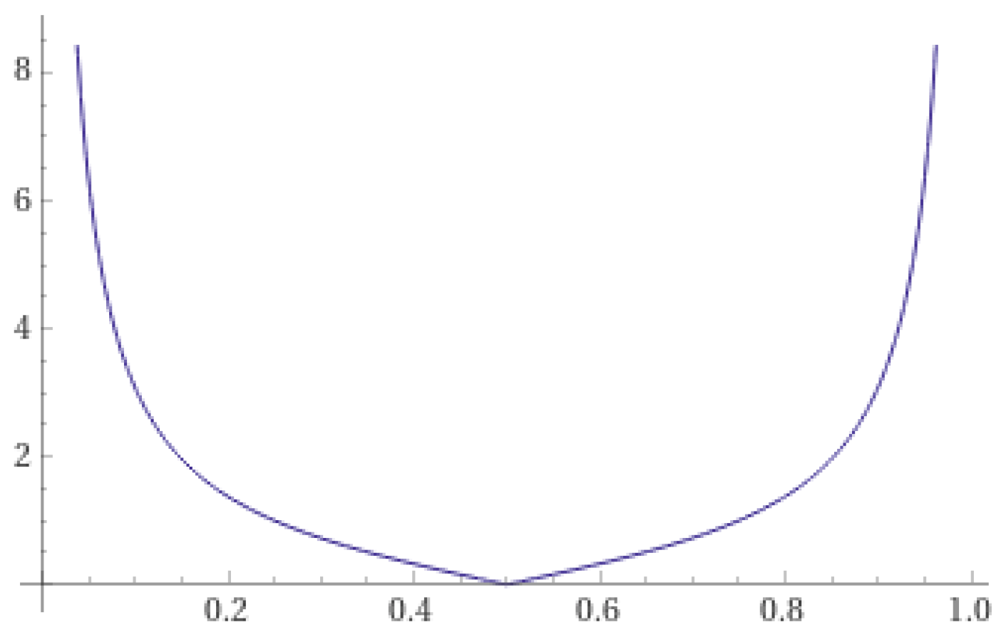
Figure 2.
Graph of the function .
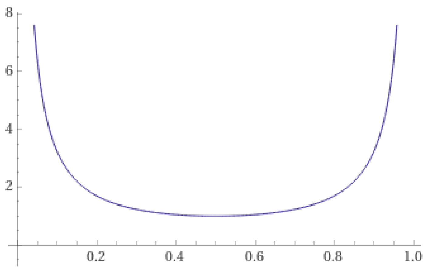
Figure 3.
Graph of the function .
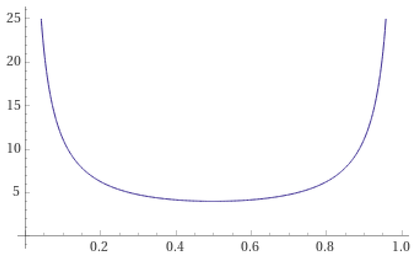
Figure 4.
Architecture of the Neural Network-Based Weight Generation Function.
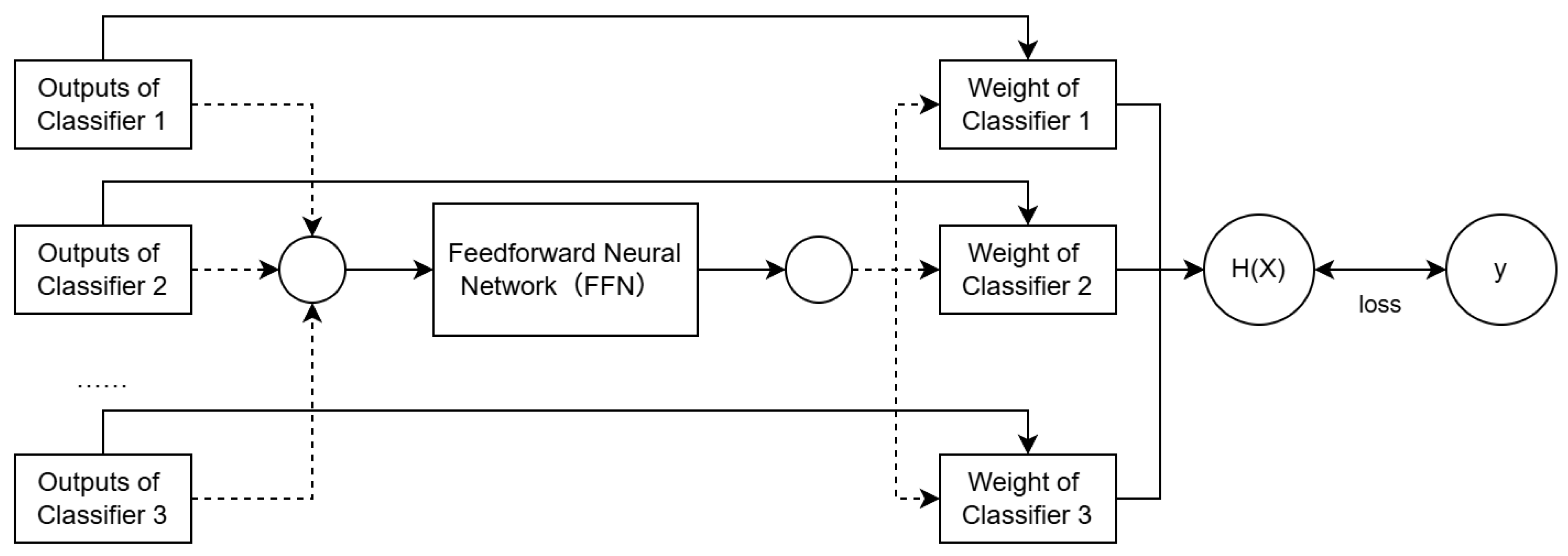

Table 1.
Battery Charging Detection Data Features and Their Meanings.
| Feature Name | Meaning |
|---|---|
| volt | Overall voltage |
| current | Overall current |
| soc | State of Charge |
| max_single_volt | Maximum cell voltage |
| min_single_volt | Minimum cell voltage |
| max_temp | Maximum temperature |
| min_temp | Minimum temperature |
| timestamp | Timestamp |
Note: These features are used to monitor and detect battery performance during the charging process.
Table 2.
Fall Detection Data Features and Their Meanings.
| Feature Name | Meaning |
|---|---|
| x | x-coordinate of the sensor |
| y | y-coordinate of the sensor |
| z | z-coordinate of the sensor |
| 010-000-024-033 | Sensor 1 data |
| 010-000-030-096 | Sensor 2 data |
| 020-000-032-221 | Sensor 3 data |
| 020-000-033-111 | Sensor 4 data |
| anomaly | Anomaly label (whether a fall occurred) |
Note: The data includes multi-axis sensor measurements to detect falls.
Table 3.
Experimental Results on Three Datasets.
| Dataset | SVM | MLP | KNN | RF | Fixed Weight Ensemble | Tan Function Ensemble | Sec Function Ensemble | Fractional Function Ensemble |
|---|---|---|---|---|---|---|---|---|
| Battery Data | 0.9366 | 0.9313 | * | * | 0.9441 | 0.9556 | 0.9558 | 0.9557 |
| Fall Data | * | 0.8168 | 0.8170 | * | 0.8353 | 0.8329 | 0.8375 | 0.8377 |
| Motion Data | * | 0.9806 | * | 0.9779 | 0.9883 | 0.9806 | 0.9855 | 0.9879 |
Table 4.
Experimental Results with Neural Network-based Weight Generation Function.
| Dataset | SVM | MLP | KNN | RF | Fixed Weight Ensemble | Fixed Function Ensemble | Neural Network Function Ensemble |
|---|---|---|---|---|---|---|---|
| Battery Data | 0.9366 | 0.9313 | * | * | 0.9441 | 0.9558 | 0.9545 |
| Fall Data | * | 0.8168 | 0.8170 | * | 0.8353 | 0.8377 | 0.8361 |
| Motion Data | * | 0.9806 | * | 0.9779 | 0.988332 | 0.9879 | 0.988339 |
Disclaimer/Publisher’s Note: The statements, opinions and data contained in all publications are solely those of the individual author(s) and contributor(s) and not of MDPI and/or the editor(s). MDPI and/or the editor(s) disclaim responsibility for any injury to people or property resulting from any ideas, methods, instructions or products referred to in the content. |
© 2024 by the authors. Licensee MDPI, Basel, Switzerland. This article is an open access article distributed under the terms and conditions of the Creative Commons Attribution (CC BY) license (http://creativecommons.org/licenses/by/4.0/).
Copyright: This open access article is published under a Creative Commons CC BY 4.0 license, which permit the free download, distribution, and reuse, provided that the author and preprint are cited in any reuse.


