Submitted:
19 December 2024
Posted:
23 December 2024
You are already at the latest version
Abstract
Fractal geometry provides a novel mathematical description that fits the chaotic nature of different phenomena. It was demonstrated widely that the benefits of the unique properties of fractal analysis are limitless. the concept of fractal dimension provided a perfect treatment of data on the architecture or dynamics of a certain system. This work aims to review the results of using this concept in analyzing different biological systems known for varying levels of complexity, beginning with analyzing architectures such as chromatin, cell membrane, cytoskeleton, and tissue arrangement, to the behavior of gene expression and brain activity, and then studying branching networks such as the blood, lymphatic, and neural networks. The results show that the use of fractal analysis represents a powerful tool in determining a unique signature for the system state, and whether it is healthy or diseased, in addition to distinguishing the type of disease and the possibility of using fractal modifications for therapeutic interventions, which makes fractal analysis a revolutionary tool.
Keywords:
factal theory
; fractal geometry
; chaos
; patterns
; complexity
; modifications
; fractal dimention
“Clouds are not spheres, mountains are not cones, coastlines are not circles, and bark is not smooth, nor does lightning travel in a straight line.” ― Benoît Mandelbrot
1. Introduction
1.1. The Fractal Geometry of Nature
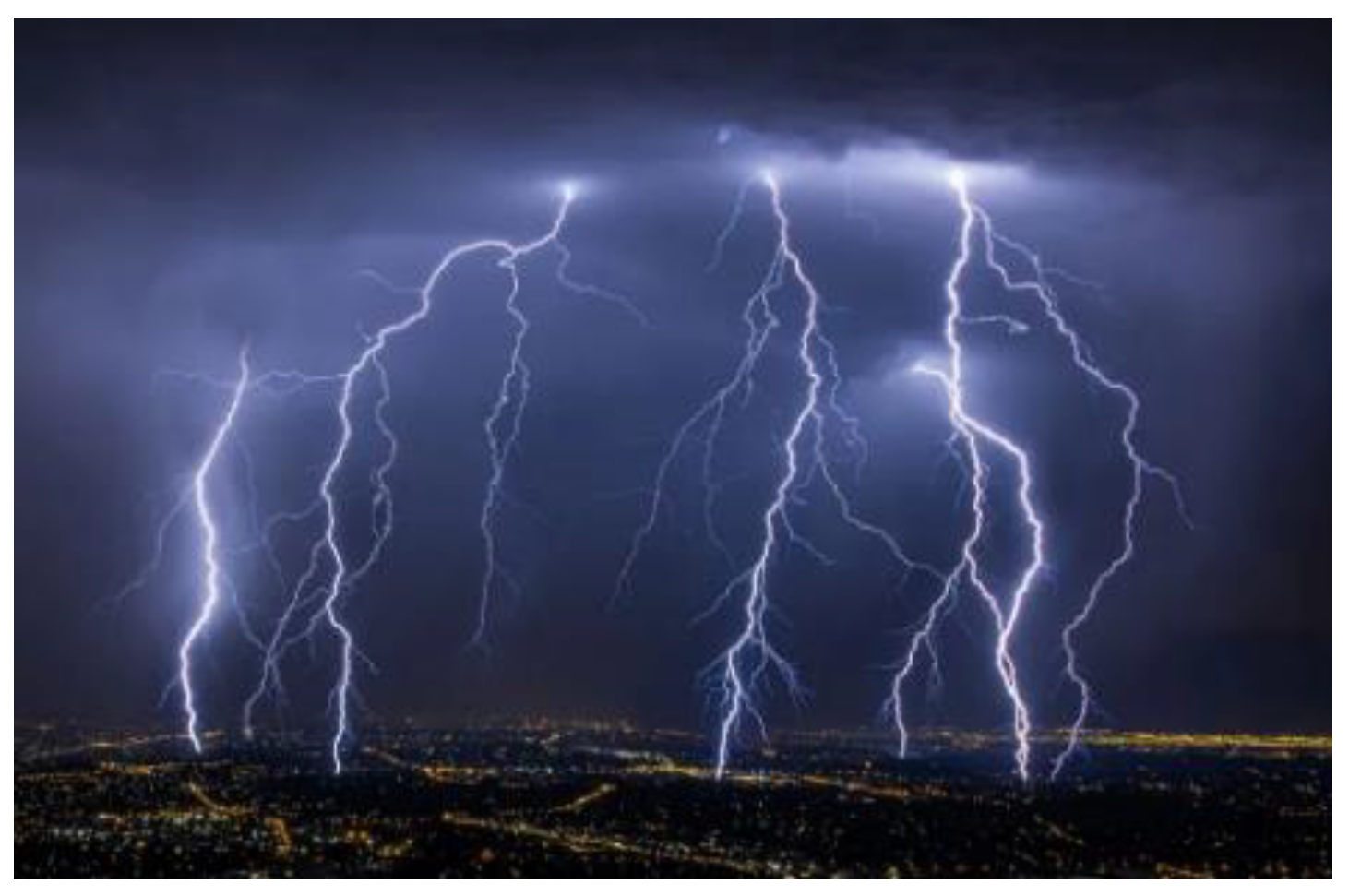
Fractal theory has provided a novel mathematical framework for dealing with the architectural complexity of nonlinear systems[1,2], which is what traditional Euclidean geometry failed to do. For example, when calculating the coastline length extending from one point to another, we see it as a set of a small straight line to reach an approximate value. Still, fractal geometry can describe the “roughness degree” of irregular surfaces such as coastlines, and river branches as shown in (Figure 1) or with mountain surfaces, cloud shapes, and Lightning lines in (Figure 2), and many other natural phenomena[1]. The relation between all these phenomena is that they show the same complexity pattern at different scales. For example, the pattern of the main branches of a river from its source to its mouth is like the pattern of its sub-branches between cities. Thus, the change pattern is constant whenever the observation scale is reduced.
Figure 1.
Rivers Tributaries (Google Earth).
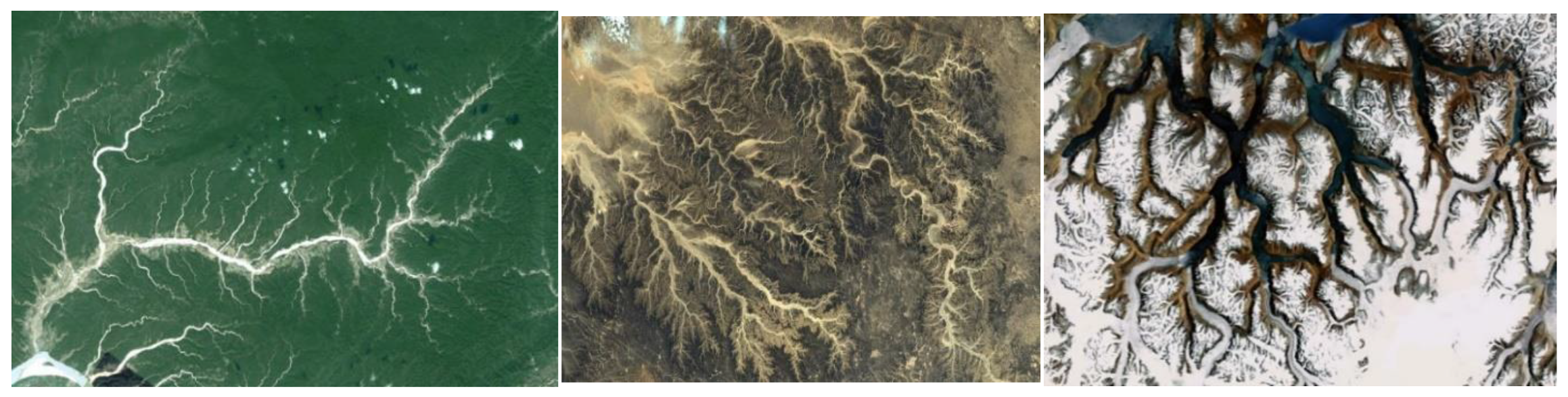
Figure 2.
Clouds.
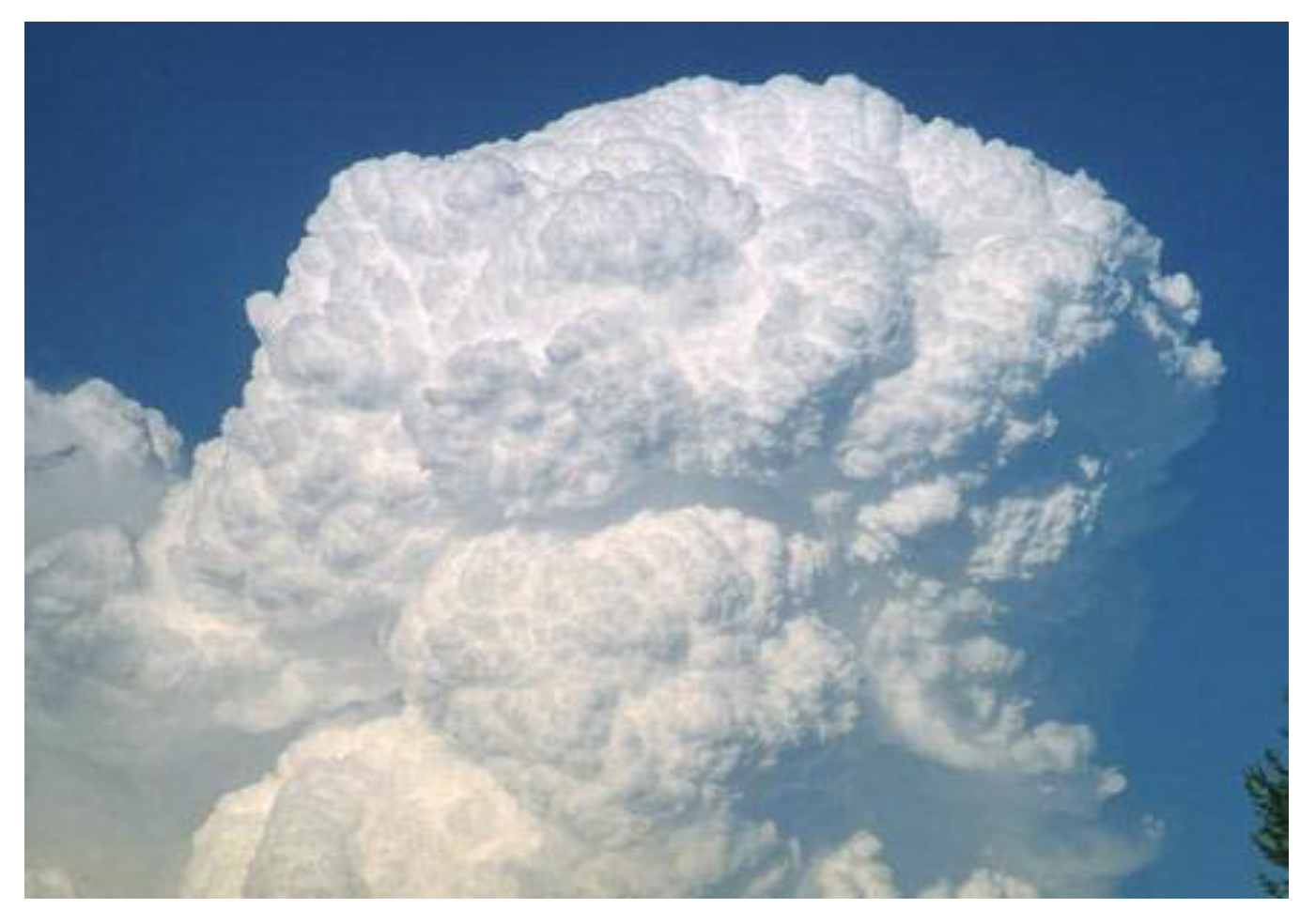
Figure 3.
Mountain Surface.

Figure 4.
Lighting Lines.
This property is known as “self-similarity”, which means that the shape or composition of the structure is repeated at different levels of observation[1]. This type of phenomenon is not only at the spatial level but also at the temporal level, as the change in financial markets), in which self-similar behavior appears at different time levels shown in (Figure 5 and Figure 6), which means that the pattern of change of the function at the years and months level is like its pattern of change at the level of weeks and days. All systems that exhibit self-similarity in their structural or behavioral composition can be described as “scale-free” or “scale-invariant” systems. Since fractal phenomena can’t be explained using integers, the degree of complexity is measured in fractional numbers through a mathematical quantity known as “fractal dimension”[1].
Fractal phenomena are divided into two main categories according to the order of each of them: deterministic fractal systems, and statistical fractal systems. each of which has its distinctive structure and method of measurement. Deterministic fractal systems shown in (Figure 7) are shapes and patterns that are generated mathematically and do not exist in nature because they are ideal in composition and can be infinite in scale such as the Sierpinski triangle (Figure 7b) and the Menger sponge (Figure 7c)[3,4]. As for statistical fractal systems shown in (Figure 8), they are used to describe the fractals of natural phenomena because they are not ideal, meaning that their composition at different levels does not exactly match the main shape and they cannot be finite due to physical limits[1,5,6].
1.2. Biological Fractal Pattern
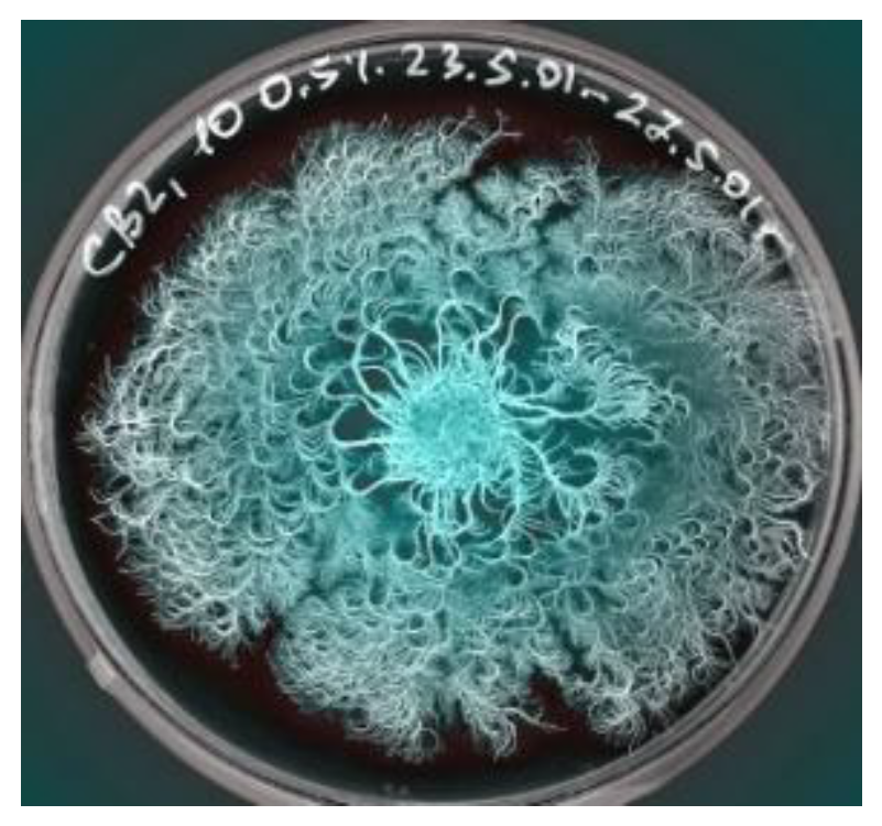
When viewing biological systems through the lens of fractal geometry[2,8], we find that many biological structures and dynamics exhibit clear fractal patterns[1,2,8], such as those shown by trees, in which the twigs resemble the main branches shown in (Figure 9) or patterns that require precision, such as the structure of the cauliflower plant, in which its small lobes resemble the larger lobes, and so on, In addition to the networks of branches within animals, such as the network of blood vessels (Figure 10), lymphatics, and nerve circuits (Figure 11). The growth structures of slime molds (Figure 12), bacteria (Figure 13), and algae (Figure 14) exhibit fractal patterns that change according to their state of interaction with their environment. Therefore, when analyzing the architecture and dynamics of biological systems fractally, we find that the life kingdom has a large natural fractal phenomenon, spatially and temporally, Which, by studying it, can be exploited, and the most important thing is to understand the physics behind the emergence of this type of phenomena.
1.3. Hiddin Fractal Dynamics
Fractal analysis has shown effective ability in phenomena detection by analyzing fractal data. In addition to various applications based on fractal architecture designs, due to the unusual properties that fractal design gives to the material, whether at the spatial or temporal level. The main purpose of this research is to take advantage of the uniqueness of fractal phenomena and understand the physics behind their behavior. Special concepts such as fractal calculus are used to understand the system’s complexity better. The challenge is to use fractal analysis to find the optimal modifications to be exploited geometrically. However, the lack of research has led to a delay in industrial production.
Before the chaos theory was established, it was impossible to distinguish between purely random and chaotic behaviors within a complex system. Due to the nonlinear nature of fractal geometry, it was used to re-analyze the data of many phenomena to discover the hidden fractal geometric structure. The power of fractal theory lies in distinguishing the heterogeneities between complex systems by analyzing data fluctuations[12]. In cosmology, fractal analysis was used to explore patterns of distribution in large-scale structures like galaxies, clusters, and superclusters as the Laniakea supercluster shown in (Figure 15). By using the fractal dimension D12–15within classifying galaxies close to us based on their images and placing a unique signature of each galaxy separately. In this way, the classification accuracy rate increased from 92% to 95%[14,15], as well By applying fractal analysis to the cosmic web network (Figure 16), which is a part of the universe’s large-scale structure, self-similar properties appear on multiple scales, showing a hidden multifractal distribution[13].
Earthquakes are one of the most complex geophysical phenomena and understanding their organizational structure remains one of the challenges facing modern science[16,17]. It has been observed that the spatial-temporal distribution of earthquakes shows the scale-invariant property[16,17,18,19,20]. By analyzing the time series of seismic waves (Figure 17), the statistical fractal distribution of earthquakes was shown, but with local correlations that differ from global ones[16]. There is no doubt that a correlation exists between the earthquake intensity and its “roughness”, i.e., the increase in its fractal dimension[17,20]. Accordingly, the earthquake and aftershock waves can be classified based on their fractal dimension changes[16,18,20].
Recently, time series of solar magnetic fields have been analyzed using a novel visualization method called Gaussianity Scalogram. The results show that the temporal distribution of the solar surface magnetic fields exhibits fractal-like patterns on different time scales ranging from years to seconds as appearing in (Figure 19). By analyzing “chaotic” data for other phenomena, we must ask about hidden fractal structures around nature[21].
Figure 18.
Parker Solar Prope (Nasa).
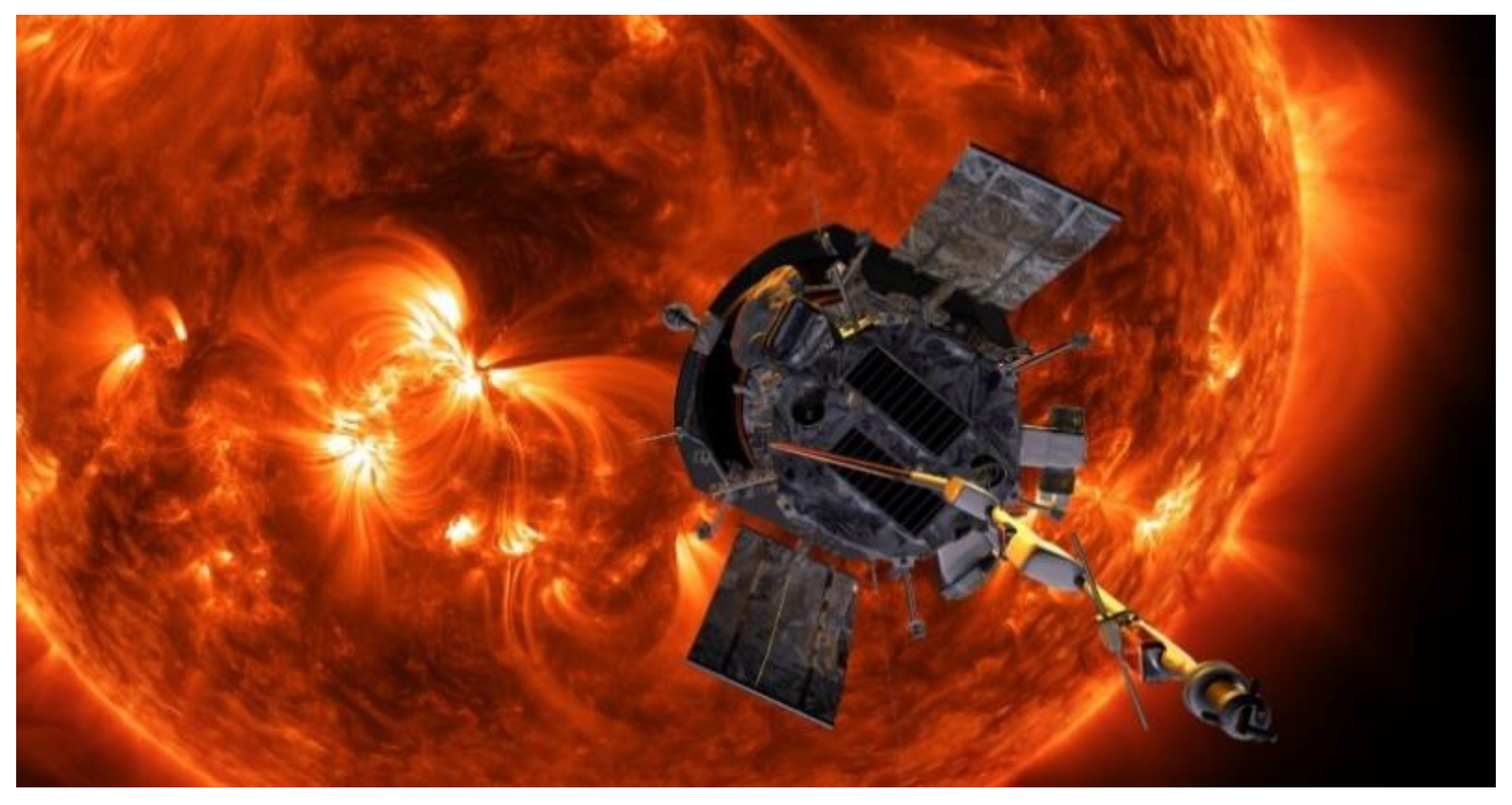
Figure 19.
Hierarchic multiscale time structrue[21].
Figure 19.
Hierarchic multiscale time structrue[21].
1.4. Fractal-Based Modifications
Fractal architecture-based designs have unique properties, as they get the material special behaviors that don’t appear when applying other traditional designs[5,22]. In addition, the special capabilities of fractal modifications occur without change to the material’s chemistry or physical state. The fractal structure can be applied at the level of structural modifications such as antennas[23,24], grid filters[25], supercapacitors[26], or metamaterials[22,24], or at the level of temporal modifications such as using pink noise to simulate biological signals[27,28], where promising results appear with system efficiency versus energy consumption. So far, no principle theory explains why fractals have these unique properties. Self-similarity is the secret key, thus Fractal design gives a wide range of selections for industrial production [22,29].
When using the self-similarity approach in antenna designing, as shown in (Figure 20), we see a significant improvement to traditional antenna features, such as smaller size, lower weight, operation in multiple frequency bands, and working efficiency. Fractal antennae have been used in industrial fields widely due to their compact size, lower price, and ease of fabrication (Figure 20j,k), there are various antenna shapes based on their fractal dimension which gives the ability to design based on specific properties [22,24,30,31]. A recent promising use of a fractal antenna is with biosensor applications, a recent results show that fractal design, shown in (Figure 20l) has a high sensitivity to low fructose concentrations with miniaturized dimensions and low manufacturing cost compared with other designs[32].
Many natural structures, such as bone, shells, and wood, have mechanical robustness and damage tolerance to their fractal-like architecture. Fractal hierarchical design principles are applied to 3D hierarchical nano-lattices of hollow alumina made of self-similar cells on different orders. Measurements show that after compression to ≥ 50% strain, alumina samples recover up to 98% of their original height. Still, there is an order limit because the additional orders of hierarchy after the second one (Figure 21) don’t show an increase in strength or stiffness. These results must improve industrial applications due to their unique properties as ultra-light weight, and recoverability, which outperform existing traditional designs of nanomaterials [33].
Figure 21.
SEM images of the various second-order samples. (Scale bars: 20 μm.)[33].
Figure 21.
SEM images of the various second-order samples. (Scale bars: 20 μm.)[33].
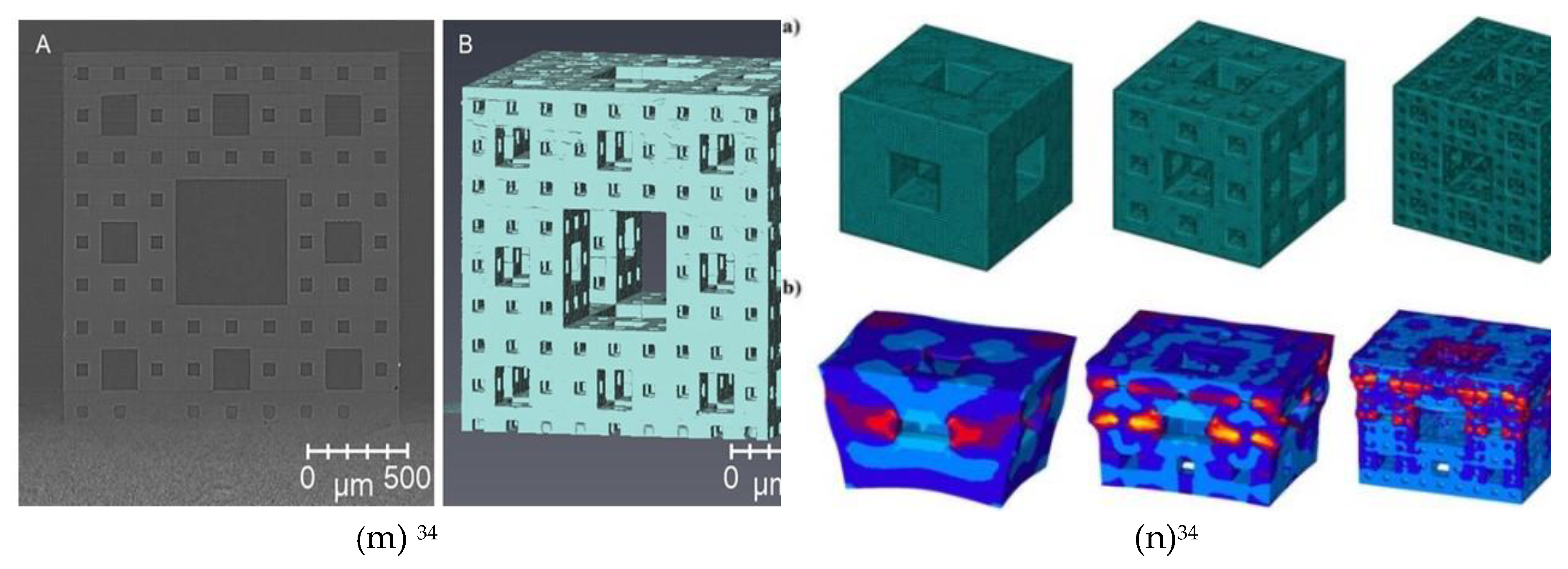
Porous polymers which are fractal-architectured and arranged < 100 μm apart, showed unique properties in increasing the ability to dissipate the shockwave stress and wave velocity of energy. By firing an impactor into them at approximately 670 mi/h, The fractal-structured cubes dissipated the shocks five times better than solid cubes of the same material and physical conditions. This ability is provided due to its “critical” packing ratio designed by the self-similarity (Figure 21m). The higher the order of iterations, the more energy dissipating the cube is due to the increased number of small gaps (Figure 21n), This is a new design feature to handle shock and rebound vibrations [34].
Figure 21.
(m) 3D Menger Sponge Cube, (n) Temperature distribution in the Menger structure following shockwave.
Figure 21.
(m) 3D Menger Sponge Cube, (n) Temperature distribution in the Menger structure following shockwave.
The disturbance density in a medium can be controlled by using a fractal grid that intercepts the current. Simulation of a fractal square grid with three successive iterations (Figure 22.) has shown that as the grid fractal dimension increases, the density of disturbance transmission along the path behind the grid increases (Figure 23.). By applying different fractal designs with certain dimensions, spatial regulation of the disturbance density can be obtained depending on the type of design and its fractal dimension [34].
One promising modification is to study the effect of fractal patterns in solar cell design on light absorption efficiency. Simulation experiments and some experimental results have shown that fractal designs enhance solar cell efficiency, with an improvement factor of up to 83.4% when using a 50 nm thick silicon film with a silver back reflector as a reference structure. The presence of fractal self-similar structure of the Ag layer shown in (Figure 24) leads to various momentum compensations in the system, which allows the incident light at different frequency ranges to be coupled with cavity and surface plasmon modes, thus resulting in broadband light absorption, which enhances the efficiency range (Figure 25) of the solar cell. This architectural addition contributes to developing high-performance plasmonic solar cells or designing integrated photovoltaic devices [35].
2. An Overview of The Fractal Geometry History
Fractal geometry has been passed through many stages of insightful observations and mathematical developments through a series of contributions. By the late 18th century, the German physicist Georg Christoph Lichtenberg (1742 – 1799) shown in (Figure 26) made significant strides in the study of fractal systems through his work on electrical discharges. Lichtenberg’s experiments involved high-voltage electrical discharges on dielectrics, which resulted in the formation of intricate, tree-like patterns known today as Lichtenberg figures (Figure 27). These patterns, characterized by their self-similarity at different scales, which are very close to lighting lines or tree branches, provided some of the earliest visual evidence of spatial fractal structures in natural phenomena. Fast forward to the 19th century, Karl Weierstrass (1815-1897) shown in (Figure 28), a German mathematician, further advanced the understanding of fractal systems through his rigorous mathematical work. Weierstrass constructed a function that was continuous everywhere but differentiable nowhere, known as the Weierstrass function (Figure 29). This groundbreaking example is the first of a deterministic function that challenged the traditional notions of smoothness and continuity to its fractal nature. Lichtenberg’s empirical observations and Weierstrass’s theoretical advancements marked the beginning of an enduring scientific exploration into the fractal’s complexity. Their pioneering efforts opened new avenues for understanding the intricate patterns that emerge in nature and set the stage for future discoveries in the field [6,36].
The most important developments of fractal geometry are within the early mathematical construction, which is represented in the work of pioneering mathematicians, such as Georg Cantor (1845-1918), Gaston Julia (1893–1978), and Benoît Mandelbrot (1924–2010). The first fractal model was created by Cantor (Figure 30), who was working on the concept of infinite sets and the construction of the Cantor set (Figure 31), which is often cited as a foundational fractal, is created by repeatedly removing the middle third of a line segment, leaving behind an infinitely complex structure that retains its key properties regardless of the scale. This work not only illustrated the counterintuitive nature of infinite processes but also introduced ideas of self-similarity, a hallmark of fractals [36].
Gaston Julia (Figure 32) made remarkable contributions to the study of fractals through his work on iterative functions and complex dynamics. In the early 20th century, Julia analyzed the behavior of complex functions when iteratively applied, leading to the discovery of intricate and self-referential structures known today as Julia sets (Figure 33). These sets exhibit infinite complexity and striking beauty, showcasing patterns that vary dramatically based on the function and initial conditions. Julia’s research, published in 1918, introduced key concepts in what would later become fractal geometry [36].
The modern era of fractal theory begins with Benoît Mandelbrot (Figure 34), often called the “father of fractal geometry”, revolutionizing mathematics and science by formalizing and popularizing the concept of fractals. Mandelbrot introduced the term “fractal” in 1975 derived from the Latin word “Frāctus” which means “cracked” or “rough”. This is the first time using fractal geometry in describing fragmented shapes that exhibit self-similarity across different scales. His most famous contribution during his work at IBM, the Mandelbrot set (Figure 35), visualizes the behavior of a simple complex function under iteration, revealing a boundary of infinite complexity. Mandelbrot demonstrated how fractals could model natural phenomena where traditional Euclidean geometry falls short. His intrinsic observation is represented in his famous quote “Clouds are not spheres, mountains are not cones, coastlines are not circles, and bark is not smooth, nor does lightning travel in a straight line”.His seminal book, The Fractal Geometry of Nature, published in 1982, showcased the practical and theoretical applications of fractals. Mandelbrot’s work bridged the gap between pure mathematics and real-world complexity, reshaping how scientists understand patterns and chaos in nature which opened the door to a novel mathematical framework for analysis [36,37].
The contributions of other mathematicians such as Helge von Koch (1870 –1924), Wacław Sierpiński (1882- 1969), Paul Lévy (1886-1971), and Karl Menger (1902-1985) significantly enriched the field of fractal geometry, each introducing unique constructs that highlighted the intricate properties of fractals. Their work focused on deterministic fractals, which are idealized, meaning they don’t have the chaotic parameters that make the shape appear random like natural systems, such as the rugged surface of mountains. They are also infinite; the higher the zoom scale, the more sub-patterns appear without stopping.
Helge von Koch (Figure 36) introduced the Koch snowflake (Figure 37), a curve created by successively adding equilateral triangles to each segment. This curve has an infinite perimeter yet encloses a finite area, illustrating fractals’ ability to challenge conventional notions of geometry. Wacław Sierpiński (Figure 38) developed the Sierpiński triangle (Figure 39), which is formed by recursively removing the central triangle of an equilateral triangle, producing a pattern with zero area but infinite perimeter. The French mathematician Paul Lévy (Figure 40 ) studied stochastic processes and geometric constructions. Lévy’s work on self-similar patterns and random processes laid the foundation for many later developments in the field. One of his notable contributions is the Lévy C curve (Figure 41), which is created by repeatedly replacing each straight line segment with a specific pattern of two segments forming an isosceles triangle, resulting in an infinitely intricate, non-differentiable curve. In the early 20th century, Karl Menger (Figure 42) developed the Menger sponge (Figure 43), a three-dimensional fractal constructed by recursively removing the central cube from each face. This structure has zero volume but infinite surface area, extending fractal concepts into three dimensions and influencing topology. Together, these mathematicians paved the way for modern fractal geometry, showcasing the elegance of infinite complexity through iterative processes and self-similarity. Their constructs continue to serve as fundamental examples in the study of fractals and their applications [36].
3. Fractal Dimension Concept
Traditional Euclidean geometry deals with shapes with an integer dimension such as a point with D = 0, a straight line with D = 1, a square with D = 2, and a cube with D = 3. It cannot deal with shapes or bodies that have a fractal nature, as they can only be described through fractions such as D = 1.32, 1.56, 1.78, and so on. Therefore, a set of computational methods has been developed to measure the complexity or roughness of a surface, such as the box-counting method, the Hausdroff dimension, and the Mass-radius method, all of which aim to determine the heterogeneity degree of the system, which has a unique fractal dimension. Fractals are divided into two main types: deterministic fractals with an ideal and infinite structure, and statistical fractals, which distinguish natural fractals - physical and biological - and each has its specific methods. As for mathematical deterministic fractals, it can be said that they are determined according to two things: the fractal order and the fractal dimension. The fractal order is the type of change or distortion that the shape or system is exposed to in general as shown in the second column of (Figure 44). In contrast, the fractal dimension is a measure of the number of iterations that have occurred on different scales as shown in column 3,4, and 5 in (Figure 44), where the number of self -similar iterations is proportional to the fractal dimension of the shape [36,38].
3.1. Box Counting Method
This method is one of the most used techniques for determining the fractal dimension of objects that exhibit self-similarity or irregularity at different scales. The process involves covering the object with a grid of boxes -squares in 2D or cubes in 3D- of a certain size and counting how many of these boxes intersect the object. By reducing the size of the boxes and observing how the number of intersecting boxes changes, the fractal dimension of the object can be estimated, providing a quantitative measure of its complexity represented in fractional ratio. Mathematically, the box-counting dimension is defined by analyzing the scaling behavior of the number of boxes required to cover the fractal as the box size decreases. The relationship is expressed as:
The practical implementation involves plotting log (1/∀), where the slope of the resulting linear graph provides an estimate of the fractal dimension D. One of the old problems was the problem of measuring the length of the coast of Britain, because of the winding nature of the coast, the correct length could not be calculated because every time the measurement was made with a smaller longitudinal scale, we found that the length increased. Therefore, by using a grid of squares that fill the borders and whose area becomes zero, the degree of irregularity can be calculated as shown in (Figure 45). This process revealed a fractal dimension of approximately D = 1.25, indicating that the coastline is more complex than a straight-line D = 1, but less complex than a filled plane D = 2. The value reflects the intricate, self-similar structure of the coastline at different scales [36,38].
4. Fractal Analysis within Theranostics
Over the past four decades, fractal analysis has been applied to various natural systems, both physical and biological. It is known that the organizational nature of biological structures has a special nature, as they are divided into several cognitive levels, where there are the subcellular, cellular, tissue, organic, and systemic levels, in addition to the environmental level known as collective intelligence, each of which has its physical morphology at the spatial structural level and the temporal behavioral level. The results of the analysis of architectural and temporal patterns of various biological systems showed a broad fractal behavior. By comparing the fractal dimensions of different states of the same system, it is possible to determine the states of health and disease, and it may even reach the point of knowing the type of disease and determining its degree. Biological systems are characterized by having patterns that represent the stable state, and once they deviate from them, the amount of distortion can be estimated and interpreted based on previous data. For example, when the fractal dimension increases or decreases from a certain range as shown in (Figure 46), this means that there is a structural or behavioral change in the system that is different from its nature. Therefore, the fractal dimension can be used as a powerful predictive tool before traditional diagnostic tools. Ease of application, widespread use, low cost, and accuracy of results are all reasons that make fractal analysis a primary tool in making critical medical decisions in the future, especially with the integration of tools such as AI and machine learning [5,28,39].
4.1. Cell Chromatin
Chromatin, a mixture of DNA and proteins, has a very complex structure. Fractal analysis shows that chromatin exhibits a fractal spatial-temporal organization. Spatial organization refers to the three-dimensional arrangement of chromatin within the nucleus. It has shown that chromatin doesn’t fold randomly but exhibits fractal spatial patterns. Modeling has shown that the advantage lies in its structure, known as a “Fractal globule” shown in (Figure 47) which allows a large amount of DNA to be condensed into a small space while maintaining access to genetic information when needed[40]. Temporal organization is the changes of chromatin dynamics, while by analyzing gene expression data, we find that these temporal changes can also exhibit fractal behavior. An increase in fractal dimension can indicate an increase in heterogeneity of chromatin density (Figure 48) The fractal dimension of chromatin has been found to increase in cancer cells. For example, a study found a significant increase in fractal dimension in patients with precancerous colon adenomas compared to patients without these tumors. In another study of cervical cancer cells, the fractal dimension of chromatin was found to increase from (D = 1.02) in normal cells to (D = 1.32) in cervical dysplasia stage I (CIN1), (D = 1.37) in CIN2, and a peak of (D = 1.40) in CIN3[41]. The relationship between fractal chromatin organization and gene expression is a promising area of research. Changes in the fractal dimension of chromatin can lead to changes in DNA accessibility, affecting gene expression. This could lead to new diagnostic and therapeutic tools that target chromatin organization to treat diseases [40,41,42,43].
4.2. Cell Surface
Fractal analysis is important in understanding cell surface morphology and its changes based on certain abnormalities. The importance of measuring the surface fractality lies in revealing the complexity of the cells. Based on the cell fractal dimension, we determine whether it is in a normal or pathological state and at what stage. Studies show that cancer cells are characterized by an increase in the fractal dimension of their surface compared to normal cells shown in (Figure 49). This property can be used to distinguish cancer cells from normal cells within the same tissue with high efficiency, a study found that the fractal dimension of malignant pancreatic cancer cells was higher than the fractal dimension of benign pancreatic cancer cells. The higher fractal dimension in cancer cells is attributed to the increased surface roughness, such as the formation of appendages and tortuous membranes. Studies have shown the possibility of using nano-surfaces with fractal dimensions targeting cancer cells with high efficiency. Nano surfaces with appropriate fractal dimensions (Figure 50), coated with specific antibodies, can be used to capture and separate cancer cells from blood samples efficiently; by designing surfaces with specific fractal dimensions (D = 2.40-2.70), these surfaces showed a high ability to capture breast cancer cells (MCF7) due to their similar fractal dimensions [44,45,46,47,48,49].
4.3. Tissue Arrangement
It is known that cells have different types of communication between them within tissues, but we still haven’t much knowledge about their growth patterns organization, and their assembly with each other. A study has shown how mammary epithelial cells form multicellular clusters with a fractal, branch-like structure when cultured in a medium containing low concentrations of epidermal growth factor (EGF). The cell clusters exhibited a fractal dimension D = 1.74 ± 0.03. When analyzing the temporal growth of clusters, central cells known as leader cells appear at the periphery of the clusters, and their number increases with cluster size. For example, small clusters containing less than 10 cells are usually associated with only one leader cell. Larger clusters, consisting of 10 to 30 cells, are associated with two or more leader cells, which exhibit directed movement, where actin filaments extend in a specific direction, enabling them to pull neighboring cells behind them based on some cell-to-cell contacts. The collective coordination of the leader cell’s movement forms a larger interconnected network like a tree trunk with its branches network. This study demonstrated that the growth patterns of breast epithelial cells with a fractal structure (Figure 51) show a remarkable resemblance to diffusion-limited aggregation of nonliving colloidal particles. These findings prompt intensified research behind the biophysical processes that may play an important role in regulating tissue formation [50].
4.4. Branching Networks
Despite the enormous diversity of the life tree, there are some principles of system morphology that evolution hasn’t affected at all, such as the branching pattern of distribution networks within an organism. Distribution systems have maintained their fractal structure, which maximizes their efficiency, as they provide the largest possible area of influence relative to the total size of the network. Fractal analysis helps analyze different deformations based on their fractal dimension deviation from their normal range, such from the circulatory system which has a fractal dimension range (D = 1.6-1.9) (Figure 52a), to the lungs (D = 1.8-2.2) (Figure 52b), kidneys (D = 1.7- 2.0) (Figure 52c), and nervous system (D = 1.4-1.6) (Figure 52d), all of them can be treated as a non-linear distribution model. For example, finding an increase or decrease in the fractal dimension of the retinal blood vessels can indicate diseases such as diabetic retinopathy and cerebrovascular disease. Using fractal dimension to understand the adaptation mechanisms to their environment and finding varieties between species and even between different brain regions. It has been observed that there are differences in the fractal dimension of the bronchi between different mice species, indicating a genetic influence on the individual’s branching architecture, which means the fractal dimension can be considered a unique signature of an individual. These results prove that fractal analysis is a powerful tool for detecting morphological abnormalities, which helps to understand how biological systems are affected by diseases [51,52,53].
4.5. Radiomics
Fractal analysis plays an increasingly important role in radiomics, where it is used to assess the complexity of shapes and patterns in medical images. When analyzing brain imaging data as a model for comparing its diagnostic fractal measurements, FD values are found to be significantly higher in atypical meningiomas (grade II) with a (D = 1.58) than in benign tumors (grade I) with (D = 1.10), with tumors with higher malignant grades showing larger fractal dimensions due to irregularity of their edges (Figure 53). Changes in the complexity of brain structures resulting from aging or degenerative diseases can be distinguished by their fractal dimensions. For example, FD values have been observed to decrease in the gray matter of the brain with age and in Alzheimer’s disease, reflecting a loss of complexity in the brain structure. The specific morphological changes of each disease reflect a change in its degree of complexity (Figure 54). These differences help to distinguish between different diseases and determine their progression. Fractal analysis is therefore a promising tool, providing unique identification of tissue complexity that traditional methods don’t. It is expected that by combining the capabilities of AI with fractal analysis, diagnostic accuracy, and treatment guidance will increase in the future [54,55,56,57].
4.6. Physiological Signals
Fractal analysis is applied to complex biological time-series of organ activities, revealing hidden patterns and relations in the data that may not be apparent using traditional methods. A higher fractal dimension can indicate more complex fluctuations at different temporal scales. For example, the activity of a healthy heart may show a deviated fractal dimension than the activity of a diseased heart. Biological time series exhibit a property known as scale-invariance, meaning that the system exhibits fractal behavior and remains similar regardless of the scale at which it is analyzed as shown in (Figure 55). Instead of calculating just averages, individual variations are interpreted to understand how they relate to each other. These changes can reveal important information about the organ’s health, as random changes may indicate a loss of complexity and organization. For example, by analyzing ECG data, we can distinguish between normal and abnormal heart conditions, as loss of complexity in heart rate is associated with dysfunction. In addition, EEG analysis is important for understanding brain multiple functions, as the fractal properties of sensory signals are important for normal brain development. Distortion in the fractal structure of signals can lead to brain function loss and reduced adaptive plasticity. Analysis of brain activity of schizophrenia patients shows lower fractal dimensions compared with normal cases (Figure 56), reflecting a decline in the complexity and dynamic organization of the diseased brain. In normal cases, brain activity shows a certain fractal complexity, while in cases of schizophrenia - or other neurological disorders-, this complexity may be reduced, especially in brain networks affected by this disease. This difference in FD reflects changes in brain dynamics that could be a significant biological marker for schizophrenia. Undoubtedly, applying fractal analysis to other time series can distinguish many diseases and their symptoms by linking traditional diagnosis to the behavior fractal dimension [58,59,60,61,62].
5. Discussion
Numerous studies in biomathematics have concentrated on leveraging the fractal characteristics of biological systems. Chaos theory has introduced a nonlinear mathematical approach that is well-suited for addressing both physical and biological systems, challenging the earlier assumption that nonlinear data is entirely random and that no useful insights can be gleaned from such data. Over the last forty years, fractal theory has yielded significant findings regarding fractal analysis, uncovering concealed phenomena, and applying modifications to fractal structures in numerous models, which have demonstrated their effectiveness compared to more traditional designs, potentially transforming the industry shortly. Biological systems across various levels—cellular, tissue, and more—exhibit considerable diversity; however, each system possesses a unique hidden structure that encapsulates the importance of fractal analysis in comprehending that structure and in developing new medical capabilities. By analyzing data from biological systems, we can distinguish between different species as well as between healthy and diseased states, and in cases of malfunction, we can also determine the disease and its progression, all through a straightforward idea such as the fractal dimension. The future of fractal geometry is focused on uncovering theories that link fractal occurrences in diverse systems, aiming to investigate why sandstone (Figure 57) and bone (Figure 58) exhibit similar porous structures, or how farmland (Figure 59) and animal skin (Figure 60) share analogous segmentation patterns, as well as exploring the branching patterns of Lichtenberg figures (Figure 61) and bacterial colonies (Figure 62). Additionally, there is an emphasis on expanding the application of both deterministic and statistical fractal modifications across different orders and dimensions [63,64,65,66,67,68,69,70].
Acknowledgements
I am grateful to Prof. Dr. El-Sayed Mahmoud for his guidance, support, and encouragement throughout this research. His expertise and feedback were instrumental in shaping my thinking. I am indebted to my family and friends for their unwavering support. Their love and encouragement have been a source of strength.
References
- Fractals in Science .
- Havlin, S. et al. Fractals in Biology and Medicine. Solitons & Fractals vol. 6 (1995).
- Nurujjaman, Md. A Review of Fractals Properties: Mathematical Approach. Science Journal of Applied Mathematics and Statistics 5, 98 (2017).
- Drzewiecki, G. Deterministic Fractals. in Fundamentals of Chaos and Fractals for Cardiology 77–83 (Springer International Publishing, 2021). [CrossRef]
- Husain, A., Nanda, M. N., Chowdary, M. S. & Sajid, M. Fractals: An Eclectic Survey, Part II. Fractal and Fractional vol. 6. (2022). Preprint at. [CrossRef]
- Strelniker, Y. M., Havlin, S. & Bunde, A. Fractals and Percolation.
- Ruiz de Miras, J., Ibáñez-Molina, A. J., Soriano, M. F. & Iglesias-Parro, S. Fractal dimension analysis of resting state functional networks in schizophrenia from EEG signals. Front Hum Neurosci 17, (2023).
- A. Losa, G. The living realm depicted by the fractal geometry. Fractal Geometry and Nonlinear Analysis in Medicine and Biology 1, (2015).
- Antonov, V. & Efremov, P. Malformations as a Violation of the Fractal Structure of the Circulatory System of an Organism. Technical Physics 65, 1446–1449 (2020).
- Schierwagen, A., Da Fontoura Costa, L., Alpár, A. & Gärtner, U. Multiscale fractal analysis of cortical pyramidal neurons. in Informatik aktuell 424–428 (2007). [CrossRef]
- Ron, L. & Ben-Jacob, E. Adaptive Branching During Colonial Development of Lu Bricating Bacteria.
- Teles, S., Lopes, A. R. & Ribeiro, M. B. Galaxy distributions as fractal systems. European Physical Journal C 82, (2022).
- Gaite, J. The Fractal Geometry of the Cosmic Web and Its Formation. Advances in Astronomy vol. 2019. (2019). Preprint at. [CrossRef]
- Lekshmi, S., Revathy, K. & Prabhakaran Nayar, S. R. Galaxy classification using fractal signature. Astron Astrophys 405, 1163–1167 (2003).
- Radhamani, P. S. & Saeed Sharif, M. An Effective Galaxy Classification Using Fractal Analysis and Neural Network.
- Perinelli, A., Ricci, L., De Santis, A. & Iuppa, R. Earthquakes unveil the global-scale fractality of the lithosphere. Commun Earth Environ 5, (2024).
- Turcotte, D. L. A Fractal Approach to Probabilistic Seismic Hazard Assessment. vol. 167 (1989).
- El-Nabulsi, R. A. & Anukool, W. Fractal dimension modeling of seismology and earthquakes dynamics. Acta Mech 233, 2107–2122 (2022).
- Dimri, V. P. Chapter 1. Fractals in Geophysics and Seismology: An Introduction.
- Yu, L. & Zou, Z. The Fractal Dimensionality of Seismic Wave.
- Huang 黄, Z. 泽森 et al. Solar Wind Structures from the Gaussianity of Magnetic Magnitude. Astrophys J Lett 973, L26 (2024).
- Mwema, F. M. et al. Advances in manufacturing analysis: fractal theory in modern manufacturing. in Modern Manufacturing Processes 13–39 (Elsevier, 2020). [CrossRef]
- Krzysztofik, W. J. Fractal Geometry in Electromagnetics Applications-from Antenna to Metamaterials. (2013).
- Krzysztofik, W. J. Fractals in Antennas and Metamaterials Applications. in Fractal Analysis - Applications in Physics, Engineering and Technology (InTech, 2017). [CrossRef]
- Omilion, A., Turk, J. & Zhang, W. Turbulence enhancement by fractal square grids: Effects of multiple fractal scales. Fluids 3, (2018).
- Hota, M. K., Jiang, Q., Mashraei, Y., Salama, K. N. & Alshareef, H. N. Fractal Electrochemical Microsupercapacitors. Adv Electron Mater 3, (2017).
- Stadnitski, T. Tenets and Methods of Fractal Analysis (1/f Noise). in Advances in Neurobiology vol. 36 57–77 (Springer, 2024).
- Korolj, A., Wu, H. T. & Radisic, M. A healthy dose of chaos: Using fractal frameworks for engineering higher-fidelity biomedical systems. Biomaterials vol. 219. (2019). Preprint at. [CrossRef]
- Fu, J. et al. Magic self-similar pattern of fractal materials: Synthesis, properties and applications. Coordination Chemistry Reviews vol. 506. (2024). Preprint at. [CrossRef]
- Krzysztofik, W. J. Fractal Geometry in Electromagnetics Applications-from Antenna to Metamaterials. (2013).
- Puente-Baliarda, C., Romeu, J., Pous, R. & Cardama, A. On the Behavior of the Sierpinski Multiband Fractal Antenna. IEEE TRANSACTIONS ON ANTENNAS AND PROPAGATION vol. 46 (1998).
- Mezache, Z., Mansoul, A. & Merabet, A. H. Accuracy and precision of sensing fructose concentration in water using new fractal antenna biosensor. Appl Phys A Mater Sci Process 129, (2023).
- Meza, L. R. et al. Resilient 3D hierarchical architected metamaterials. Proc Natl Acad Sci U S A 112, 11502–11507 (2015).
- Dattelbaum, D. M., Ionita, A., Patterson, B. M., Branch, B. A. & Kuettner, L. Shockwave dissipation by interface-dominated porous structures. AIP Adv 10, (2020).
- Zhu, L.-H. et al. Broadband Absorption and Efficiency Enhancement of an Ultra-Thin Silicon Solar Cell with a Plasmonic Fractal. Prog. Photovolt. Res. Appl vol. 19 http://www.astm.org/Standards/G173.htm. (2011).
- Peitgen, H.-Otto., Jürgens, H. & Saupe, Dietmar. Chaos and Fractals: New Frontiers of Science. (Springer, 2012).
- Hargittai, I. Remembering Benoit Mandelbrot on his centennial – His fractal geometry changed our view of nature. Struct Chem 35, 1657–1661 (2024).
- Wu, J., Jin, X., Mi, S. & Tang, J. An effective method to compute the box-counting dimension based on the mathematical definition and intervals. Results in Engineering 6, (2020).
- Leszczyński, P. & Sokalski, J. Zastosowanie analizy fraktalnej w medycynie przegląd piśmiennictwa. Dental and Medical Problems vol. 54 79–83. (2017). Preprint at. [CrossRef]
- Mirny, L. A. The fractal globule as a model of chromatin architecture in the cell. Chromosome Research 19, 37–51 (2011).
- Metze, K., Adam, R. & Florindo, J. B. The fractal dimension of chromatin - a potential molecular marker for carcinogenesis, tumor progression and prognosis. Expert Review of Molecular Diagnostics vol. 19 299–312. (2019). Preprint at. [CrossRef]
- Almassalha, L. M. et al. The global relationship between chromatin physical topology, fractal structure, and gene expression. Sci Rep 7, (2017).
- Metze, K., Adam, R. & Florindo, J. B. The fractal dimension of chromatin - a potential molecular marker for carcinogenesis, tumor progression and prognosis. Expert Review of Molecular Diagnostics vol. 19 299–312. (2019). Preprint at. [CrossRef]
- Ainsworth, C. Cells go fractal Mathematical patterns rule the behaviour of molecules in the nucleus. (2009).
- Sokolov, I. & Dokukin, M. E. Fractal analysis of cancer cell surface. in Methods in Molecular Biology vol. 1530 229–245 (Humana Press Inc., 2017).
- Klein, K., Maier, T., Hirschfeld-Warneken, V. C. & Spatz, J. P. Marker-free phenotyping of tumor cells by fractal analysis of reflection interference contrast microscopy images. Nano Lett 13, 5474–5479 (2013).
- A. Losa, G. From normal to leukemic cells featured by a fractal scaling-free analysis. Fractal Geometry and Nonlinear Analysis in Medicine and Biology 2, (2016).
- Dokukin, M. E., Guz, N. V., Woodworth, C. D. & Sokolov, I. Emergence of fractal geometry on the surface of human cervical epithelial cells during progression towards cancer. New J Phys 17, (2015).
- Zhang, P. et al. Programmable fractal nanostructured interfaces for specific recognition and electrochemical release of cancer cells. Advanced Materials 25, 3566–3570 (2013).
- Leggett, S. E. et al. Motility-limited aggregation of mammary epithelial cells into fractal-like clusters. Proc Natl Acad Sci U S A 116, 17298–17306 (2019).
- Ma, Y. et al. ROSE: A Retinal OCT-Angiography Vessel Segmentation Dataset and New Model. IEEE Trans Med Imaging 40, 928–939 (2021).
- Wang, J. et al. Retinal vascular fractal dimension measurements in patients with obstructive sleep apnea syndrome: a retrospective case-control study. Journal of Clinical Sleep Medicine 19, 479–490 (2023).
- Reeß, L. G., Salih, H., Delikaya, M., Paul, F. & Oertel, F. C. Barriers in Healthcare to the Use of Optical Coherence Tomography Angiography in Multiple Sclerosis. Neurology and Therapy. (2024). Preprint at. [CrossRef]
- Korolj, A., Wu, H. T. & Radisic, M. A healthy dose of chaos: Using fractal frameworks for engineering higher-fidelity biomedical systems. Biomaterials vol. 219. (2019). Preprint at. [CrossRef]
- Czyz, M. et al. Fractal analysis may improve the preoperative identification of atypical meningiomas. Neurosurgery 80, 300–308 (2017).
- Fan, Z. et al. Study of prediction model for high-grade meningioma using fractal geometry combined with radiological features. J Neurooncol (2024). [CrossRef]
- Davidson, J. M., Zhang, L., Yue, G. H. & Di Ieva, A. Fractal Dimension Studies of the Brain Shape in Aging and Neurodegenerative Diseases. in Advances in Neurobiology vol. 36 329–363 (Springer, 2024).
- Zueva, M. V. Fractality of sensations and the brain health: The theory linking neurodegenerative disorder with distortion of spatial and temporal scale-invariance and fractal complexity of the visible world. Front Aging Neurosci 7, (2015).
- Ruiz de Miras, J., Ibáñez-Molina, A. J., Soriano, M. F. & Iglesias-Parro, S. Fractal dimension analysis of resting state functional networks in schizophrenia from EEG signals. Front Hum Neurosci 17, (2023).
- Captur, G., Karperien, A. L., Hughes, A. D., Francis, D. P. & Moon, J. C. The fractal heart-embracing mathematics in the cardiology clinic. Nature Reviews Cardiology vol. 14 56–64. (2016). Preprint at. [CrossRef]
- Azizi, T. On the fractal geometry of different heart rhythms. (2022).
- Herman, P. et al. Fractal Characterization of Complexity in Physiological Temporal Signals Fractal Characterization of Complexity in Temporal Physiological Signals. Physiol. Meas vol. 23 https://www.researchgate.net/publication/313562149 (2002).
- Barnsley, M. & Vince, A. Developments in fractal geometry. Bull Math Sci 3, 299–348 (2013).
- Pantić, I., Paunović-Pantić, J. & Radojević-Škodrić, S. Application of fractal and textural analysis in medical physiology, pathophysiology and pathology. Medicinska istrazivanja 55, 43–51 (2022).
- Leszczyński, P. & Sokalski, J. Zastosowanie analizy fraktalnej w medycynie przegląd piśmiennictwa. Dental and Medical Problems vol. 54 79–83. (2017). Preprint at. [CrossRef]
- Sánchez, I. & Uzcátegui, G. Fractals in dentistry. Journal of Dentistry vol. 39. 273–292. (2011). Preprint at. [CrossRef]
- West, B. J., Grigolini, P. & Bologna, M. SpringerBriefs in Bioengineering Crucial Event Rehabilitation Therapy Multifractal Medicine.
- Sendker, F. L. et al. Emergence of fractal geometries in the evolution of a metabolic enzyme. Nature 628, 894–900 (2024).
- Fractal Modelling: Growth and Form in Biology .
- Peitgen, H.-Otto., Jürgens, H. & Saupe, Dietmar. Chaos and Fractals: New Frontiers of Science. (Springer, 2012).
Figure 5.
Dollar-Yen rate for 13 years (Fractals and Economics).
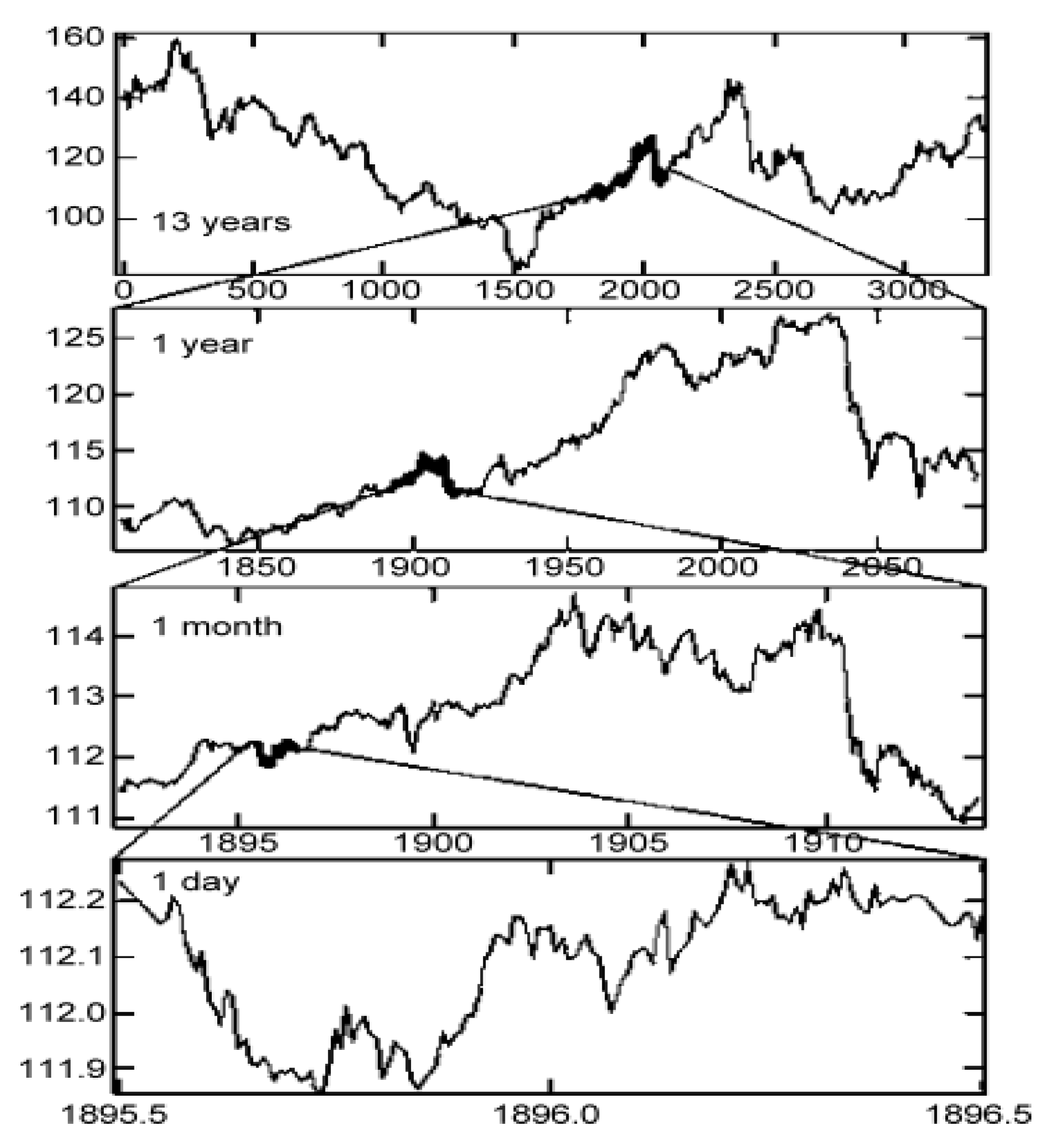
Figure 6.
Weierstrass time series.
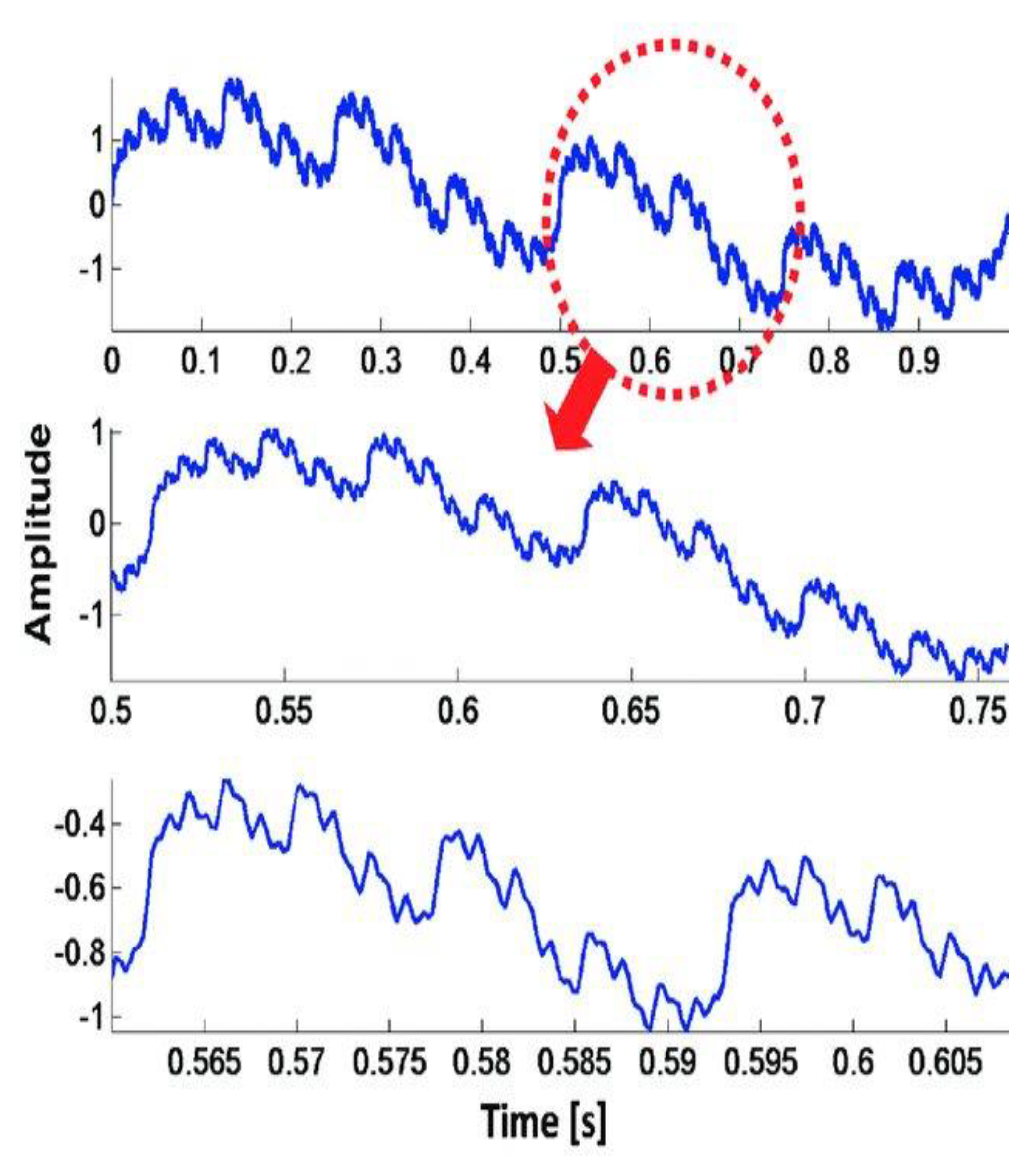
Figure 7.
A set of deterministic fractals[1,4] (a) Weierstrass function, (b) Sierpinski triangle, (c) Menger Sponge, (d) Recursive tree, (e) Barnsley fern.
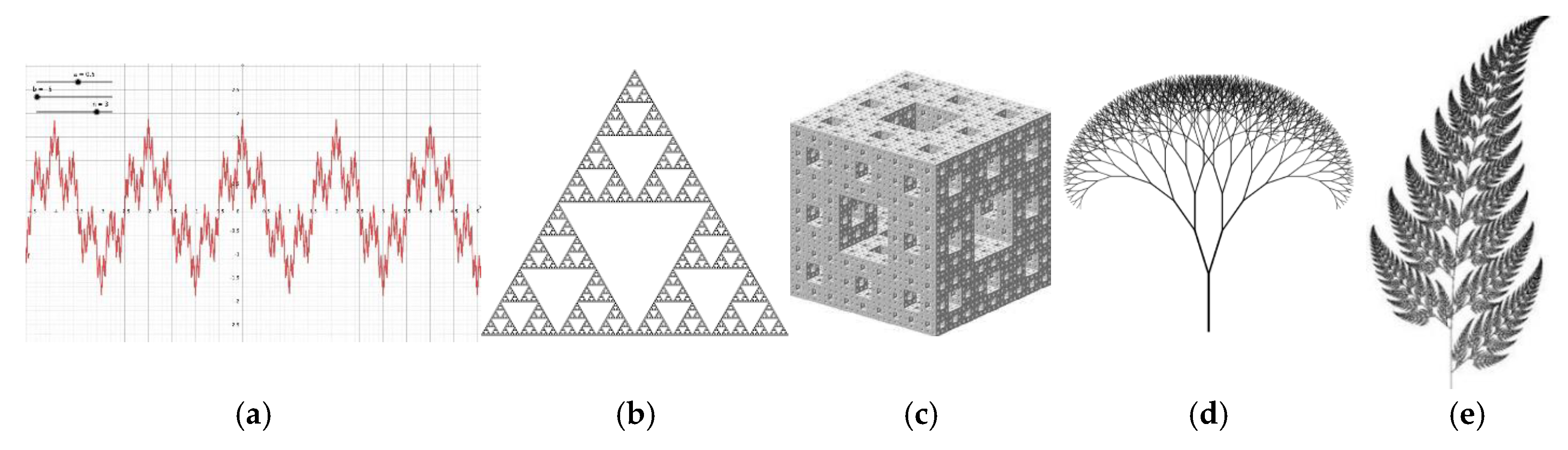
Figure 8.
A set of natural statistical fractals[2,5] (f) brain activity[7], (g) Coastline, (h) Tree branches1, (i) Natural Fern.
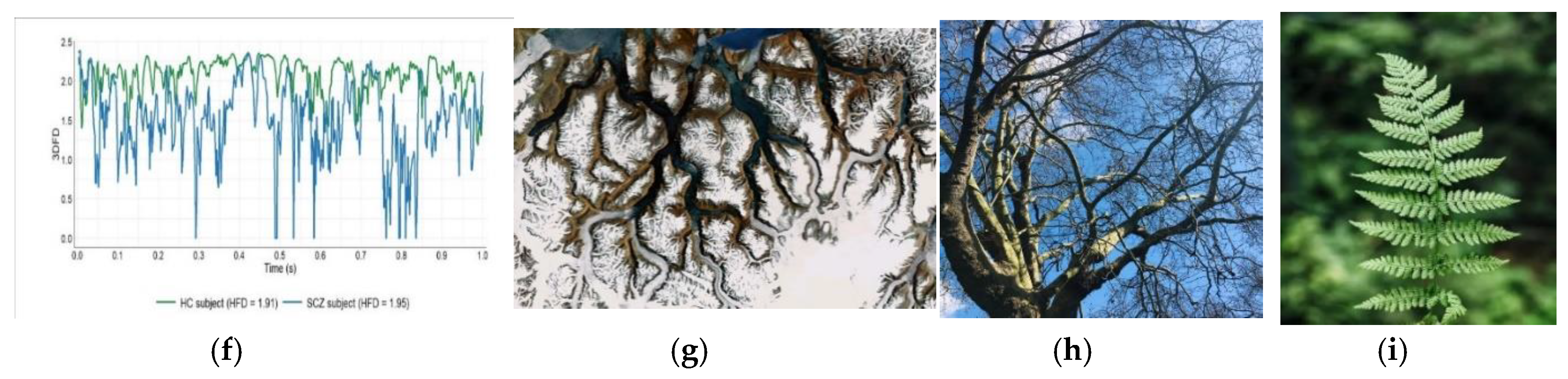
Figure 9.
Tree branches (Colin Drysdale).
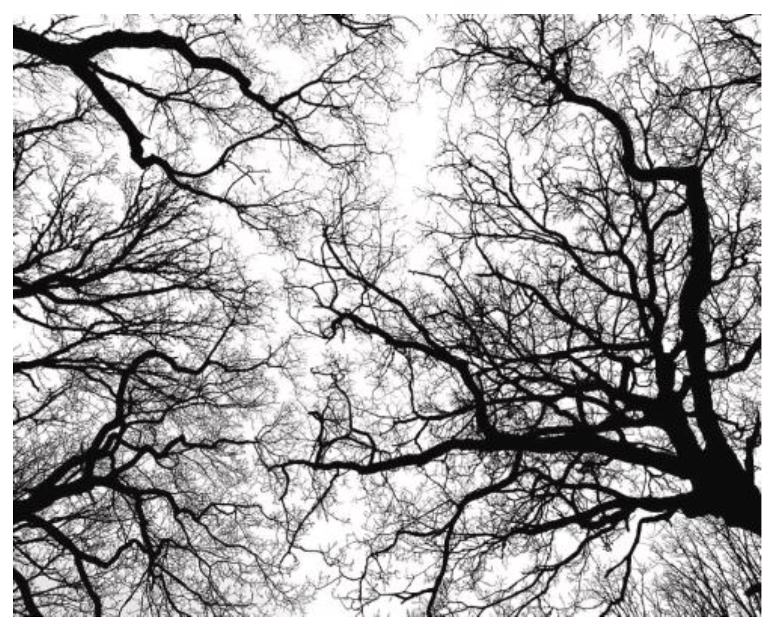
Figure 10.
Vascular system[9].
Figure 10.
Vascular system[9].
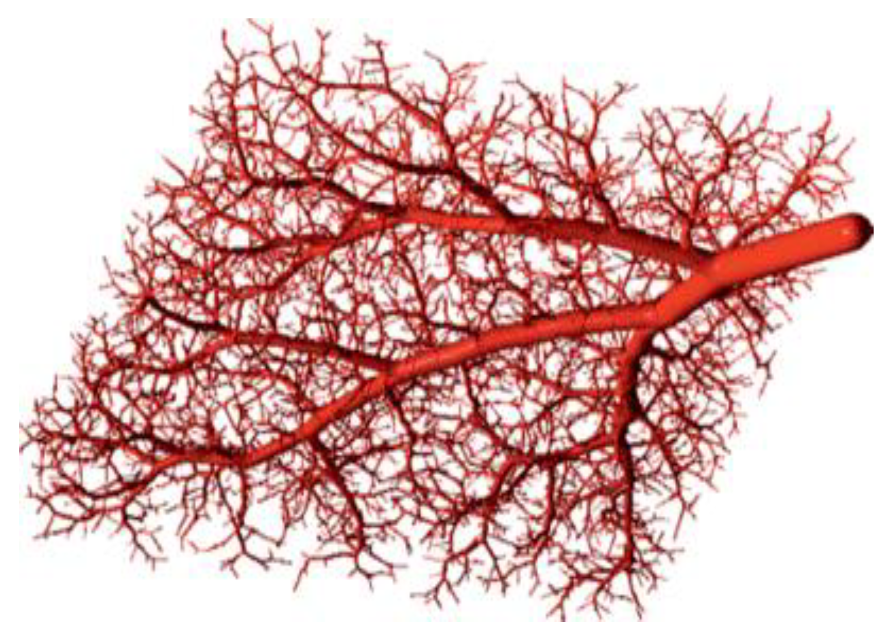
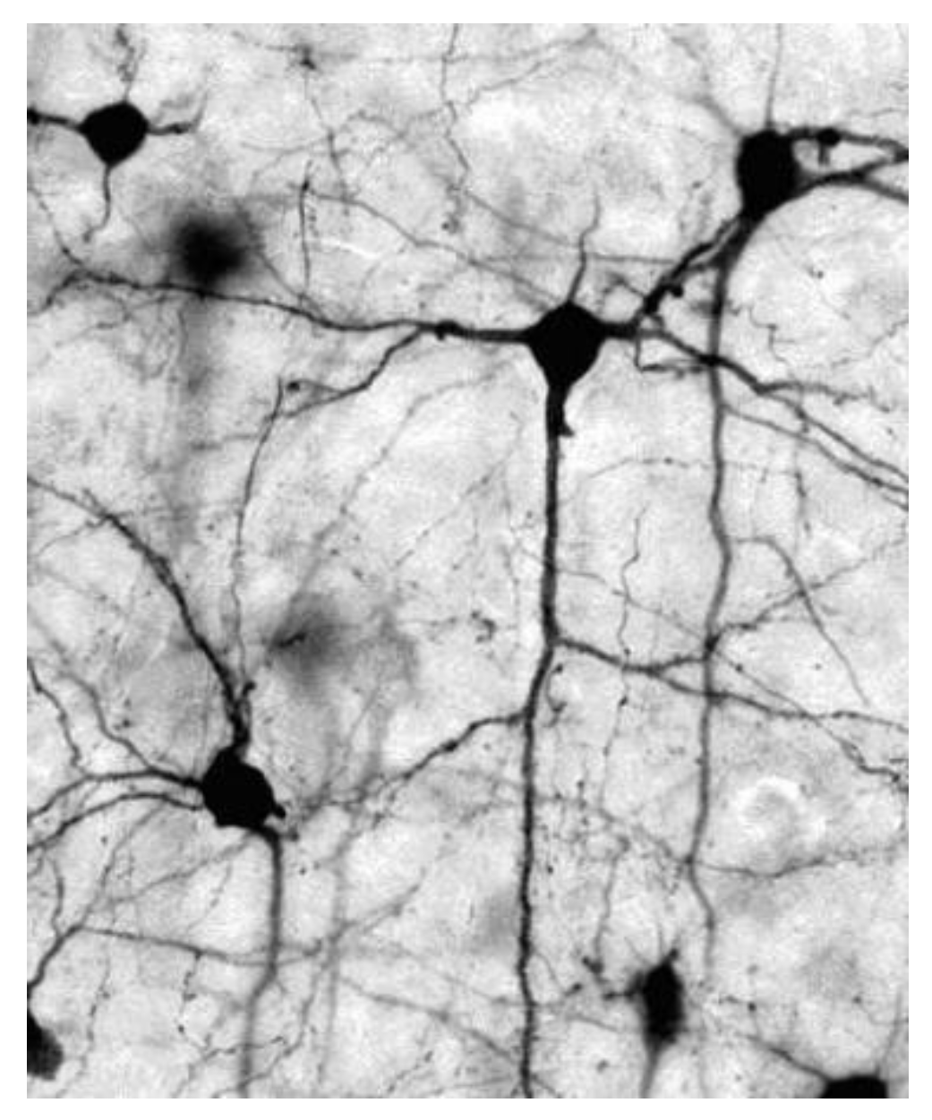
Figure 12.
Slime Mold[1].
Figure 12.
Slime Mold[1].
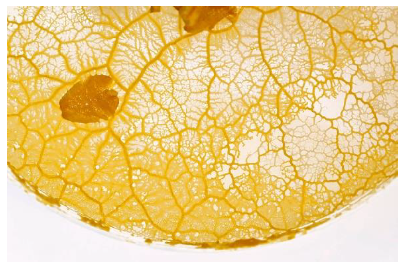
Figure 13.
Bacterial colony[11].
Figure 13.
Bacterial colony[11].
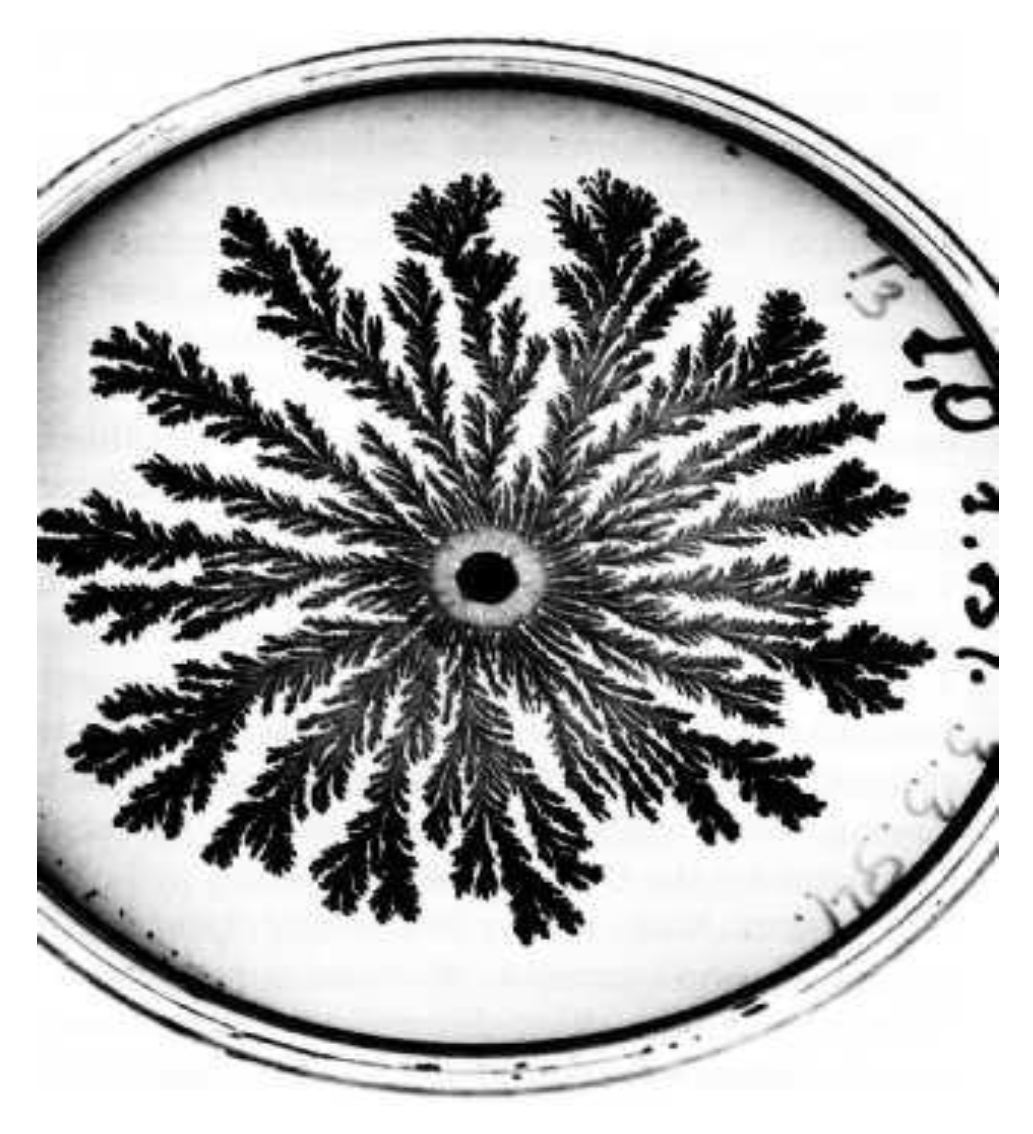
Figure 14.
Bioluminescence Algae (iStoke).
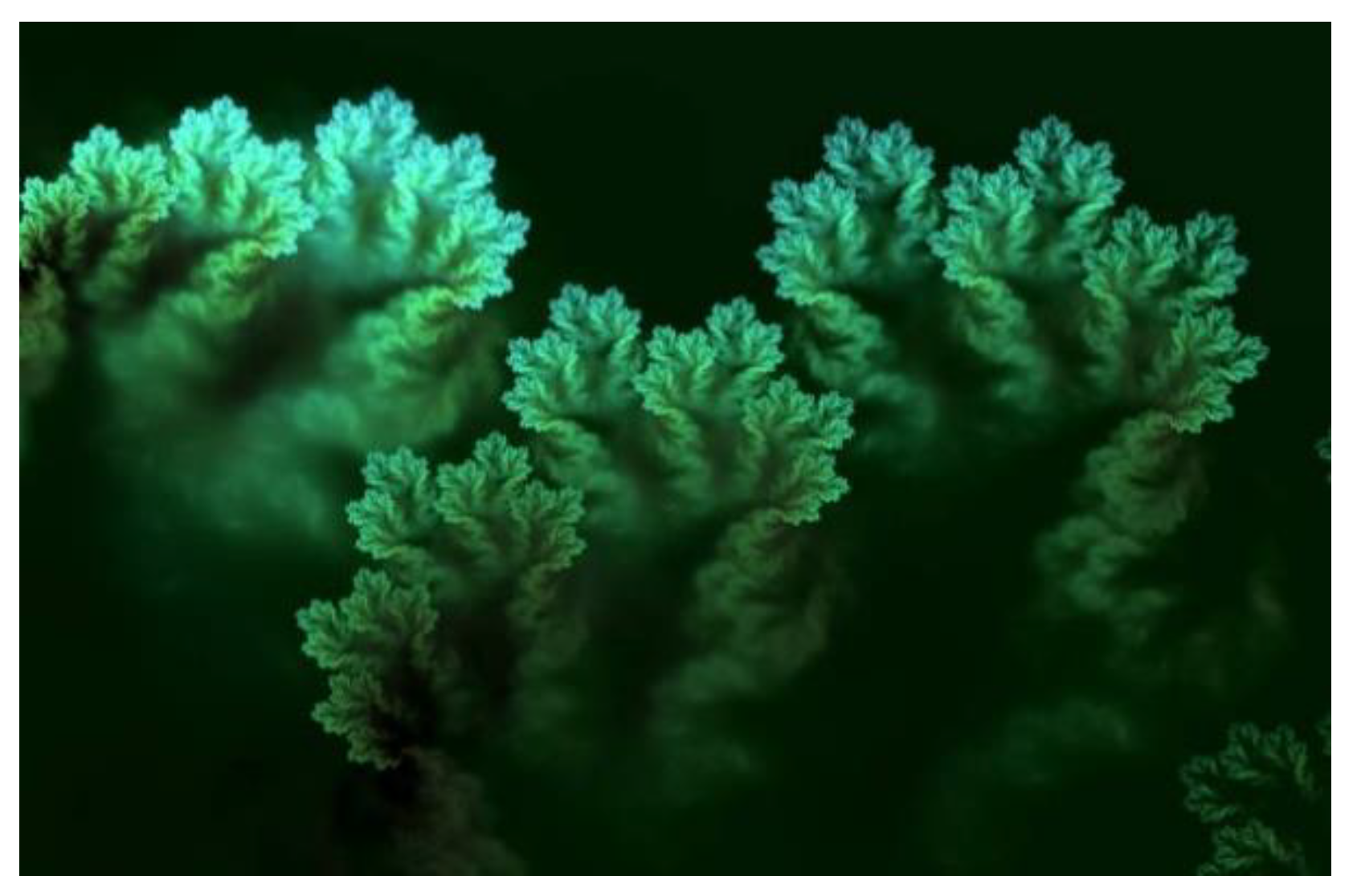
Figure 15.
Laniakea Supercluster (Sciences et Avenir).
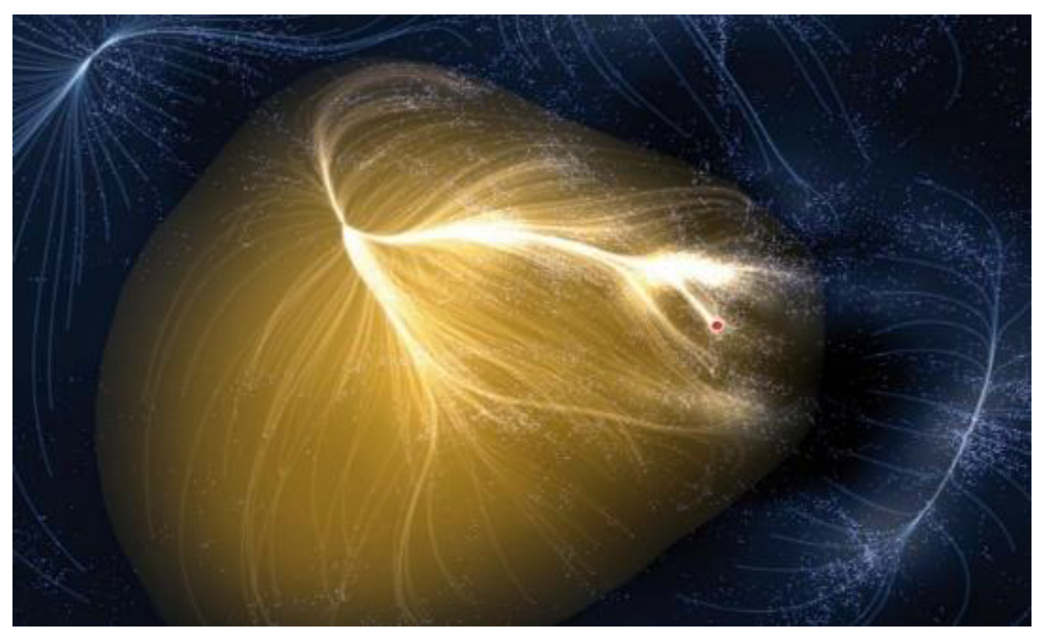
Figure 16.
Cosmic Web (Millennium run).
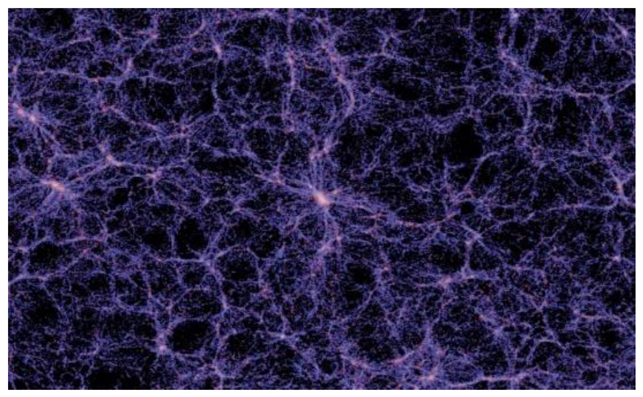
Figure 17.
Simulation of earthquake time series (52°North).
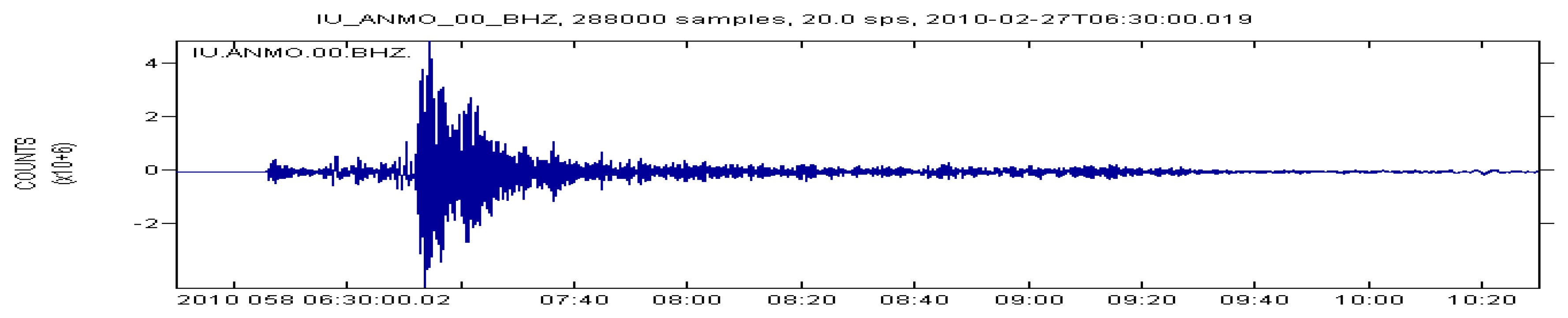
Figure 20.
Different Fractal Antenna Designs (j) Monopole-type Sierpinski design[24],(k) Menger sponge design[24],(l) biosensor hybrid design[32].
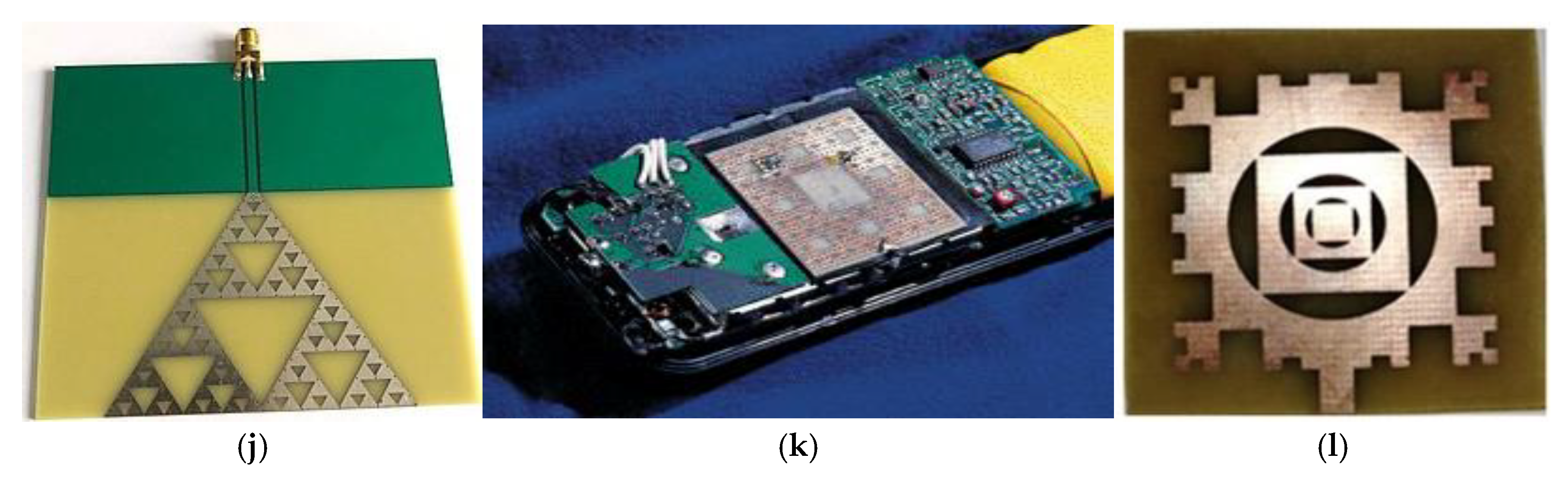
Figure 22.
turbulence with three iterations[34].
Figure 22.
turbulence with three iterations[34].
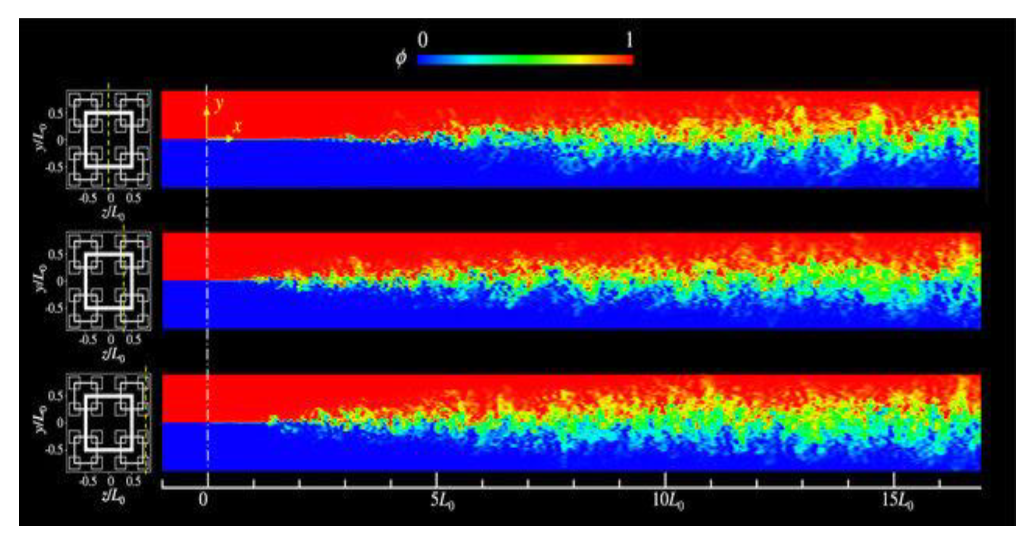
Figure 23.
Medium Disturbance density[34].
Figure 23.
Medium Disturbance density[34].
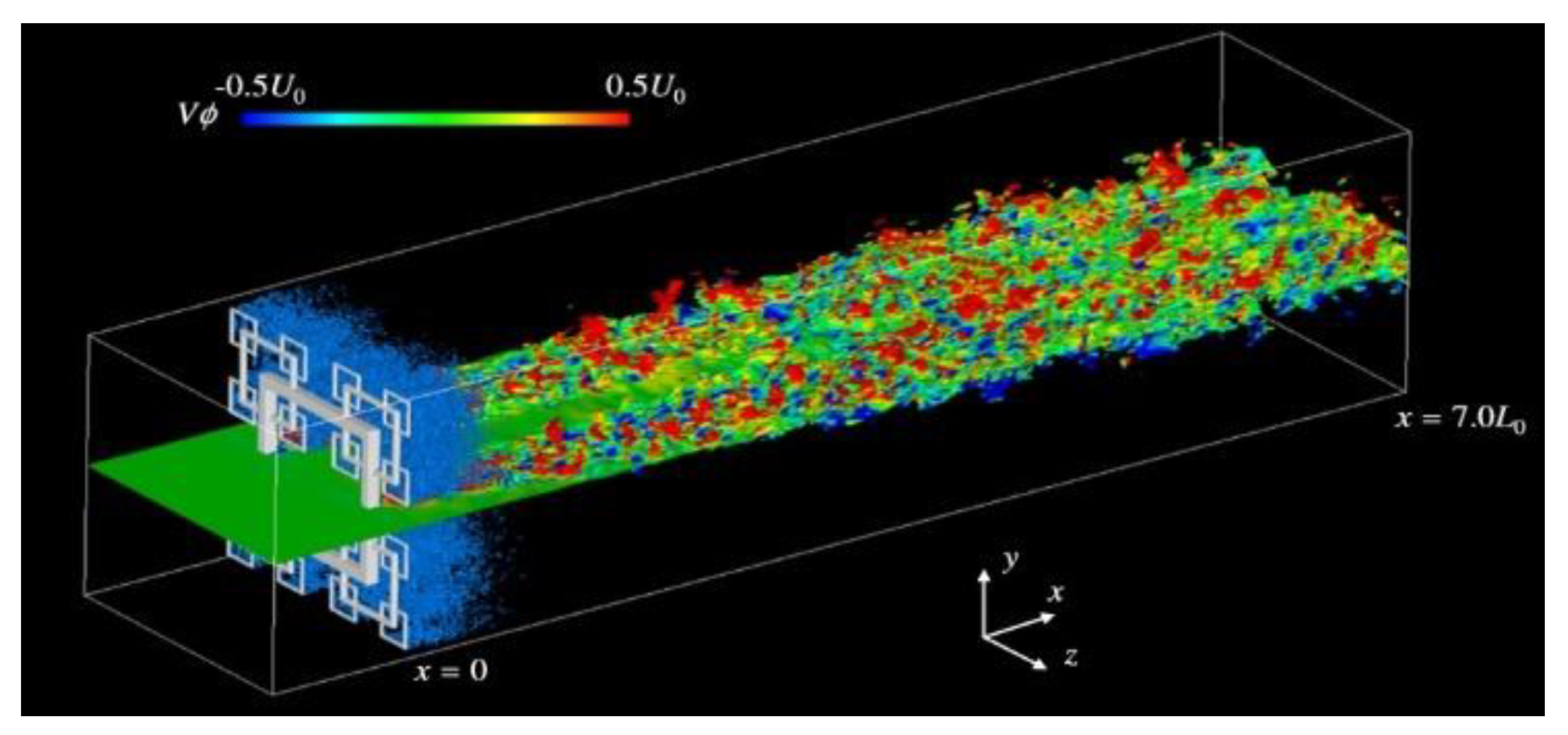
Figure 24.
Plasmonic fractal design of Ag layer.
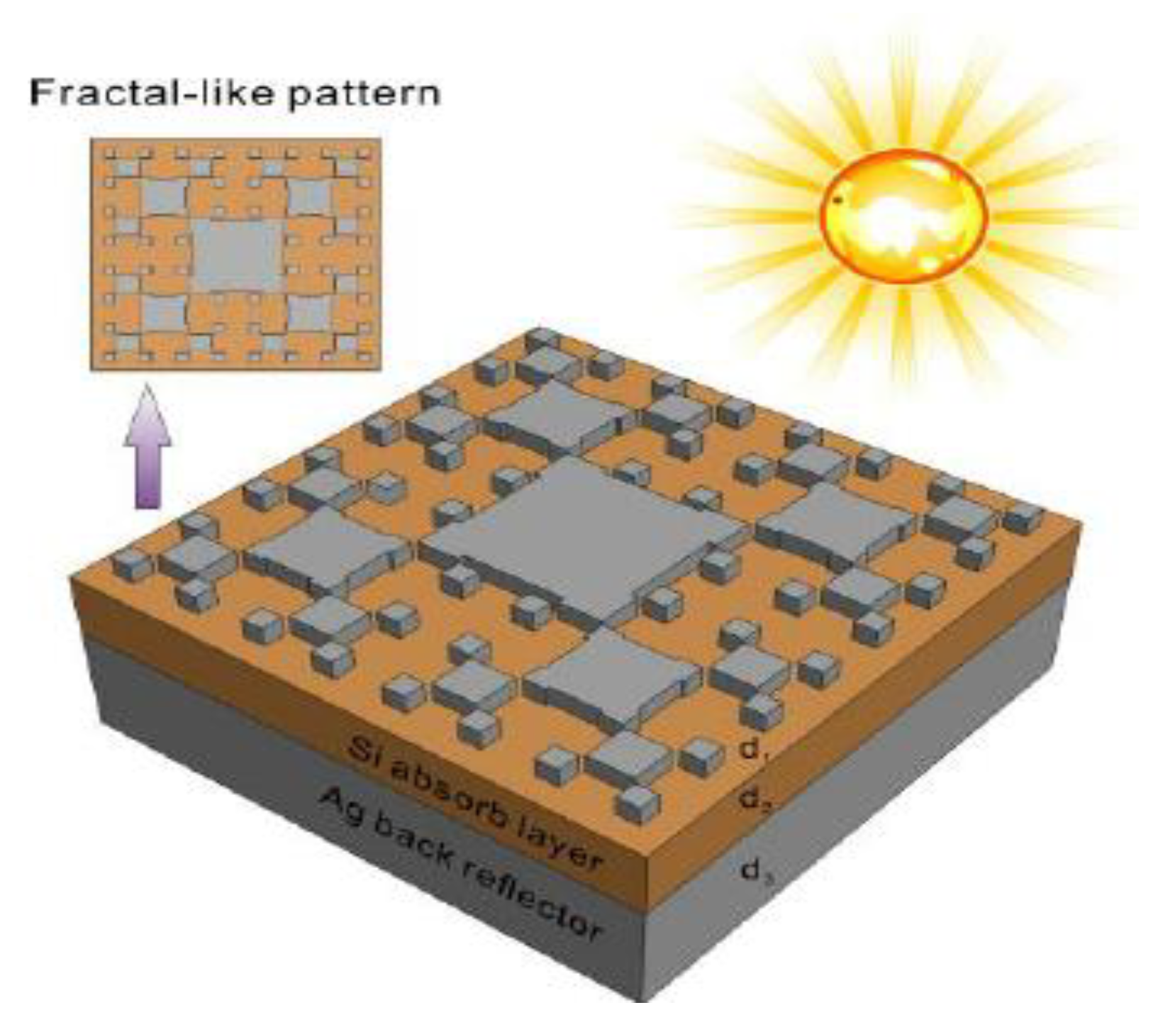
Figure 25.
Quantum efficiencies of different Ag layer designs.
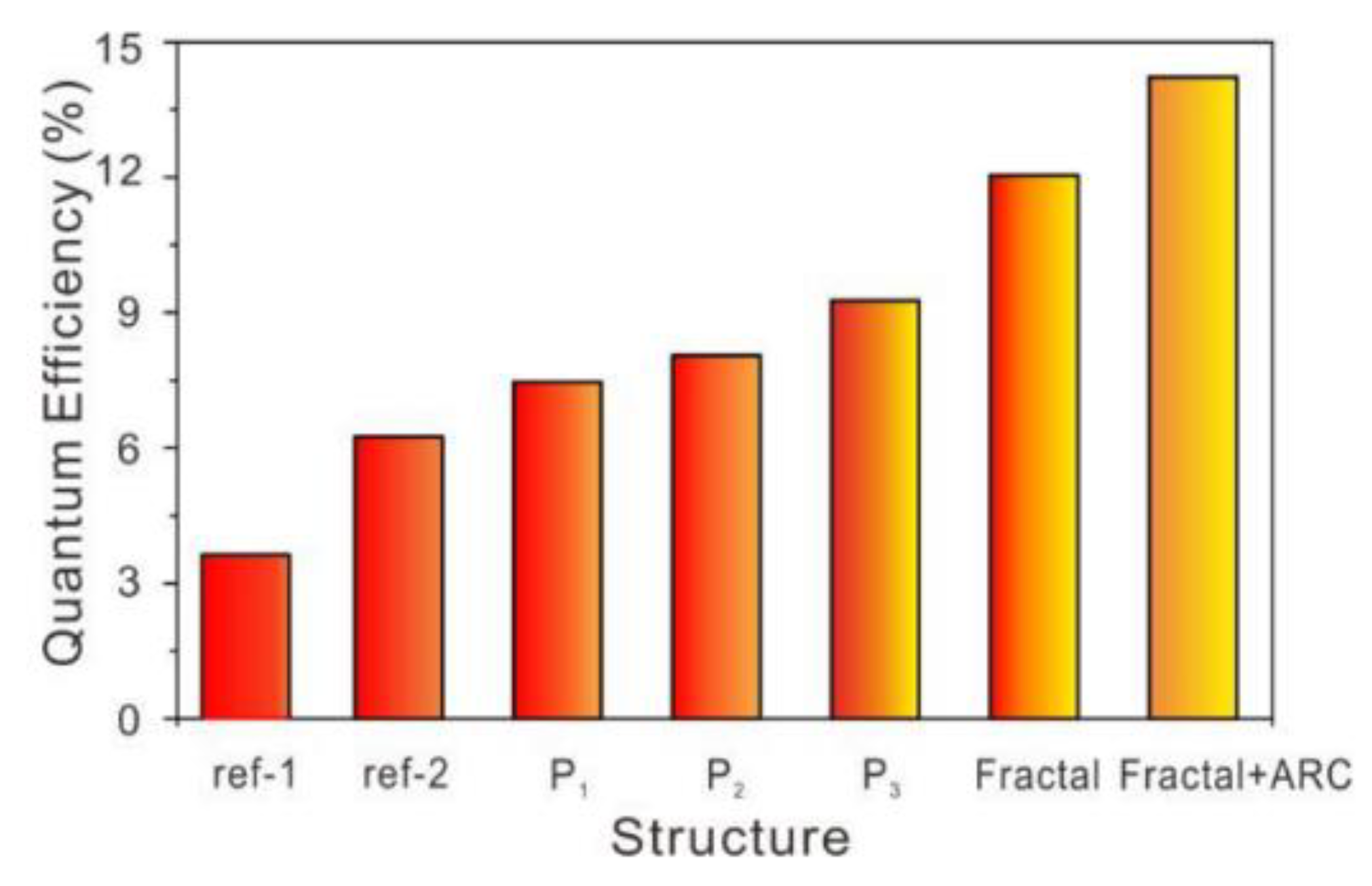
Figure 26.
Georg Christoph Lichtenberg.
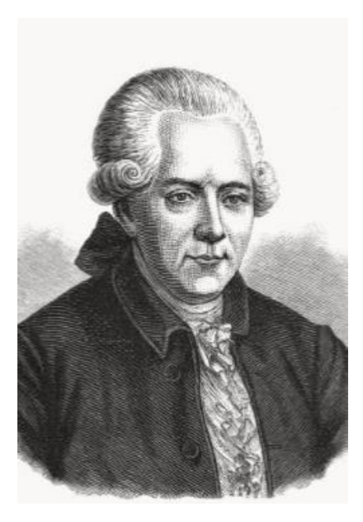
Figure 27.
Lichtenberg figures.
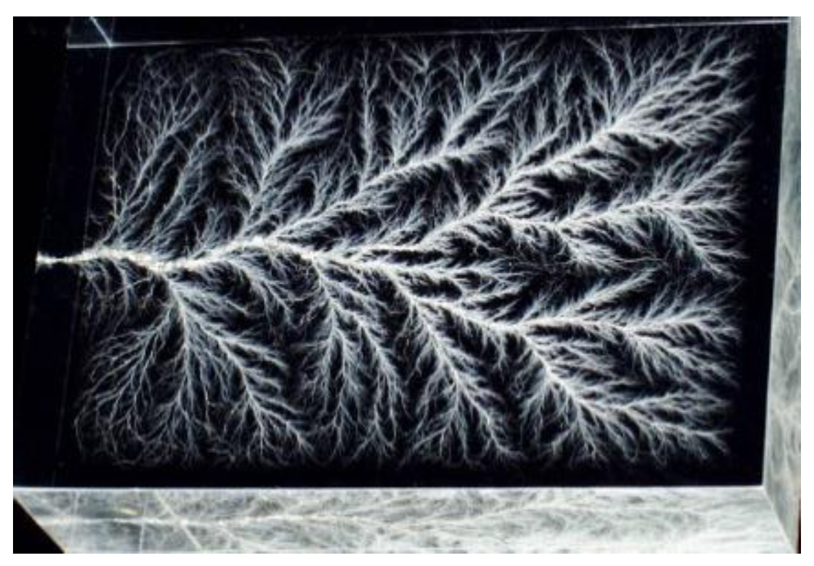
Figure 28.
Karl Weierstrass.
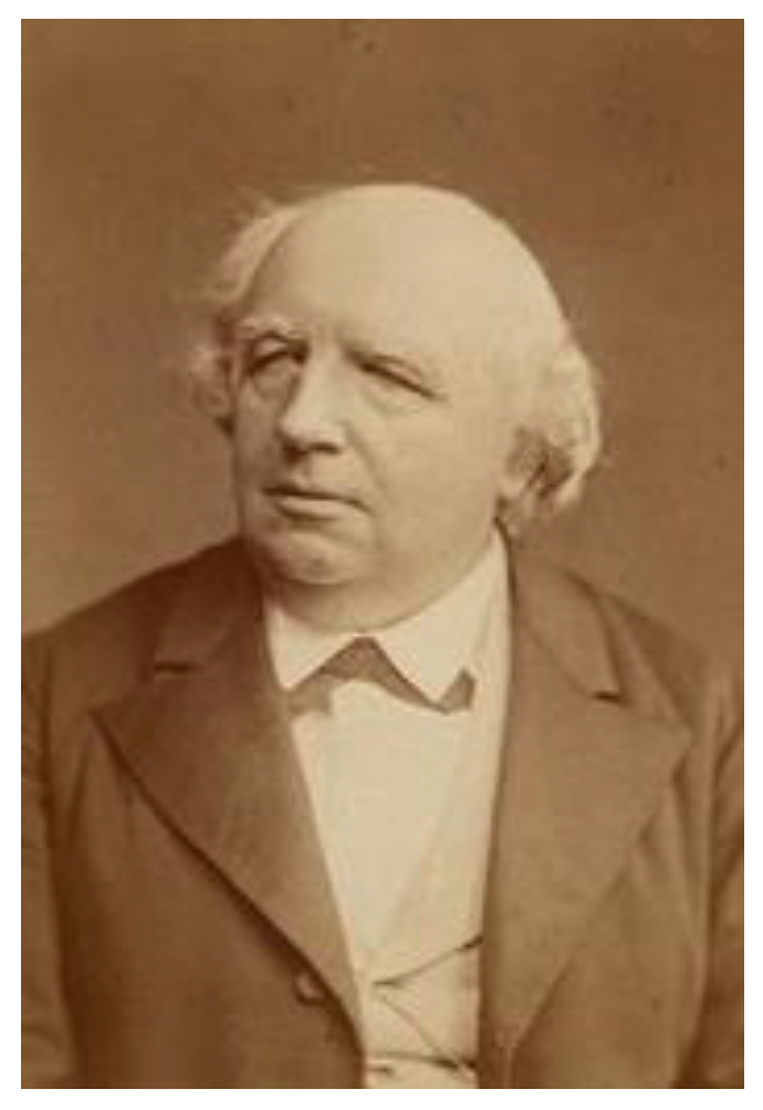
Figure 29.
Weierstrass function.
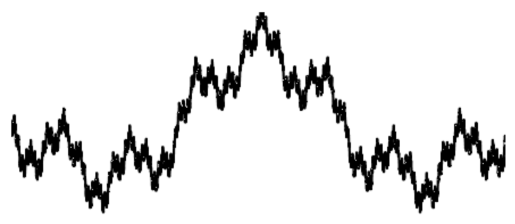
Figure 30.
Georg Cantor.
Figure 31.
Cantor Set.
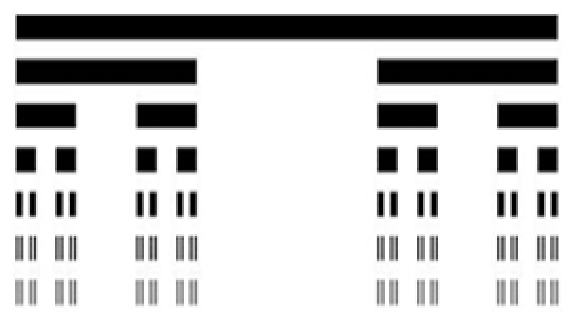
Figure 32.
Gaston Juilia.
Figure 33.
Juilia Set.
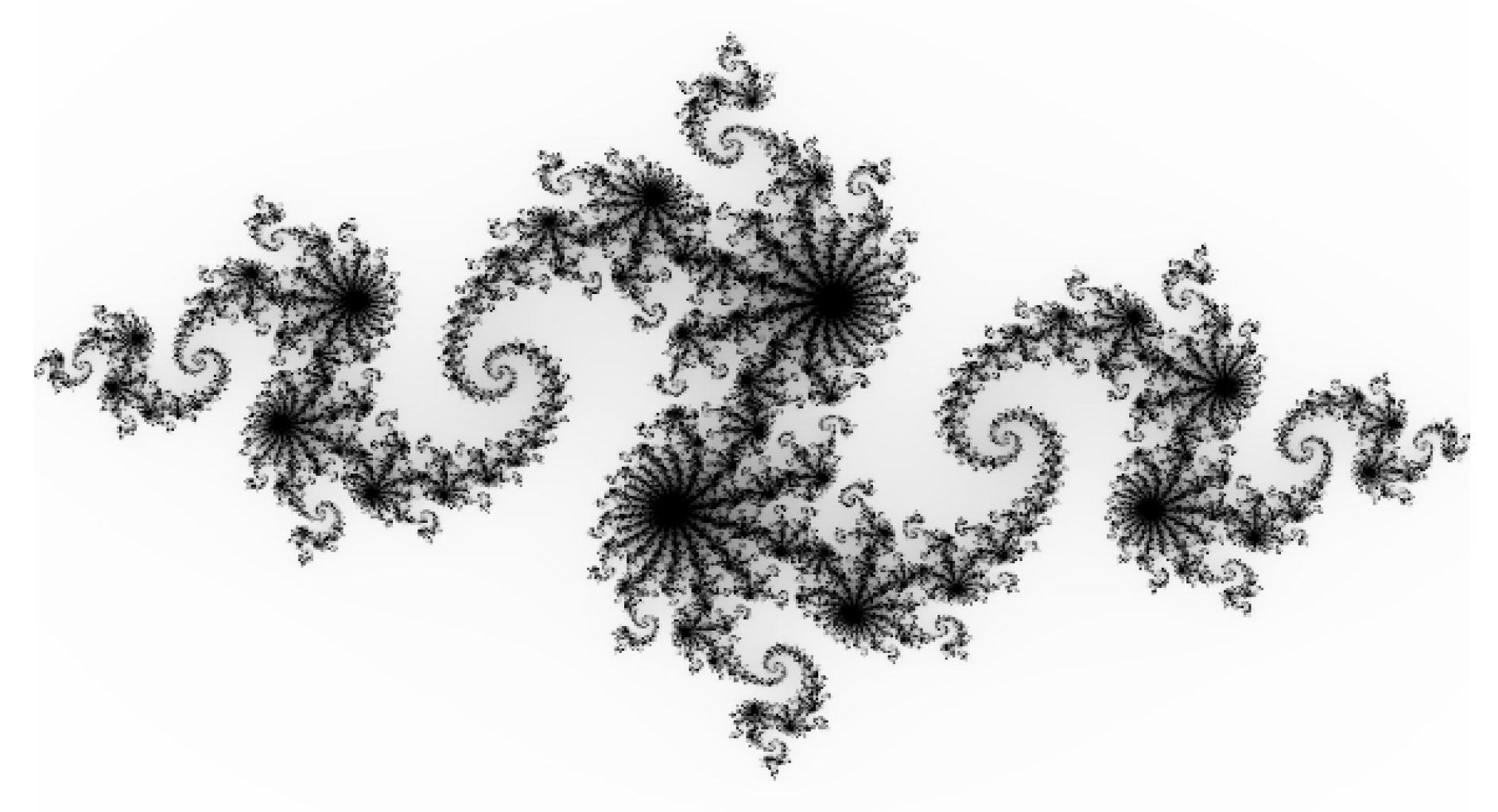
Figure 34.
Benoît Mandelbrot.
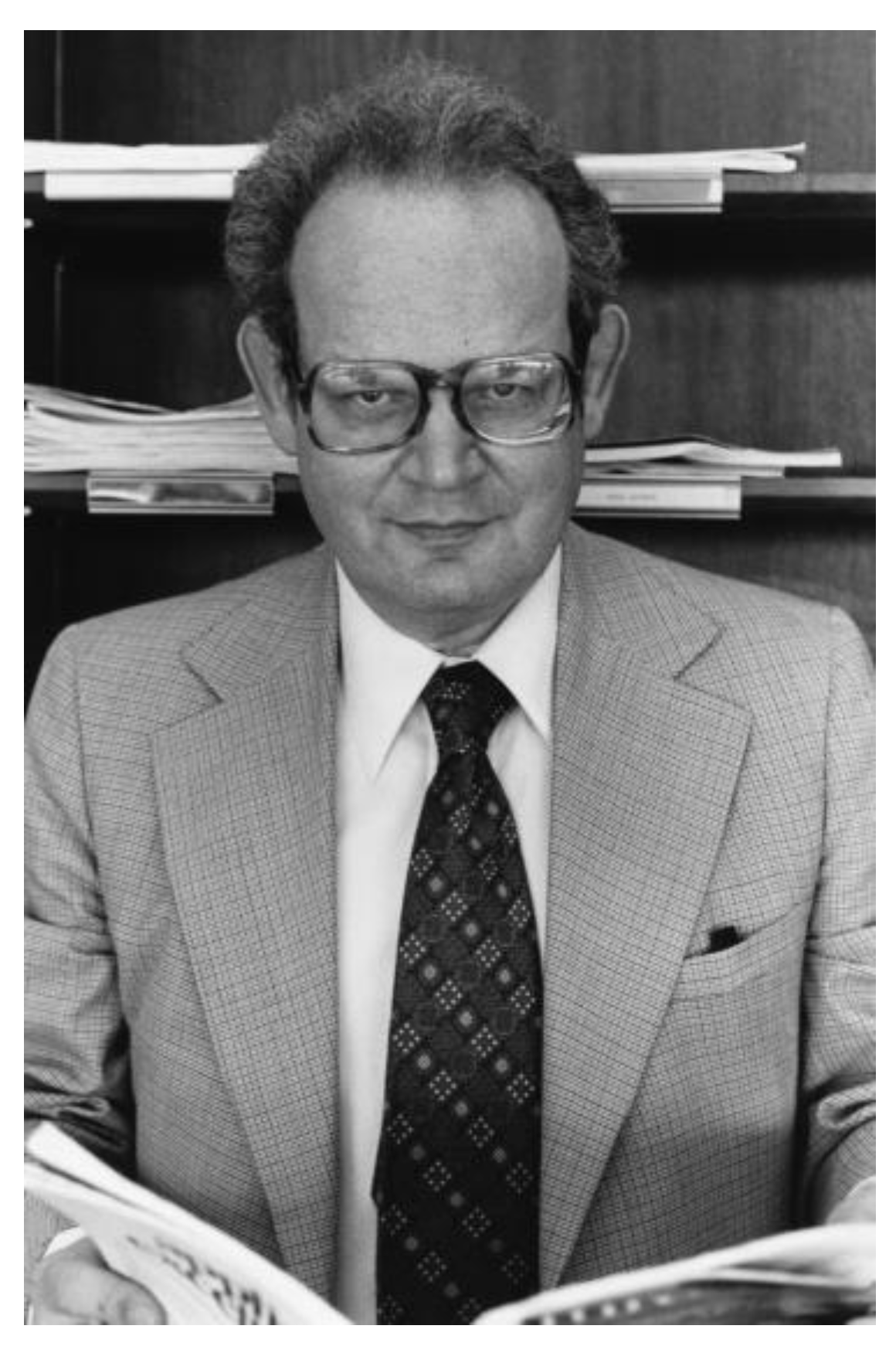
Figure 35.
Mandelbrot set.
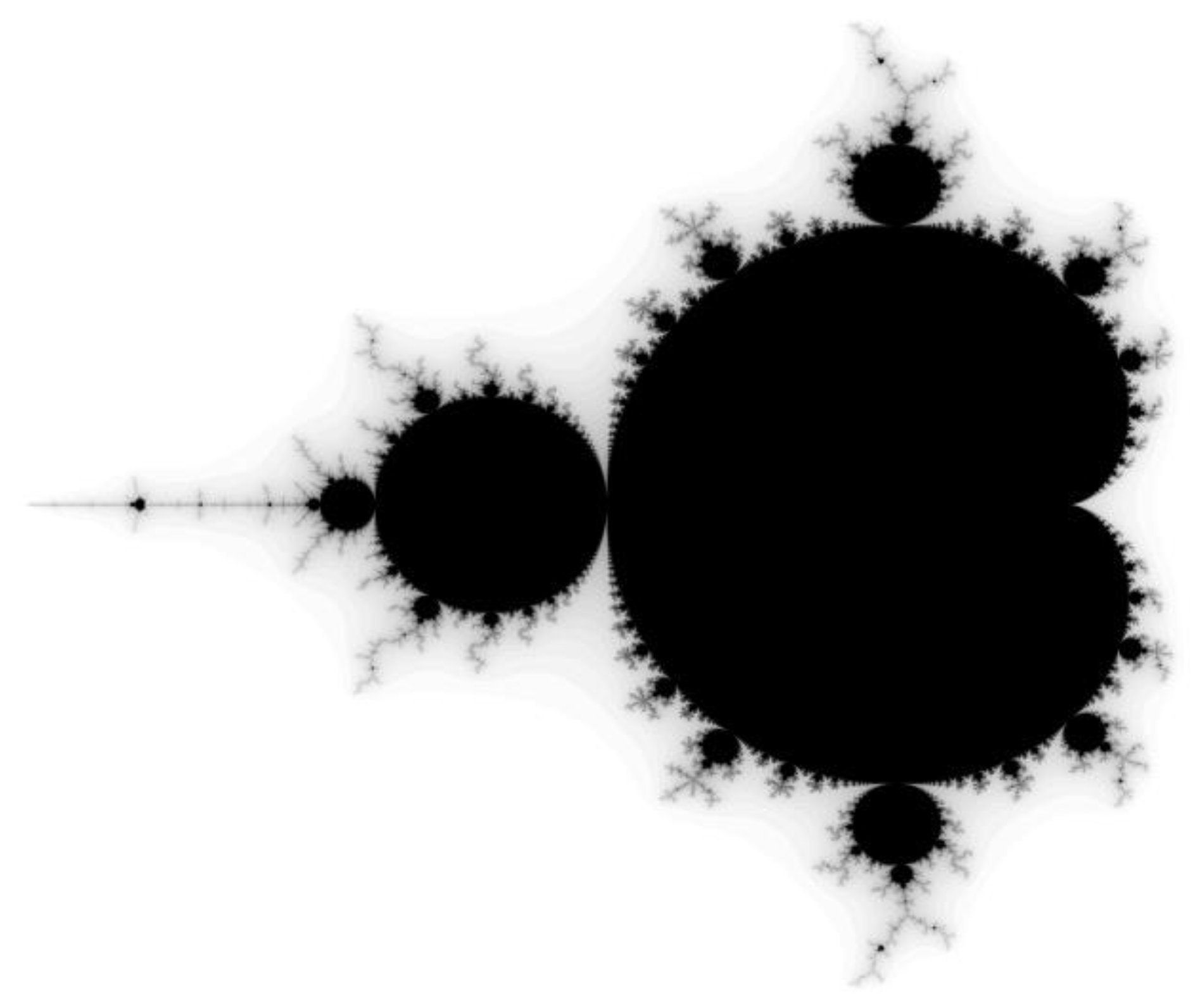
Figure 36.
Koch.
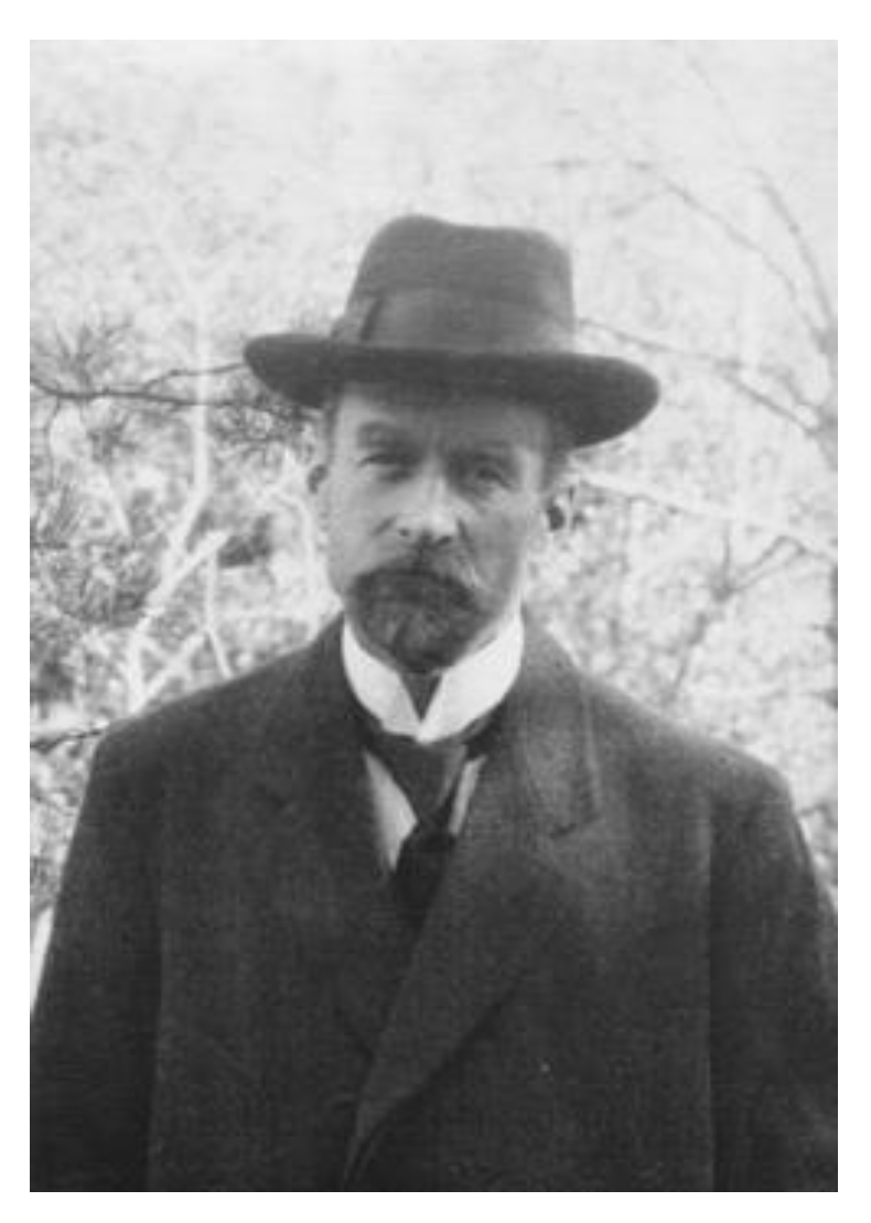
Figure 37.
Koch Snowflake.
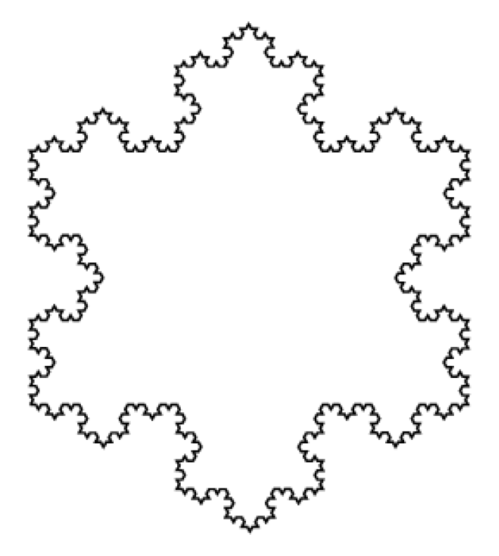
Figure 38.
Sierpiński.
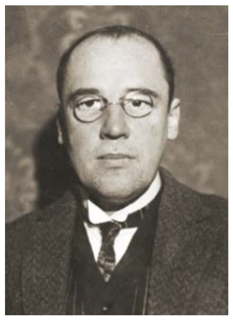
Figure 39.
Sierpiński triangle.
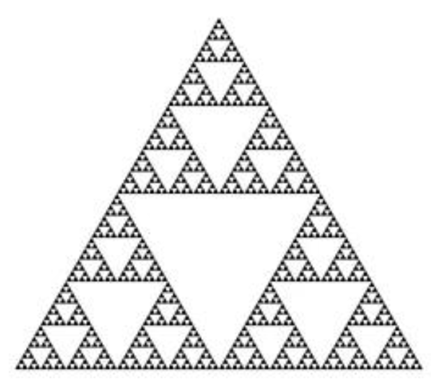
Figure 40.
Lévy.
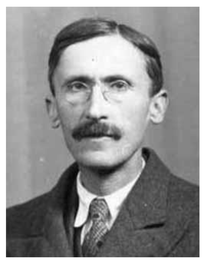
Figure 41.
Lévy C curve.
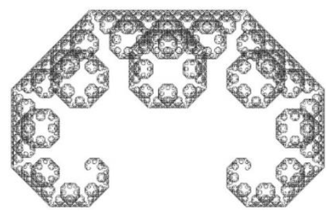
Figure 42.
Menger.
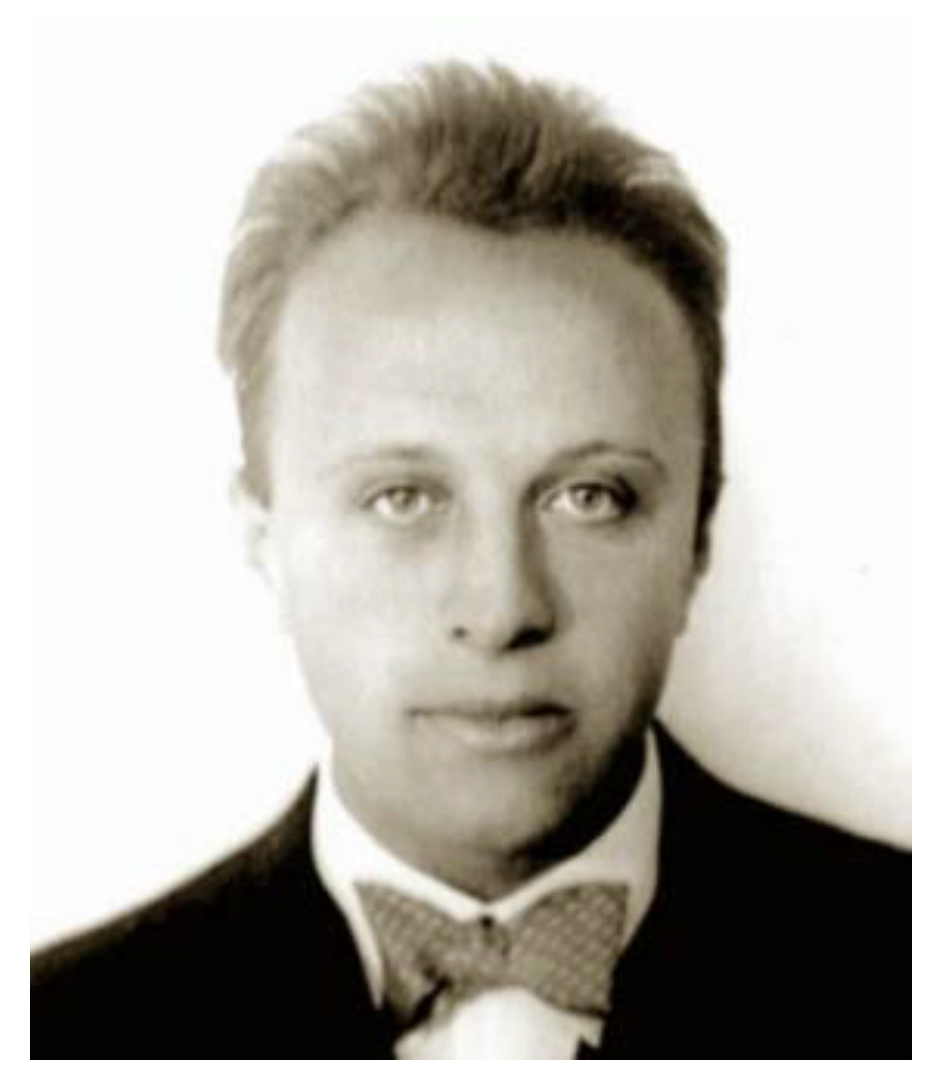
Figure 43.
Menger Sponge.
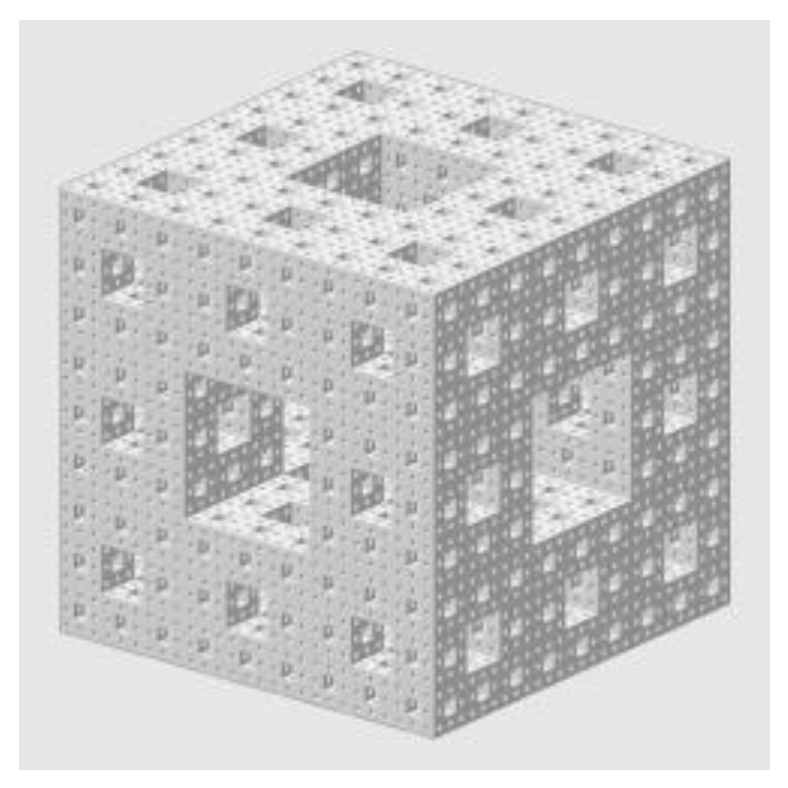
Figure 44.
Different Fractal orders with various dimensions.
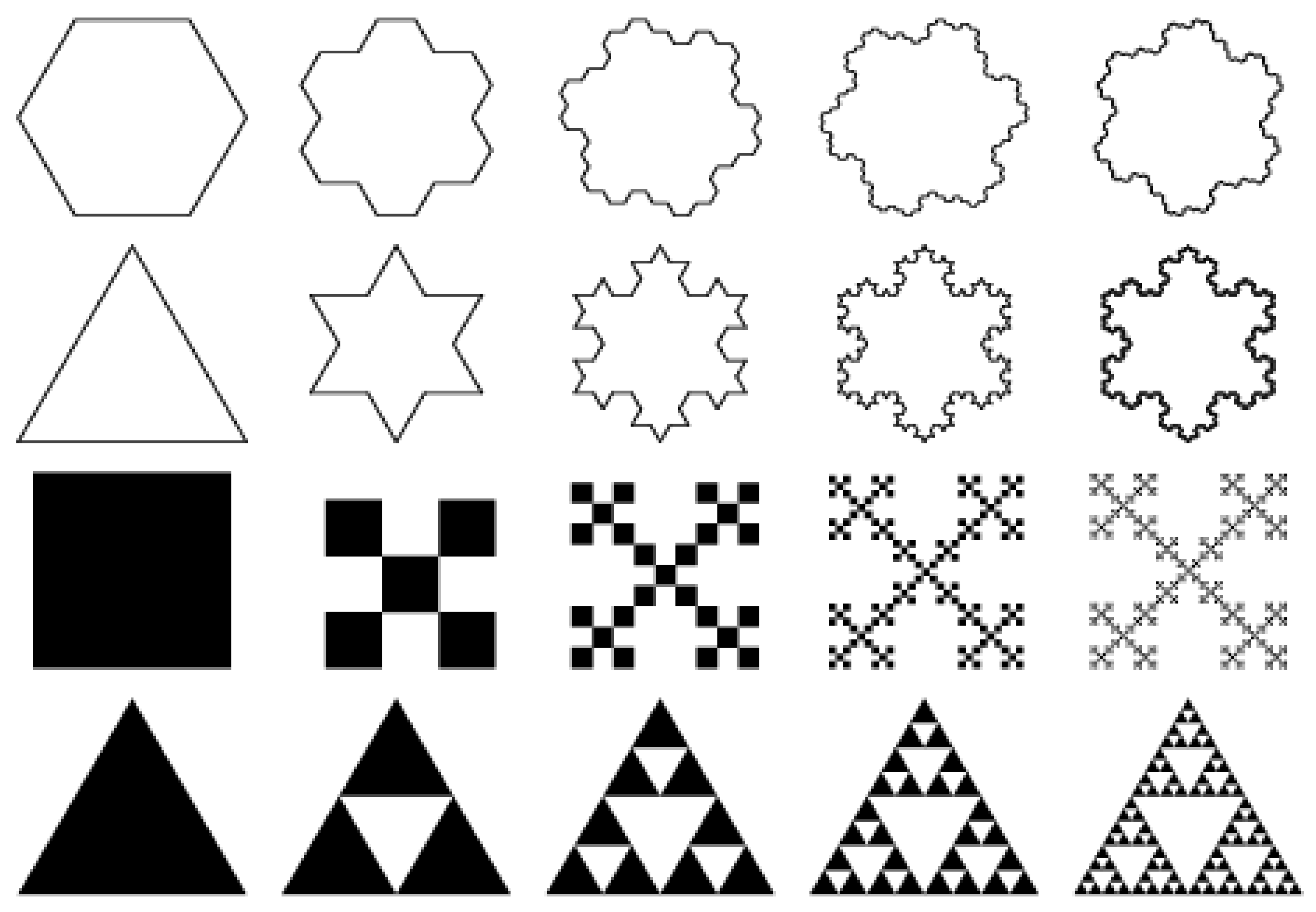
Figure 45.
Applied different box scales to determine the fractal dimension of Britain coastline.
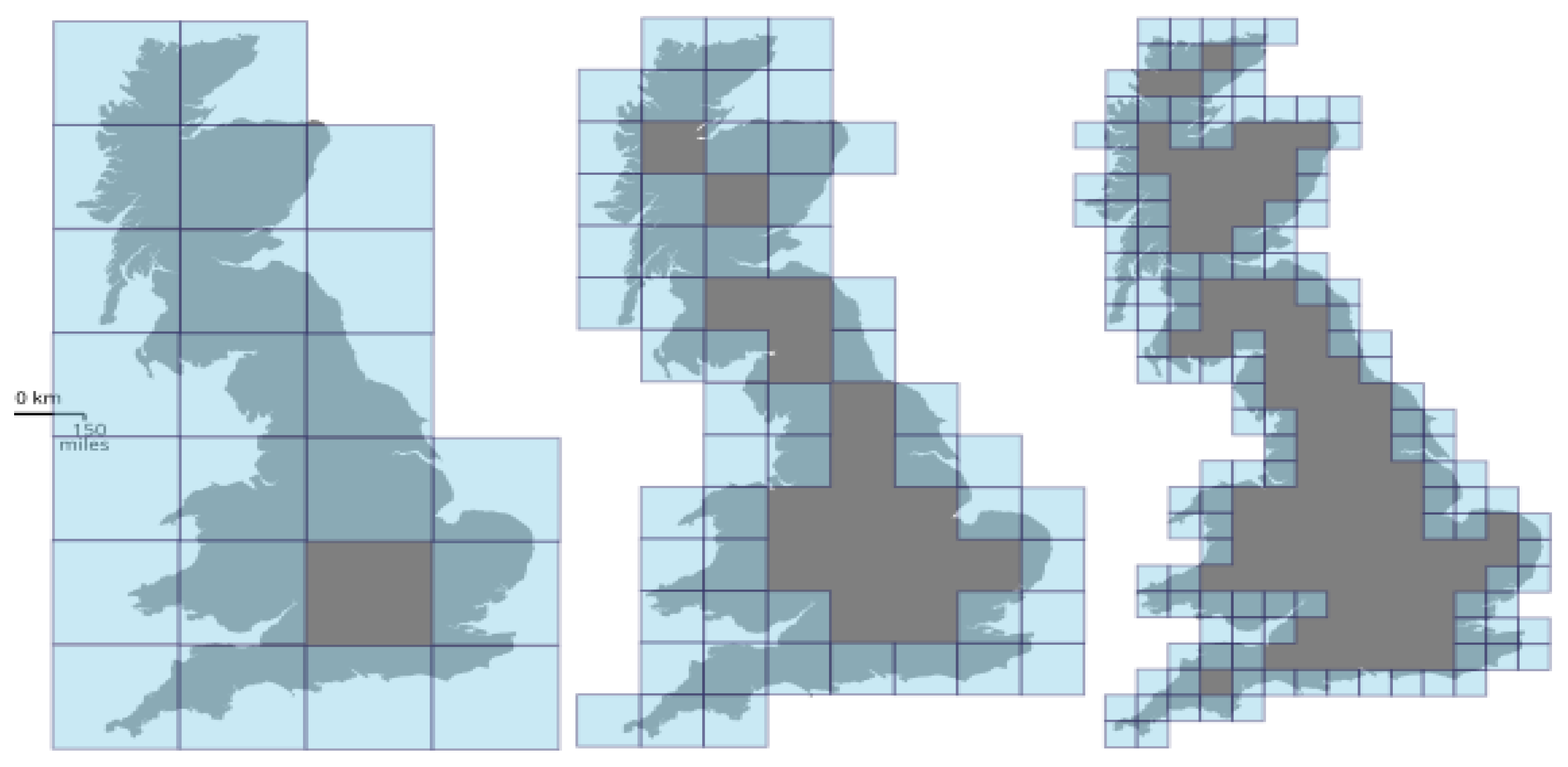
Figure 46.
Using fractal analysis determine the state of the biological system through fractal dimension.
Figure 46.
Using fractal analysis determine the state of the biological system through fractal dimension.
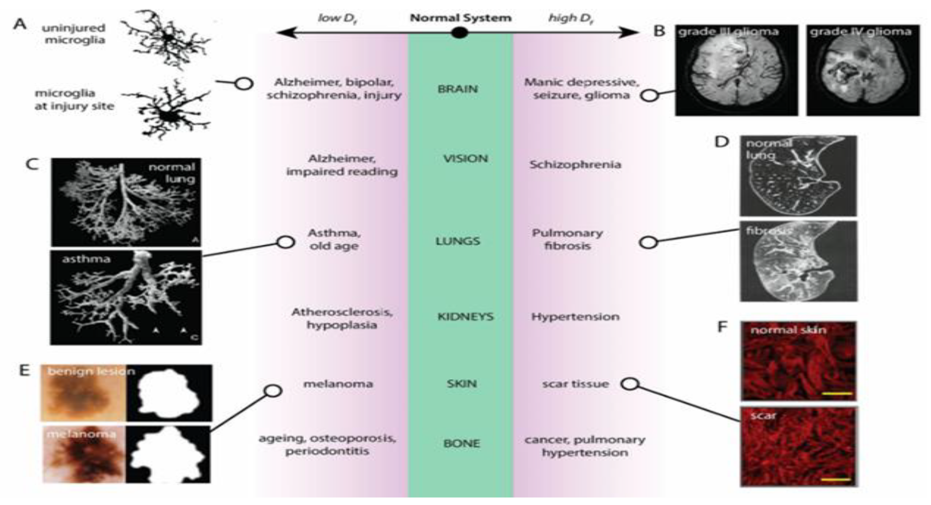
Figure 47.
Chromatin 3D fractal globule Model.
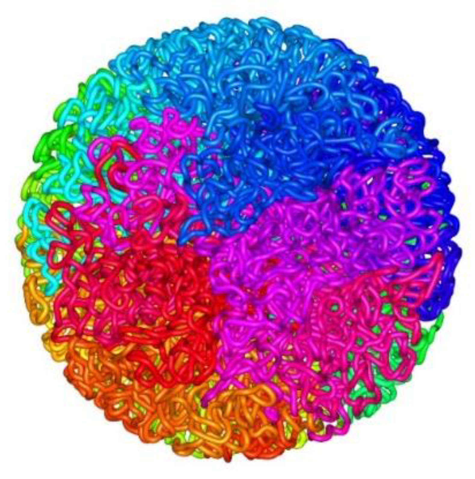
Figure 48.
An increase of fractal dimension by chromatin heterogeneity.
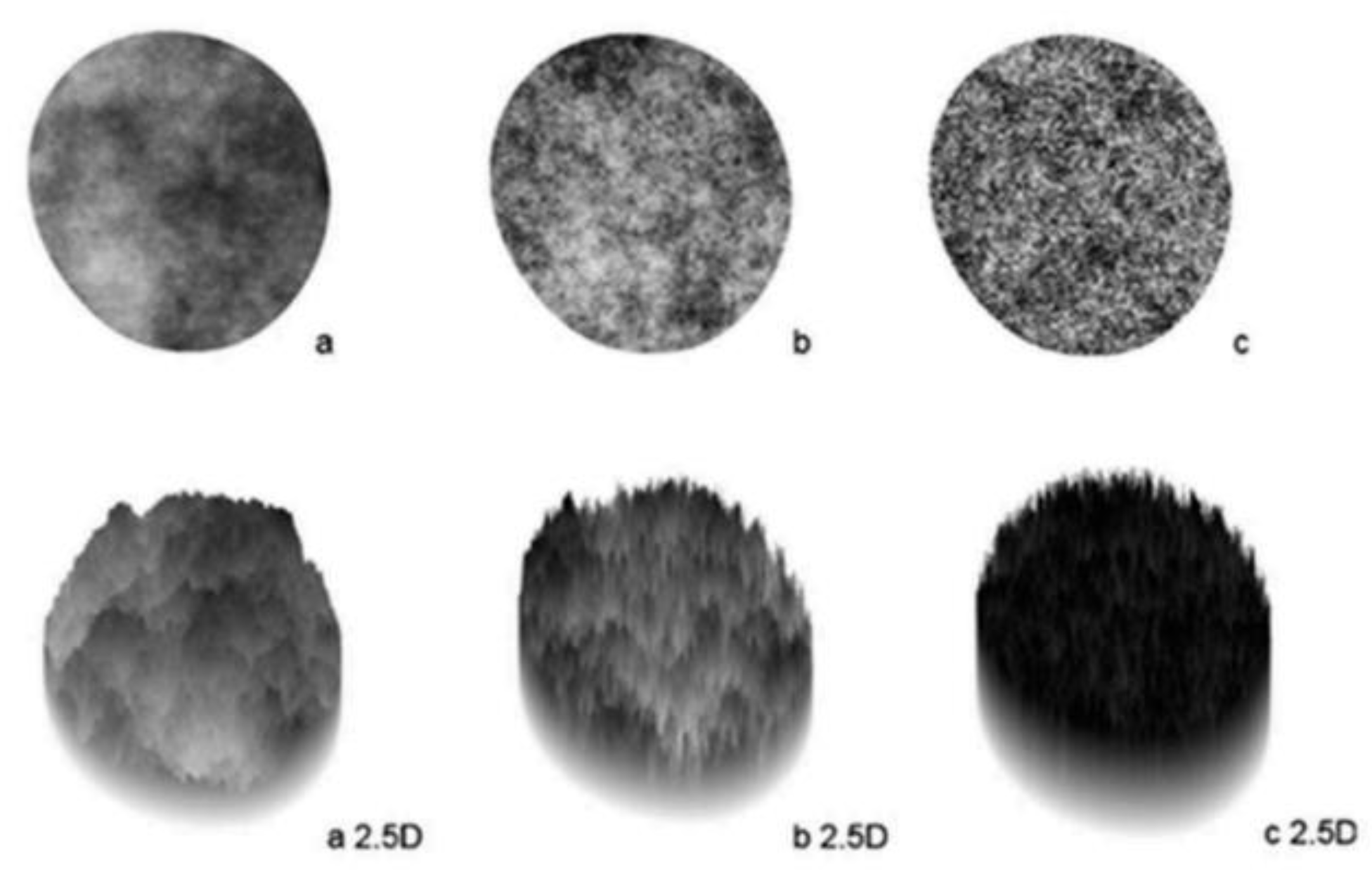
Figure 49.
Different D of normal, immortal, and cancer cells.
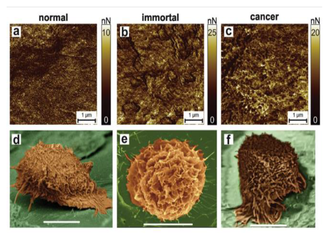
Figure 50.
Higher Fractal dimension shows more ability[49].
Figure 50.
Higher Fractal dimension shows more ability[49].
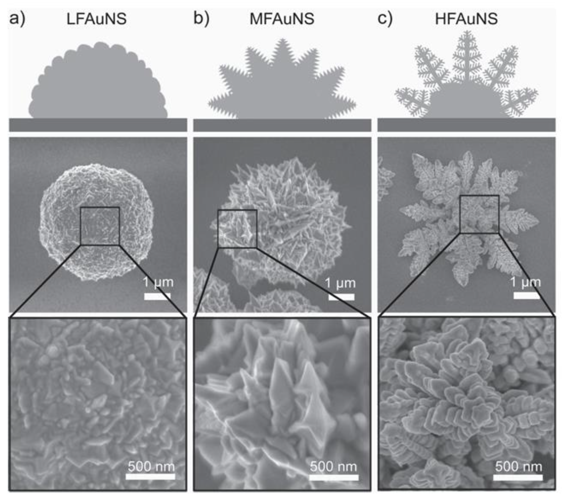
Figure 51.
The temporal growth of clusters with a fractal structure.
Figure 52.
Fractal structure of different organs (a) Coronary Arteries, (b) Lung Branches, (c) Renal Arteries, (d) Cerebellum MR image.
Figure 52.
Fractal structure of different organs (a) Coronary Arteries, (b) Lung Branches, (c) Renal Arteries, (d) Cerebellum MR image.
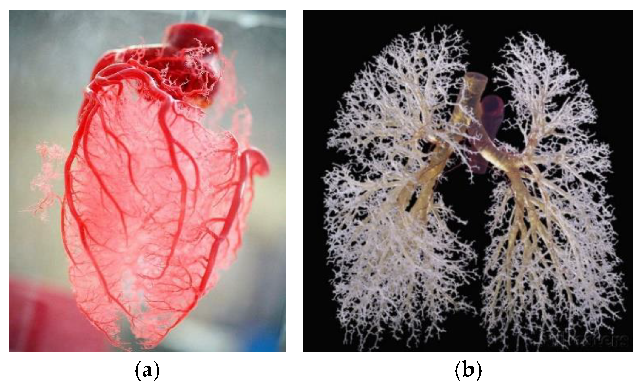
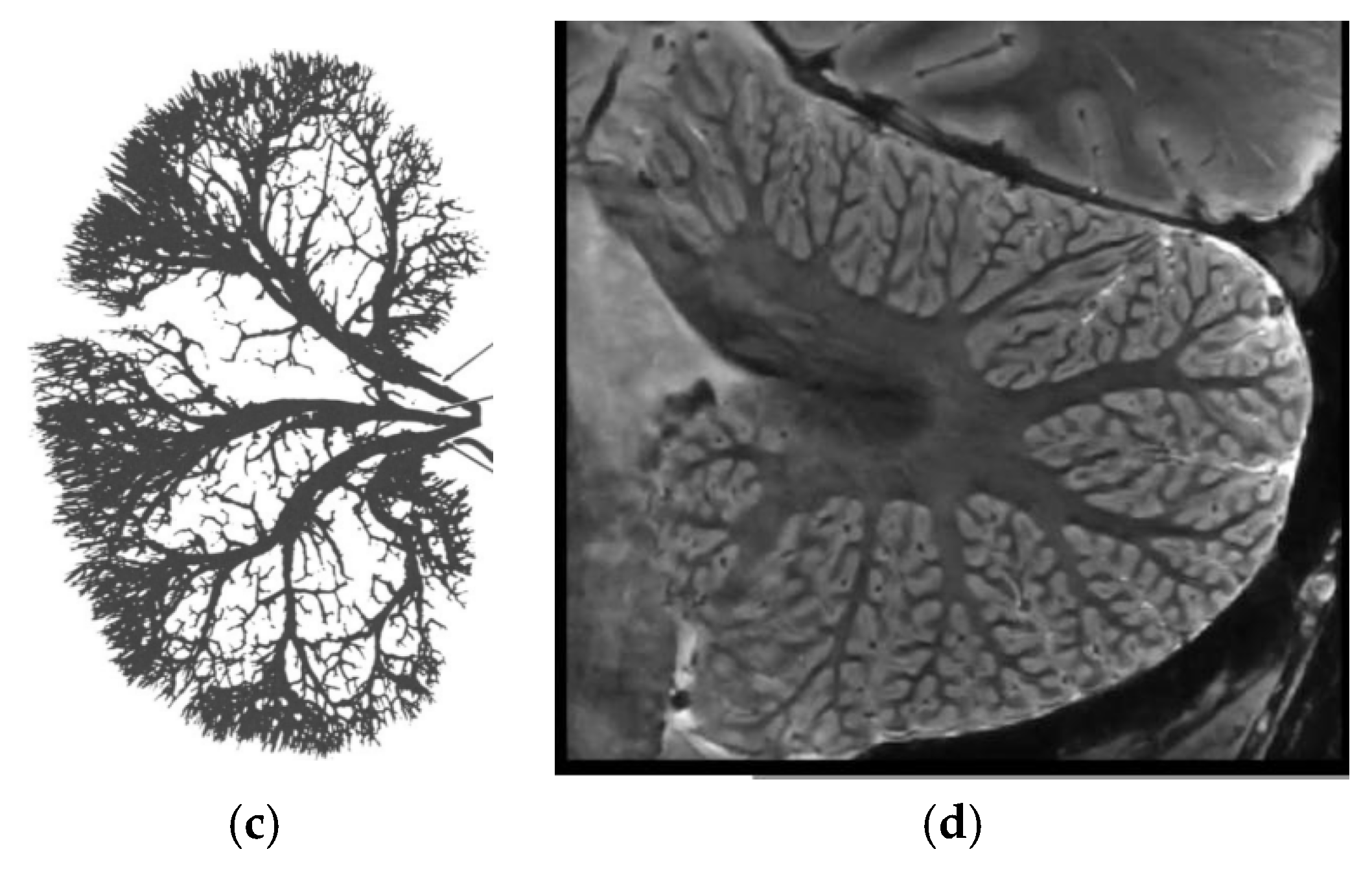
Figure 53.
MRI of benign and atypical meningiomas.
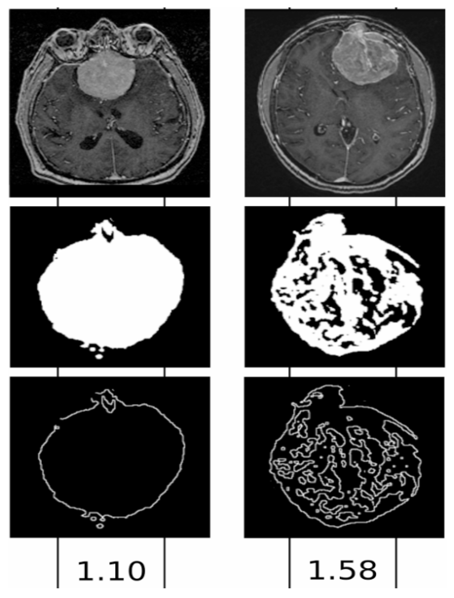
Figure 54.
Low and high cortical brain complexity.
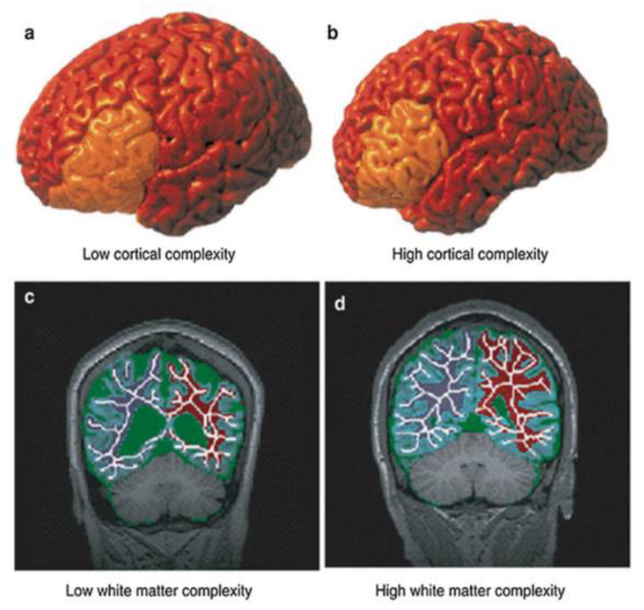
Figure 55.
Scale-invariant showing in heart rate behavior.
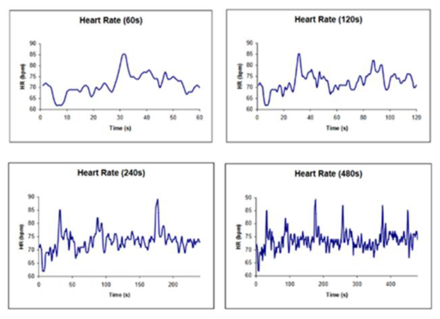
Figure 56.
Comparing HFD value of healthy and schizophrenia cases.
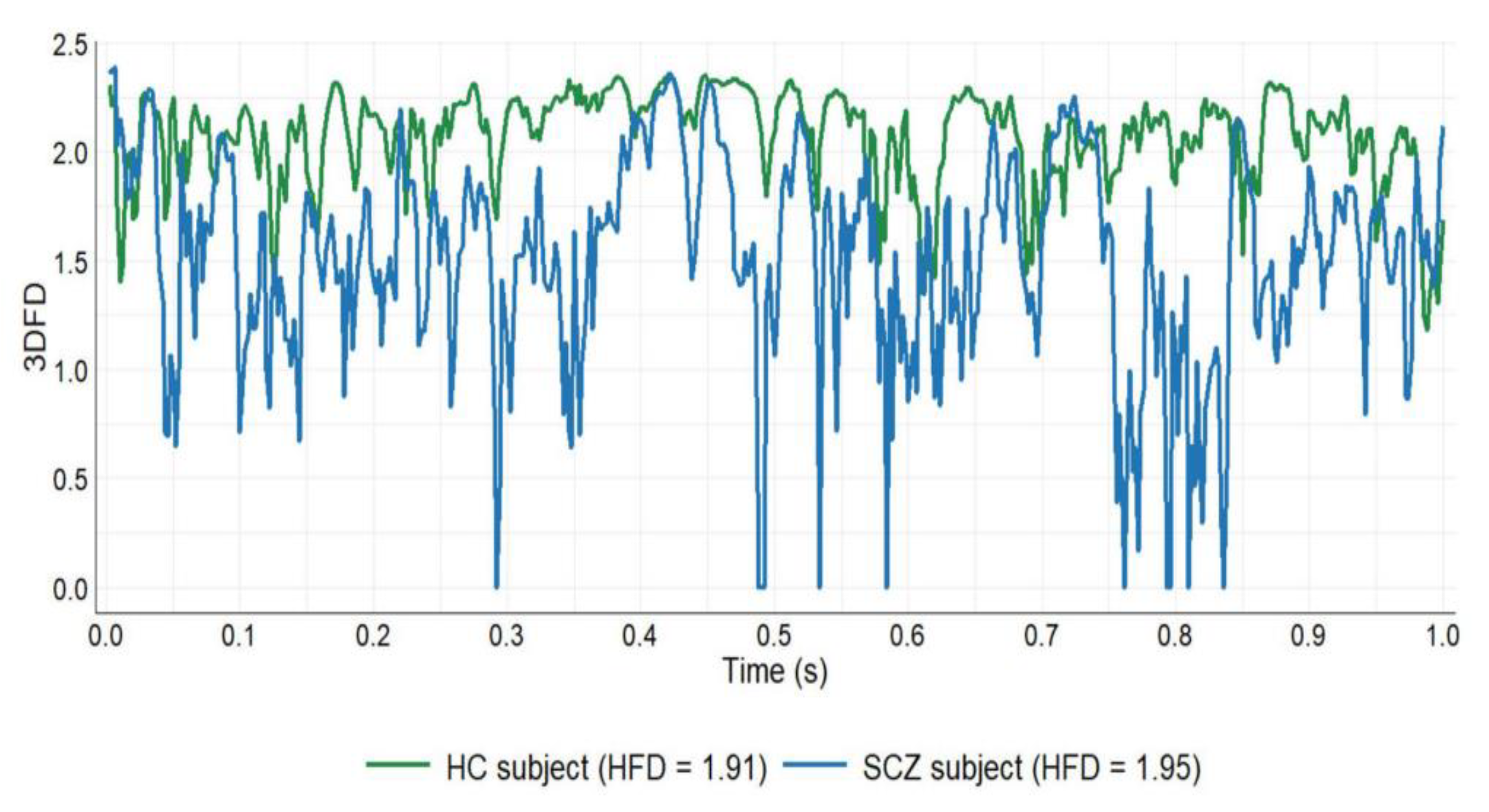
Figure 57.
Sandstone.
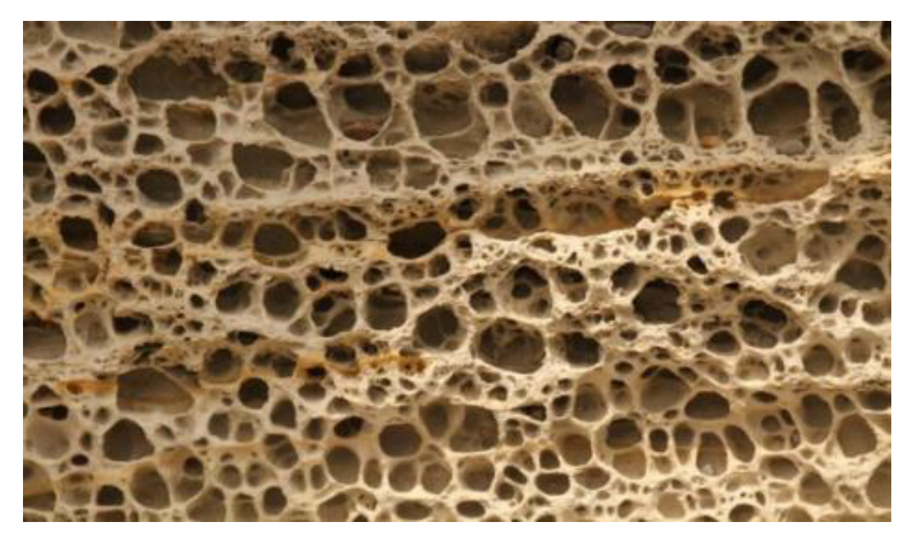
Figure 58.
Bone.
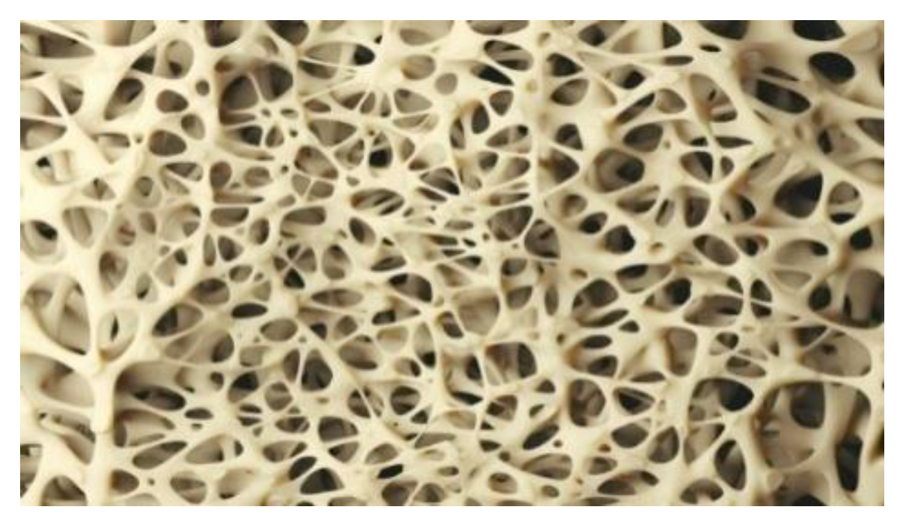
Figure 59.
Craced Farmland.
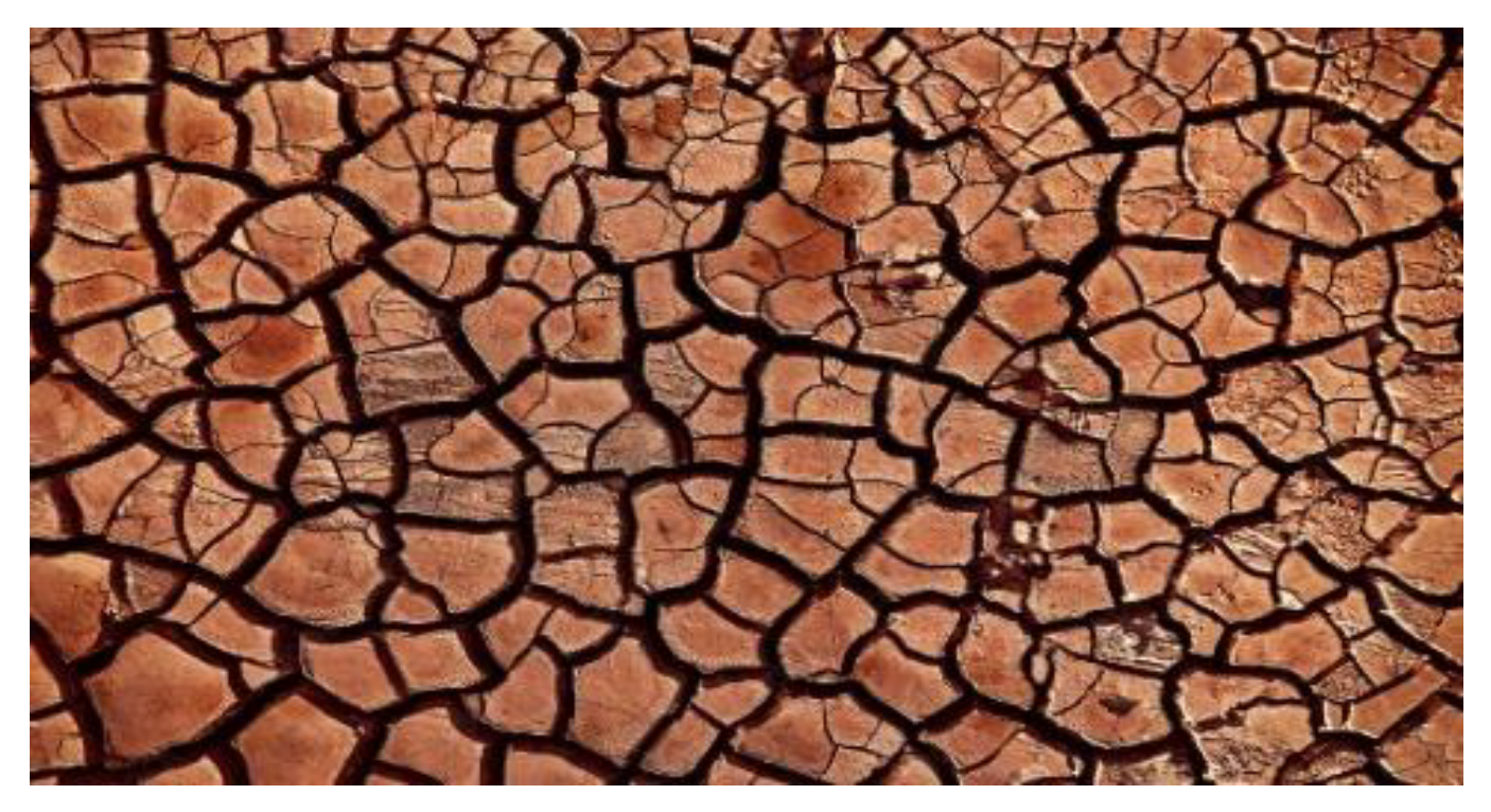
Figure 60.
Graiff fur.
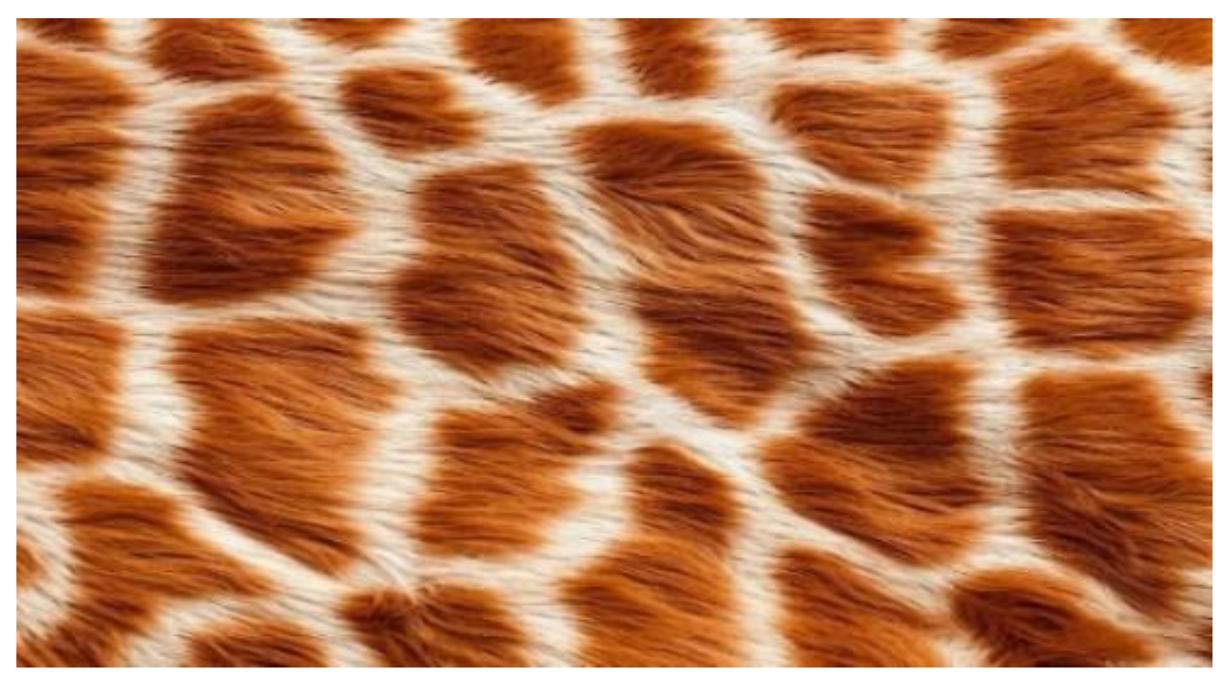
Figure 61.
Lichtenberg figures.
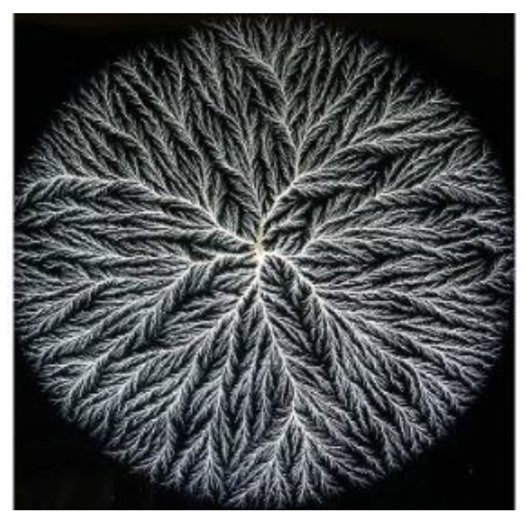
Figure 62.
Bacteria colony.
Disclaimer/Publisher’s Note: The statements, opinions and data contained in all publications are solely those of the individual author(s) and contributor(s) and not of MDPI and/or the editor(s). MDPI and/or the editor(s) disclaim responsibility for any injury to people or property resulting from any ideas, methods, instructions or products referred to in the content. |
© 2024 by the authors. Licensee MDPI, Basel, Switzerland. This article is an open access article distributed under the terms and conditions of the Creative Commons Attribution (CC BY) license (http://creativecommons.org/licenses/by/4.0/).
Copyright: This open access article is published under a Creative Commons CC BY 4.0 license, which permit the free download, distribution, and reuse, provided that the author and preprint are cited in any reuse.


