
Submitted:
12 December 2024
Posted:
19 December 2024
You are already at the latest version
Abstract
The ability of a cell to keep its volume constant irrespective of intra- and extracellular conditions is essential for cellular homeostasis and survival. The purpose of this study is to elaborate a theoretical model of cell volume homeostasis and to apply it to the simulation of human aqueous humor (AH) production. The model assumes a cell with a spherical shape and only radial deformation. The cytoplasm is described as a homogeneous mixture containing fluid, ions and neutral solutes whose evolution is determined by net production mechanisms occurring in the intracellular volume and by water and solute exchange across the membrane. Averaging the balance equations over the cell volume leads to a coupled system of nonlinear ordinary differential equations (ODE) which are solved using the θ-method and the Matlab function ode15s. Simulation tests are conducted to characterize the set of parameters corresponding to baseline conditions in AH production. The model is subsequently used to investigate the relative importance of (a) impermeant charged proteins; (b) sodium-potassium (Na+/K+) pumps; and (c) carbonic anhydrase (CA) in the AH production process. Results suggest that (a) and (b) play a role whereas (c) does lack significant weight, at least for low carbon dioxide values. Model results describe a higher impact from charged proteins and Na+/K+ ATPase than CA on AH production and cellular volume. The computational virtual laboratory provides a method to further test in vivo experiments and machine learning-based data analysis towards the prevention and cure of ocular diseases such as glaucoma.
Keywords:
Homeostasis
; cell volume
; homogeneous mixtures
; mathematical modeling
; aqueous humor production
1. Introduction
The mechanical integrity of a cell is essential to its function and the tissues and organ systems that it supports [1,2]. Cell volume stabilization is a fundamental function to preserve the mechanical integrity of a cell [3]. Cell volume stabilization along time is based on the balance among forces acting on the cell membrane which emanate from electrochemical and fluid-mechanical mechanisms [4]. The experimental characterization of force equilibrium at the nanoscale level is a highly complex task because of the difficulty of performing measurements in vivo (see [5]), and the presence of two regimes of mechanical behavior in living cells, at short and long time scales (see [6]).
Based on these considerations, we address in this article the theoretical study of cell volume dynamics and apply the formulation to the process of production of aqueous humor (AH) in the eye. AH is a slowly moving fluid that is continuously produced by the ciliary body of the eye, whose main function is to keep the anterior segment of the eye clean from metabolic wastes and to preserve the spherical shape of the eyeball by establishing the intraocular pressure (IOP) (see [7,8,9,10]).
Keeping IOP within normal levels (10 to 21 mmHg) is central to prevent the occurrence and progression of neurodegenerative diseases of the retina such as glaucoma [11,12,13]. This opens up the question to understand the biophysical mechanisms that determine the value of IOP and, consequently, the causes of the pathology, and to devise effective therapies for its cure. In this respect, the development of a mathematical model and of a computational virtual laboratory (CVL) for the simulation of AH production has been object of investigation in recent years (see [14,15,16,17]).
In this article, we propose a theoretical formulation based on homogeneous mixtures including neutral and charged solutes (see [18], Chapter 13) and utilizing a model reduction procedure from three spatial dimensions to zero spatial dimensions. The model resulting from reduction is a coupled system of highly stiff nonlinear ordinary differential equations (ODE) which are solved using the -method and the Matlab function ode15s. Simulation tests are run to characterize the values of model parameters at baseline conditions in AH production. The model is subsequently used to investigate the relative importance of (a) impermeant charged proteins; (b) sodium-potassium pump; and (c) carbonic anhydrase in the AH production process. Results suggest that (a) and (b) play a role whereas (c) does not have a significant weight, at least for low CO2 values.
2. Materials and Methods
In Section 2.1 we describe the geometrical representation of the cell volume and surface; in Section 2.2 we describe the heterogeneous structure of the cell membrane; in Section 2.3 we provide a conceptual scheme of transport of water and solute across the cell membrane. In Section 2.4 we introduce a continuum model of the cell based on the theory of mixtures, to describe the spatial and temporal response of the cell volume to the concomitant action of fluid and electrochemical forces. In Section 2.5 we derive a reduced-order model of the cell volume that comprises ordinary differential and algebraic equations. Finally, in Section 2.6 and Section 2.7 we describe the compact form of the reduced-order model and its numerical approximation, respectively. In Appendices Appendix A and Appendix B, we provide the expressions of the fluid velocity, molar flux densities and net production rates that are involved in cellular metabolism.
2.1. Geometrical Description of the Cell
Let denote the time variable (units: s). We denote by the three-dimensional (3D) body representing the cell at time t and the volume of the cell at time t, such that is the value of the cell volume at time , being the cell radius in the initial (undeformed) configuration (units: m). From the point of view of Continuum Mechanics the body is a deformable, electrically charged, homogeneous mixture comprising a fluid constituent, moving charged solute constituents (ions) and moving neutral solute constituents (see [18], Chapter 13). The cell volume contains also impermeant charged proteins whose chemical valency and molar density is such that electroneutrality holds in ionic homeostasis conditions (see [3] and [19]). The boundary of is denoted by and is the outward unit normal vector on . The surface of the cell at time t is denoted by , such that is the value of the cell surface at time . In the remainder of the article, we denote by the spatial coordinate vector of any point of the cell with respect to a fixed system of reference. We also refer to the interior of as the intracellular region (shortly, ), to the exterior of as the extracellular region (shortly, ) and to the surface of as the membrane (shortly, m).
Assumption 1.
We assume that cell deformation occurs only in the radial direction and that it does not depend on the position on the cell surface.
Assumption 2.
We assume that the electric potential, solute concentrations and fluid pressure in the extracellular region are given functions of space and time.
Figure 1 illustrates in solid line and dashed line the initial and deformed configurations of the cell, respectively. In agreement with Assumption 1, both configurations are spherical.
2.2. Porous and Lipid Structure of the Cell Membrane
The intra and extracellular regions are separated by a 3D membrane whose thickness is such that the ratio is . In the limit , the geometrical representation of the 3D membrane degenerates into the two-dimensional (2D) manifold . The membrane surface can be represented as an heterogeneous porous medium whose solid constituent is lipid material. The lipid surface is impermeable to water and solutes whereas the pore surface allows the exchange of fluid and solutes between intra and extracellular regions. The pore surface contains a variety of membrane proteins, denoted by . Each membrane protein is characterized by a dimensionless function , henceforth referred to as surface fraction, defined as
where is the total area occupied by the protein at time t.
Assumption 3.
Let . We assume that
Equation (1b) implies that
The first type of membrane protein that we introduce in this article is the aquaporin (AQP), which is a specialized protein for rapid transmembrane water exchange between intracellular and extracellular regions (see [20,21,22]). The quantity represents the AQP surface fraction. Other membrane proteins on the cell surface comprise carrier proteins, which permit neutral solute exchange through the cell membrane by the mechanism of facilitated diffusion (see [23] and [24]), and ion channels, ion exchangers and ion pumps, which permit charged solute exchange through the cell membrane (see [25]). The total surface fractions for each considered membrane protein are defined as:
in such a way that the total pore surface fraction is
The remainder of the cell surface is occupied by the lipid constituent of the membrane, whose surface fraction is
Assumption (3) implies that the membrane protein surface fractions in (2) do not depend on time, and that also the lipid surface fraction does not depend on time because of (4).
2.3. Water and Solute Transport Across the Cell Membrane
In this section we provide a conceptual scheme of transport of water and solute across the cell membrane and we refer to [21] and [26] for more details about the subject.
Figure 2 illustrates a schematic representation of a zoomed view of the cell membrane and of the intra and extracellular regions. The scheme shows water molecules and solutes (neutral and charged) in motion across the membrane.
Assumption 4.
Based on the scheme in Figure 2 we make the following assumptions:
- A1.
- Water is transported across the membrane, in a selective manner, via aquaporins;
- A2.
- Water and solutes are co-transported across the membrane via ionic channels and carrier proteins;
- A3.
- Water velocity inside ionic channels and carrier proteins is the same as water velocity inside aquaporins.
2.4. Continuum-Based Model of the Cell
This section is structured in four subsections devoted to fluid motion, neutral and charged solutes, and electric potential.
2.4.1. Fluid Motion
Assumption 5.
We assume that water flow is slow and inertial forces can be neglected with respect to the viscous effects.
According to Assumption 5, the motion of water flow across the cell membrane can be described by the linear Stokes equation system (see [18], Section 10.5.1):
where (units: ) and p (units: ) are the fluid velocity and pressure inside the aquaporin, respectively, is the fluid stress tensor (units: ), is the force density acting on the fluid (units: ), is the fluid dynamic viscosity (units: ) and is the symmetric gradient operator.
Equation (5a) expresses mass conservation in local form; equation (5b) expresses linear momentum balance in local form; equation (5c) is the constitutive law for a Newtonian fluid.
2.4.2. Neutral solutes motion
We denote by the set of neutral solutes, with . Each solute is described by its number density and molar density (units: ). The advection-diffusion model is adopted to represent the motion of neutral solutes across the cell membrane (see [18], Chapter 12):
Equations (6a) express mass balance in local form for each solute . The vector is the molar flux density of solute (units: ) accounting for a passive advective contribution due to water motion inside the carrier protein channel (see Assumption 4-A2), and a diffusive contribution expressed by Fick’s law in which is the diffusion coefficient of solute (units: ). The scalar functions and represent production and consumption rates of (units: ).
2.4.3. Charged solutes motion
We denote by the set of charged solutes (ions) with . Each ion is described by its number density , molar density , charge number , diffusion coefficient and electric mobility (units: ). The number and molar densities are related by the equation (units: ), where is Avogadro’s constant. The diffusion coefficient and the electric mobility are proportional through Einstein’s relation
where is the thermal voltage (units: V), , T and q denoting Boltzmann’s constant, absolute temperature and electron charge, respectively. The Nernst-Planck (NP) model is adopted to represent ion transport and exchange across the cell membrane (see [18], Chapter 13):
Equations (8a) express mass balance in local form for each ion . The vector is the molar flux density of ion , accounting for a passive ion molar flux density and an active ion molar flux density . The vector is the velocity-extended NP equation for ion electrodiffusion and accounts for a passive advective contribution and a diffusive contribution expressed by Fick’s law (see [18], Chapter 13). The vector field is the generalized drift velocity of ion due to water motion inside the ion channel (see Assumption 4-A2) and Faraday’s law under quasi-static approximation (see [18], Chapter 14)
where and are the electric field (units: ) and electric potential (units: V), respectively.
The vector expresses passive ion exchange mediated by transporters and co-transporters. The scalar functions and represent production and consumption rates of .
2.4.4. Electric potential
The spatial and temporal distribution of the electric potential across the cell membrane is described by the following differential system:
where is the dielectric permittivity of the cell membrane lipid layer (units: ) and F is Faraday’s constant (units: ). Equation (9a) is a consequence of Maxwell’s equations (see [27] and [18], Chapter 4) and expresses the continuity of the total electric current density (units: ), given by the sum of the total conduction current density and the displacement current density , in which the electric field is expressed as a function of the electric potential via equation (8f).
2.5. Cell Reduced-Order Model
This section is structured in five subsections devoted to the derivation of the reduced-order model for cell surface normal velocity, cell volume, neutral and charged solute molar densities and electric potential.
2.5.1. Time evolution of normal velocity across a single AQP
We make the following assumption on the geometry of the AQP shown in Figure 2.
Assumption 6.
The AQP is geometrically represented as a cylinder with radius and axial length as depicted in Figure 3.
Moreover,
Assumption 7.
We assume that:
- 1.
- the fluid velocity has only the axial component ;
- 2.
- , with and ;
- 3.
- (Poiseuille flow);
- 4.
- the force density has only the axial component ;
- 5.
- , with and .
Inserting Assumptions A7 into equations (5) we obtain the following expression of the normal fluid velocity inside the pore channel of the AQP
Integrating (10a) we get
For any function , we define the transmembrane difference operator
Setting in (10b) and applying the definition (10c) to the variables p and , we obtain
where
is the hydraulic conductivity of the membrane (units: ) and
is the total osmo-oncotic pressure, C being an arbitrary integration constant. Relation (10d) is Starling’s equation [28] and represents the mathematical expression of the normal fluid velocity across the single aquaporin.
2.5.2. Time Evolution of Cell Surface Normal Velocity
In order to determine the motion of the whole cell surface, we need to define an average normal fluid velocity to represent the collective contribution of the AQPs. To this purpose, we denote by the surface density of aquaporins, defined as the number of AQPs per square meter, and by the total surface area occupied by the AQPs. Using Assumption 3, we obtain
Let us introduce the total water volumetric flow rate across the cell surface (units: )
and the average normal fluid velocity across the cell surface
where is given by (11a) and is given by (10d).
The pore fluid velocity is typically quite large (even thousands of , see [29]) to favor a fast transmembrane exchange of water molecules. The average normal fluid velocity , instead, is considerably smaller (less that , see [30]). For this reason, in the remainder of the article, we introduce the following definition.
Definition 1.
Let us denote by the cell surface normal velocity. We set
where is defined in (10d).
2.5.3. Time evolution of cell volume
The time evolution of is described by the cell mass balance equation in integral form (see [18], Chapter 6)
where is the mass density of water (units: ), is the mass of the cell at time t (units: ), and
is the intracellular water mass density net production rate, and being water mass density production and consumption rates, respectively (units: ).
Assumption 8.
We assume that:
where and represent the time-dependent intracellular water mass density production and consumption rates, and the shape function Φ is such that
Using Tr.1 in Assumptions A4, using Definitions 1 and A8 into the right-hand side of (13), and noting that , with , we obtain the following reduced-order model of cell volume motion:
where is given by (10d) and
is the water volume net production rate (units: ), having set and for every .
2.5.4. Time Evolution of Neutral Solutes
The time evolution of neutral solute molar density is described by the mass balance equation in integral form
where is the normal molar flux density of over the cell surface , and
is the net production rate of intracellular solute , and being production and consumption rates, respectively (units: ).
Assumption 9.
We assume that:
where and are time-dependent intracellular neutral solute molar densities and normal molar flux densities over the cell surface, respectively, and the shape function is such that
where is the surface fraction of the carrier protein that allows the transmembrane exchange of the neutral solute β. We also assume that equations similar to (15) apply to and .
Using Assumptions A9 in (13c) we obtain the following reduced-order model for each neutral solute molar density:
where is the initial value of the intracellular neutral solute molar density, , and
is the net production rate of solute (units: ).
2.5.5. Time evolution of charged solutes
The time evolution of charged solute molar density is described by the mass balance equation in integral form
where is the normal molar flux density of over the cell surface , and
is the net production rate of intracellular ion , and being production and consumption rates, respectively (units: ).
Assumption 10.
We assume that:
where is the time-dependent intracellular molar density of ion , the functions and are time-dependent normal molar flux densities over the cell surface representing passive ion transport and exchange, respectively, the function is a time-dependent normal molar flux density over the cell surface representing ion exchange through active pumps, and the shape functions , and are such that:
where , and are the surface fractions of the membrane protein associated with passive transport, passive exchange and active pump-mediated exchange of ion α, respectively. We also assume that equations similar to (8) apply to and .
Using Assumptions A10 in (21) we obtain the following reduced-order model for each charged solute molar density:
where is the initial value of the intracellular charged solute molar density, , and
is the net production rate of ion (units: ).
2.5.6. Time evolution of membrane potential
For any , the membrane potential is defined as
The time evolution of the membrane potential is described by the charge balance equation in integral form
where and are the normal derivative of the electric potential and the normal total conduction current density over the cell surface , respectively.
Assumption 11.
We assume that the electric potential is a piecewise linear continuous function across the cell membrane thickness (see Figure 4).
Using Assumption 11 into the left-hand side of (26), we get
where
is the cell specific capacitance (units: ). The right-hand side of (26) is given by the following expression
where is the total conduction current flowing across the cell membrane at time t (units: A), defined as
Replacing (27) and (29) into (26) we obtain the following reduced-order model for the membrane potential:
where
is the normal total conduction current density over the cell surface defined in (24b), and is the initial value of the membrane potential.
2.6. Compact Form of the Cell Reduced-Order Model
Let us introduce the vector of dependent variables:
where:
are the column vectors containing the time values of neutral and charged solute molar densities.
Let us define the vector of source terms:
where and are column vectors of size and , respectively, containing the time values of neutral and charged solute normal molar flux densities, whereas (and ), (and ) are column vectors of size and , respectively, containing the time values of intracellular neutral and charged solute production (and consumption) terms.
Finally, let us define the column vector containing the initial condition of the model:
where and are column vectors of size and , respectively, which contain the values of the initial conditions for the intracellular neutral and charged solute molar densities.
The equation system constituting the model of cell volume motion can be written in compact form as:
System (37) comprises differential equations and algebraic equations, represented by the constitutive laws for the normal molar flux densities of neutral and charged solutes and for the production and consumption rates of water and solutes. The expressions of the normal fluid velocity on the cell surface and normal molar flux densities are provided in Appendix A whereas the expressions of production and consumption rates are provided in Appendix B.
2.7. Numerical Approximation
The mathematical model proposed in this article is implemented within a Computational Virtual Laboratory (CVL) for the simulation of cell volume motion.
The -method (see [18], Chapeter 3) and the Matlab tool ode suite are used for the numerical approximation of (37) (see [31]). In the case of -method, the values and are utilized, corresponding to the Backward Euler (BE) method and corresponding to the Crank Nicolson (CN) method. In the case of the Matlab tool ode suite, the functions ode15s or ode23tb are utilized because they are specifically tailored to solve stiff problems like the one object of the present article (see [32], Chapeter 11). The function ode15s is endowed with a variable-order Backward Differentiation Formulae (BDF) method, whereas the function ode23tb uses the trapezoidal rule coupled with a BDF of order 3.
The CVL allows the user to consider physical situations of increasing complexity, starting from the solution of the sole Cauchy problem (16) in which the fluid velocity is a given function of time and the production and consumption terms are functions of time and cell volume. Simulation complexity can be increased by adding charged and neutral solutes, intracellular reactions and transmembrane ion exchange mechanisms, as well as the presence of impermeant protein charges in both intra and extracellular regions. This hierarchy of scenarios is investigated in Section 3 where the accuracy and reliability of model predictions is verified against analytical solutions and available data.
3. Results
In this section we validate the proposed CVL through the solution of case studies characterized by an increasing complexity.
3.1. The Basic Configuration
This case study is mathematically represented by the sole model for cell volume motion (16).
Assumption 12.
We make the following assumptions:
- 1.
- for all , being a given constant;
- 2.
- for , being a given positive constant (units: );
- 3.
- for , (units: ) and (units: ) being given positive constants.
Replacing the assumptions on the water volume production and consumption rates ino (16d) we get
Replacing Assumptions 12 and (38) into (16a), we obtain the following Cauchy problem:
where is the cell volume in resting conditions.
The equilibrium points of system (39) are the solution of the following nonlinear algebraic equation
where is the dependent variable and is the stationary value of the cell volume.
Figure 5 (left panel) shows a graph of f in correspondance of the following values of the input data: , , , and . System (39) admits two equilibrium points: and . We have
from which we can conclude that is the only stable equilibrium point of system (39). The theoretical conclusions of the stability analysis are confirmed by Figure 5 (left panel) which shows the normalized cell volume computed by solving system (39) in the time interval with the following values of model parameters: , , , and . Cell volume dynamics was studied using the BE method on a uniform time partition made of elements. Consistent with the physical configuration illustrated in Figure 1, the cell tends to increase its volume by more than 60% because of the inflow of water from the extracellular region. Cell volume reaches a stationary limit because of dominating intracellular water consumption over intracellular water production.
Figure 6 (left panel) illustrates the temporal evolution of cell volume in the case where the values of are . The black arrow in each figure indicates the increase of , from negative to positive values. Results suggest that the cell switches between swelling and shrinking as fluid velocity changes its sign from negative to positive. Interestingly, the BE method gives rise to positive cell volumes for each and for each considered value of . This outcome is the consequence of the positivity principle enjoyed by the BE method when applied to the linear equation for , being a given positive constant. The difference between using the BE method () and another -method with is illustrated in Figure 6 (right panel) which shows a comparison between the BE method (red line) and the Crank Nicolson method (CN, blue line) in the solution of (39) when the time interval is , the fluid velocity is and the number of time elements is 10, corresponding to a time step . The value of the remaining model parameters is the same as in the previous example. Results indicate that the solution computed by the CN method is affected by spurious unphysical oscillations unlike that computed by the BE method. Such oscillations can be removed by increasing the number of discretization time elements, at the price of increasing the computational effort.
Figure 7 (left panel) illustrates the temporal evolution of the water volume net production rate in the time interval with the fluid velocity varying in the range . We see that the stationary value of , for each considered normal fluid velocity in the range , changes from negative to positive, the magnitude for being three times larger than for . Figure 7 (right panel) illustrates the temporal evolution of the cell normalized volume in the time interval (ten times smaller than before) in the case where for and the fluid velocity varies in the range . We see that in the absence of intracellular regulatory mechanisms, model system (39) predicts an abnormal increase of cell volume for a highly negative value of normal fluid velocity.
3.2. Cell Homeostasis in the Ciliary Epithelium of the Eye
This case study is mathematically represented by the Cauchy problem (37) in which the cell represents one of the pigmented/nonpigmented couplet in the ciliary epithelium (CE) of the ciliary body of the eye (see [7,8,33]). The aim of the study is to apply the model proposed in this article to characterize the homeostatic configuration of the cell under physiological conditions of the system. According to the data reported in [7], such conditions correspond to:
- (i)
- volume of the CE equal to ;
- (ii)
- number of the cell couplets constituting the CE equal to 4 millions;
- (iii)
- intraocular pressure equal to ;
- (iv)
- AH volumetric flow rate equal to .
Assumption 13.
We make the following assumptions:
- 1.
- the considered sets of neutral and charged solutes are:
- 2.
- the molar densities of neutral and charged solutes are given constants denoted by , , and , ;
- 3.
- the hydraulic pressure difference is a given constant denoted by ;
- 4.
- no transmembrane ion exchangers are considered, so that ;
- 5.
- the model of carrier membrane proteins is described in Appendix A.2;
- 6.
- the model of ion channels is described in Appendix A.3;
- 7.
- the model of net production rates for neutral and charged solutes is described in Appendix B.1;
- 8.
- the model of net production rate in cell volume regulation is described in Appendix B.2.
The values of all model parameters that are used in the computer simulations illustrated in this section are listed in Table 1.
The vector containing the initial condition data is
The vectors containing the extracellular values of the solute molar density are:
The values of the remaining model parameters can be found in Appendix B.1, Appendix B.2 and Appendix B.3. Computations are done using the Matlab solver ode15s setting both relative and absolute tolerances equal to .
3.2.1. Electroneutrality and Impermeant Charged Proteins
Electroneutrality is essential in the maintainance of cell volume as a function of time and of phenomena occurring in the intracellular and extracellular regions (see [3] and references cited therein). Computation of the total electric charge densities and due to mobile ions inside and outside the cell at resting conditions yields:
These results indicate that the intracellular region (at ) is characterized by a high excess of positive charge whereas the extracellular region (at ) is characterized by a high excess of negative charge. This charge difference gives rise to a large osmotic pressure difference across the cell membrane which may eventually lead to disruption of cell integrity. To neutralize the excess of positive and negative charge, we need the presence of internally sequestered impermeant charges inside and outside the cell. Denoting by and the molar density and charge number of the impermeant charge, we have:
These results indicate that a high molar density of fixed anions is sequestered inside the cell cytoplasm whereas a much smaller molar density of cations is required to make the extracellular solution electroneutral.
Assumption 14.
We assume that the number of moles of intracellular impermeant charge is constant during the time evolution of the cell.
Let denote the intracellular molar density of the impermeant charge at time (units: ). By definition of molar density, we have
Using Assumption 14 and (44), we can express the intracellular impermeant charge molar density for any time as
Simulations illustrated in the next sections are conducted using the values of and in (43) and the constitutive equation (45).
3.2.2. Fast Time Scale Cell Evolution
We investigate the evolution of the cell in the time interval , where and .
Figure 8 (left panel) illustrates the time evolution of the intracellular protonated hydrogen (blue curve) and the corresponding intracellular pH (red curve). Hydrogen fast diffusion from the intracellular side into the extracellular side determines a sharp decrease of so that the cytoplasm solution turns into a very basic condition (the maximum value of intracellular pH is 12.5). Figure 8 (right panel) illustrates the time evolution of the average cell normal surface velocity (blue curve) and the corresponding percentage variation of the cell volume with respect to the initial condition (red curve). Cell surface velocity is positive and very small in magnitude (less than ) so that the volume of the cell experiences a very little decrease (maximum magnitude equal to ) with respect to resting conditions. Figure 8 (middle panel, bottom) illustrates the time evolution of the total AH volumetric flow rate throughout the CE (units: ). The quantity is computed for every using the following relation
In less than 50ps, reaches almost 72% of the volumetric flow rate that is physiologically expected in a normal tension individual (see condition [(iv]).
3.2.3. Medium Time Scale Cell Evolution
We investigate the evolution of the cell in the time interval , where and .
Figure 9 (top left panel) illustrates the time evolution of the intracellular CO2 (blue curve) and H2CO3 (red curve) molar densities. In less than 0.5s the hydration process gives rise to a significant production of carbon dioxide and carbonic acid, which is eventually followed up by a stationary condition corresponding to the dynamic equilibrium of reaction (A6a). The consequence of the CO2 hydration can also be seen from Figure 9 (top right panel) that illustrates the time evolution of the intracellular H+ molar density and the corresponding pH (blue and red curves, respectively). Protonated hydrogen concentration increases significantly until almost because of carbonic acid dissociation (forward reaction in (A6b)). Then, the association reaction (backward reaction in (A6b)) with bicarbonate gives rise to a decrease of until a stationary condition is reached. In such a condition, the value of the intracellular pH (almost 6) indicates that the cytoplasm solution is acid. Figure 9 (bottom left panel) illustrates the time evolution of the average cell normal surface velocity (blue curve) and the corresponding percentage variation of the cell volume with respect to the initial condition (red curve). As in the fast scale cell evolution, the cell surface velocity is positive and very small in magnitude (less than ). In this case, however, the much larger time duration of the analysis (5 seconds instead of 50ps) allows the cell to decrease by a larger percentage amount with respect to resting conditions (less than instead of ). Figure 9 (bottom right panel) illustrates the time evolution of the total AH volumetric flow rate throughout the CE (units: ). In 5s, reaches more than 78% of the volumetric flow rate that is physiologically expected in a normal tension individual.
3.2.4. Long Time Scale Cell Evolution
We investigate the evolution of the cell in the time interval , where and . The value of corresponds to the time that is needed by the eye to completely replace the AH content of the anterior chamber (see [7] and [9]).
Figure 10 (top left panel) illustrates a zoomed view of the time evolution of the membrane potential in the time interval . After an initial ultra-fast transient due to the mismatch between the intracellularly applied initial conditions and the conditions in the extracellular bath, the cell reaches a stationary state of , corresponding to an after-hyperpolarization of . Figure 10 (top right panel) illustrates a zoomed view of the time evolution of the intracellular molar densities of sodium (blue curve), potassium (red curve) and chlorine (green curve) for . The concentration of sodium experiences a significant depletion (from 10 to 5.4 mM) because of the NaK ATPase pump activity. Similarly, the concentration of potassium increases from 140 mM up to a stationary value of almost . The green curve in Figure 10 (top right panel) indicates that the concentration of intracellular chlorine experiences a depletion from 7mM to 5.3mM. This can be explained by Figure 10 (middle left panel) which illustrates a zoom of the chlorine molar flux density (units: ) for . The positive value of indicates that chlorine is swept out of the cell cytoplasm with a progressively reducing magnitude along time. Figure 10 (middle right panel illustrates a zoom of the time evolution of the average cell normal surface velocity (blue curve) and the corresponding percentage variation of the cell volume with respect to the initial condition (red curve) for . As in the previous conditions the cell surface velocity is positive and very small in magnitude (less than ). The stationary cell volume percentage decrease with respect to resting conditions is less than . Figure 10 (bottom center panel) illustrates a zoom of the time evolution of the total AH volumetric flow rate throughout the CE (units: ) for . The stationary value of is 2.75017 , with a percentage error of -0.0062 % with respect to the physiological value of 2.75 .
4. Discussion
Cell volume stabilization is a fundamental function to preserve the mechanical integrity of a cell [3]. Keeping the cell volume constant along time is the result of the balance among forces acting on the cell membrane from both intra and extracellular sides, which emanate from electrochemical and fluid-mechanical mechanisms [4]. The experimental characterization of force equilibrium at the scale of the cell membrane is a nontrivial task, on the one hand, because of the difficulty of performing measurements in vivo (see [5]), and, on the other hand, the presence of two distinct regimes of mechanical behavior in living cells. In fact, a combination of experimentation and theoretical analysis shows that living mammalian cytoplasm behaves as an equilibrium material at short time scales whereas it behaves as an out-of-equilibrium material at long time scales [6].
Based on these considerations, we address in this article the theoretical study of cell volume dynamics with the aim of applying the formulation to the process of production of aqueous humor (AH) in the eye. AH is a slowly moving fluid that is (1) continuously produced by the ciliary body of the eye; (2) flows from the posterior into the anterior chamber of the eye; (3) is drained out of the eye throughout two main outflow pathways (see [7,8,9,10]). The sequence: (1) AH production; (2) AH flow; and (3) AH outflow is schematically represented in Figure 11.
The main function of AH is to keep the anterior segment of the eye clean from the metabolic waste of the surrounding tissues and to preserve the spherical shape of the eyeball by establishing the intraocular pressure (IOP) as the value of AH fluid pressure in correspondance of which the volumetric flow rate of AH that is produced by the ciliary body equals the volumetric flow rate of AH that is drained out by the outflow pathways in the anterior segment of the eye (see [35]). Successful control of the IOP within normal levels (10 to 21 mmHg) is central to prevent the occurrence and progression of neurodegenerative diseases of the retina such as glaucoma [11,12,13]. Therefore, unraveling the biophysical mechanisms that concur to determine the value of IOP may be of significant help to understand the causes of glaucoma and to develop effective therapies for its cure.
The development of a mathematical model and of a CVL for the simulation of the process of production, flow and outflow of AH has been subject of investigation in recent years (see [14,15,16,17]). Our proposed formulation is characterized by the following features: (F.1) it is based on the use of homogeneous mixtures including neutral and charged solutes (see [18], Chapter 13); (F.2) it is defined at the level of the single cell; and (F.3) it utilizes a model reduction procedure from three spatial dimensions to zero spatial dimensions. Feature (F.1) confers a solid theoretical foundation to the proposed model. Features (F.2) and (F.3) make the model structure simple and the computational schemes fast and suitable for adoption in a clinical environment. The model is a consistent generalization of previous approaches [3,4] as it shares with them the same conceptual simplifying assumption of working at the level of the single cell. This assumption is applied here to evaluate the collective behaviour of the cells in the CE of the eye in the process of production of AH.
The model that we propose in these pages has also limitations: (L.1) the dependence of all the variables from the spatial coordinate is neglected; (L.2) several important transmembrane mechanisms regulating solute exchange are not considered in the simulations; (L.3) statistical variability of parameters is not accounted for. Limitation (L.1) is a consequence of the use of the 3D-to-0D reduction procedure. Limitation (L.2) is a choice to prevent proliferation of model parameters thereby rendering easier the analysis of simulation predictions. Limitation (L.3) is a consequence of the choice of using a mechanistic (continuum-based) approach. We intend to remove all of these limitations in future extensions of the formulation considered in the present article.
4.1. The Impact of the Oncotic Pressure Due to the Impermeant Charge
In this simulation we solve system (37) in the time interval with the same set of parameters as in Section 3.2, except the reflection coefficient which is set equal to (Matlab vector notation). By doing so, the weight of the contribution of the oncotic pressure difference (A3h) to the total osmo-oncotic pressure difference (A3k) increases progressively from 0% () to 100 % (), thereby allowing us to investigate the impact of the oncotic pressure difference on AH simulation.
Figure 12 (left panel) illustrates the time evolution of the total volumetric flow rate as a function of time t in the interval . Results indicate that the smaller , the larger the predicted total volumetric flow rate of AH. In particular, the value of predicted by the model that is compatible with the given intracellular and extracellular fluid pressures (20mmHg and 15 mmHg, respectively) is obtained for . To better understand the effect of including properly the impermeant charge in AH modeling, we illustrate in Figure 12 (right panel) the time evolution of the total osmo-oncotic pressure difference in the interval . We see that the magnitude of largely exceeds the contribution from hydrostatic pressure difference (equal to ) for every value of . Moreover, for every the oncotic pressure difference is always positive whereas the total osmotic pressure difference is always negative, so that, as increases, the magnitude of the total osmo-oncotic pressure difference decreases, to reach the value of .
4.2. The impact of the Na+/K+ ATPase
In this simulation we solve system (37) in the time interval with the same set of parameters as in Section 3.2, except the amplification coefficient in (A10e) which is set equal to (Matlab vector notation). By doing so, the weight of the contribution of the sodium/potassium pump to the electrochemical balance of the cell increases progressively from 0% () to 100 % (), with respect to the working conditions of Section 3.2, thereby allowing us to investigate the impact of the Na+/K+ ATPase on AH simulation.
Figure 13 illustrates the time evolution of the total volumetric flow rate as a function of time t in the interval . Results indicate that for (corresponding to values of , the predicted total volumetric flow rate of AH is negative. This means that the pump does not have enough energy to move sodium out from the cell and potassium into the cell, so that the accumulation of sodium in the cytoplasm attracts chlorine from the extracellular region, eventually leading to the inversion of fluid flow. The predicted total volumetric flow rate of AH becomes positive for . This means that the pump does have enough energy to move sodium out of the cell and potassium into the cell, preventing chlorine accumulation in the cell cytoplasm. For increasing values of the ATP concentration () water flux is favored, reaching a physiological level when .
4.3. The impact of carbonic anhydrase
In this simulation we solve system (37) in the time interval with the same set of parameters as in Section 3.2, except the amplification coefficient in Equations (A7c)- (A7d) which is set equal to (Matlab vector notation). By doing so, the weight of the contribution of the CA enzyme to improve the reaction rate of CO2 hydration increases progressively from 0% () to 100 % (), with respect to the working conditions of Section 3.2, thereby allowing us to investigate the impact of the CA enzyme on AH simulation.
Figure 14 illustrates a zoomed detail of the time evolution of the total volumetric flow rate as a function of time t in the interval . Results indicate that is practically independent of the concentration of the CA enzyme. Further tests with higher values of the amplification parameter do not show significant variation of the predicted value of , this probably to be ascribed to the low value of the intracellular carbon dioxide molar density (cf. Figure 9).
4.4. The impact of IOP
In this simulation we solve system (37) in the time interval with the same set of parameters as in Section 3.2, except the value of IOP which is taken in the range [15, 150]mmHg. By doing so, we want to investigate the response of the model in the case of highly hypertensive patients.
Figure 15 illustrates the % difference between at 15mmHg and evaluated in correspondence of IOP in the interval [15, 150]mmHg. The trend is linear with respect to IOP, which agrees with the following expression for fluid velocity
where =20 mmHg is the intracellular fluid pressure (corresponding to the estimated fluid pressure in the CE upon assuming 25mmHg in the ciliary capillaries), and is the total osmo-oncotic difference. Since turns out to be negative with respect to t, as IOP increases, we see from (47) that diminishes, which explains the fact that also diminishes. We notice that for IOP=30 mmHg, which is a typical value of the intraocular pressure in hypertensive individuals, the % difference between at 15mmHg and is 1.09% which increases to 2.54% for IOP=50 mmHg.
5. Conclusions
In this article we have proposed, analyzed and numerically investigated a reduced-order mathematical description of cellular volume homeostasis. The model accounts for intracellular reactions and transmembrane mechanisms for neutral and charged solute exchange. Hydrostatic and osmo-oncotic pressure differences are used in the context of Starling’s Law to compute the velocity of the fluid which drives the motion and radial deformation of the cell volume.
The model is implemented within the context of a CVL that is applied to the study of the process of AH production in the human eye. The scope of the simulations is to test the potential of the CVL to assess the relative quantitative importance of the biophysical mechanisms that underlie AH production, in the perspective of its use as a supporting tool to integrate and complement in vivo experiments and artificial intelligence-based methodologies for the analysis of data on a statistically significant number of patients.
The main conclusions of the model simulations suggest the importance of impermeant charged proteins and Na+/K+ ATPase on the level and direction of AH production, whereas AH production seems to be independent on CA concentration, at least for low values of CO2 concentration.
Author Contributions
Conceptualization, R.S. and G.C.; methodology, R.S.; software, R.S.; validation, R.S., B.S. and G.A.; formal analysis, R.S., A.L. and G.G.; investigation, R.S., G.A.; resources, A.H. and G.G.; data curation, R.S. and K.W.; writing—original draft preparation, R.S.; writing—review and editing, R.S., B.S., A.L., K.W. and A.H.; visualization, R.S.; supervision, A.H.; project administration, A.H. and G.G.; funding acquisition, A.H., A.V., B.S. and G.G.. All authors have read and agreed to the published version of the manuscript.
Funding
This work was partially supported by NIH grants R01EY030851 and R01EY034718, NSF grants 2108711/2327640 and 2412130, NYEE Foundation grants, The Glaucoma Foundation, and in part by a Challenge Grant award from Research to Prevent Blindness, NY. Professor Alon Harris is supported by NIH grants (R01EY030851 and (R01EY034718), NYEE Foundation grants, The Glaucoma Foundation, and in part by a Challenge Grant award from Research to Prevent Blindness, NY. Dr. Alice Verticchio is supported by NYEE Foundation grant.
Conflicts of Interest
The funders had no role in the design of the study; in the collection, analyses, or interpretation of data; in the writing of the manuscript; or in the decision to publish the results.
Abbreviations
The following abbreviations are used in this manuscript:
| AH | Aqueous humor |
| CA | Carbonic anhydrase |
| ATP | Adenosinetriphosphate |
| IOP | Intraocular pressure |
| CVL | Computational virtual laboratory |
| AQP | Aquaporin |
| BE | Backward Euler |
| CN | Crank Nicolson |
| CE | Ciliary epithelium |
Appendix A. Normal Fluid Velocity and Solute Molar Flux Densities
In this section we provide the expressions of the normal fluid velocity on the cell surface and solute molar flux densities in (35).
Appendix A.1. Normal fluid velocity
To determine the normal fluid velocity on the cell surface we consider the following two cases:
- (B.C.1)
- The hydraulic pressure difference is given (units: ).
- (B.C.2)
- The total water volumetric flow rate across the cell surface is given (units: ).
In case (B.C.2) we use (11b) to obtain
In case (B.C.1) we use (10d) to obtain
To determine we need to provide a mathematical model for the total osmo-oncotic pressure difference . Let us define the electrochemical potential of ion
where is a reference molar density. Let us introduce the pressure differences:
The quantities and are the osmotic pressure differences associated with the charged solute and neutral solute , respectively, whereas is the oncotic pressure difference associated with the impermeant charge . The quantity R is the gas constant (units: ), and , and are the membrane reflection coefficients associated with ion , solute and impermeant fixed charge , respectively. We notice that each coefficient is in the range , the value 0 corresponding to a completely permeable membrane and the value 1 corresponding to a completely impermeable membrane. To evaluate the integral on the right-hand side of (A3b) we replace with its spatial average
Postponing to Appendix A.3 the computation of (A3e) and replacing it into (A3b), we get:
We define the total osmotic pressure difference as
and the oncotic pressure difference as
Then, we define the total osmo-oncotic pressure difference as
Relation (A3k) is the generalization of Eq. (31) in [4].
Appendix A.2. Neutral solutes
Let us consider a carrier protein whose geometrical structure is the same as the pore illustrated in Figure 3 in the case of an AQP. To determine the normal molar flux density of solute inside , we make the following assumptions.
Assumption 15.
We assume that:
- 1.
- the molar flux density of the neutral solute β has only the axial component ;
- 2.
- for any , the quantity is spatially constant inside , i.e., , with and .
Using Assumptions A15, Assumption 4-A3 and the fact that is spatially constant, into the constitutive equation (6b) gives the following second-order equation for the solute molar density inside the carrier protein channel
whose solution is
and being time-dependent arbitrary functions. Inserting (A4b) into the constitutive equation (6b) yields
To determine we need to enforce the boundary conditions:
where and are the intra and extracellular values of the neutral solute molar density for any . Using (A4d) into (A4b), we obtain the following expression of the normal molar flux density of inside the carrier protein channel
where is the membrane permeability to the neutral solute (units: ),
is the inverse of the Bernoulli function and
Appendix A.3. Charged solutes
We can proceed in the same way as in Appendix A.2 to obtain the following expression for the normal molar flux density of ion inside an ionic channel
where is the membrane permeability to the charged solute and
Using the definition (8e) of the generalized drift velocity of ion into (A5b) we find the spatial distribution of inside the ionic channel
where and are time-dependent arbitrary functions, and is the average normal component of over the cell surface, and . Replacing (A5c) into (A3e), we obtain
where:
Figure A1.
Red solid line: plot of for and , being a dimensionless time. The endpoint values of are and for every . Black dashed line: arithmetic average of .
Figure A1.
Red solid line: plot of for and , being a dimensionless time. The endpoint values of are and for every . Black dashed line: arithmetic average of .
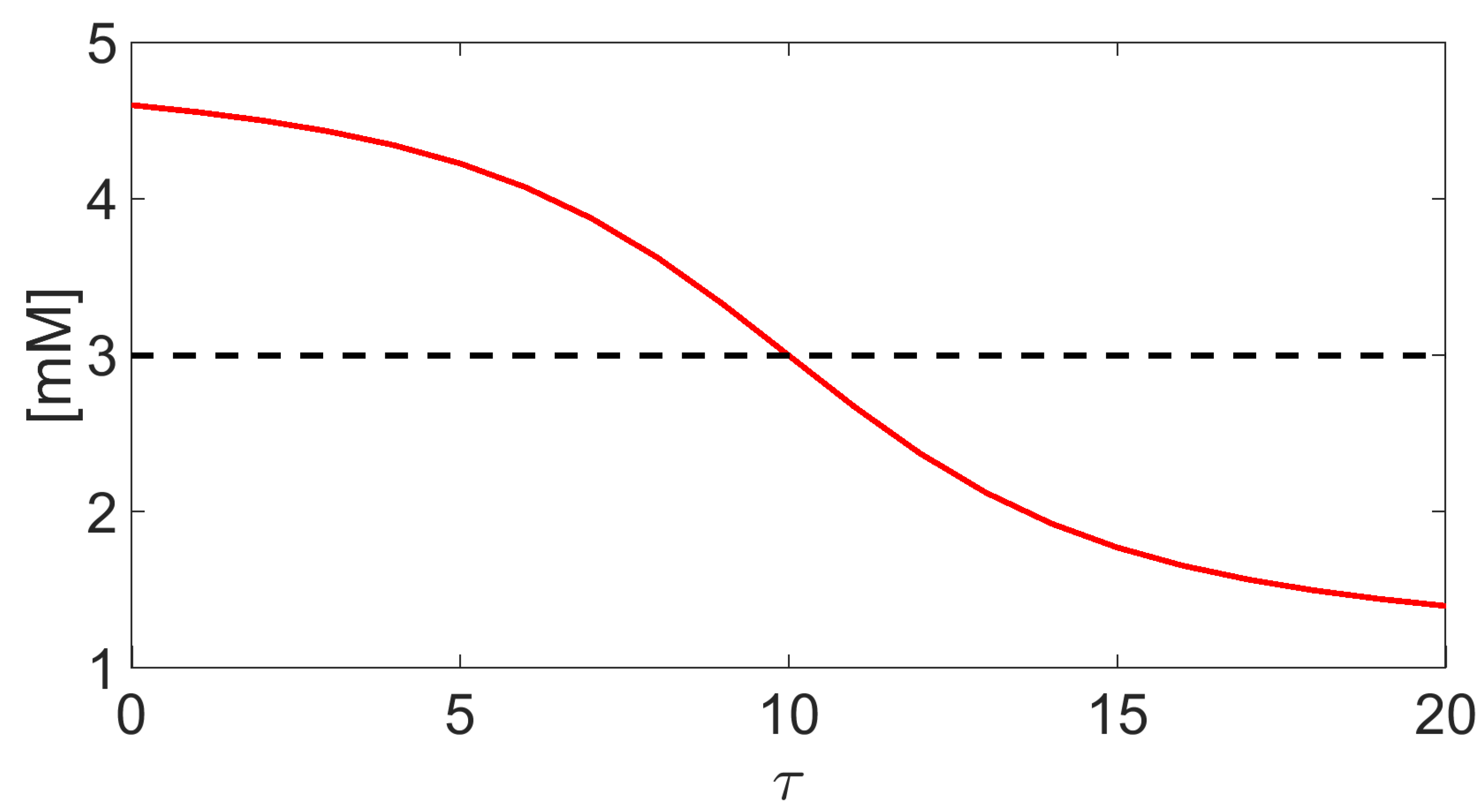
We illustrate in Figure A1 the graphical representation of (red solid line) compared to the arithmetic value for (Matlab vector notation), , and . We see that and are comparably close only if , which corresponds to a diffusive regime of transport inside the channel. Conversely, their distance increases for larger values of , which corresponds to an advection-dominated regime of transport inside the channel. On the basis of these considerations, the adoption of (A5d) instead of the customary choice (as done, for example, in [4]) is expected to warrant an accurate and robust model simulation.
Appendix B. Mathematical Modeling of Cellular Metabolism
The following conceptual scheme of cellular metabolism is considered in this article:
- Glucose is absorbed by mitochondria to produce ATP and CO2.
- ATP provides the energy needed by the Na+/K+ pump to export 3 sodium ions and import 2 potassium ions.
- The carbonic anhydrase enzyme (CA) catalizes the hydrolysis of CO2, which is a waste product of mitochondrial metabolism.
- Specialized exchangers supervise transmembrane transport of proton (H+) and bicarbonate (), which are the products of CO2 hydrolysis.
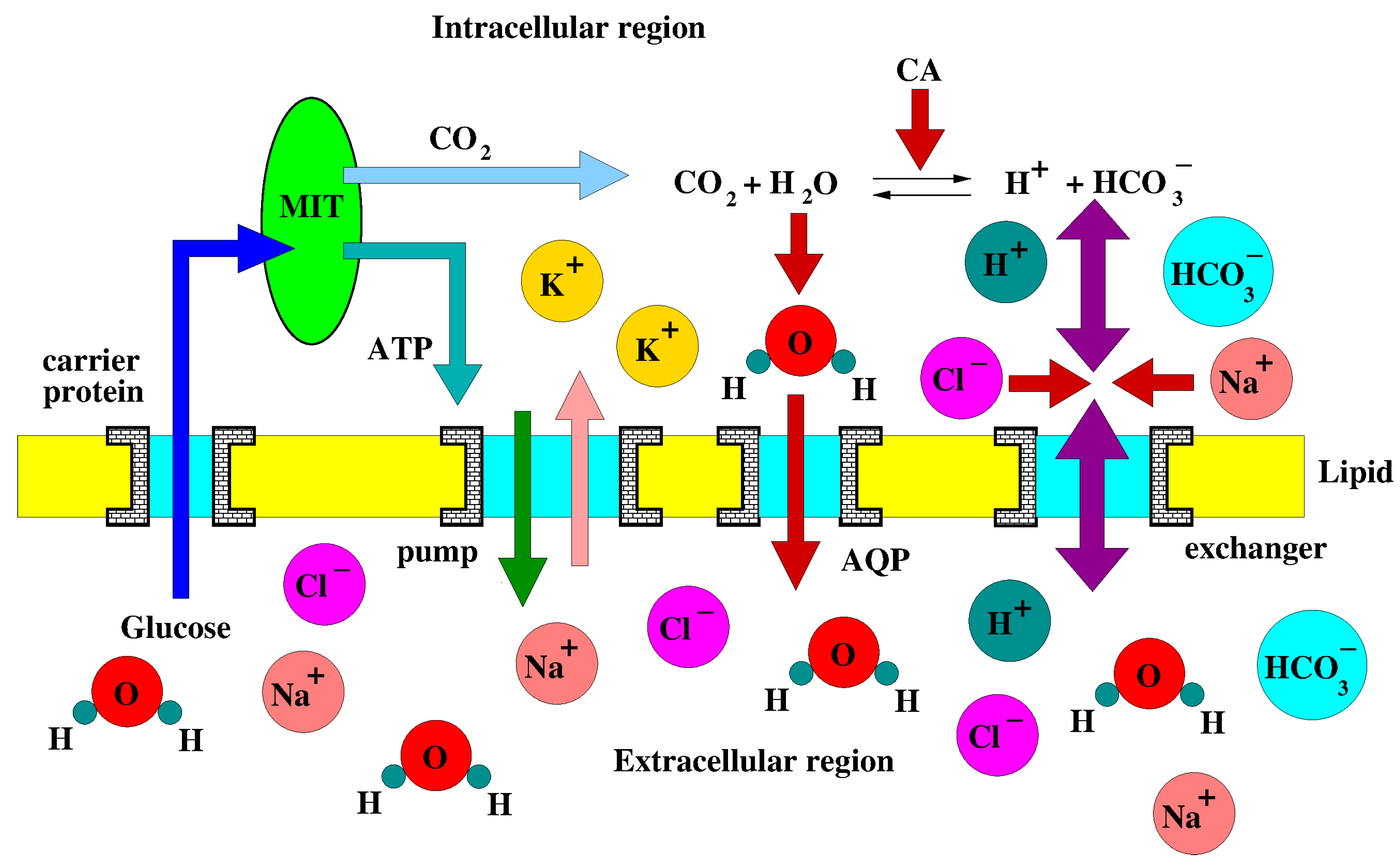
Figure A2 illustrates the intracellular reactions and transmembrane transport mechanisms that are involved in the cellular metabolism.
Figure A2.
Schematic representation of intracellular reactions and transmembrane transport mechanisms. MIT: mitochondrium. ATP: adenosinetriphosphate. CA: carbonic anhydrase. Exchangers perform multiple ion transport across the membrane.
Figure A2.
Schematic representation of intracellular reactions and transmembrane transport mechanisms. MIT: mitochondrium. ATP: adenosinetriphosphate. CA: carbonic anhydrase. Exchangers perform multiple ion transport across the membrane.
In the following, we provide the expressions of:
- the production and consumption rates for the neutral and charged solutes involved in the CA-enzyme-mediated carbon dioxide conversion into carbonic acid and its subsequent dissociation into protonated hydrogen and bicarbonate;
- the production and consumption rates in cellular volume regulation;
- the molar flux densities representing the mathematical model of transmembrane sodium and potassium solute exchange throughout the Na+/K+ ATPase.
Appendix B.1. Mathematical model of CA-mediated CO2 hydrolysis
In this section we illustrate the mathematical modeling of the CA-enzyme-mediated hydrolysis. This process can be conveniently represented as the following two-step chemical reaction (see [36,37]):
STEP 1 is the conversion of intracellular carbon dioxide into carbonic acid under mediation of the CA enzyme, which is a very fast catalyzer of the CO2 hydration process (see [38,39]). STEP 1 is characterized by the quantities and (units: ) depending on the molar density of the carbonic anhydrase enzyme (CA) and representing the rate constants of the forward and backward reactions in STEP 1, respectively.
Assumption 16.
Let denote the molar density of intracellular CO2 that is hydrated by water molecules. We assume that each molecule that is produced by mitochondria respiration is hydrated by a corresponding water molecule. This allows us to denote by the molar density of the intracellular .
Using the Law of Conservation of Mass and Assumption 16, the net production rates in the mass balance equation for and have the following expressions:
The hydration and dehydration rate constants experimentally depend on the amount of CA that is present in the compartment where the hydration reaction takes place (see [40]). Following [36,37], in this article we use the following model for the hydration and dehydration rate constants:
where is a nonnegative given constant, whereas and are experimental reference values measured at reported in [41]. Taking is a way to represent the catalyzing effect of CA compared to the uncatalyzed reaction corresponding to . In the numerical simulations illustrated in Section 3.2 we set .
STEP 2 is the dissociation of intracellular carbonic acid into bicarbonate and protonated hydrogen, and is characterized by the quantities (units: ) and (units: ), the rate constants of the forward and backward reactions in STEP 2, respectively. The dissociation reaction of H2CO3 is extremely rapid, so that the values of the forward and backward rate constants in STEP 2 are very large. In the numerical simulations illustrated in Section 3.2 we use the data of [36,37], and set and , where is the equilibrium constant of STEP 2. Using the Law of Conservation of Mass, we obtain the following expressions for the net production rates in the mass balance equations for and :
Assumption 17.
We assume that ions are non-reacting (see [42], Section 8.3.3). Therefore, we have , .
Appendix B.2. Net production rate in cell volume regulation
The mechanisms which govern intracellular water production/consumption are object of considerable debate and investigation because of their importance in cell life and survival. One example is provided by the process of normotonic cell shrinkage which is the major hallmark of cellular apoptosis [43]. Another example is provided by the TCA cycle (Krebs cycle) in cellular respiration, whose products of metabolism of fuels are ATP, CO2, and the so-called “metabolic” water [44].
The difficulty of accessing and sampling the contents of intact cells makes the study of the intracellular fluid environment, and, more generally, of body fluid content, a challenging problem. Specific approaches to accurately detect metabolic water content as a result of intracellular metabolic activity have been proposed in [45] and [46].
In this article, we focus on the role of net production and consumption of intracellular water in driving the motion of the cell surface. Our proposed model is
where and are given constants (units: ) and is the value of cell volume in resting conditions. In the simulations illustrated in Section 3.2, we set .
Appendix B.3. Na + /K + ATPase
The mathematical model of the sodium-potassium pump (Na+/K+ ATPase) adopted in this article follows the idea proposed in [3]. The molar flux densities for sodium and potassium are:
where:
The quantity is the maximum pump molar flux density (units: , is the intracellular molar density of ATP (units: ) and is the ion transfer velocity of the pump (units: ). The quantities and are defined as:
where is the reference value of ATP molar density (units: ), is pump turnover rate (units: ) and is a nonnegative given constant. The quantities and are the Michaelis constants of the pump model (units: ).
In the simulations illustrated in Section 3.2 we set , , , and .
References
- Cid, V.J.; Durán, A.; del Rey, F.; Snyder, M.P.; Nombela, C.; Sánchez, M. Molecular basis of cell integrity and morphogenesis in Saccharomyces cerevisiae. Microbiological Reviews 1995, 59, 345–386. [Google Scholar] [CrossRef]
- Ammendolia, D.A.; Bement, W.M.; Brumell, J.H. Plasma membrane integrity: implications for health and disease. BMC Biol 2021, 19. [Google Scholar] [CrossRef] [PubMed]
- Armstrong, C.M. The Na/K pump, Cl ion, and osmotic stabilization of cells. Proceedings of the National Academy of Sciences 2003, 100, 6257–6262. [Google Scholar] [CrossRef] [PubMed]
- Cheng, X.; Pinsky, P.M. The Balance of Fluid and Osmotic Pressures across Active Biological Membranes with Application to the Corneal Endothelium. PLOS ONE 2016, 10, 1–18. [Google Scholar] [CrossRef] [PubMed]
- Pan, J.; Kmieciak, T.; Liu, Y.T.; Wildenradt, M.; Chen, Y.S.; Zhao, Y. Quantifying molecular- to cellular-level forces in living cells. Journal of Physics D: Applied Physics 2021, 54, 483001. [Google Scholar] [CrossRef] [PubMed]
- Gupta, S.K.; Guo, M. Equilibrium and out-of-equilibrium mechanics of living mammalian cytoplasm. Journal of the Mechanics and Physics of Solids 2017, 107, 284–293. [Google Scholar] [CrossRef]
- Brubaker, R.F. Flow of Aqueous Humor in Humans. Invest Ophthalmol Vis Sci 1991, 32, 3145–3166. [Google Scholar]
- Delamare, N.A. Ciliary Body and Ciliary Epithelium. Adv Organ Biol. 2005, 1, 127–148. [Google Scholar]
- Kiel, J.W.; Hollingsworth, M.; Rao, R.; Chen, M.; Reitsamer, H.A. Ciliary blood flow and aqueous humor production. Prog Retin Eye Res. 2011, 30, 1–17. [Google Scholar] [CrossRef]
- Toris, C.B.; Tye, G.; Pattabiraman, P. Changes in Parameters of Aqueous Humor Dynamics Throughout Life. In Ocular Fluid Dynamics: Anatomy, Physiology, Imaging Techniques, and Mathematical Modeling; Guidoboni, G., Harris, A., Sacco, R., Eds.; Springer International Publishing: Cham, 2019; pp. 161–190. [Google Scholar]
- Heijl, A.; Leske, M.C.; Bengtsson, B.; Hyman, L.; Bengtsson, B.; Hussein, M.; Group, E.M.G.T. Reduction of Intraocular Pressure and Glaucoma Progression: Results From the Early Manifest Glaucoma Trial. Archives of Ophthalmology 2002, 120, 1268–1279. [Google Scholar] [CrossRef]
- Noecker, R.J. The management of glaucoma and intraocular hypertension: current approaches and recent advances. Ther Clin Risk Manag. 2006, 2, 193–206. [Google Scholar] [CrossRef] [PubMed]
- Harris, A.; Guidoboni, G.; Siesky, B.; Mathew, S.; Verticchio Vercellin, A.C.; Rowe, L.; Arciero, J. Ocular blood flow as a clinical observation: Value, limitations and data analysis. Progress in Retinal and Eye Research 2020, 78, 100841. [Google Scholar] [CrossRef] [PubMed]
- Dvoriashyna, M.; Pralits, J.O.; Tweedy, J.H.; Repetto, R. Mathematical Models of Aqueous Production, Flow and Drainage. In Ocular Fluid Dynamics: Anatomy, Physiology, Imaging Techniques, and Mathematical Modeling; Guidoboni, G., Harris, A., Sacco, R., Eds.; Springer International Publishing: Cham, 2019; pp. 227–263. [Google Scholar]
- Sala, L.; Mauri, A.G.; Sacco, R.; Messenio, D.; Guidoboni, G.; Harris, A. A theoretical study of aqueous humor secretion based on a continuum model coupling electrochemical and fluid-dynamical transmembrane mechanisms. Comm App Math Comp Sci 2019, 14, 65–103. [Google Scholar] [CrossRef]
- Dvoriashyna, M.; Foss, A.J.E.; Gaffney, E.A.; Repetto, R. A Mathematical Model of Aqueous Humor Production and Composition. Invest. Ophthalmol. Vis. Sci. 2022, 63, 1–1. [Google Scholar] [CrossRef]
- Sacco, R.; Chiaravalli, G.; Antman, G.; Guidoboni, G.; Verticchio, A.; Siesky, B.; Harris, A. The role of conventional and unconventional adaptive routes in lowering of intraocular pressure: Theoretical model and simulation. Physics of Fluids 2023, 35, 061902. [Google Scholar] [CrossRef]
- Sacco, R.; Guidoboni, G.; Mauri, A.G. A Comprehensive Physically Based Approach to Modeling in Bioengineering and Life Sciences; Elsevier, Academic Press: Cambridge MA 02139, USA, 2019. [Google Scholar]
- Dmitriev, A.V.; Dmitriev, A.A.; Linsenmeier, R.A. The logic of ionic homeostasis: Cations are for voltage, but not for volume. PLOS Computational Biology 2019, 15, 1–45. [Google Scholar] [CrossRef]
- Hamann, S.; Zeuthen, T.; Cour, M.L.; Nagelhus, E.A.; Ottersen, O.P.; Agre, P.; Nielsen, S. Aquaporins in complex tissues: distribution of aquaporins 1–5 in human and rat eye. American Journal of Physiology-Cell Physiology 1998, 274, C1332–C1345. [Google Scholar] [CrossRef] [PubMed]
- Pohl, P. Combined transport of water and ions through membrane channels. Biological Chemistry 2004, 385, 921–926. [Google Scholar] [CrossRef]
- Verkman, A.S. Aquaporins. Curr Biol. 2013, 23, R52–5. [Google Scholar] [CrossRef]
- Keener, J.; Sneyd, J. Mathematical Physiology: I: Cellular Physiology; Springer New York: New York, NY, 2009. [Google Scholar]
- Pizzagalli, M.D.; Bensimon, A.; Superti-Furga, G. A guide to plasma membrane solute carrier proteins. FEBS J. 2021, 288, 2784–2835. [Google Scholar] [CrossRef]
- Hille, B. Ion Channels of Excitable Membranes. 3rd Edition; Sinauer Associates Inc.: Sunderland, MA, 2001. [Google Scholar]
- Wegner, L.H. Cotransport of water and solutes in plant membranes: The molecular basis, and physiological functions. AIMS Biophysics 2017, 4, 192–209. [Google Scholar] [CrossRef]
- Jackson, J. Classical Electrodynamics; Wiley, 2012.
- Starling, E.S. On the Absorption of Fluids from the Connective Tissue Spaces. The Journal of Physiology 1896, 19, 312–326. [Google Scholar] [CrossRef] [PubMed]
- Omir, A.; Satayeva, A.; Chinakulova, A.; Kamal, A.; Kim, J.; Inglezakis, V.J.; Arkhangelsky, E. Behaviour of Aquaporin Forward Osmosis Flat Sheet Membranes during the Concentration of Calcium-Containing Liquids. Membranes 2020, 10. [Google Scholar] [CrossRef] [PubMed]
- Li, Y.; He, L.; Gonzalez, N.A.; Graham, J.; Wolgemuth, C.; Wirtz, D.; Sun, S.X. Going with the Flow: Water Flux and Cell Shape during Cytokinesis. Biophysical Journal 2017, 113, 2487–2495. [Google Scholar] [CrossRef]
- Shampine, L.F.; Reichelt, M.W. The MATLAB ODE Suite. SIAM Journal on Scientific Computing 1997, 18, 1–22. [Google Scholar] [CrossRef]
- Quarteroni, A.; Sacco, R.; Saleri, F. Numerical Mathematics, 2nd Edition; Texts in Applied Mathematics (Vol. 37), Springer: Berlin, Heidelberg, 2007. [Google Scholar]
- Goel, M.; Picciani, R.G.; Lee, R.K.; Bhattacharya, S.K. Aqueous humor dynamics: a review. Open Ophthalmol J. 2010, 4, 52–59. [Google Scholar] [CrossRef]
- Ramakrishnan, R.; Krishnadas, S.R.; Khurana, M.; Robin, A.L. Aqueous Humor Dynamics. In Diagnosis & Management of Glaucoma; Jaypee Brothers Medical Publishers (P) Ltd.: Rijeka, 2006; chapter 9. [Google Scholar]
- Kiel, J.W. Physiology of the intraocular pressure. Pathophysiology of the Eye: Glaucoma. Vol. 4; Feher, J., Ed.; Akademiai Kiado: Budapest, 1998; pp. 109–144. [Google Scholar]
- Somersalo, E.; Occhipinti, R.; Boron, W.F.; Calvetti, D. A reaction–diffusion model of CO2 influx into an oocyte. Journal of Theoretical Biology 2012, 309, 185–203. [Google Scholar] [CrossRef]
- Bocchinfuso, A.; Calvetti, D.; Somersalo, E. Modeling surface pH measurements of oocytes. Biomedical Physics & Engineering Express 2022, 8, 045006. [Google Scholar] [CrossRef]
- Larachi, F. Kinetic Model for the Reversible Hydration of Carbon Dioxide Catalyzed by Human Carbonic Anhydrase II. Ind. Eng. Chem. Res. 2010, 49, 9095–9104. [Google Scholar] [CrossRef]
- Uchikawa, J.; Zeebe, R.E. The effect of carbonic anhydrase on the kinetics and equilibrium of the oxygen isotope exchange in the CO2–H2O system: Implications for δ18 vital effects in biogenic carbonates. Geochimica et Cosmochimica Acta 2012, 95, 15–34. [Google Scholar] [CrossRef]
- Donaldson, T.L.; Quinn, J.A. Kinetic Constants Determined from Membrane Transport Measurements: Carbonic Anhydrase Activity at High Concentrations. Proceedings of the National Academy of Sciences 1974, 71, 4995–4999. [Google Scholar] [CrossRef] [PubMed]
- Gibbons, B.H.; T. Edsall, J. Rate of Hydration of Carbon Dioxide and Dehydration of Carbonic Acid at 25∘. The Journal of Biological Chemistry 1963, 238, 3502–3507. [Google Scholar] [CrossRef] [PubMed]
- Layton, A.T.; Edwards, A. Mathematical Modeling in Renal Physiology; Lecture Notes on Mathematical Modelling in the Life Sciences, Springer Berlin, Heidelberg, 2014.
- Maeno, E.; Ishizaki, Y.; Kanaseki, T.; Hazama, A.; Okada, Y. Normotonic cell shrinkage because of disordered volume regulation is an early prerequisite to apoptosis. Proceedings of the National Academy of Sciences 2000, 97, 9487–9492. [Google Scholar] [CrossRef] [PubMed]
- Litwack, G. Chapter 3 - Introductory Discussion on Water, pH, Buffers and General Features of Receptors, Channels and Pumps. In Human Biochemistry; Litwack, G., Ed.; Academic Press: Boston, 2018; pp. 39–61. [Google Scholar] [CrossRef]
- Kreuzer, H.W.; Quaroni, L.; Podlesak, D.W.; Zlateva, T.; Bollinger, N.; McAllister, A. Detection of Metabolic Fluxes of O and H Atoms into Intracellular Water in Mammalian Cells. PLoS ONE 2012, 7, e39685. [Google Scholar] [CrossRef]
- Li, H.; Yu, C.; Wang, F.; Chang, S.J.; Yao, J.; Blake, R.E. Probing the metabolic water contribution to intracellular water using oxygen isotope ratios of PO4. Proceedings of the National Academy of Sciences 2016, 113, 5862–5867. [Google Scholar] [CrossRef]
Figure 1.
Solid line: initial cell configuration. Dashed line: deformed cell configuration. The cyan arrows indicate water flow. The cell is increasing its volume (cell swelling).
Figure 1.
Solid line: initial cell configuration. Dashed line: deformed cell configuration. The cyan arrows indicate water flow. The cell is increasing its volume (cell swelling).
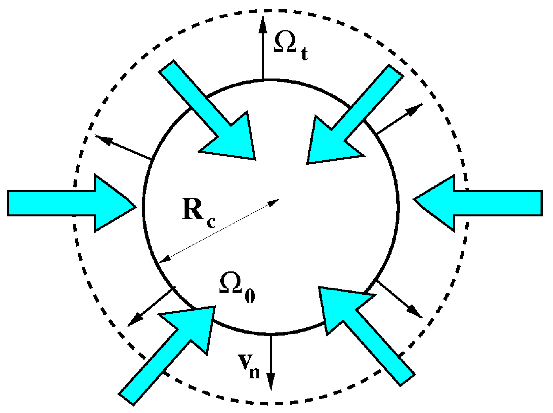
Figure 2.
Schematic representation of the structure of the cell membrane. AQP: aquaporin (cyan). The ion channel is drawn in green. Water molecules (red and dark blue), charged solutes (magenta) and neutral solutes (brown) are illustrated. The lipid constituent is drawn in yellow. The AQP is selective to water molecules whereas the ion channel permits the co-transport of ions and water.
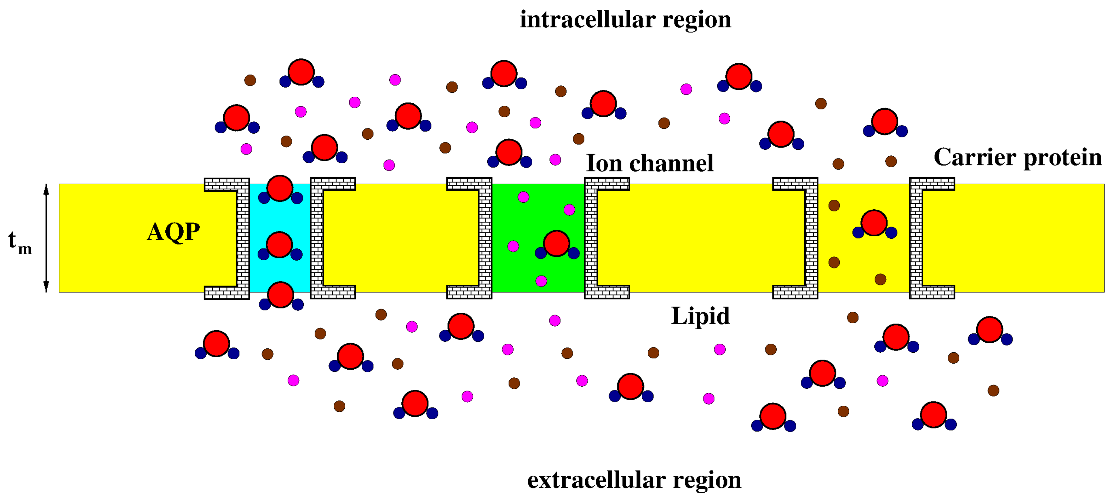
Figure 3.
Three-dimensional schematic representation of an aquaporin. The cylindrical domain is the pore channel, is the membrane thickness and is the aquaporin radius.
Figure 3.
Three-dimensional schematic representation of an aquaporin. The cylindrical domain is the pore channel, is the membrane thickness and is the aquaporin radius.
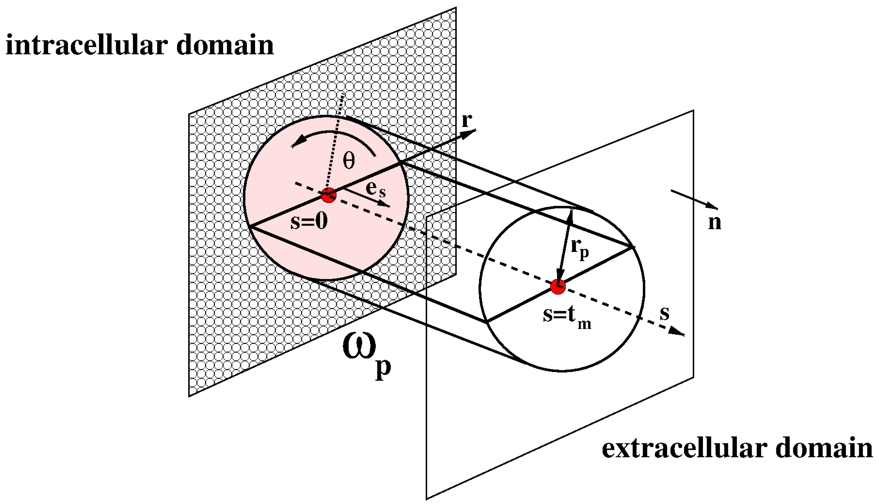
Figure 4.
Transmembrane electric potential.
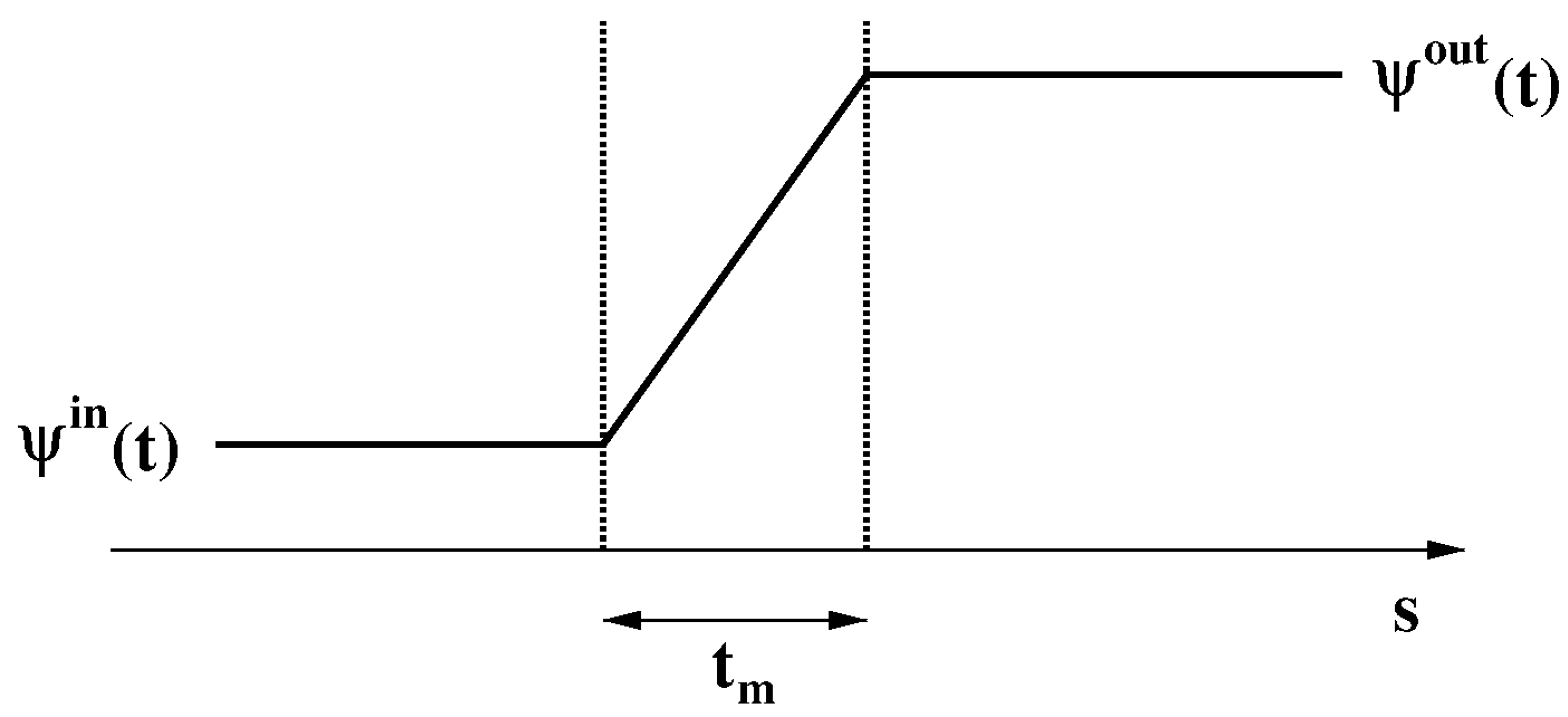
Figure 5.
Left panel: plot of . Right panel: plot of in the time interval . The values of the input data are: , , , and . Right panel:
Figure 5.
Left panel: plot of . Right panel: plot of in the time interval . The values of the input data are: , , , and . Right panel:
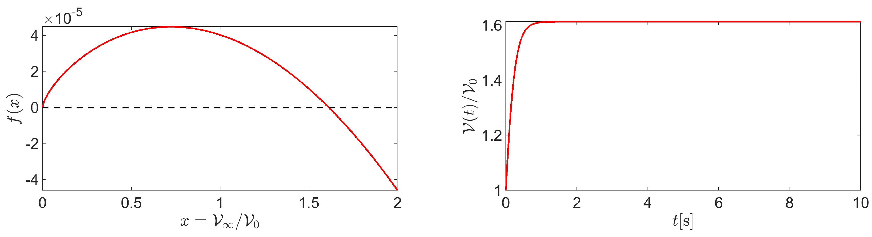
Figure 6.
Left panel: plot of in the time interval . Fluid velocity varies in the range . The arrow indicates velocity increase from negative to positive values. Right panel: plot of in the time interval .
Figure 6.
Left panel: plot of in the time interval . Fluid velocity varies in the range . The arrow indicates velocity increase from negative to positive values. Right panel: plot of in the time interval .
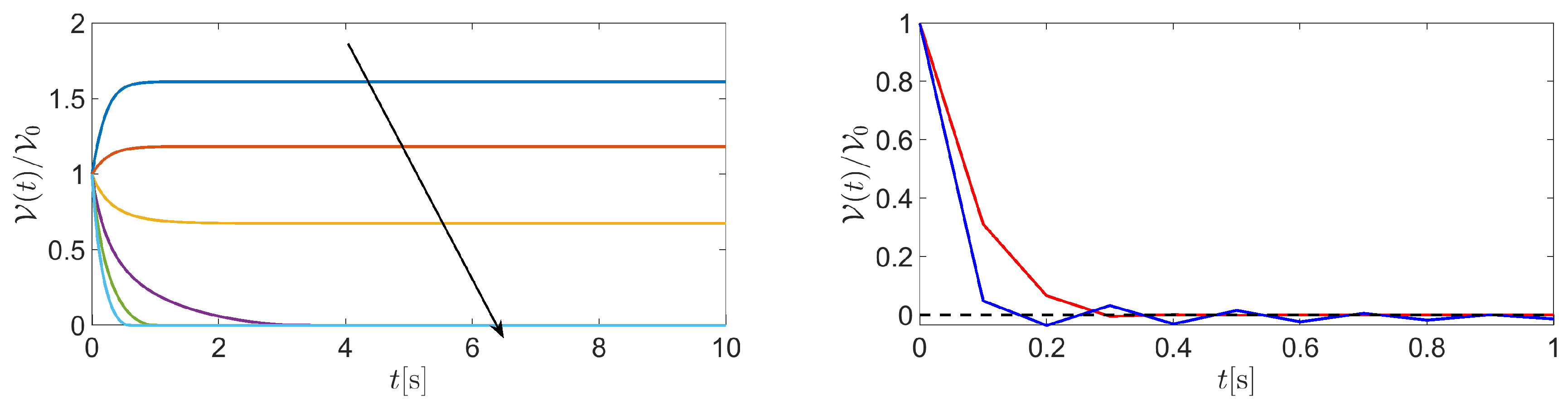
Figure 7.
Left panel: plot of the water volume net production rate in the time interval . Right panel: plot of in the time interval in the case where for every . Fluid velocity varies in the range . The arrow indicates velocity increase from negative to positive values.
Figure 7.
Left panel: plot of the water volume net production rate in the time interval . Right panel: plot of in the time interval in the case where for every . Fluid velocity varies in the range . The arrow indicates velocity increase from negative to positive values.
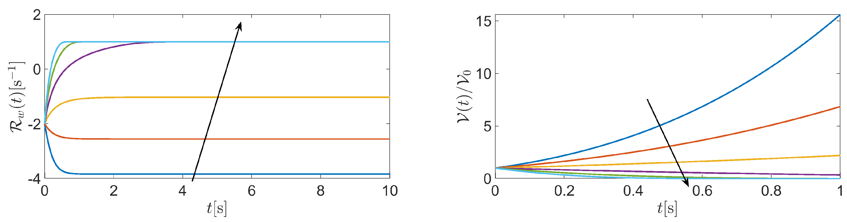
Figure 8.
Left panel: blue curve: , red curve: , . Right panel: blue curve: , red curve: , . Middle panel (bottom): total AH volumetric flow rate for .
Figure 8.
Left panel: blue curve: , red curve: , . Right panel: blue curve: , red curve: , . Middle panel (bottom): total AH volumetric flow rate for .
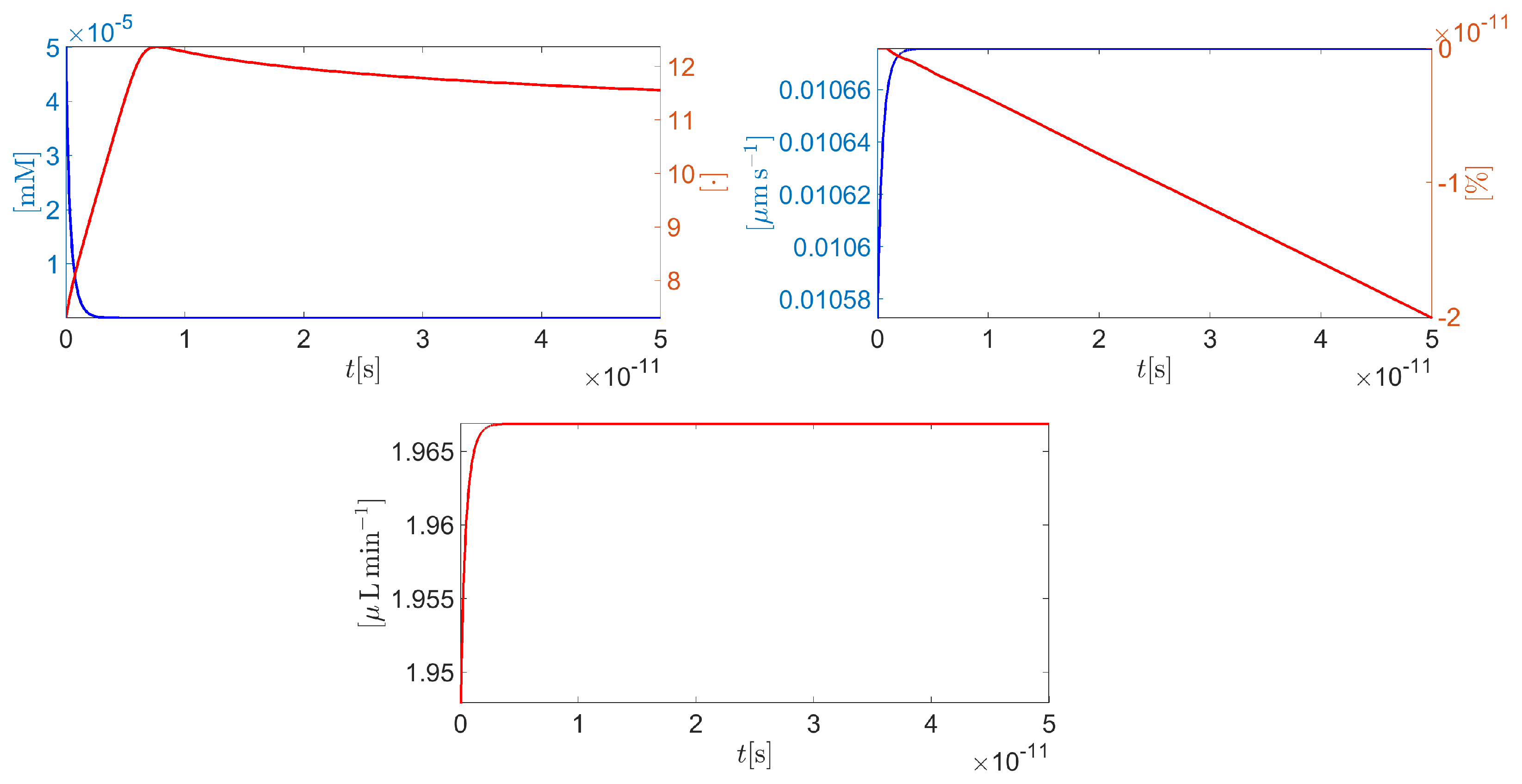
Figure 9.
Top left panel: blue curve: , red curve: , . Top right panel: blue curve: , red curve: , . Bottom left panel: blue curve: average cell normal surface velocity , red curve: percentage volume variation , . Bottom right panel: total AH volumetric flow rate for .
Figure 9.
Top left panel: blue curve: , red curve: , . Top right panel: blue curve: , red curve: , . Bottom left panel: blue curve: average cell normal surface velocity , red curve: percentage volume variation , . Bottom right panel: total AH volumetric flow rate for .
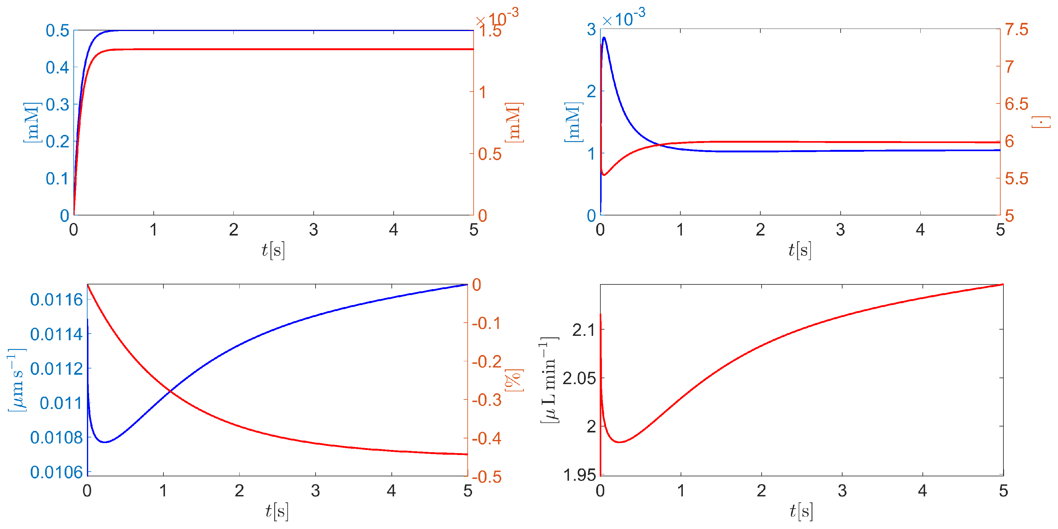
Figure 10.
Top left panel: zoom of the membrane potential (units: ) in the time interval . Top right panel: zoom of (blue curve); (red curve); (green curve) (units: ) in the time interval . Middle left panel: zoom of chlorine molar flux density (units: ) in the time interval . Middle right panel: zoom of (blue curve); (red curve) in the time interval . Bottom center panel: zoom of the total AH volumetric flow rate in the time interval .
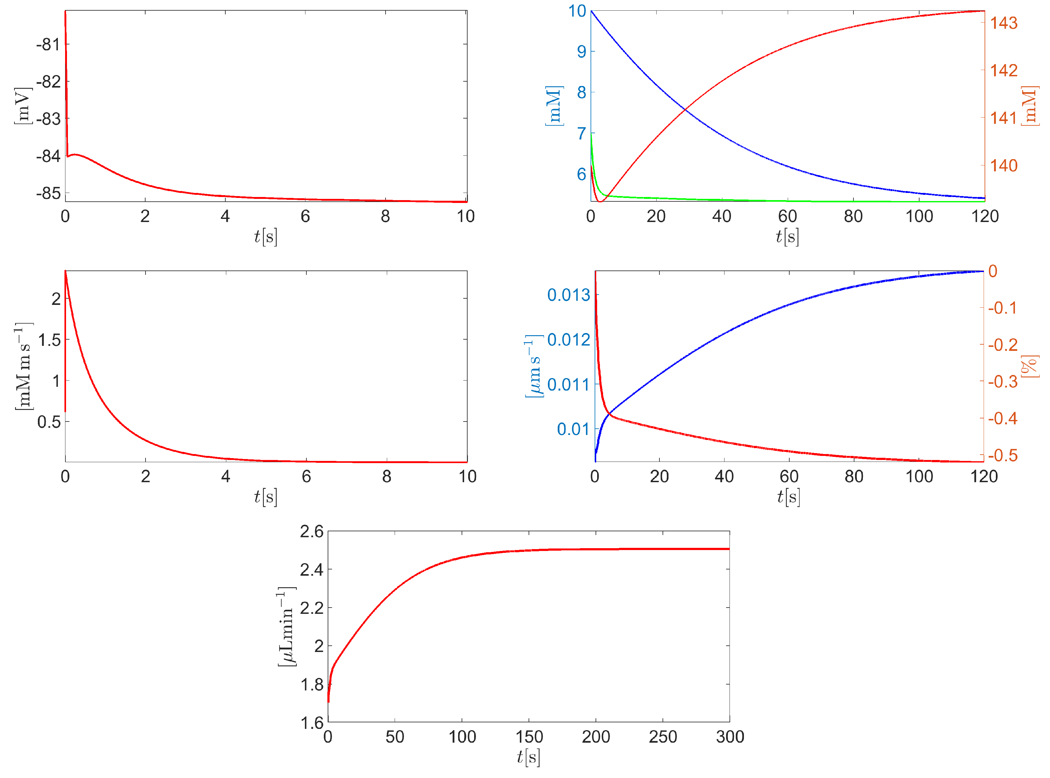
Figure 11.
Schematic representation of the processes involved in AH dynamics. (1): AH production; (2): AH flow; (3): AH outflow. Reprinted from R. Ramakrishnan et al, Diagnosis & Management of Glaucoma, Chapter 9 Aqueous Humor Dynamics, 10.5005/jp/books/11801_9, (2013) [34]; used in accordance with the Creative Commons Attribution (CC BY) license.
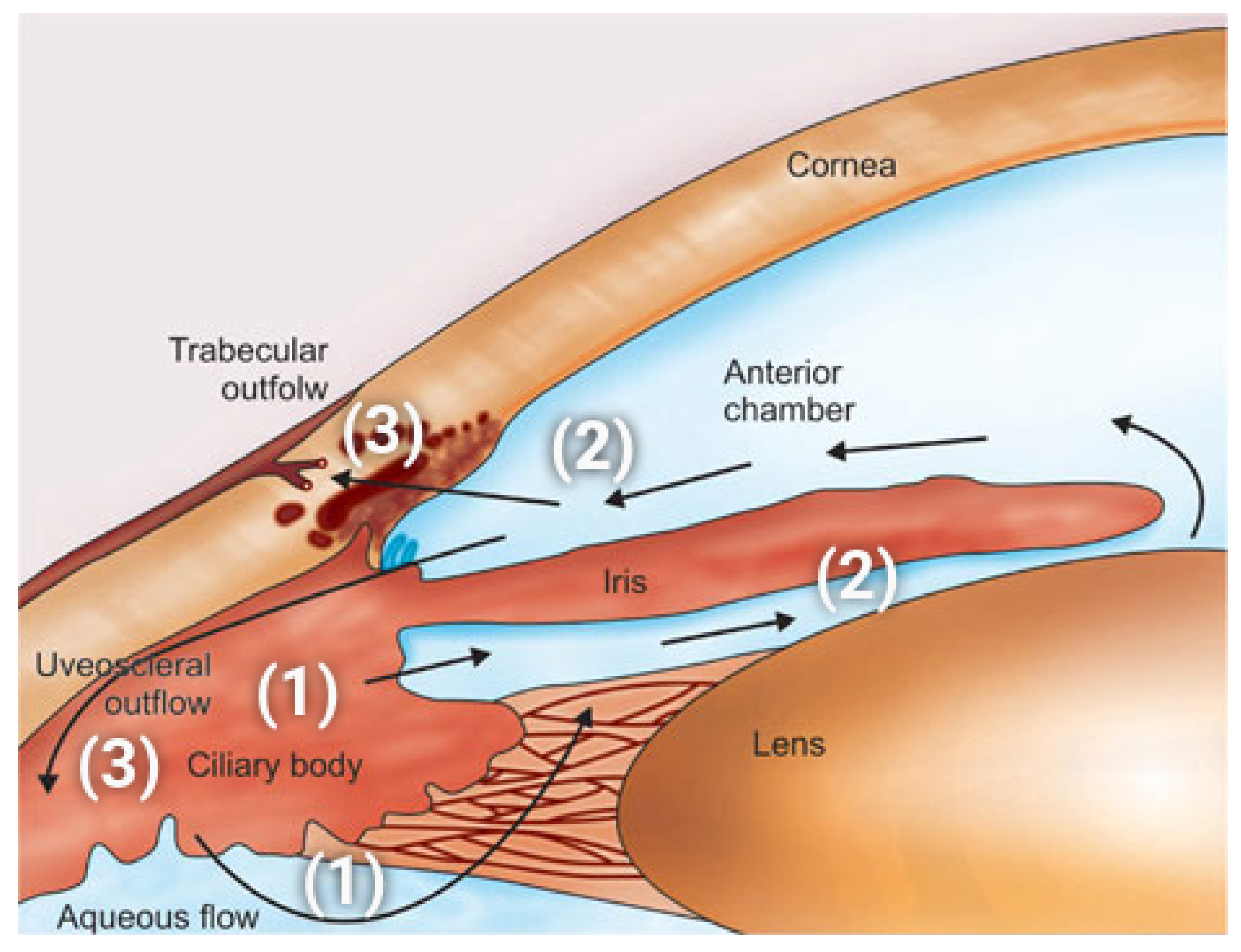
Figure 12.
Left panel: total AH volumetric flow rate for as a function of . The black dashed line indicates the physiological value of , equal to 2.75 , when IOP = 15 mmHg. Right panel: total osmo-oncotic pressure difference for as a function of .
Figure 12.
Left panel: total AH volumetric flow rate for as a function of . The black dashed line indicates the physiological value of , equal to 2.75 , when IOP = 15 mmHg. Right panel: total osmo-oncotic pressure difference for as a function of .
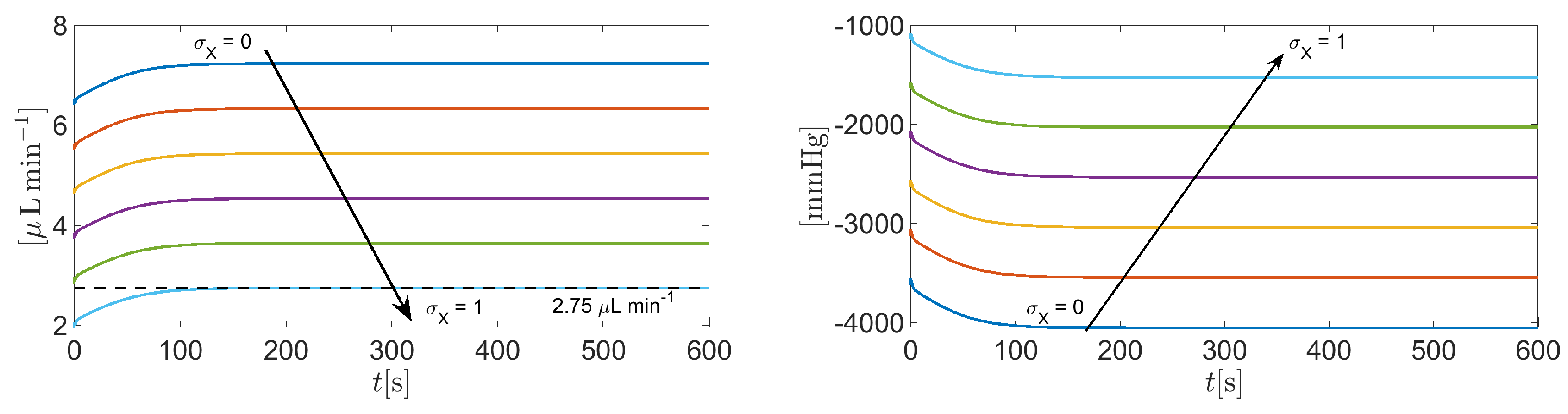
Figure 13.
Total AH volumetric flow rate for as a function of . The black dashed line indicates the physiological value of , equal to 2.75 , when IOP = 15 mmHg.
Figure 13.
Total AH volumetric flow rate for as a function of . The black dashed line indicates the physiological value of , equal to 2.75 , when IOP = 15 mmHg.
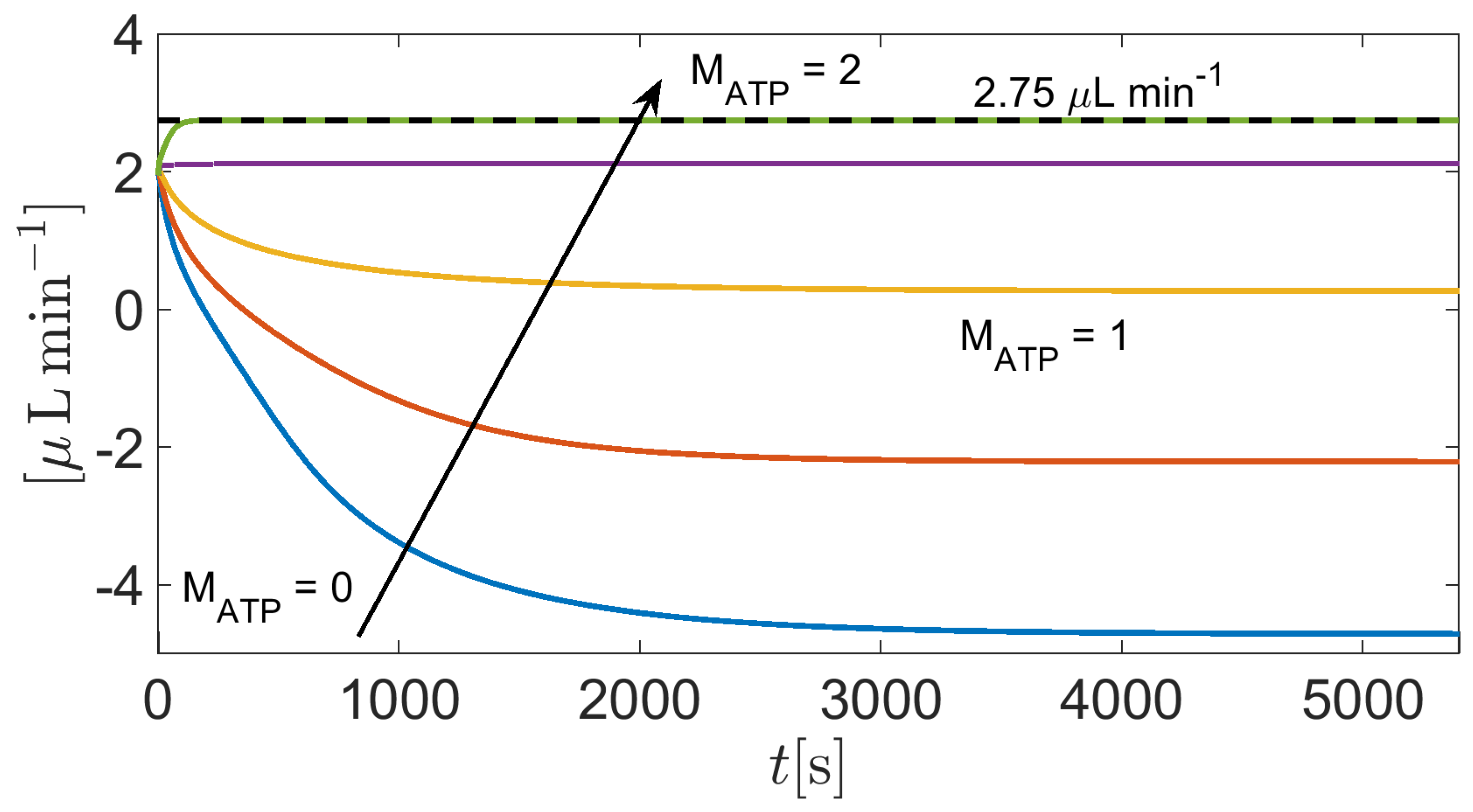
Figure 14.
Zoomed view of total AH volumetric flow rate for as a function of . The physiological value of is equal to 2.75 when IOP = 15 mmHg.
Figure 14.
Zoomed view of total AH volumetric flow rate for as a function of . The physiological value of is equal to 2.75 when IOP = 15 mmHg.
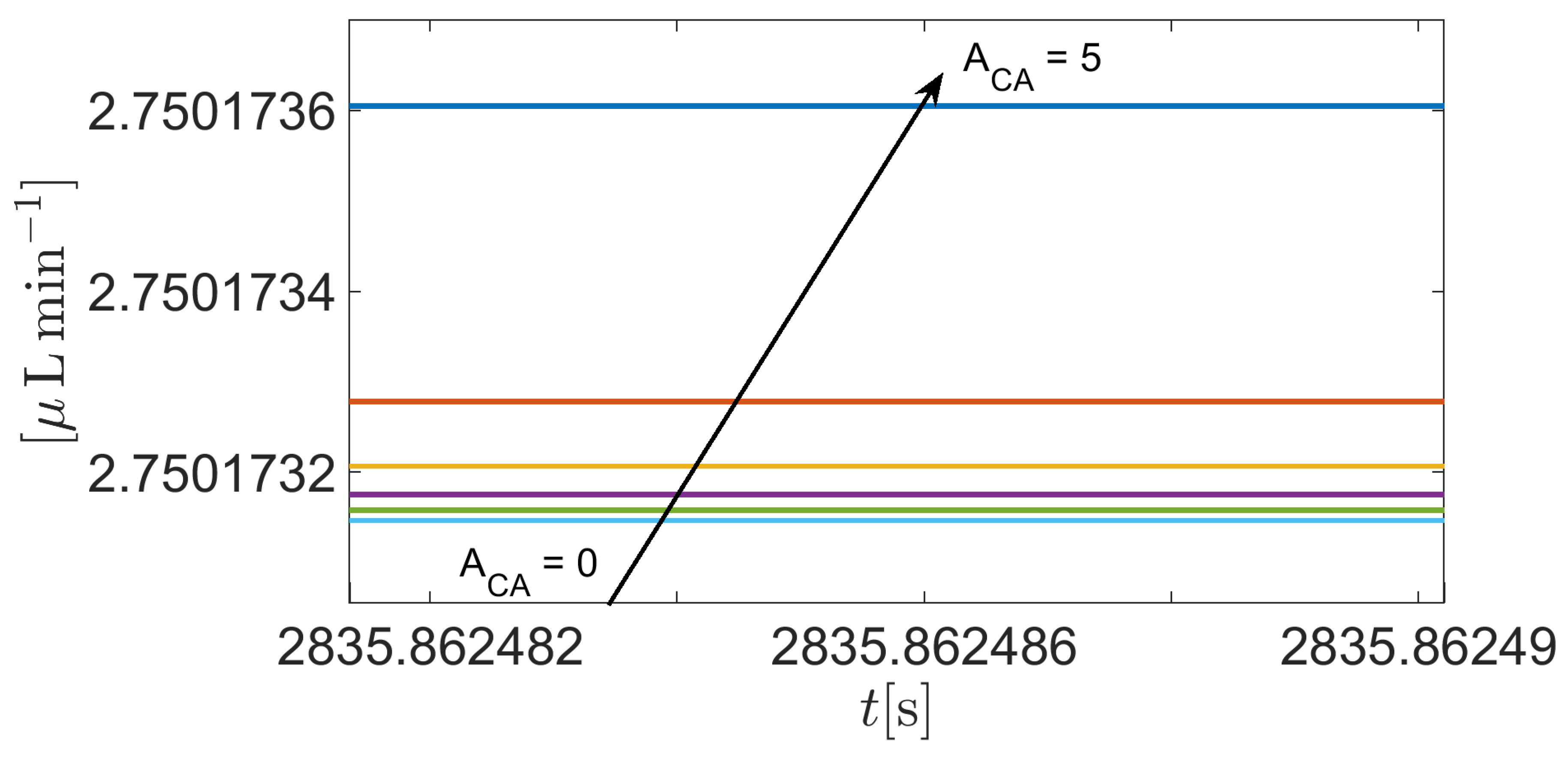
Figure 15.
Plot of the % difference between at baseline conditions and for IOP in the interval [15, 150] mmHg, with .
Figure 15.
Plot of the % difference between at baseline conditions and for IOP in the interval [15, 150] mmHg, with .
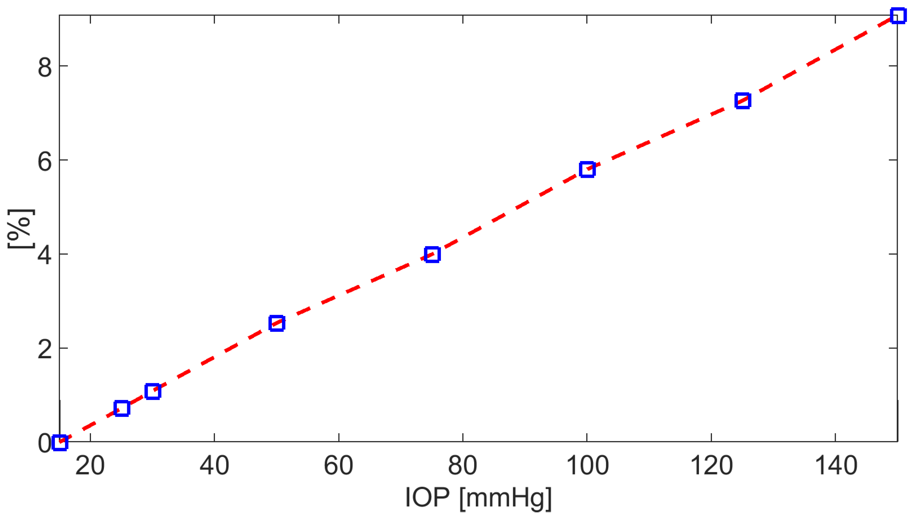

Table 1.
Model parameters: symbol, value and units.
| Symbol | Value | Units |
|---|---|---|
| T | 298.15 | K |
| m | ||
| m | ||
| 1 | ||
| 0.9974 |
Disclaimer/Publisher’s Note: The statements, opinions and data contained in all publications are solely those of the individual author(s) and contributor(s) and not of MDPI and/or the editor(s). MDPI and/or the editor(s) disclaim responsibility for any injury to people or property resulting from any ideas, methods, instructions or products referred to in the content. |
© 2024 by the authors. Licensee MDPI, Basel, Switzerland. This article is an open access article distributed under the terms and conditions of the Creative Commons Attribution (CC BY) license (https://creativecommons.org/licenses/by/4.0/).
Copyright: This open access article is published under a Creative Commons CC BY 4.0 license, which permit the free download, distribution, and reuse, provided that the author and preprint are cited in any reuse.


