Preprint
Article

This version is not peer-reviewed.

Enhancing Risk Assessment with Generative Models

Submitted:

18 December 2024

Posted:

19 December 2024

Read the latest preprint version here

Abstract

Conditional Value-at-Risk (CVaR) is one of the most popular risk measures in finance, used in risk management as a complementary measure to Value-at-Risk (VaR). VaR estimates potential losses within a given confidence level, such as 95% or 99%, but does not account for tail risks. CVaR addresses this gap by calculating the expected losses exceeding the VaR threshold, providing a more comprehensive risk assessment for extreme events. This research explores the application of Denoising Diffusion Probabilistic Models (DDPM) to enhance CVaR calculations. Traditional CVaR methods often fail to capture tail events accurately, whereas DDPMs generate a wider range of market scenarios, improving the estimation of extreme risks. However, these models require significant computational resources and may present interpretability challenges.

Keywords: 
;  ;  ;  ;  ;  ;  

Introduction

Risk management one of the most importance concept in finance. In the world was a lot of crisis event like Worldwide crisis in 2008 and Covid-19 in 2020, so forced financial regulators to more effectively assess risks for investors, to be ready to sudden capital shortfalls. From that time in financial world started to develop some of mechanism that requires financial instruments to calculate risk measures. One of the common risk measure is Value-at-Risk(VaR). Value-at-Risk is the measure that calculates the overall losses in some of evidence level over a certain period of time, it is good for understanding the losses in some level of evidence, like 95% or 99%, but Value-at-Risk cannot to calculate Tail Risks. Conditional Value-at-Risk is additional to the Value-at-Risk, because it is precisely this that can take Tail Risks into account. This is important because events that being rarely have strong impact to the market. Value-at-Risk and Conditional Value-at-Risk became popular in 2004, after the Introduction of the Basel II Accord, recommendations for banks which relied on the VaR to determine capital for market risk protecting.
The part of VaR and CVaR is the correctly loss distribution. The main goal of these measures is predicting financial losses using conservative approaches, but market data poses many features, that cannot to analyze with simple distributions.
The traditional method of calculating CVaR is Sample Average Approximation(SAA). SAA is based on using historical or new simulative data for valuation of distribution of asset return. Function of SAA is minimize CVaR in some of limitations. The traditional method involves that data of profitability and equally distributed, it means the traditional method cannot be always correct in finance market.
Some archives in Deep Learning that opening some of types of models as Generative Adversarial Networks(GANs), Variational Autoencoders(VAEs), Deep Generative Models(DGM), Denoising Diffusion Probabilistic Models(DDPM). These models opens a opportunity for new methods to calculate VaR and CVaR. Generative Models can simulate new samples of asset’s profit based on historical data of assets. It is useful for CVaR calculating, because that need to understanding of Tail Risks, which may be badly covered by traditional models. Finance returns often demonstrate not normal characteristic as asymmetric and heavy tail, but Generative Models can better to capture these complex behaviors, which allows you to assess risks more accurately. Also Generative Models could analyze more data, because that can effectively minimize size of data, that do calculating of CVaR easily in high-quality of data. Providing more accurate assessment of Tail Risks, Generative Models improve manager’s ability to do correctly answers. It helps to provide better strategies risk reduction and improved portfolio optimization.
The difference between Denoising Diffusion Probabilistic Models and others in that the DDPM have more advantages in generation of data, especially in hard tasks. DDPM can more correctly modeling complex data distributions, it is critical for finance markets with heavy tails and not stable patterns. The DDPM in contrast to GANs can provide more stable learning process, it helps to avoid problems with setting and teaching a model. Also DDPM adapted to work with time series that do it especially useful for finance data where important to take into account time and dynamic of the finance portfolio.
The main goal of this research that prove that the DDPM is more suitable model for CVaR calculating, that could improve accuracy of CVaR to avoid making decisions that could negatively impact the company's financial profile.

Definition of VaR and CVaR

One of the most hardest task in financial risk management is measurement and control potential losses. VaR and CVaR are the most popular risk measures in the financial risk management. VaR is the maximal loss, that portfolio could lose with limited probability, CVaR is expected loss.
For example from Yamai and Yoshiba (2005) in their critique of VaR's inability to account for tail losses [3]: If portfolio is 1 mil$, my confidence level is 95% and if my VaR on 95% level for 1 day equal 50.000$, that means with probability of 95% my portfolio will no lose more than 50.000$, but with the remaining 5% chance, losses could exceed 50.000$.
CVaR is improved version of VaR, that analyzes losses, which exceeding VaR value. So, CVaR shows average losses in 5% of confidence level.
For example:
  • VaR on 95% of confidence level = 50.000$
  • CVaR on 95% of confidence level = 70.000$
That means if my portfolio will lose more than 50.000$(event in that 5%), so average loss will be 70.000$.
This risk measures uses banks and funds to assess the daily risk of their assets. But CVaR have advantage that CVaR could consider not only big losses probability, but also their average, that makes it more informative for risk assessment in extreme situations.
Aspect Value-at-Risk(VaR) Conditional-Value-at-Risk(CVaR)
Definition Maximum loss at a specific confidence level. Average loss when VaR exceeding.
InformationalValue General understanding of risk, but without what is happening beyond VaR. Helps to understand how serious could be rare and extremal losses.

Traditional Method of CVAR Assessment

  • Historical modelling: using data for previous profit for example for year or other period. Firstly calculating VaR, then only cases where losses exceed the VaR value are considered. CVaR is the average value that losses. For example: If the worst 5% of losses 10.000$, 12.000$, 15.000$ etc., so CVaR is average of that values.
  • Variance-Covariance Method is easy to use and assume that returns follow a normal distribution. After calculating VaR need to average exceeded losses. This method is simple, but its have some limits like poor perform in extreme values in the data.
  • Monte Carlo Simulation: simulating thousands of random scenarios for returns using mathematical models. This method more precise because it can account for non-standard return distributions
No one of this method could not working good with rare, but extreme events.

Definition of Denoising Diffusion Probabilistic Models

DDPM is the type of Generative Models which is designed to learn complex data distribution by adding and removing noise. This model is good works with tasks, where need to modeling complex data, as creating images, text or forecast crisis events.
Model take a data and gradually adds a noise by step, changing the data to the random data(noise). Model is learning "to unfold" that process: It step by step removing noise and restore initial data. This allows the model generate new data, starting from clear noise and change it it to realistic examples.
DDPM using in finance for creating new market scenarios, also rare and extreme situations. It helps better calculate values, like CVaR, because model can takes into events, which traditional methods can skip.
This model is useful tool for forecasting and risk management, especially need to consider rare, but important events.

Advantage of Using Denoising Diffusion Probabilistic Models

Denoising Diffusion Probabilistic Models is different than other Generative Models due to it is unique characteristics that do DDPM more useful for CVaR calculating and modelling tail risks.
  • Accuracy of modelling complex distributions.
    • To evaluate CVaR critical important consider rare, extremal events, that creates “tails” of distributions of losses.
    • DDPM gradually add some noise to the data, that change it to random noise, then learn to delete it and restore the data. It helps to models better learn complex data dependencies.
2.
Generating different market scenarios.
  • For calculating CVaR need create a purge number of possible scenarios, also rare events, that can not be introduced in historical data.
  • After learning DDPM can generate synthetic data, that did not presented in historical data.
3.
Stable of the learning.
  • Generative models as GANs can be non-stable while learning, which leads to problems such as “model collapse”. DDPM uses a sequential learning process that makes learning more stable and less prone to failure.
4.
Interpretability of the Data Structure.
  • Understanding risk requires that the model provides realistic scenarios based on known characteristics of the data. Process of adding and removing noise in DDPM is closely linked to real data, allowing the model to generate plausible market scenarios.
5.
Difference between other models.
  • Unlike other models as GAN and VAE, DDPM better modelling tails of the distributions and less prone to learning problems.
  • DDPM generate high quality data, because it does not simplify the structure of hidden factors within the model.
  • DDPM is easier to scale for complex data, such as time series.
6.
Using DDPM in CVaR calculating
  • CVaR need goof understanding of tail risks, which meet not often in real data.
  • Model can better modeling tail events, improving calculate average loss in the most extreme events.

Disadvantages of Using Denoising Diffusion Probabilistic Models

While DDPM have a lot of advantages in modeling complex distributions and generating realistic data, but DDPM have also some limitations. This limitations can impact to the practice using and effectiveness, especially in finance aspect.
  • Requires significant computational resources:
    • DDPM is resource-intensive due to its multi-step process. This issue can be mitigated by optimizing the model and utilizing advanced hardware.
2.
Challenges in interpreting outcomes:
  • Understanding the results of generative models can be difficult. However, visualizing the scenarios produced by DDPM helps make the analysis more intuitive.

Methodology

The research methodology centers around the implementation and evaluation of a Denoising Diffusion Probabilistic Model (DDPM) to calculate Conditional Value-at-Risk (CVaR) for financial datasets. The steps involved in the methodology are as follows:
  • Data Preprocessing:
    The dataset used comprises daily returns of financial instruments from the S&P 500 index. The data includes timestamps, asset names, and their respective returns.
    Missing data points are handled using imputation techniques, and returns are calculated from adjusted closing prices.
    Data normalization is performed to ensure that all inputs lie within a consistent scale, aiding the stability of the model during training.
2.
Model Architecture:
The DDPM consists of a neural network that learns to model the noise distribution applied to the data during the forward diffusion process. The network architecture includes multiple convolutional layers to capture both temporal dependencies and high-dimensional features.
Key components include:
Encoder-Decoder Framework: Encodes input data into a compressed latent representation and decodes it during the reverse process.
Attention Mechanisms: Incorporated to focus on key temporal patterns in the data.
Noise Scheduler: Determines the magnitude of noise added at each timestep.
3.
Training Process:
The forward diffusion process involves adding Gaussian noise to the data iteratively, controlled by the noise schedule.
The reverse diffusion process learns to denoise the data by predicting the added noise at each timestep.
A loss function, typically Mean Squared Error (MSE), measures the difference between the predicted and actual noise at each step.
The model is trained over multiple epochs using the Adam optimizer, with learning rate decay to stabilize convergence.
4.
CVaR Calculation:
Synthetic return scenarios are generated using the trained DDPM. These scenarios include rare and extreme events that traditional methods often miss.
VaR is calculated at the desired confidence level (e.g., 95%).
CVaR is derived by averaging the losses that exceed the VaR threshold across the generated scenarios.
5.
Model Evaluation:
The DDPM's performance is compared against traditional methods such as Historical Simulation and Monte Carlo Simulation.
Evaluation metrics include:
Accuracy: Ability to replicate historical tail risks.
Robustness: Performance under volatile market conditions.
Computational Efficiency: Time and resources required for training and inference.

Application of Denoising Diffusion Probabilistic Models (DDPMs)

DDPMs are a class of generative models that learn complex data distributions by iteratively adding and removing noise. This process allows DDPMs to generate realistic synthetic data, which is valuable for CVaR estimation as it captures tail events often missed by traditional methods.
DDPMs operate in two primary phases:
  • Forward Process: In this phase, noise is gradually added to the data over several timesteps. This transforms the original data into a completely noisy representation. The forward process is defined by a noise schedule that determines how noise is incrementally added. This phase ensures that the data becomes independent of its original distribution, preparing it for unbiased generation during the reverse process.
  • Reverse Process: Once the model learns the noise patterns from the forward process, it begins the reverse process, gradually denoising the data to reconstruct the original distribution. The reverse process is guided by a trained neural network that predicts the noise at each timestep. This step requires sophisticated optimization techniques to ensure accurate reconstruction and meaningful data generation.
By leveraging this two-phase approach, DDPMs excel at capturing the nuances of complex financial datasets, such as heavy tails and asymmetric distributions, which are common in market data. The iterative nature of DDPMs allows for high-resolution modeling, enabling precise representations of rare events and tail risks that traditional methods struggle to quantify.

The Role of Hyperparameters in DDPMs

The performance of DDPMs heavily depends on several hyperparameters, including the noise schedule, the number of timesteps, and the architecture of the underlying neural network. The noise schedule, in particular, determines how aggressively noise is added during the forward process, influencing the model's ability to capture fine-grained details. Balancing these hyperparameters is critical for achieving optimal results, as overly aggressive noise schedules can lead to loss of information, while conservative schedules may result in insufficient generalization.

Comparison with Traditional Models

Unlike traditional methods such as Historical Simulation or Monte Carlo, DDPMs do not rely on fixed assumptions about the underlying data distribution. This flexibility allows DDPMs to adapt to non-normal distributions and incorporate temporal dynamics. Moreover, while Monte Carlo simulations require extensive computational resources to generate numerous scenarios, DDPMs achieve comparable or superior results with fewer iterations by learning the data distribution directly.
Advantages of DDPMs:
  • Accurate Tail Risk Modeling: DDPMs effectively capture rare and extreme events, enhancing the accuracy of CVaR calculations.
  • Synthetic Scenario Generation: By generating diverse market scenarios, DDPMs improve risk assessment under extreme conditions.
  • Stability: Unlike GANs, DDPMs offer a more stable training process, reducing the risk of model collapse.
  • Time-Series Adaptability: DDPMs are well-suited for financial data, incorporating temporal dynamics into risk modeling.
  • High Resolution: The iterative process enables DDPMs to generate detailed and realistic scenarios, critical for tail risk analysis.
  • Challenges of DDPMs:
  • Computational Resources: The iterative process of DDPMs requires significant computational power, as it involves multiple forward and reverse steps for each data sample.
  • Interpretability: Understanding the outcomes of generative models can be complex, although visualizing generated scenarios aids analysis.
  • Hyperparameter Sensitivity: Achieving optimal performance requires careful tuning of noise schedules and model architecture.
Key Graphs and Descriptions
  • Daily Returns During COVID-19
Description: The graph illustrates the daily returns of AAPL, GOOG, and AMZN stocks during the COVID-19 period. High volatility is observed in the initial months, stabilizing over time. This highlights the need for robust risk measures like CVaR to handle extreme fluctuations.
Preprints 143394 g001
2.
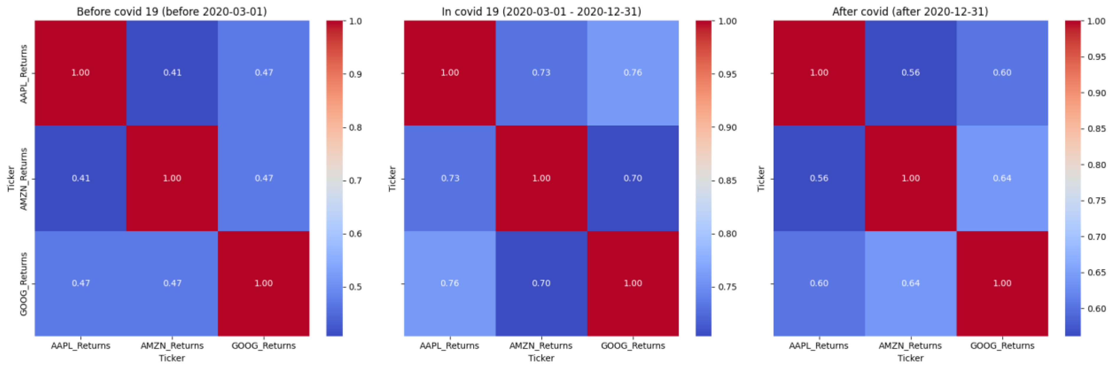
Correlation Heatmaps Across Periods
Description: The heatmaps compare stock return correlations before, during, and after the COVID-19 pandemic. During the pandemic, correlations increase significantly, indicating synchronized movements in the market. This underscores the importance of accurate tail risk modeling.
Preprints 143394 g002
3.
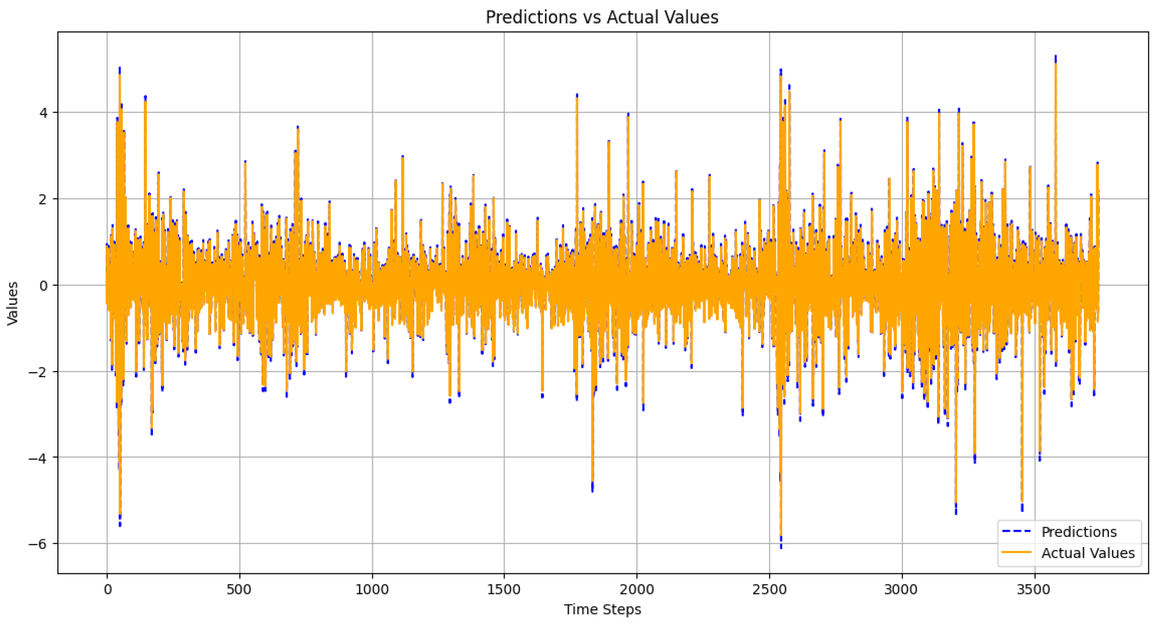
Prediction vs. Actual Values
Description: This graph compares model predictions with actual values, showing a strong alignment under stable conditions. Deviations at extreme peaks highlight areas for further model optimization.
Preprints 143394 g003
4.
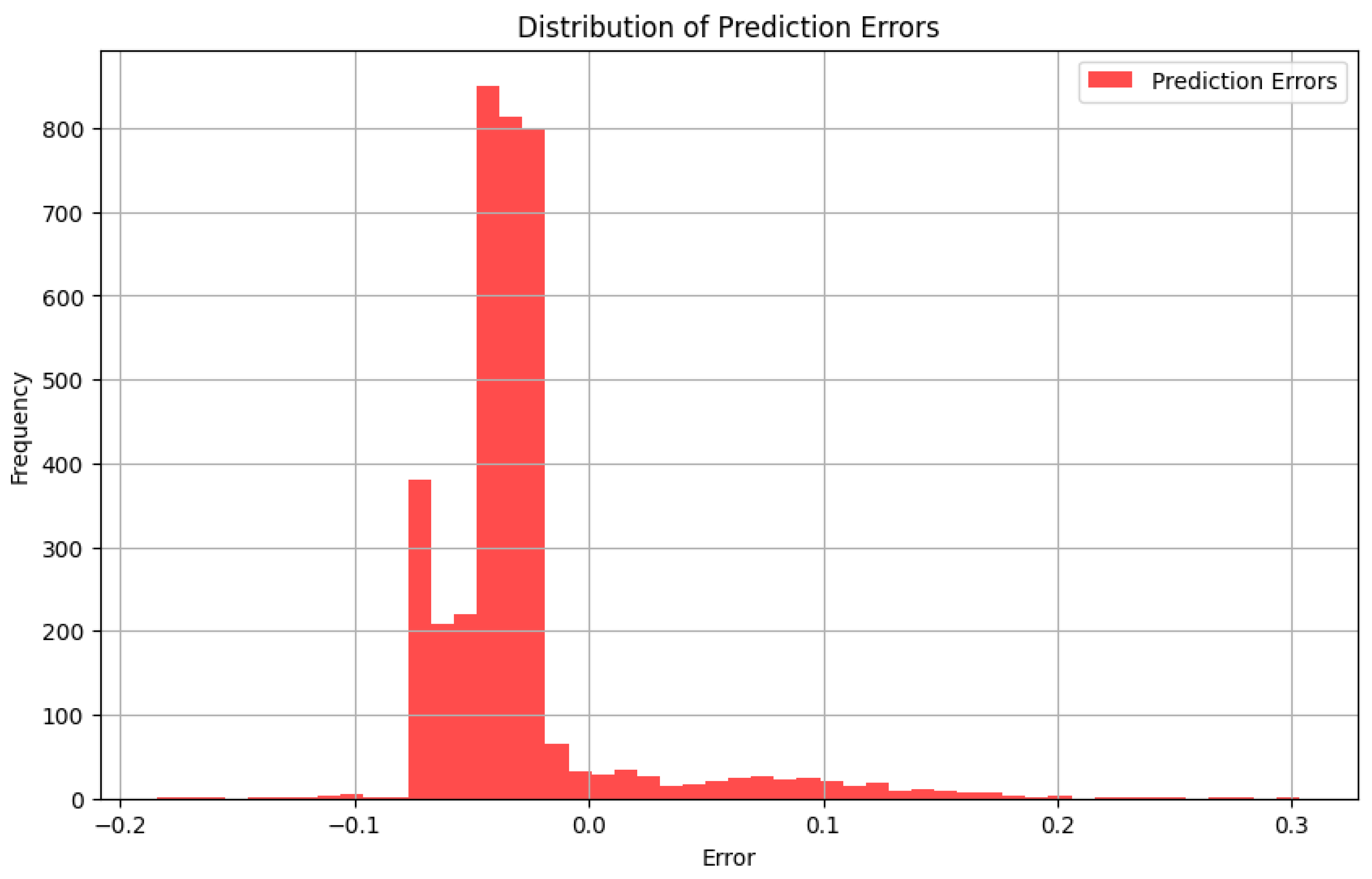
Error Distribution Histogram
Description: The histogram displays prediction errors, mostly concentrated around zero, confirming the model’s accuracy. Larger errors represent rare or challenging scenarios.
Preprints 143394 g004

Conclusion

This research demonstrates the potential of Denoising Diffusion Probabilistic Models (DDPMs) in enhancing Conditional Value-at-Risk (CVaR) calculations. By accurately modeling tail risks and generating synthetic data, DDPMs provide a robust tool for financial risk assessment. Despite challenges such as computational demands and interpretability, the benefits of DDPMs in addressing the limitations of traditional methods make them a promising approach for modern risk management frameworks. Future research should focus on optimizing hyperparameter tuning and exploring the integration of DDPMs with hybrid modeling techniques to further enhance their practical applicability.

References

  1. Yamai, Y.; Yoshiba, T. Value-at-Risk versus Expected Shortfall: A Practical Perspective. Journal of Banking & Finance 2005, 29, 997–1015. [Google Scholar]
  2. Rockafellar, R.T.; Uryasev, S. Optimization of Conditional Value-at-Risk. Journal of Risk 2000, 2, 21–41. [Google Scholar] [CrossRef]
  3. Goodfellow, I.; et al. Generative Adversarial Networks. arXiv 2014, arXiv:1406.2661. [Google Scholar] [CrossRef]
  4. Kingma, D.P.; Welling, M. Auto-Encoding Variational Bayes. arXiv 2014, arXiv:1312.6114. [Google Scholar]
  5. Ho, J.; et al. Denoising Diffusion Probabilistic Models. Advances in Neural Information Processing Systems 2020, 33, 6840–6851. [Google Scholar]
Disclaimer/Publisher’s Note: The statements, opinions and data contained in all publications are solely those of the individual author(s) and contributor(s) and not of MDPI and/or the editor(s). MDPI and/or the editor(s) disclaim responsibility for any injury to people or property resulting from any ideas, methods, instructions or products referred to in the content.
Copyright: This open access article is published under a Creative Commons CC BY 4.0 license, which permit the free download, distribution, and reuse, provided that the author and preprint are cited in any reuse.
Prerpints.org logo

Preprints.org is a free preprint server supported by MDPI in Basel, Switzerland.

Subscribe

Disclaimer

Terms of Use

Privacy Policy

Privacy Settings

© 2026 MDPI (Basel, Switzerland) unless otherwise stated