Submitted:
18 December 2024
Posted:
18 December 2024
You are already at the latest version
Abstract
We investigate the circle design in bubble chart in this paper. The bubble chart we design has the properties that a unit circle is at the center, and surround by a series of circle rings one layer by one layer. For extending next layer of circles, it always has a silhouette circle tangent to all circles in the newest layer. The extension of circle is partition into two class, one is that each layer has the same number of circles with the same radii, the other is that new layer has multiple numbers of circles, compare with the previous layer of circles. We solve the problem geometrically and/or algebraically if the problem is simple, and give heuristic algorithm to solve more complex problem.
Keywords:
circle packing
; word cloud
; computer-aided geometric design (CAGD)
; geometric constraint solver (GCS)
MSC: 65D18
1. Introduction
The circle play an import role in history, and used in many different filed such as geometry, engineering, mechanics, architecture design, art design. Many researches tried to find properties for circle [1,2], so that properties of the circle can be used in the application properly. In infographics, circles are commonly used in data visualization[3], such as in pie charts, bubble charts[4,5], donut chart, circular treemaps, radial bar chart, chord diagram, to convey categorical or quantitative data in visually effective way. The bubble chart use bubble, represented by a circle, whose center and radius can represent at least 3 dimensional data. For example, a manufacture company want its product a bubble chart, so that x represents the product categories, y represents average sales price, and r represents the total unit sold. These circles can combine with other chart. Heer, J., Bostock, M., & Ogievetsky, V. (2010) [6](See Figure 1), the geospatial data combine with pie chart, it shows the percentage of the obese, normal, overweight percentage, represent by a pie chart, in every states. In this case, (x,y) position is not so import, as long as it location is inside the associated state, the size of circle represents the total population. In Figure 1(a), 5 dimensional data are represented, include state categories and obese, normal, overweight, total population in each state. If we want know only the percentage of the overweight population, the pie chart in Figure 1(a) can be replaced by a circle whose size represents the percentage of the overweight population, as show in Figure 1(b). In this figure, the designer tried to avoid the overlapping of circles, and did not ask tangency properties among circle.
Some researchers give constraints among circle, such as tangent internally/externally. For example, Wang, W., Wang, H., Dai, G., & Wang, H. (2006) [7](see Figure 2) want to see the tree structure for file system using nested circles. The circles tangent externally means this two are represented at the same level (brother relationship). The circle inside a circle means that these two circles are in different level (father/son relationship). See Figure 2(b). The author also add cylinder in the Figure, the cylinder′s height represents one more dimension of data. For example, the height of the cylinder can represent the size of memory used in this directory. In this figure, the tangency property among circle are used, so to minimize the waste space.
The circle tangency problem has been investigating for many years. For example, the Apollonius problem try to find circles tangent to three circles [8], and the malfatti problem try to find three circles inside a triangle with the properties that each circle tangent to other two circles externally, and also tangent to two sides of the triangle [9]. The circle packing problem [10] try to put non-overlap circles inside an area, such as triangle, square, circle, and find a way to produce many circles inside the area, such that the total area of these circles is maximum [9,11,12,13]. These circles may have some constraints, such as the same radii, or two different radii. To solve these problem, some researcher uses mathematical analysis geometrically or algebraically, and prove the solution is optimal. Some researchers use heuristic algorithms to find the solution. Dckard Specht [14] gives algorithms to find n circles with the same radius inside a unit circle. It finds all solutions with maximum circles area for the case n=1 to 1000, some solutions are optimal, and some solutions are still a conjecture. Notice that for the optimal solution the circles inside the unit circle tangent to other circle often. When this problem allows two different radii for the inside circles, the problem become more complex [15]. The more radii the problem allowed, the more complex the problem is.
To construct circle tangency graph, we need to describe the circle packing theorem [16]:
For every connected simple planar graph G, there is a circle packing in the plane whose intersection graph is (isomorphic to) G. The intersection graph, also called tangency graph, whose vertex represent circle, and edge connecting two vertices represent these two circles tangents to each other.
By this theorem, given a simple planar graph G, we can construct its associated circle packing chart.
There are many different algorithms to construct different circle tangency chart. Collins and Stephenson construct a simple planar graph G, and construct its associated circle tangency chart [16]. For some applications, such as the bubble chart combine with word cloud, it emphasis on the radius of circles and put words inside the circle, and the larger circle contains the words which shows more frequent in a book, in some author’s writing, in a column, etc. This radii for circles in this chart may be different, so that the frequency the word shows is easy to identify. Notice that the circle may/may not tangent to its neighbor circles. For visual effect, the larger circle with word inside, which represents the word written by the author more often, should put on the center of the chart, because the center of the chart get more attention by the reader.
In this research, we would like to find a way to construct bubble chart, so that all of the bubble circle satisfied certain criterion. We start from a unit circle centered at the origin, and extend circles layer by layer, from inside out, so that all circles have tangency properties with one or two circles in previous layer, two circles the same layer, and tangent to a large circle centered at the origin.
Let us classify the bubble chart we want to construct, and these chart associated with the problem we need to solve, including BC[1,n], BC[1,n,n], BC[1,n,n,…,n] and BC[1,n,mn] problem. In these problem, there is always a unit circle in the center, and a silhouette circles tangent to circles at the last layer. The BC[1,n] problem is the problem to generate the first/last layer of n circles, as shown in Figure 3(a) for n=8. The BC[1,n,n] problem has two layers of circles, as shown in Figure 3(b) for n=6. BC[1,n,n,n,…] is the extension of BC[1,n] and BC[1,n,n], it can be construct by more than two layers. The last bubble chart is BC[1,n,mn]. In BC[1,n], the first layers has n circles tangent to the center unit circles, and the second layer has mn circles tangent to the first layer of circles in a special way. Because there is a silhouette circle tangent to the circles at the second layer, there are m different radii of circles at the second layer. The figures for BC[1,6,26] and BC[1,6,36] problem are shown in Figure 3(c)(d) respectively.
In this paper, the closed form for the circles radii in BC[1,n], BC[1,n,n] and algorithms to construct BC[1,mn] are provided.
2. Closed form solution for BC[1,n], and BC[1,n,n]
Before the description for all problems, including BC[1,n] and BC[1,n,n],BC[1,n,.., n],BC[1,n,mn], we would like define some terms. Consider a series of circles C0,C1, C2, …, Cn-1, Ci tangent to Ci-1 and Ci+1 explicitly, i=1, …, n-2, we call these circles a circle chain, as shown in Figure 4(a). When C0 also tangent to Cn-1, we call it a circle ring with size n, as shown in Figure 4(b). We asked the bubble chart we find to solve the associated problem has the property that every circles in the inner layer (all layer except the last layer) has a circle ring around it.
For the BC[1,n] problem, we would like to solve the radii of the circles in a circle ring with size n. The radii for all circles are the same, as shown in Figure 5. It is easy to see that r=, where = . The radius of the silhouette circle whose center is at the origin with radius 1+2r.
For the BC[1,n,n] problem, we need to consider the radius of the circles at the second layer. Consider the case for n=6, as shown in Figure 6(a). Consider figure 6(b), the blue and red circles represent first and second layer of BC[1,n,n] respectively. In figure 6(b), the angle c is equal to the interior angle of a regular convex n-gon, which is (1-)π. Because c+2β+(π-2α)=2π, so β=α+. From cos(α)=, cos(β)==cos(α+)=cos(α)×c-sin(α)×s, where c=cos, s=sin, we can derive c2r22-2(c+s2)r1r2+r12c2=0. There are 2 solutions for this equation, one is the larger radius circle tangent to the first layer and ‘outside’ the layer, and the other small radius is the radius of circle ‘inside’ the layer. So, we find r2=, where c=cos, s=sin. The value can be simplify to . The radius for the silhouette circle will explain when we describe the BC[1,n,…,n].
Notice that we can use the above idea to find the radius of circle ring in the further layer. We can generate a recursive equation rn=Drn-1, r1=, n>1, where D=, s=sin(), c=cos(). Notice that D>1 because ≥1, n>2, so ri≥ri-1. That is, the circles in exterior circle ring has larger radius than the circles in interior circle ring, start from the first circle ring. Notice that is a constant, so we can compute once and find the radius for next layer easily.
We know there is a large silhouette circle tangent to each layer of circles. Assume Ri is the radius of the large silhouette circle, it’s value can be easily computed with the following theorem.
Theorem 1: The radius for the silhouette circle in different layers is:
R0=r0=1
R1=1+2r1
Ri=(Ri-2-ri-2)+f(ri-2,ri-1)+f(ri,ri-1)+ri, where i>1, f(,)=
Proof of Theorem 1. The proof for R0=r0=1, R1=1+2r1 is trivial. Assume f(,) =. This function calculates the distance of the dashed line in Figure 7(a), and consider the value Ri, i>1, Ri can be computed by the sum of 4 values(see Figure 8(b), start from Ri-2-ri-2, and followed by f(ri-2 ,ri-1), f(ri ,ri-1) and ri, so Ri =(Ri-2 -ri-2)+f(ri-2 ,ri-1)+f(ri ,ri-1 )+ri. □
From theorem 1, we have the following corollary:
Corollary 1: The radius of the silhouette circle for n-th layer of circle ring is (center circle is a unit circle):
R0=1; R1=1+2r1; Ri=Ri-2+Di-3()r1, n>2, where r1=, D=, s=sin(), c=cos().
Note that when we know the value n, the value and r1 is a constant. The new value Ri can be computed by a multiplication (D and a computed value) and an addition (with Ri-2). This equation including R2, which is the radius of the silhouette circle for BC[1,n,n] problem.
Now, we can list a table, where n=5,6,7,8,9, and display the radius for the circle at first through sixth layer of BC[1,n,n,n,n,n,n]. We also list the radius of silhouette circle Ri in the Table 1. We can extend the further layer with simple computation.
3. Numerical solution for BC[1, n, m×n]
Consider the BC[1,n], can we extent the chart one more layer (second layer) with 2n circle, and these circles has the same radius? Consider in Figure 8(a), it can be proved that when n=6, we can find the second ring, which has 12 circles, and circles in the first layer tangent to the circles in the second layer in a special way. Furthermore, all the circles have the same radii. Although we can find a silhouette circles for it, it is not the figure we are looking for because the circle in the first layer did not have circle ring around it. Now, consider the case that in Figure 8(b), we want construct BC[1,6,26], the second layer has two different colors of circle, red and green. If these two circles has the same radii, there are two ways to compute the radius of the silhouette circle, one is connecting the line of the center circle to the center of red boundary circle, and find R′=1+2r1,0+2r2,0, where r20 is the radius of red (and green) boundary circle. The other way to compute the radius of the silhouette circle is connecting the line of the center circle to the green boundary circle, and find R=f(1,r1,0)+f(r2,1,r1,0)+r2,1, where f(,)=. After calculation, we find R≠R′。This contradiction tells us that the radii for red and green boundary circles are different.
Now, we want to solve the BC[1,n,2n] algebraically. We need to generate a system of equation, and solve the system of equation via some method such as Newton method. Consider Figure 9, assume Ci(xi,yi,ri) represents a circle Ci, with center (xi, yi) and radius ri. The center unit circle is C0, the circles on the first layer are C1 and C2, we can find all values for Ci(xi,yi,ri), i=0,1,2 when we know the value of n. They are: C0(0,0,1), C1(1+r, 0, r), and C2((1+r)cos(), (1+r)sin()), where r = and = Assume the circles in the second layers are C3, C4, C5, then the variable (xi, yi, ri), i=3,4,5 and the radius for the silhouette circle are the variables. Because the circles C5 is symmetry to the circle C3, with respect to the line passing (0,0) and center of C4, we can find the (x5,y5, r5) values from (x3, y3, r3). So we have 7 variables x4, y4, r4, x5, y5, r5, R, where C(0,0,R) is the silhouette circle. We need to generate 7 equations to find the solution. To generate the system of equation, we need to consider the externally tangency properties, that is, the distance between two circles centers is equal to the sum of their radii. To reduce the number of equations and variables, we try to substitute a variable using other variables, so that the number of equations reduced.
In this case, the circle center can be found from the radius of the silhouette circle. So, (x3,y3)=(R-r3,0)=(1+2r1+r3,0) and (x4,y4)=((R-r4)cos(), (R-r4)sin()). So, x3 is a function with r3 as a variable, y3 is 0, x4, y4 are functions with variables R and r4. We can substitute these 4 variables using other variable in the system of equation, so we need 3 equations only. There are:
C3 tangents to and contains in C: 1+2r1+2r3=R [1]
C4 tangents to C3 explicitly: (x4-x3)2+(y4-y3)2=(r4+r3)2 [2]
C4 tangents to C1 explicitly: (x4-x1)2+(y4-y1)2=(r4+r3)2 [3]
After the substitution of the variable x3, y3, x4, y4, this system of equation becomes:
1+2r+2r3=R [1]
((R-r3)cos()-(1+2r+r3))2+((R-r3)sin())2=(r3+r4)2 [5]
((R-r3)cos()-(1+r))2+((R-r3)sin())2=(r+r4)2 [6]
We know r = and =, this system of equation has 3 variables R, r3, r4. These three equations are degree one, two, two, so it should have 4 solutions.
Now, we can solve this problem numerically using Newton method. However, we did not know what initial value we should guess, so that the solution (r3, r4, R) Newton method find is the real solution we want. The other thing worries us is the system of equation we generate when m>2 become more complex. We need to generate a system of equation for each m value, and the variable for circle center becomes hard to substitute. So we proposed another algorithm to solve this problem.
Before the explanation of the proposed algorithm, we define the SC(C), which is the sum of angle computation for a circle C with the circle ring surround it. Let’s consider three circles C0, C, C1 tangents to each other, and has radii r0, r, r1 respectively. We denote with angle(r0, r, r1) the cosine the angle α between two line segment, one connect the center of C0 and C, and the other connect the center of C and C1, as shown in Figure 10. Notice that angle(r0,r, r1)=cos-1() . This equation can be easily derived from the cosine rule.
Consider a circle ring tangent to one circle, as shown in Figure 11(a), and ri is the radius of Ci. We denote SA(C) is the sum of angle(r0, r, r1), angle(r1, r, r2), …..angle(rn-1,r,r0), which should equal to 2πif the circle ring tangent to the center circle properly. However, in some case, the radius of the center circle is not correct, SA(C) may less than 2π(See Figure 11(b)), or greater than > 2π(See Figure 11(c)).
Consider Figure 12, it is easy to compute the center and radius for the circles in the first layer. The center and radius for the circles in the second layer, we need to know only half of the circles from C1,0 to C1,m, because of the symmetry properties among circles. After we find these circles, we compute SA(C1,0), and adjust r2,0, the radius of C2,0, and r (the radius of the silhouette circle C). Repeat the above process by binary subdivision method, until SA(C1,0)= 2π. The algorithm shows below:
Algorithm : for BC[1,n, mn], when m>1.
1. Given a fixed radius big enough (such as 2*r1,0) for r2,0. asum=0. eps=0.001
2. while |asum-2π|>eps:
2.1 Find C from n, r0, r1,0, r2,0.
2.2 For i from 1 to : Find one circle C2,i which tangents to C1,0, C2,i-1 and C.
2.3. Calculate asum = SA (C1,0).
2.4. if asum>2π+eps, reduce r2,0.
2.5. if asum<2π-eps, enlarge r2,0.
3. We find the C2,0, C2,1, …., C2,m, R. Display the result.
The program is at https://github.com/chingshoei-chiang/BubbleChart.git
There are more details we need to know when we implement the above algorithm. In step 1, the radius we select must big enough, so that the SA(C1,0)> 2π in the first iteration. In step 2.2, we need to find one circle tangent to 3 circles, it is the Apollonius problem [17]. We know there are 8 circles tangent to 3 circles in general, which one is the one we select?
The method we use try to solve the Apollonius problem [17] with the idea of cycles (oriented circle)[18]. The idea is to consider 3D points (x,y,r) to represent a oriented circle (also call it cycles) which center at (x,y) with radius |r|。When r>0, this 3D point represents the circle oriented counter-clockwise. When r<0, this 3D point represents the circle oriented clockwise. When r=0, this 3D point represents a point in 2D. Consider a right circular cone whose vertex is at this 3D point with the properties that its height equal to |r|, any two points on this cone has the properties that these two 3D points, represent two cycles in 2D, tangents properly to each other. The ‘tangent properly’ means this two cycles not only tangent to each other, but has the same tangent direction at the tangent point. In Figure 13, the C2,0 and C1,0 tangent to each but not tangent properly because the tangent point for this two circle has different direction. Now, Apollonius problem in 2D becomes the problem that finding the intersection points of 3 right circular cone in 3D. We generate three equations for these 3 circular cone, there are two solutions for this system of equations after we simplify the system of equation. So, with oriented circle, we reduce the solution of circles from 8 to 2 and these two cycles tangents to 3 cycles properly.
In out algorithm, we need one circle only. Which one of these two circles we want? Consider Figure12(b), there is a vector from the center of C1,0 to C2,0, we find two circles tangent to C1,0, C2,0 and C. These two circles are on the opposite side of this vector. One is the C2,1, which is on the left side of this vector, show in Figure 12(b), the other one is on the right side of this vector (show in Figure 13). The circle we want is always is on the left side of vector from C1,0, to C2,i. Note that in the very beginning, C1,0 and C2,0 oriented clockwise and C oriented counter-clock, as shown in Figure 13, so we find C2,1 which is oriented counter-clockwise. At this point, we need to change the oriented of C2,1 from counter-clockwise to clockwise (change the value r2,1 from positive to negative), and try to find C2,2 using C1,0, C2,1 and R.
4. Conclusion and Future Research
The bubble chart for BC [1,n], BC [1,n,n,n,….] problem is easy to construct. The radius of the circle at the current layer can be computed by one multiplication from the radius of circles at the previous layer. For the radius of the silhouette circle, it need one multiplication and one addition. The bubble chart for BC [1,n,mn] problem can be constructed in our proposed algorithm. This bubble chart has the symmetric property, and the we can select chart with the properties that the radius of circle for each layer decrease. This property is helpful to design word cloud, because the circle in center has large radius, it is easy to get attention by the user.
We compute for n<31, m<7, it produces bubble chart with 305 different number of circles, out of 4 to 871. There are 871-3-305=563 numbers from 4 to 871 has no associated bubble chart, and we need to find the bubble chart with less circles, and ignore some word with less frequency. We find the prime number+1 is the number hard to produce currently with our tangency constraints.
We can think 3 different directions for future research. The first is to change the way to construct layers of circle rings. The way to extend two layers once, is totally different with our approach (extend one layer at one time). The second is generate any number of circles in the silhouette circle, it will break the symmetry properties of the bubble chart. The third is change the silhouette circles into other shape, such as ellipse, or closed Bezier curve.
Acknowledgments
This research is support by NSTC-112-221-E-031-003.
References
- Heath, Thomas L. “The thirteen Books of Euclid’s Element. Translated by Sir Thomas Heath, Dover Publication, New York, 1956.
- Stewart, I. “The Foundations of Geometry”. Dover Publications, 2009.
- Tufte, Edward R. Seeing with Fresh Eyes: Meaning, Space, Data, Truth. Graphics Press, 2020.
- McKinney, William. Data Science from Scratch: First Principles with Python. Sebastopol, CA: O'Reilly Media, 2013.
- Few, Stephen. Now You See It: Simple Visualization Techniques for Quantitative Analysis. Oakland, CA: Analytics Press, 2009.
- Heer, J., Bostock, M., & Ogievetsky, V. (2010). A tour through the visualization zoo. Commun. Acm, 53(6), 59-67. [CrossRef]
- Wang, W., Wang, H., Dai, G., & Wang, H. (2006, April). Visualization of large hierarchical data by circle packing. In Proceedings of the SIGCHI conference on Human Factors in computing systems (pp. 517-520). ACM.
- David Gisch and Jason Ribando. Apollonius’ problem: A study of solutions and their connections. American Journal of Undergraduate Research, 3(1):15, 2004. [CrossRef]
- Ching-Shoei Chiang, Christoph Hoffmann, Paul Rosen, “A generalized Malfatti Problem”, Computational Geometry: Theory and Application(SCI, EI). Oct 2012. Subsidy unit: NSC-97-2221-E-031-002.
- Koebe, Kontaktprobleme der Konformen Abbildung, Ber. S¨achs. Akad. Wiss. Leipzig, Math.-Phys. Kl. 88 (1936), 141–164.
- Ching-Shoei Chiang, “Extended General Malfatti’s Problem”, Algorithms, 17(8), 374, 2024.
- Ching-Shoei Chiang and Yi-Ting Chiang, “The various radii circle packing problem in a triangle”, Mathematics 12(17), 2024. [CrossRef]
- Marco Locatelli, Ulrich Raber, “Packing equal circles in a square: a deterministic global optimization approach”, Discrete applied mathematics, Vol. 122, Issues 1-3, pages. 139-166, Oct. 2002. [CrossRef]
- Specht, Richard. "Optimal Circle Packing in a Circle." Mathematics and Its Applications, vol. 3, no. 2, 1969, pp. 45–59.
- Maria Victoria Canullo, Veronika Irvine, Robin Linhope Willson, “Kissing Rings, Bracelets, Roses and Canadian Magnetic Coins: Circle packing with Ferrite Block Magnets and Magnetic Sheet”, Bridges 2017 Proceedings.
- Charles R. Collins, Kenneth Stephenson, “A circle packing algorithm”, Computational Geometry,25:233-256, 2003.
- Hartshorne, Robin. Geometry: Euclid and Beyond. Springer, 2000. [CrossRef]
- E. Muller and J. Krams. Die Zyklographie. Franz Deuticke, Leipzing und Wien, 1929.
Figure 1.
The geospatial data with pie chart, bubble chart.
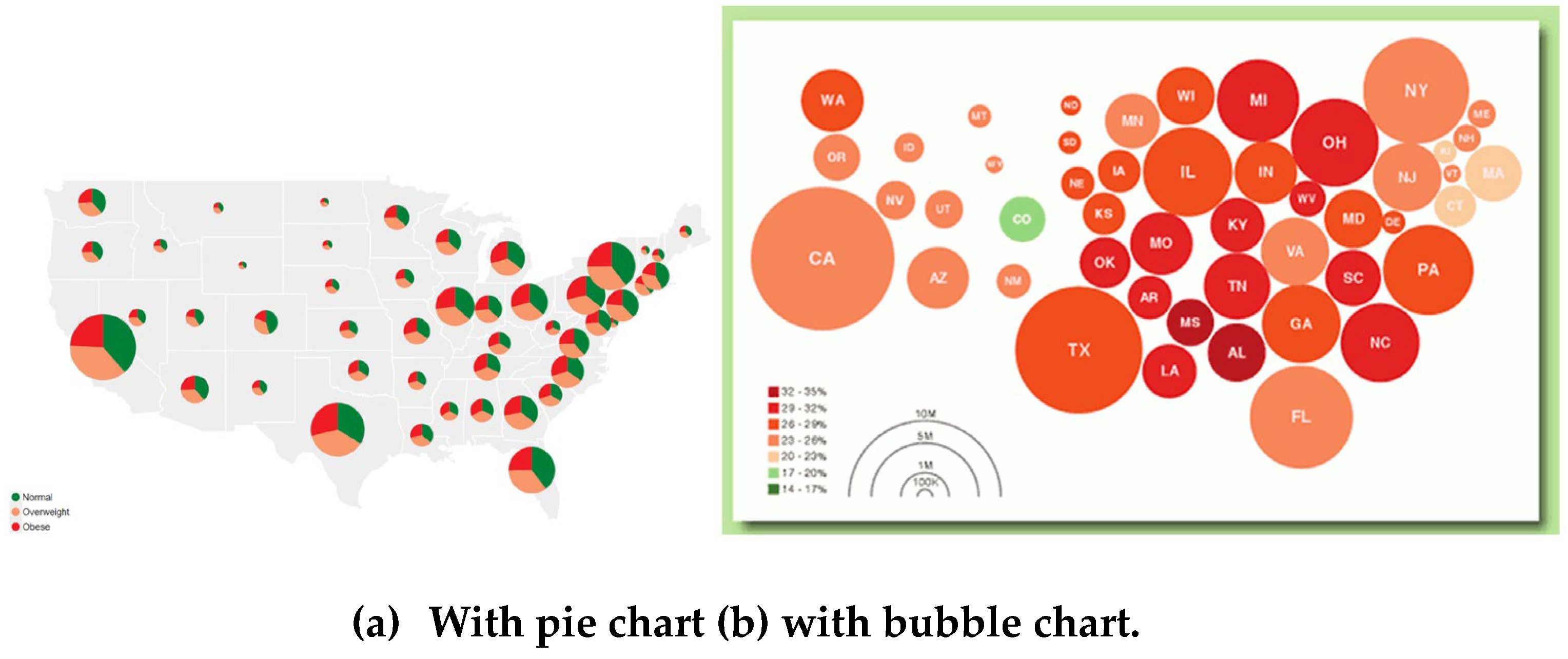
Figure 2.
The bubble chart for file system.
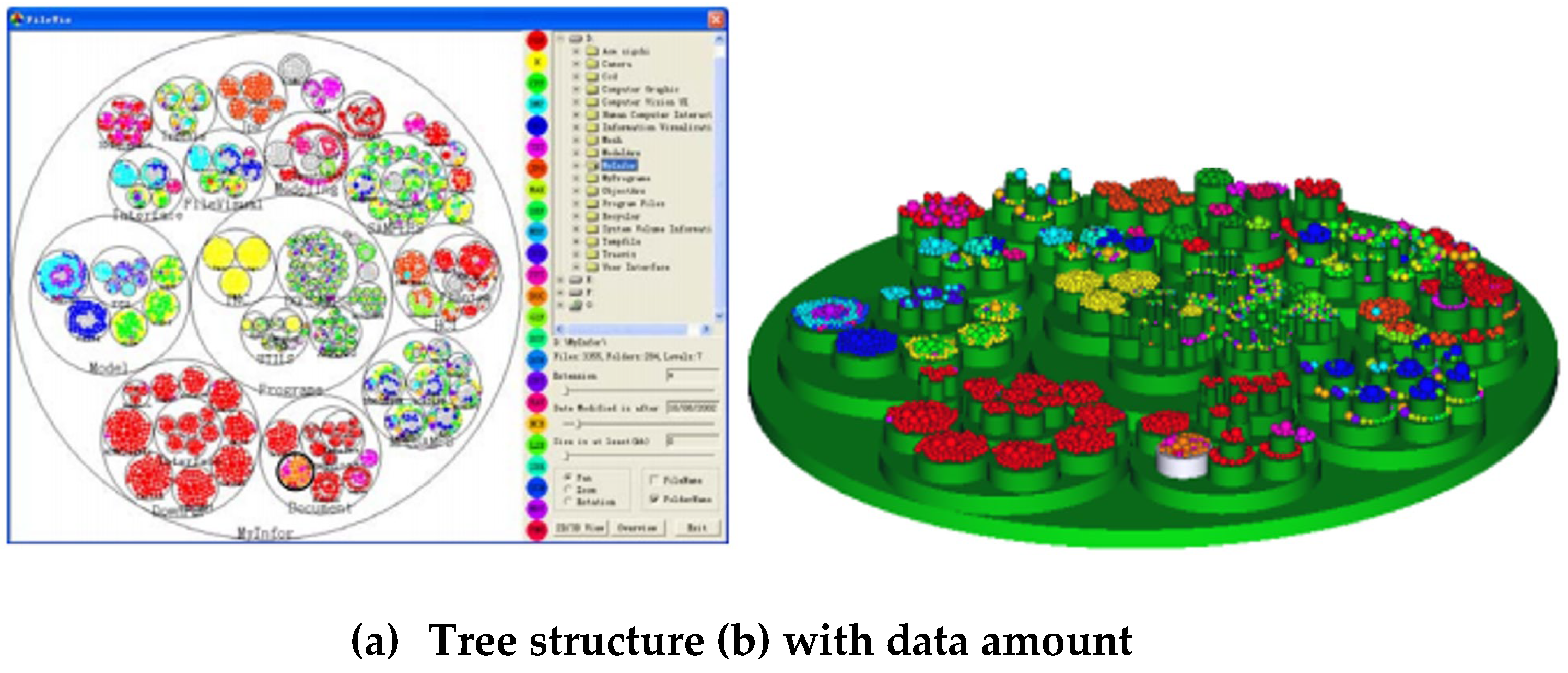
Figure 3.
Examples for BC[1,n], BC[1,n,n],BC[1,n,mn].
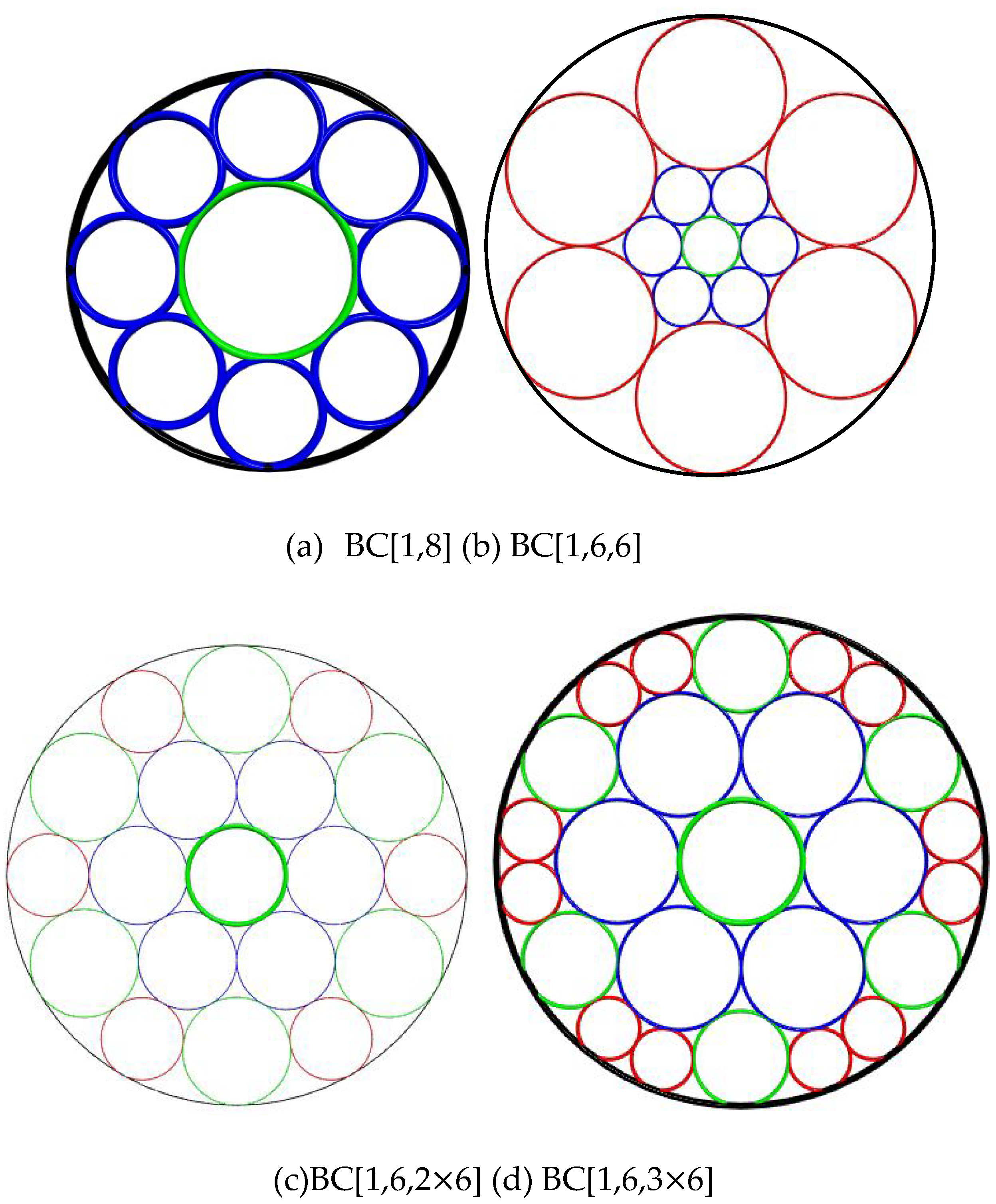
Figure 4.
Circle chain and Circle ring.
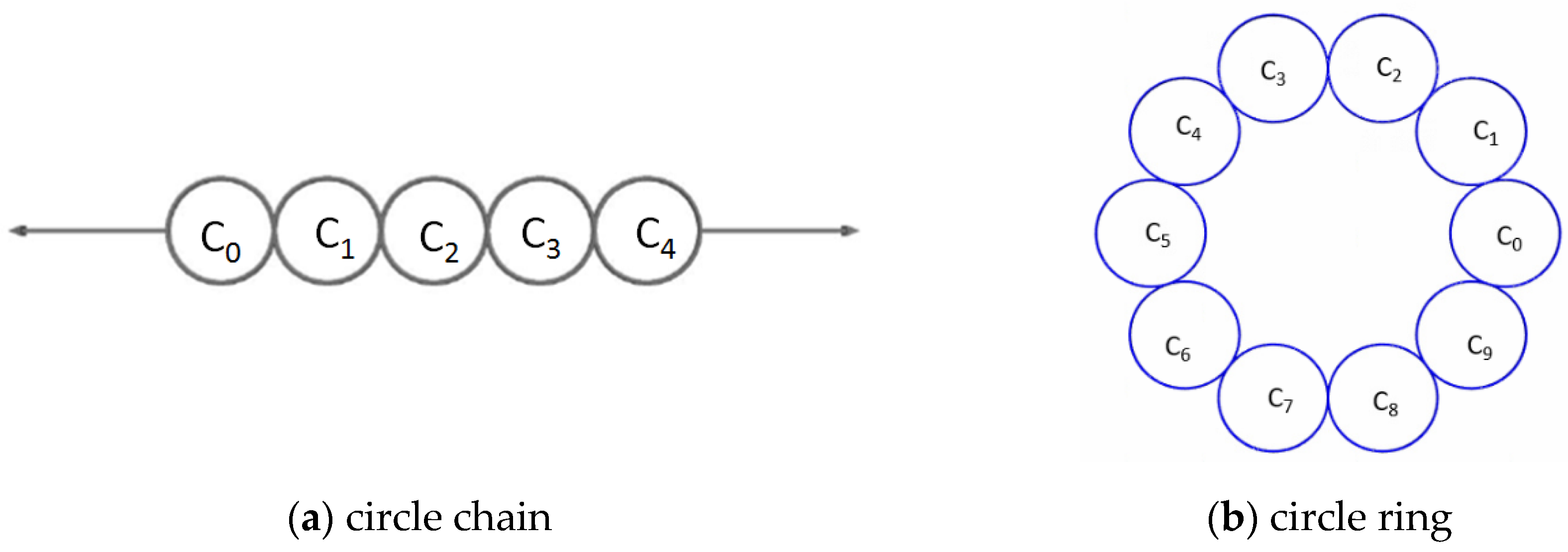
Figure 5.
Bubble chart for BC[1,n] problem.
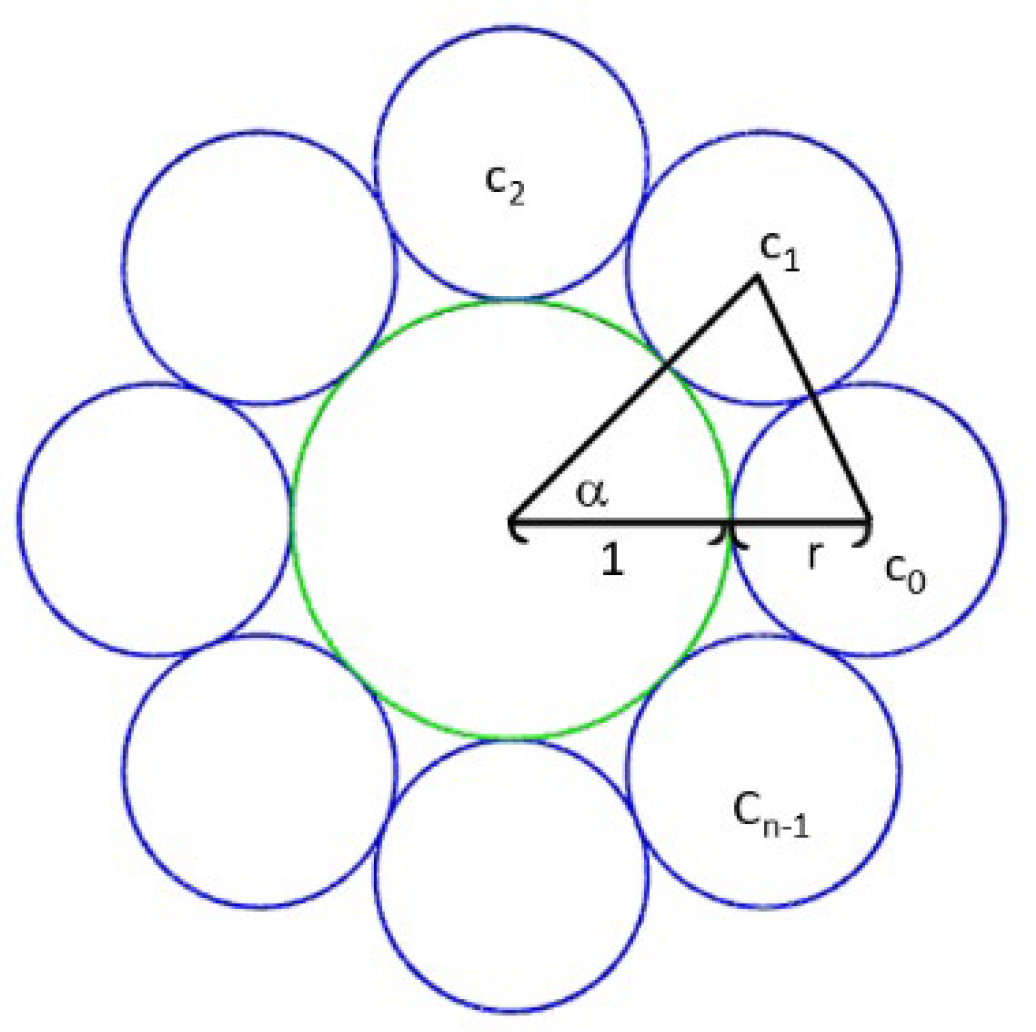
Figure 6.
The second layer of bubble chart.
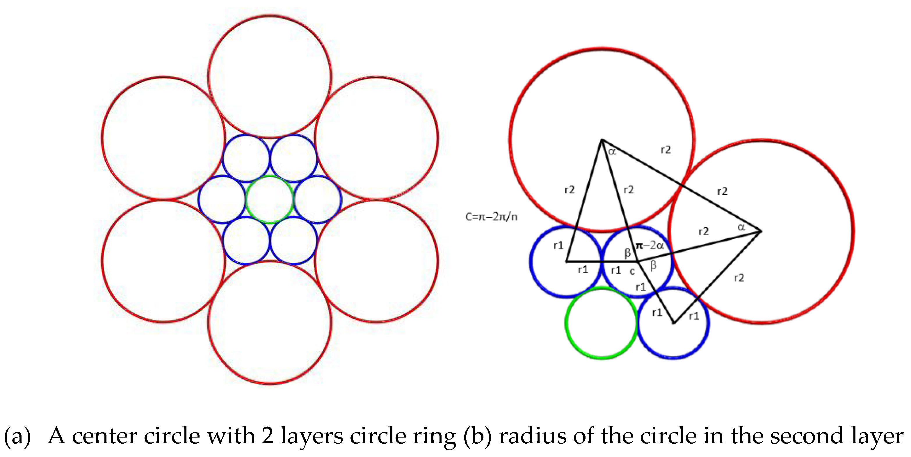
Figure 7.
The radius for the silhouette circle.
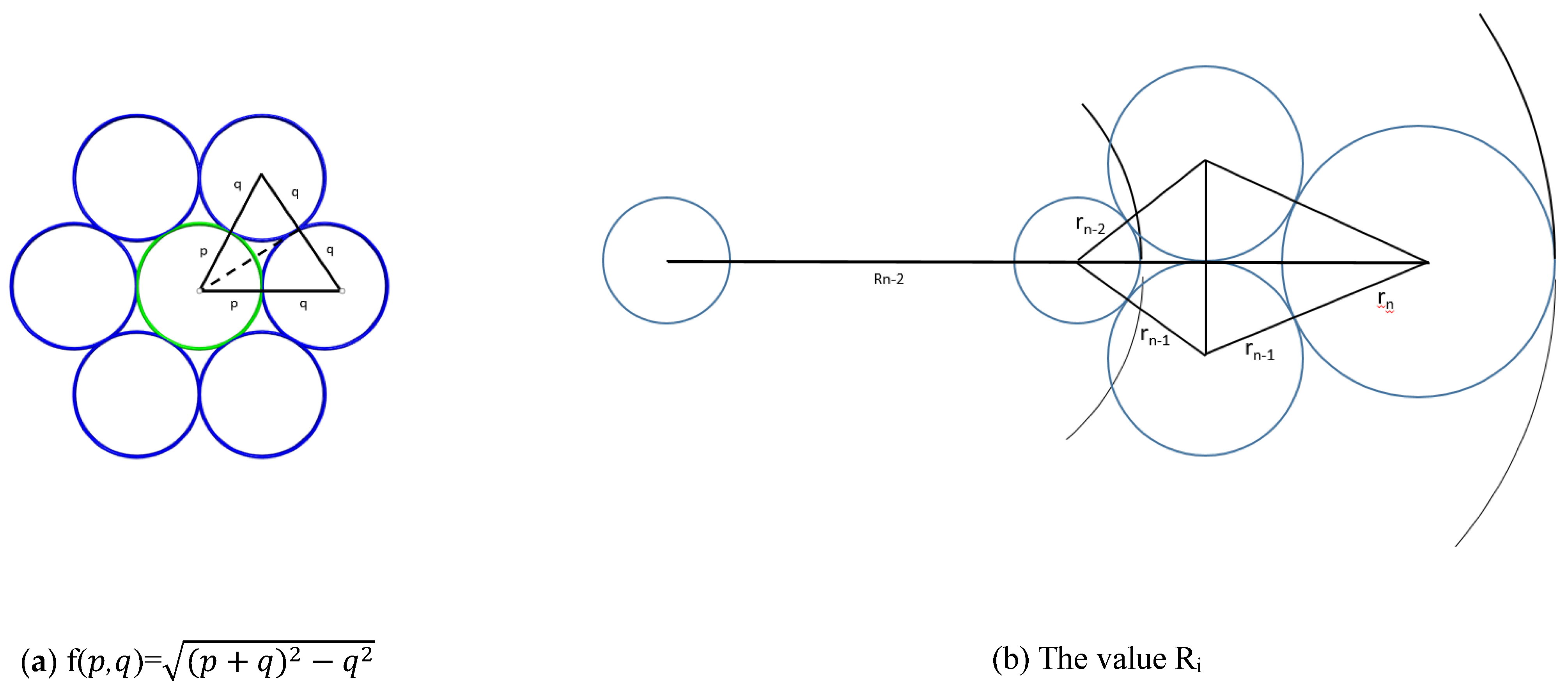
Figure 8.
Two different radii for the second layer.
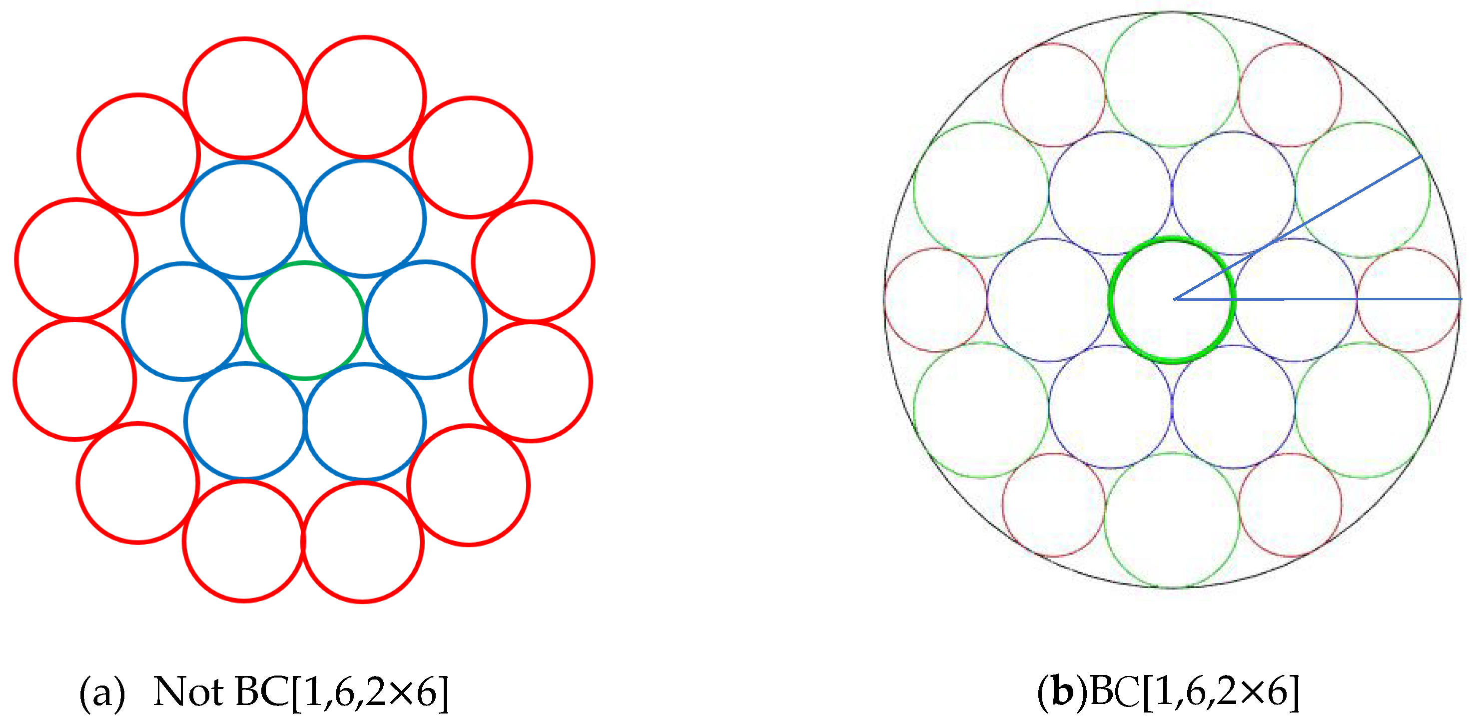
Figure 9.
Generate system of equation for BC[1,n,2n] problem.
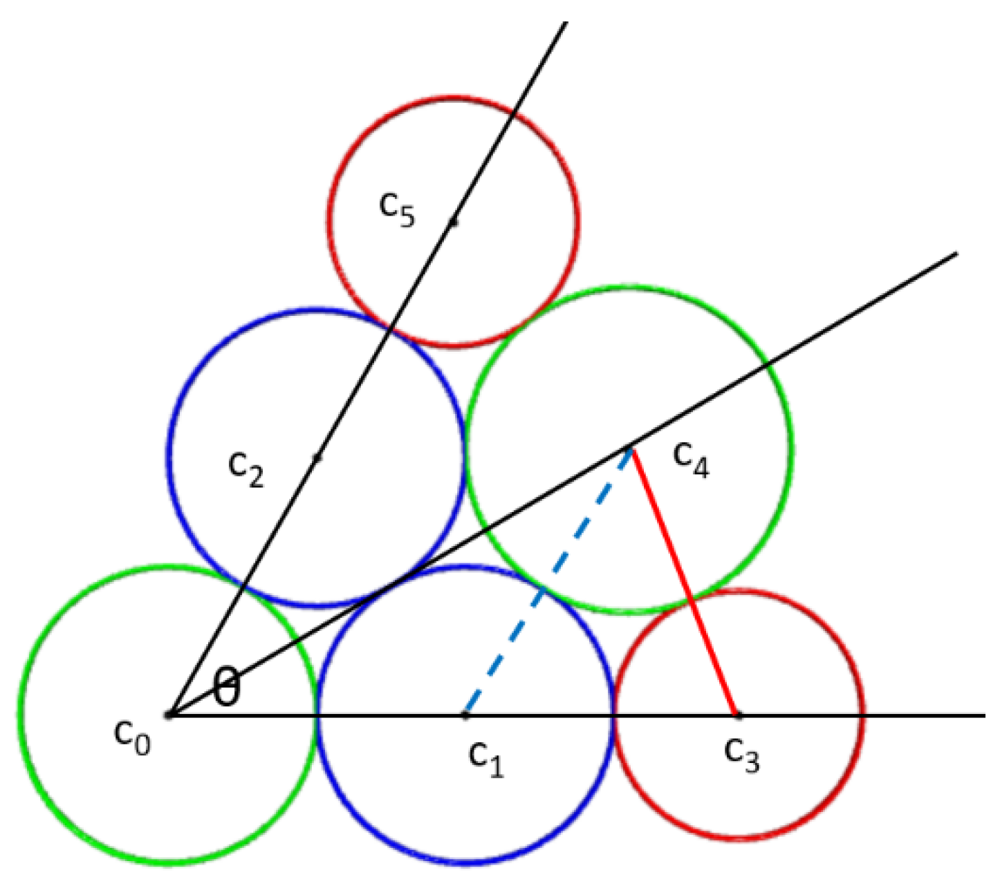
Figure 10.
The angle for three tangency circles.

Figure 11.
The sum of angles for a circle surround by circle ring.
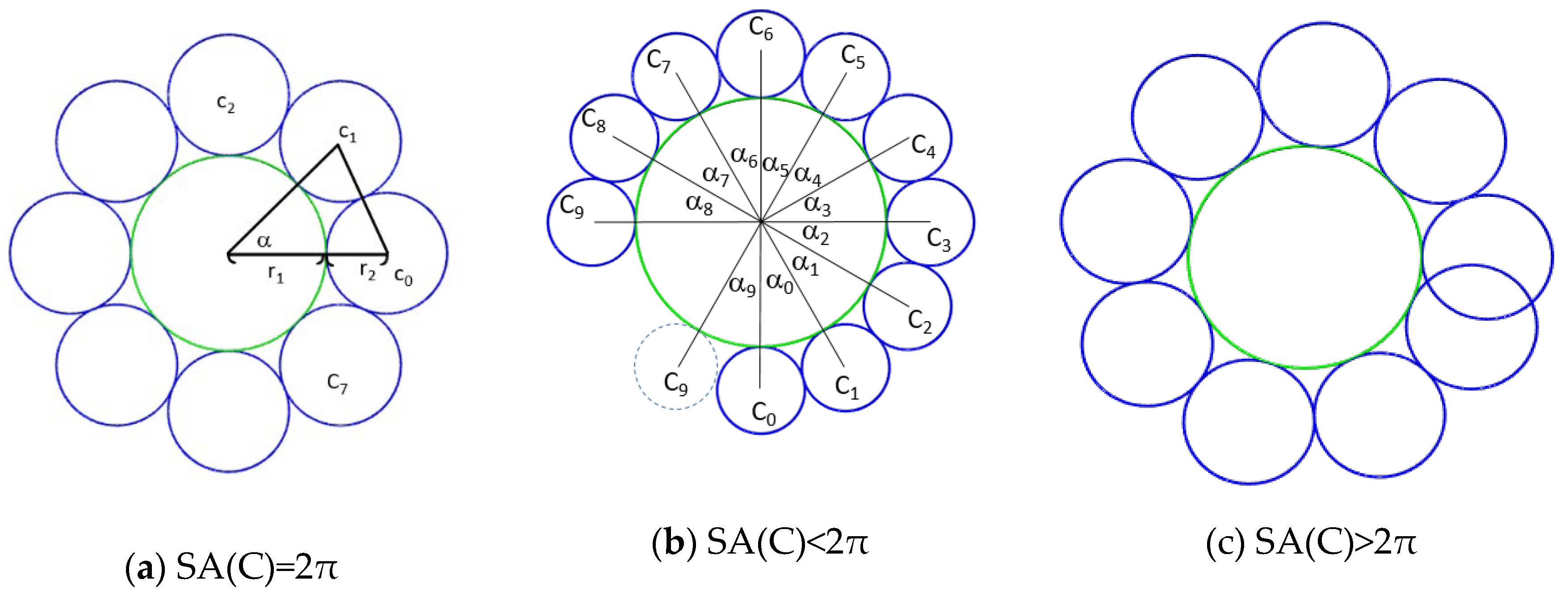
Figure 12.
Construct circle chain for second layer.
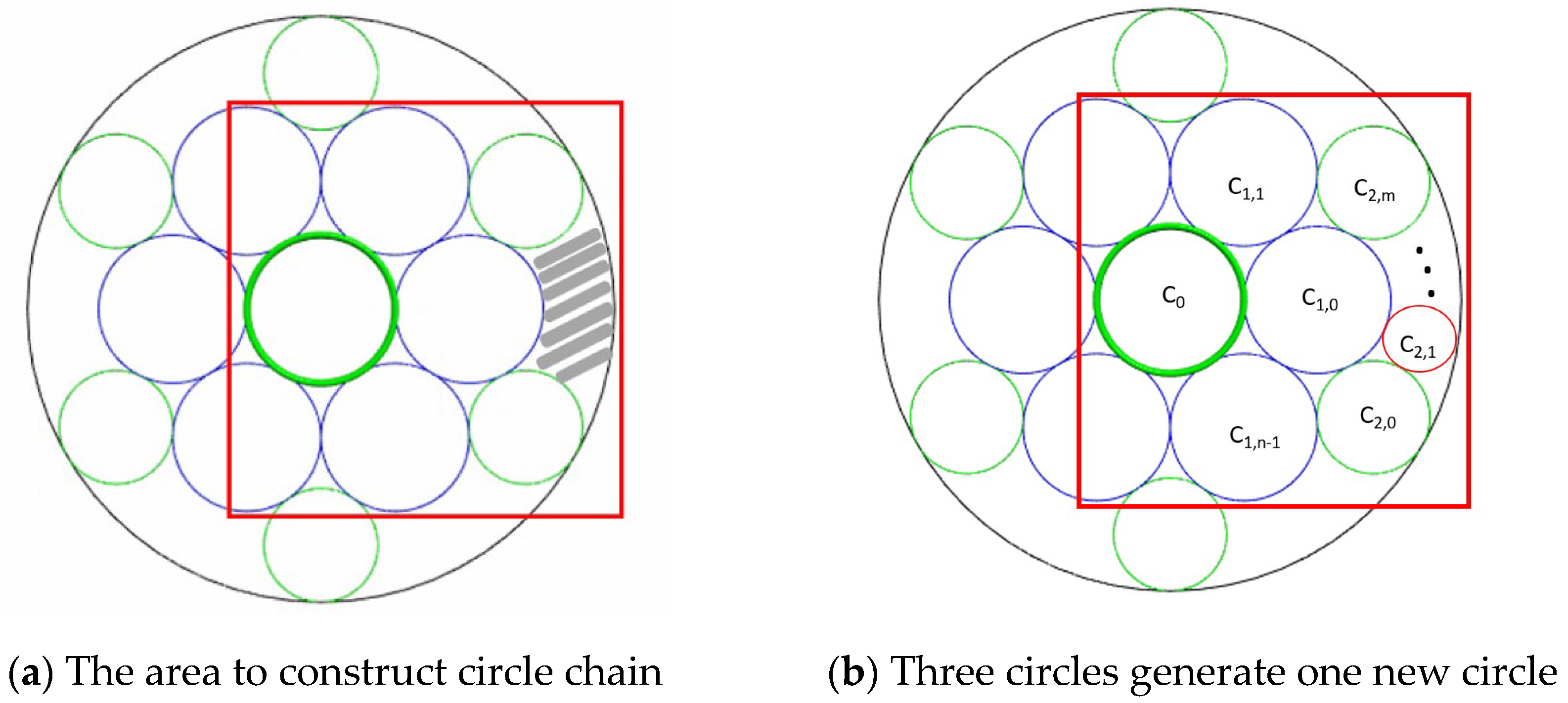
Figure 13.
Find two oriented circles tangent to three Oriented circles.
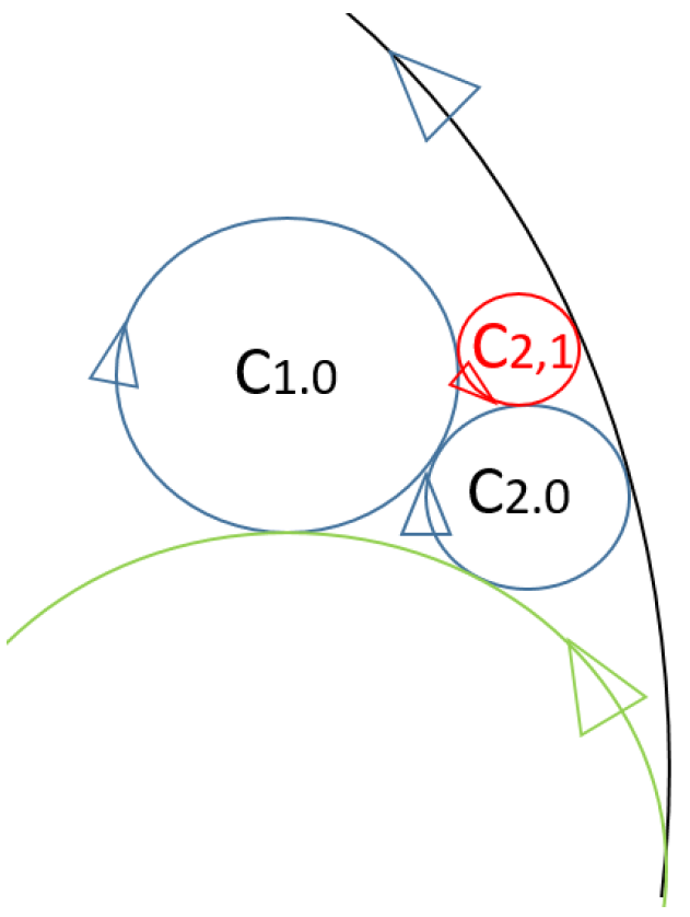
Figure 14.
BC [1, 7, mx7].
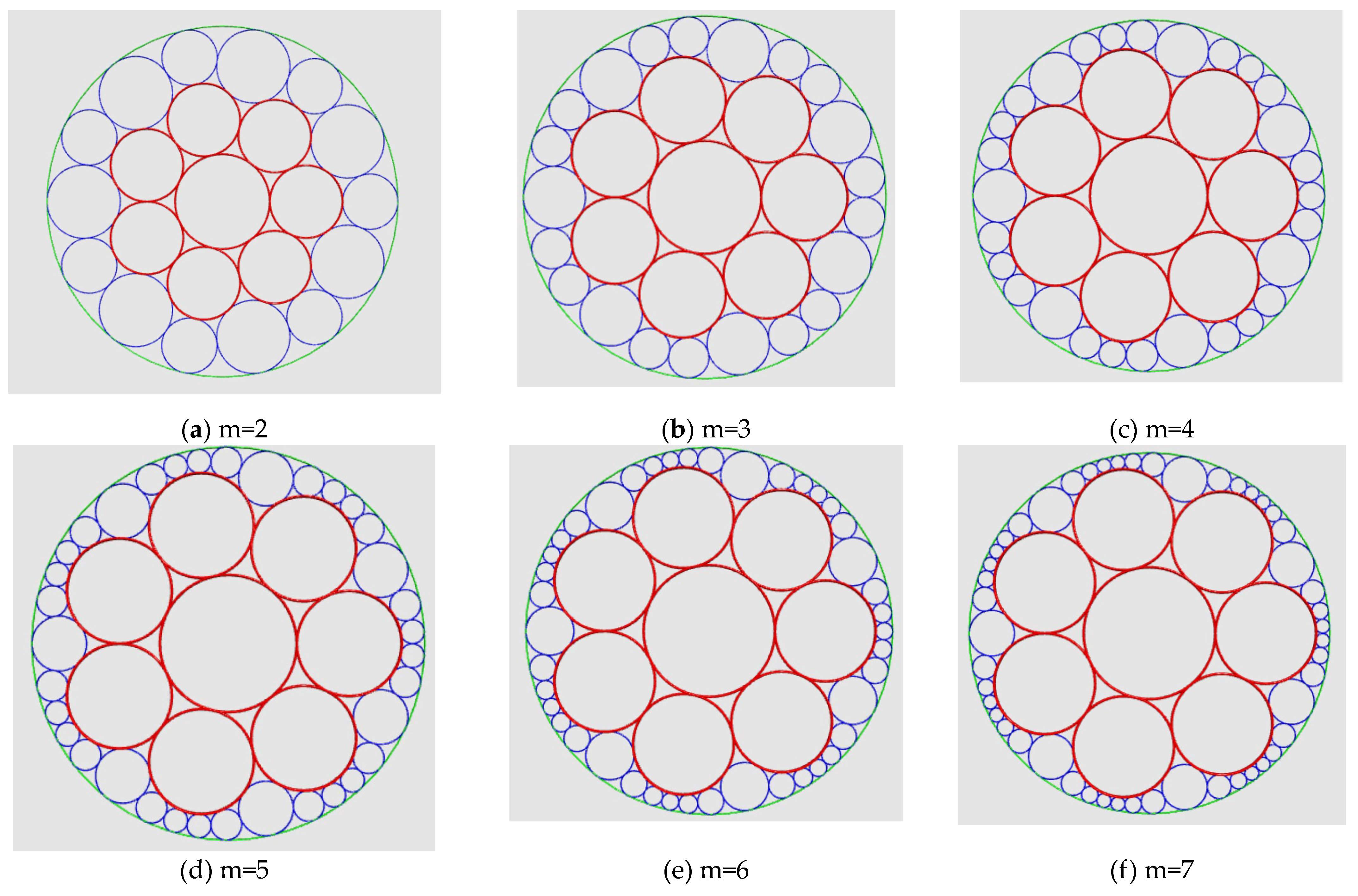

Table 1.
Radii for circles in BC[1,n,n,n,n,n,n] when n=5,6,7,8,9.
| n=5 | n=6 | n=7 | n=8 | n=9 | |
| (r1,R1) | (1.4259,3.851) | (1, 3.0) | (0.76642,2.5328) | (0.6199,2.239) | (0.5198,2.0396) |
| (r2,R2) | (4.5872,12.391) | (2.589,7.769) | (1.71413,5.6648) | (1.2463,4.503) | (0.96366,3.7812) |
| (r3,R3) | (14.757,39.863) | (6.70,20.123) | (3.8337,12.669) | (2.505,9.054) | (1.7865,7.01) |
| (r4,R4) | (47.473,128.241) | (17.372,52.119) | (8.5743,28.3361) | (5.0382,18.203) | (3.3120,12.995) |
| (r5,R5) | (152.724,412.554) | (44.995,134.978) | (19.176,63.374) | (10.129,36.599) | (6.1402,24.043) |
| (r6,R6) | (491.317,1327.19) | (116.538,349.613) | (42.889,141.744) | (20.366,73.585) | (11.383,44.666) |
Table 2.
The radii for the circles generated by Example.
| R | r20 | r21 | r22 | r23 | r24 | r25 | |
| 2 | 3.70021 | 0.7733 | 0.58368 | ||||
| 3 | 3.2118 | 0.55 | 0.35746 | 0.55 | |||
| 4 | 2.99341 | 0.4532 | 0.27012 | 0.23029 | 0.27012 | ||
| 5 | 2.87077 | 0.4 | 0.22555 | 0.17429 | 0.22555 | 0.4 | |
| 6 | 2.79374 | 0.3671 | 0.19934 | 0.14435 | 0.14435 | 0.19934 | 0.3671 |
| 7 | 2.74115 | 0.3449 | 0.18227 | 0.12608 | 0.10634 | 0.12608 | 0.18227 |
Disclaimer/Publisher’s Note: The statements, opinions and data contained in all publications are solely those of the individual author(s) and contributor(s) and not of MDPI and/or the editor(s). MDPI and/or the editor(s) disclaim responsibility for any injury to people or property resulting from any ideas, methods, instructions or products referred to in the content. |
© 2024 by the authors. Licensee MDPI, Basel, Switzerland. This article is an open access article distributed under the terms and conditions of the Creative Commons Attribution (CC BY) license (http://creativecommons.org/licenses/by/4.0/).
Copyright: This open access article is published under a Creative Commons CC BY 4.0 license, which permit the free download, distribution, and reuse, provided that the author and preprint are cited in any reuse.


