
Submitted:
18 December 2024
Posted:
18 December 2024
You are already at the latest version
Abstract
In urban engineering construction, ensuring the stability and safety of subsurface geological structures is as crucial as surface planning and aesthetics. This study proposes a novel multivariate radial basis function (MRBF) interpolant for three-dimensional (3D) modeling of engineering geo-logical properties, constrained by the stratigraphic structural model. A key innovation is the in-corporation of a well-sampled geological stratigraphical potential field (SPF) as an ancillary variable, which enhances the interpolation of geological properties in areas with sparse and uneven sampling points. The proposed MRBF method outperforms traditional interpolation techniques by showing reduced dependency on the distribution of sampling points. Furthermore, the study calculates the bearing capacity of individual pile foundations based on precise stratigraphic thicknesses, yielding more accurate results compared to conventional methods that average these values across the entire site. Additionally, the integration of 3D geological models with urban planning facilitates the de-velopment of comprehensive urban digital twins, optimizing resource management, improving decision-making processes, and contributing to the realization of smart cities through more efficient data-driven urban management strategies.
Keywords:
interpolant
; multivariate radial basis function
; three-dimensional geological modeling
; engineering geological property model
; bearing capacity of pile foundation
1. Introduction
In urban engineering construction, the development of a fine-grained engineering geological model is critical not only for enhancing engineering geological work and digital city framework but also for the quantitative evaluation of the urban environment, urban planning, subsurface space development, and rapid disaster response [1,2]. The three-dimensional (3D) visualization and characterization of geologic bodies offer a more realistic and intuitive depiction of subsurface geologic structures and properties [3]. Since Houlding (1994) introduced the concept of 3D geological modeling [4], it has been a vital tool in geological information processing and scientific research. Three-dimensional geological modeling comprises two key components, i.e., structural modeling and property modeling. Structural modeling involves constructing models by combining geometric entities, i.e., points, lines, surfaces, and bodies, with a focus on the shape of geological structures and their interrelationships. Property modeling, on the other hand, divides the 3D geological space into regular or irregular voxels, focusing on the spatial distribution of physical and chemical properties. Property models can be seamlessly integrated with geophysical fields [5,6,7], geochemical fields [8,9,10], structural analysis [11,12,13], metallogenic analysis [14,15], and reservoir characterization [16,17,18].
Spatial interpolation is a fundamental technique for property modeling, wherein the properties of sampling points are used to infer the properties of points to be estimated. Commonly used interpolation methods include Kriging [19,20,21], discrete smooth interpolation (DSI) [22,23], inverse distance weighted (IDW) [24,25], and radial basis function (RBF) [26,27,28]. The performance of spatial interpolation is significantly influenced by data density and the spatial distribution of sample points [29]. Generally, well-sampled ancillary variables that provide useful information about the under-sampled primary variable should be considered. Wang et al. (2005) compared cokriging (CK) and ordinary Kriging (OK) methods to estimate the quantity and distribution of soil chemicals from a limited number of available samples, showing that cokriging of half of the observations, using the same number of samples for the secondary variable (total salt), resulted in more accurate results than OK of all the samples [30]. Guastaldi et al. (2013) demonstrated that multivariate cokriging spatial interpolation of the under-sampled primary airborne gamma-ray data, using a well-sampled geologic map as ancillary variable, exhibited a distinct correlation between geological formations and radioactivity contents [31]. Zhu et al. (2013) transformed qualitative geological constraints into quantitative control parameters during data preprocessing and applied different property interpolation schemes to different types of geo-objects, resulting in geologically reasonable property models controlled by geological structures [32]. Foehn et al. (2018) explored the regression cokriging approach to efficiently combine weather radar data with data from two heated rain gauge networks of different quality, demonstrating the added value of the radar information compared to using only ground station data [33]. Liu et al. (2024) developed a multivariate spatial interpolation method based on Yang-Chizhong filtering (CoYangCZ), integrating geometry and statistics-based strategies to improve accuracy of a variable of air pollution using ancillary meteorological datasets [34]. However, the accuracy of these methods largely depends on the sufficient number and proper distribution of sampling points. In practice, the number of geological property sampling points is often limited and unevenly distributed due to high costs. Additionally, geological property interpolation that only considers the spatial distance and direction effects between scattered points is insufficient. In 3D geological space, a stratum deposited during the same geological era will exhibit strong similarity in its physical and chemical properties, e.g., lithology and materials, even when spatial distances are maximum.
Geological property is strata-bound, and its interpolation should be conducted under the constraints of the geological structures [32]. A 3D stratigraphic potential field (SPF), using an implicit mathematical function, describes the continuous stratigraphic distribution and represents geological boundaries [35]. Using SPF to express a set of conformable strata in 3D space is convenient for spatial analysis, statistics, and simulation. This study proposes the multivariate RBF (MRBF), incorporating the SPF as an ancillary variable into the engineering geological property interpolation algorithm to achieve strata-bound results. The property model is constructed using a hexahedral grid, with the properties of each grid cell interpolated using the MRBF algorithm. Three properties, i.e., natural water content, natural pore ratio, and water saturation, are modeled with the constraints of the 3D SPF model. The proposed method provides a more precise tool for modeling subsurface geological conditions, which is crucial for designing safe and stable foundations in urban engineering construction. Subsequently, the bearing capacity of the pile foundation for each building is designed and calculated. By accurately calculating pile foundation bearing capacity based on detailed stratigraphic models, this study minimizes geotechnical risks and enhances construction safety. Finally, the surface building inclined photogrammetric models are integrated with the subsurface 3D engineering geological models.
2. Method
2.1. Multivariate Radial Basis Function (MRBF)
2.1.1. RBF Interpolation
RBF interpolation involves constructing a linear combination of RBFs from sampling points, where the RBF value typically depends on the distance between the point to be interpolated and the sampling points [36]. Given discrete property points , where denotes the position of the point i, and fi denotes the property value at the point i, the interpolation function can be expressed as follows:
where N is the total number of RBFs used for interpolation, represents the generalized form of the RBFs used, denotes the Euclidean distance between the position vectors of and , and is the corresponding weight coefficient. The commonly used RBFs are listed in Table S1.
By substituting the coordinates and the corresponding property values , the equations can be expressed in matrix form as follows:
where. The weight coefficients can be calculated by solving the linear system of equations. Once the coefficients are determined, the interpolation function can be obtained, and the property values can be calculated by substituting the coordinates of the points to be interpolated.
2.1.2 MRBF Interpolation
When an attribute filed exhibits linear characteristics, these linear characteristics can also be incorporated into the RBF interpolant [37,38]. Inspired by this, when interpolating the properties of the strata, especially when the number of sampling points is limited, we can introduce an SPF model, which reflects the depositional order of the strata, as an auxiliary variable to enhance the property interpolation. This approach helps control the overall strata-bound trend of the properties, thereby improving the validity of the interpolation results.
The stratigraphic interface is represented by a specific equipotential surface of the SPF . The SPF values with a stratum change gradually from bottom to top, reflecting the temporal order of stratum deposition [35,39]. When the number of sampling points for property values is limited, an interpolation function can be established, assisted by the known SPF values as ancillary variables. The SPF can be estimated using an RBF interpolant, allowing the final interpolation function to be expressed as follows:
where is the RBF, and is the estimated SPF function. There are parameters to be solved, i.e., (i=1, 2, ..., n) are the weighting coefficients of the RBF,
is the weighting coefficient of the SPF, and β is a constant term to reduce interpolation error when the point to be interpolated is far from the sample points. With n coordinates and corresponding property values from sampling points, to obtain n+2 weighting coefficients requires the orthogonality conditions of the basis functions, as follows:
Thus, there are equations, which can be expressed in matrix form. The solution for the parameters can be determined, allowing the interpolation function to be specified as follows.
where .
2.2. Verification Experiments
2.2.1. Experiment Models
To verify the effectiveness of the proposed MRBF interpolation method, a two-dimensional (2D) experimental model was generated to compare this method with existing common interpolation methods. The property field of the experimental model is defined by the equation , where the region scope is . The property values range from -2.08 to 6, with an average value of approximately 2.9245. Based on the distribution of the property field, a distance function was selected as the ancillary model for multivariate interpolation. The experimental model and the ancillary model are illustrated in Figure 1. The correlation coefficient r between f and P is -0.9804, indicating a significant negative correlation, validating their use for co-interpolation.
A set of sample points with known property values fi were randomly generated, as shown in Figure 2a. Additionally, 31×21 sampling points for the ancillary variable Pj were obtained using uniform sampling with a 5m interval, as shown in Figure 2b. Their coordinates and ancillary variable values are then substituted into the RBF interpolation formula to calculate P(u). Grid points served as the points to be interpolated, which were compared to the true values.
Thirty experiments, each with 20 randomly generated sampling points and corresponding property values, were conducted. The MRBF interpolation results using four radial basis functions, i.e., cubic, linear, Gaussian, and thin plate, were compared, as shown in Figure S1. The results clearly demonstrate that the cubic function consistently outperforms the other three RBFs, both in terms of maximum and average errors.
2.2.2. Interpolation Results
By comparing the original model, it indicates that there is no significant difference between the interpolation results and the true values, as shown in Figure 3a. To further evaluate the accuracy, Figure 3b presents a scatter plot with the true values as the horizontal axis and the interpolation results as the vertical axis. The line signifies perfect consistency between true and interpolated values. Most points are distributed near the line , indicating a high degree of consistency. The interpolation results tend to be slightly smaller than the true values at lower values and slightly larger at higher values. Figure 3c illustrates the distribution of absolute errors. The maximum absolute error is 0.39, with an average error of 0.041, demonstrating a high degree of interpolation accuracy. Data points with large absolute errors are primarily located in the lower left corner, corresponding to areas with sparse sampling points.
2.2.3. Influence of Number of Sampling Points
In addition to the proposed MRBF interpolation algorithm, several other commonly used interpolation algorithms, i.e., IDW, ordinary Kriging (OK), and DSI, were employed to assess the effectiveness of the MRBF algorithm. To demonstrate the superiority of our proposed method, we randomly sampled 10, 20, and 30 points, as shown in Figure S2, and conducted the interpolation method comparison, as shown in Figure S3.
We evaluated these methods using three evaluation metrics of maximum absolute bias (MABS), mean absolute error (MAE), and mean square error (MSE).
MABS measures the largest absolute difference between interpolated and true values, indicating the worst-case error.
MAE computes the average absolute differences between interpolated and true values, reflecting overall accuracy.
MSE calculates the average of the squared differences between interpolated and true values, emphasizing larger errors.
Table S2 reveals that the MRBF method proposed in this study consistently outperforms other methods across different numbers of sampling points. Even with a decrease in sampling points, the MRBF method still maintains robust interpolation performance. Overall, the interpolation methods are sorted by performance as follows: MRBF > Kriging > DSI > IDW. Notably, MRBF demonstrates superior interpolation performances even with a limited number of sampling points. The Kriging interpolation exhibits instability when sampling points are limited or when the variogram fitting is inaccurate, reducing its overall performance. While RBF ranks second after MRBF with 30 and 20 sampling points, it shows poorer performance with only 10 sampling points, with an MAE of 6.529. This discrepancy may stem from RBF’s stringent requirement for uniformly distributed sampling points.
2.2.4. Influence of Distribution of Sampling Points
To investigate whether MRBF faces similar challenges related to the spatial distribution of sampling points, we conducted experiments with 18 sampling points using both random and uniform sampling methods. Figure S4 illustrates the spatial distribution of these sampling points, and Figure S5 presents the interpolation results for each algorithm under both scenarios.
As shown in Table S3, when the sampling points are uniformly distributed, the accuracy of RBF interpolation significantly improves compared to random distribution. This underscores RBF’s requirement for uniformly distributed sampling points. In contrast, the MRBF interpolation shows only marginal improvement, indicating that the ancillary variable integration in MRBF relaxes the uniformity requirement for sampling points and maintains robust interpolation results even with sparse distributions. Among all the methods, Kriging’s performance suffers from poor variogram fitting over uniformly distributed sampling points, leading to unreliable results. Under random sampling, although Kriging exhibits the smallest MABS value, its MAE and RMSE value are larger than those of MRBF, placing it second after MRBF. IDW and DSI methods exhibit similar performance, showing less sensitivity to sampling point uniformity.
In summary, the proposed MRBF interpolation algorithm incorporates an ancillary variable to control the overall trends. The results of the verification experiments, conducted using a 2D model, demonstrate superior accuracy compared to the other commonly used interpolation methods. MRBF maintains robust performance with fewer sampling points, and mitigates RBF’s uniformity requirement drawback, enabling itself as an effective and stable interpolation technique. Moreover, this algorithm allows for the inclusion of any other relevant variable. When the number of sampling points of the main variable is insufficient, another variable with more sampling points related to it can be selected as an ancillary variable to assist interpolation, which can improve the interpolation accuracy to a certain extent and make the interpolation of variables with limited sampling points possible.
3. Case Study
3.1. Dataset
The data source for this case study is the detailed geotechnical investigation dataset of a building site at the stage of construction drawings design. As shown in Figure 4, the construction site is located beside South Zhengyang Road in Hengyang City. Its geomorphology is characterized by the Xiangjiang III terrace landform, relatively flat and open, with ground elevations ranging from 84.45m to 87.17m. The site is situated in the South China Fracture Zone, within the Hengyang Basin, which lies in the middle and lower part of the Yangtze River Faulted Depression. This area is a Cretaceous-Tertiary terrestrial stabilized basin. The site’s stratigraphy belongs to the Tertiary inland lake sedimentary, predominantly composed of clastic rocks. The regional tectonics are dominated by the Xishan Stage, with two main groups of NNE and NNW oriented. There are no traces of large faults passing through the site or its neighboring lots, and recent tectonic activity, especially newly active rupture structures, is not evident, indicating the site is in a relatively stable status. According to geological drilling results, the exposed strata within the exploration depth of this construction site include plain fill soil (Q4ml), silty clay (Q4al), gravelly sand (Q4al), clay (Q4el), and the Lower Tertiary (E) mudstone.
The dataset used for modeling include 37 borehole histograms, 16 engineering geological cross-sections (Figure 5a), a location map of buildings and exploration points (Figure 5b), and an experimental report of physical and mechanical properties containing 41 soil samples. Five buildings are planned for construction, with exploration completed for buildings 1#, 2#, and 3#, as shown in Table S4. Figure 6 shows an example of an engineering geologic cross-section 2-2’.
The surface building model is an inclined photogrammetric dataset in OSGB (open scene graph binary) format. Figure 7 shows the surface buildings in the vicinity of the site. The total planned land area is 18,306.1 m², and the total building area is 95,211.6 m².
3.2. Geological Structural Modeling
Geological cross-sections combine of original engineering geological investigation data with expert interpretation, making them suitable for 3D modeling of stratigraphic contact surfaces. In this study, the 16 cross-sections interpreted by engineer geologists were processed to obtain a series of stratum boundaries. These boundaries were then stitched up according to the strata. Subsequently, the surface model with the stratigraphic undulation pattern was constructed based on the DSI algorithm. Finally, the boundaries were stitched together to generate a solid model. The 3D geological structure modelling process is shown in Figure 8. The volume and average thickness of each stratum were calculated, as shown in Table 1.
Groundwater at the site consists primarily of loose rock pore water, predominantly stored within the gravel sand layers. It is recharged by infiltration of atmospheric precipitation and lateral flows from surrounding aquifers, discharging towards lower-lying areas, particularly to the east and northeast border of the site, exhibiting dynamic variability and generally adequate water content. The groundwater levels (GWLs) in the boreholes range between 1.9 m and 20.0 m in depth, with elevations spanning from 66.91 m to 83.45 m. Figure 9 illustrates that the GWL surface aligns with the bottom surface of the gravel-sand layer, highlighting it as the principal aquifer and flow conduit on the site. Groundwater flow generally trends from southwest to northeast.
3.3. Geological Property Modeling
The solid model was grided into cells with size of 1m×1m×0.2m, where the cell properties were filled with the values at the cell center. Three properties, i.e., natural pore ratio, natural moisture content, and water saturation, were selected for modeling according to the experimental report of physical and mechanical properties of soil samples. The SPF values of the stratum surfaces were set to 10, 20, 30, 40, and 50 from top to bottom. The SPF values at points between the stratum surfaces were obtained using the IDW interpolation method (Figure 10). The SPF model was uniformly sampled under the structural constraints of the strata and used as a covariate to assist in the main variable interpolation. We employed the MRBF method to interpolate the properties of the entire model. Since the properties vary among different strata while being similar within the same stratum, this interpolation was conducted under the constraints of the stratum. Specifically, the interpolation was performed separately for the silty clay, clay, and mudstone layers. The interpolation results are visualized in Figure 11, and the histogram illustrates the distribution of the properties values of each stratum, as shown in Figure 12. The distribution of the moisture content and pore ratio revealing a similar pattern, suggesting a possible correlation between them.
4. Discussions
Based on the 3D geological models and the engineering geological conditions of the site, combined with the engineering scale of the proposed buildings, it is recommended to adopt prestressed pile foundation, using the strongly weathered mudstone layer as the bearing layer. The expected length of the piles is 20.0~25.0 m (measured from the basement floor), and the diameter of the piles is 400~500 mm. The pile bearing capacity is determined according to the analysis and statistical results of geotechnical in-situ and indoor tests. Drawing insights from Chinese standards [40,41], construction industrial standards [42], and regional past engineering experiences [43], the pile bearing capacity calculation formula is expressed as follows:
where is the standard value of total ultimate lateral resistance, is the standard value of total ultimate end resistance, μ is the perimeter of pile body, is the standard value of ultimate lateral resistance of the ith layer of soil on the side of the pile, is the thickness of the ith layer of soil on the side of the pile, is the correction coefficient of the pile end resistance (taking 0.9), is the standard value of the ultimate end resistance, and is the area of the pile end. The values of and generally derived from local experiences, as shown in Table S5.
The plain fill soil and silty clay layers will be completely excavated during construction, so their lateral resistance is not considered. Except for the strongly weathered mudstone layer, other layers cannot serve as the bearing stratum due to inadequate capacity. Therefore, only the strongly weathered mudstone layer is used to calculate the standard value of ultimate end resistance, taken as half of this standard value for estimation purpose. The actual characteristic value of the bearing capacity of a single pile should be determined through pile load tests and adjusted based on the test results if necessary.
The pile length is set to 25.0 m, measured from the basement floor at an elevation of 78m. As shown in Figure 13a, 491 piles were arranged in a full pile configuration, with a diameter of 500 mm and a spacing of 2000 mm between piles. The thickness of the pile foundation through each soil layer was calculated from the coordinates of the intersection points between the pile foundation and each horizon surface. The standard value of the bearing capacity of each pile is illustrated in Figure 13b. Tables S6–S8 present the characteristic values of bearing capacity for each pile. The characteristic value of the bearing capacity of the building is taken as the minimum value of the pile bearing capacity. Table 2 shows the characteristic values of the pile bearing capacity of each building, all of which exceed the maximum axial force of a single column, 2000 kiloNewton (kN). This indicates that the bearing capacity of the prestressed piles is adequate. Using conventional calculations based on the average thickness of each soil layer, we obtained a characteristic value of pile bearing capacity of 2333.11 kN, which is higher than the values calculated separately. The construction is designed according to the calculated value; if the actual bearing capacity is insufficient, it may lead to potential safety risks. For example, if the maximum shear stress is 2200 kN, the pile foundation bearing capacity calculated using the conventional calculation seems sufficient. In fact, some of the piles’ bearing capacity does not reached the 2200 kN, potentially causing safety risks and resource wastage. Our proposed method of calculating the bearing capacity of each pile foundation separately mitigates this issue, allowing for a clear identification of locations with weak bearing capacity.
The integrated surface building and subsurface engineering geological models are visualized in Figure 14. Integrating the processed surface buildings with the 3D geological models enables the expression of integrated spatial information in a digital city.
5. Conclusions
This study proposes a 3D geological property modeling method that incorporates SPF model to assist property interpolation with a limited number of sampling points. We achieved property interpolation based on the MRBF method under stratigraphic model constraints. Additionally, we calculated the characteristic values of pile foundation bearing capacity for each building, providing a more accurate reference for subsequent construction. Finally, we achieved an integrated representation of surface and subsurface space. The main conclusions are as follows:
(1) The proposed MRBF method effectively utilizes ancillary variable for multivariate interpolation, enabling relatively accurate interpolation with a few property sampling points. Experimental results from a 2D model indicate its high accuracy. The MRBF method outperforms several commonly used methods, i.e., IDW, DSI, and Kriging, particularly when the number of sampling points is limited. Additionally, the MRBF method’s performance remains stable regardless of the uniformity of sampling point distribution, making it robust for sparse sampling.
(2) A geological structural model was constructed based on cross-sections. We calculated the bearing capacity of each pile foundation individually rather than using an overall estimate based on average layer thickness, providing a more precise reference for construction. The GWL surface aligns closely with the bottom surface of the gravel sand layer, indicating that the site’s groundwater is primarily loose rock pore water stored in the gravel sand layer’s pore spaces.
(3) By interpolating property using the MRBF method under structural model constraints, we obtained property models consistent with stratigraphic deposition. Integrating the processed surface buildings with the 3D geological models enables the expression of integrated spatial information in a digital city.
Despite these advancements, this study has limitations concerning the MRBF method and the integrated model. The MRBF algorithm requires a significant correlation between primary and ancillary variables for meaningful multivariate interpolation. Without a strong correlation, adding an ancillary variable may introduce errors, reducing its performance. Future work should establish a standard for the required correlation strength. The integrated model could also offer more functionalities for managing, mining, analyzing, visualizing, and sharing geological models.
Supplementary Materials
The following supporting information can be downloaded at the website of this paper posted on Preprints.org, Figure S1 shows basis function comparison of MRBF interpolation performance of maximum absolute error and average error using different RBFs. Figure S2 presents sampling points’ numbers of 10, 20 and 30. Figure S3 depicts interpolation results of different methods with different numbers of sampling points. Figure S4 shows random vs. uniform spatial distributions of 18 sampling points. Figure S5 presents interpolation results for each method with randomly and uniformly spatial distributed sampling points. Table S1 shows commonly used RBFs. Table S2 presents performance of different interpolation methods with different number of sampling points. Table S3 depicts performances of different interpolation methods with different spatially distributed sampling points. Table S4 shows buildings’ workloads. Table S5 presents standard values of ultimate lateral resistance and ultimate end resistance. Table S6, S7, and S8 depict characteristic values of pile bearing capacity of buildings 1#, 2#, and 3#, respectively.
Author Contributions
Baoyi Zhang: Conceptualization, Validation, Writing—review and editing, and Funding acquisition; Yanli Zhu: Software, Data curation, and Writing—original draft preparation; Tongyun Zhang: Investigation and Data curation; Xian Zhou: Software; Binhai Wang: Writing—original draft preparation; Or Aimon Brou Koffi Kablan: Validation; Jixian Huang: Methodology, Software, and Writing—original draft preparation.
Funding
This study was supported by grants from the Scientific Research Project of Geological Bureau of Hunan Province (Grant No. HNGSTP202301), the Hunan Provincial Natural Resource Science and Technology Planning Program (Grant Nos. 20230123XX and HBZ20240144), and the National Natural Science Foundation of China (Grant No. 42072326).
Data Availability Statement
The dataset of the current study is not publicly available due to a data privacy agreement we signed with the Geological and Geographic Information Institute of Hunan Province, but are available from the corresponding author on reasonable request.
Acknowledgments
We thank SHI Yu-Zheng (Geological and Geographic Information Institute of Hunan Province) and ZOU Bin (Central South University) for their kind assistance in the data collection. Special thanks are extended to the MapGIS Laboratory Co-Constructed by the National Engineering Research Center for Geographic Information System of China and Central South University for providing the MapGIS® software (Wuhan Zondy Cyber-Tech Co. Ltd., Wuhan, China).
Conflicts of Interest
The authors declare no conflicts of interest.
References
- de Rienzo, F.; Oreste, P.; Pelizza, S. Subsurface geological-geotechnical modelling to sustain underground civil planning. Engineering Geology 2008, 96, 187–204. [Google Scholar] [CrossRef]
- Dou, F.; Li, X.; Xing, H.; Yuan, F.; Ge, W. 3D geological suitability evaluation for urban underground space development – A case study of Qianjiang Newtown in Hangzhou, Eastern China. Tunnelling and Underground Space Technol. 2021, 115, 104052. [Google Scholar] [CrossRef]
- Caumon, G.; Collon-Drouaillet, P.; Le Carlier de Veslud, C.; Viseur, S.; Sausse, J. Surface-Based 3D Modeling of Geological Structures. Mathematical Geosciences 2009, 41, 927–945. [Google Scholar] [CrossRef]
- Houlding, S. 3D Geoscience Modeling: Computer Techniques for Geological Characterization; Springer: Berlin, 1994. [Google Scholar]
- Lindsay, M.D.; Aillères, L.; Jessell, M.W.; de Kemp, E.A.; Betts, P.G. Locating and quantifying geological uncertainty in three-dimensional models: Analysis of the Gippsland Basin, southeastern Australia. Tectonophysics 2012, 546-547, 10–27. [Google Scholar] [CrossRef]
- de la Varga, M.; Schaaf, A.; Wellmann, F. GemPy 1.0: open-source stochastic geological modeling and inversion. Geoscientific Model Development 2019, 12, 1–32. [Google Scholar] [CrossRef]
- Zhang, B.; Xu, Z.; Wei, X.; Song, L.; Shah, S.Y.A.; Khan, U.; Du, L.; Li, X. Deep Subsurface Pseudo-Lithostratigraphic Modeling Based on Three-Dimensional Convolutional Neural Network (3D CNN) Using Inversed Geophysical Properties and Shallow Subsurface Geological Model. Lithosphere 2024, 2024. [Google Scholar] [CrossRef]
- Vollgger, S.A.; Cruden, A.R.; Ailleres, L.; Cowan, E.J. Regional dome evolution and its control on ore-grade distribution: Insights from 3D implicit modelling of the Navachab gold deposit, Namibia. Ore Geology Review 2015, 69, 268–284. [Google Scholar] [CrossRef]
- Zhang, B.; Chen, Y.; Huang, A.; Lu, H.; Cheng, Q. Geochemical field and its roles on the 3D prediction of concealed ore-bodies. Acta Petrologica Sinica 2018, 34, 352–362. [Google Scholar]
- Wang, L.F.; Wu, X.B.; Zhang, B.Y.; Li, X.F.; Huang, A.S.; Meng, F.; Dai, P.Y. Recognition of Significant Surface Soil Geochemical Anomalies Via Weighted 3D Shortest-Distance Field of Subsurface Orebodies: A Case Study in the Hongtoushan Copper Mine, NE China. Natural Resources Research 2019, 28, 587–607. [Google Scholar] [CrossRef]
- Hillier, M.; de Kemp, E.; Schetselaar, E. 3D form line construction by structural field interpolation (SFI) of geologic strike and dip observations. J. Struct. Geol. 2013, 51, 167–179. [Google Scholar] [CrossRef]
- Laurent, G.; Ailleres, L.; Grose, L.; Caumon, G.; Jessell, M.; Armit, R. Implicit modeling of folds and overprinting deformation. Earth and Planetary Science Letters 2016, 456, 26–38. [Google Scholar] [CrossRef]
- Grose, L.; Laurent, G.; Aillères, L.; Armit, R.; Jessell, M.; Cousin-Dechenaud, T. Inversion of structural geology data for fold geometry. Journal of Geophysical Research: Solid Earth 2018, 123, 6318–6333. [Google Scholar] [CrossRef]
- Zhang, B.; Xu, K.; Khan, U.; Li, X.; Du, L.; Xu, Z. A lightweight convolutional neural network with end-to-end learning for three-dimensional mineral prospectivity modeling: A case study of the Sanhetun Area, Heilongjiang Province, Northeastern China. Ore Geology Review 2023, 105788. [Google Scholar] [CrossRef]
- Basson, I.J.; Anthonissen, C.J.; McCall, M.J.; Stoch, B.; Britz, J.; Deacon, J.; Strydom, M.; Cloete, E.; Botha, J.; Bester, M.; et al. Ore-structure relationships at Sishen Mine, Northern Cape, Republic of South Africa, based on fully-constrained implicit 3D modelling. Ore Geology Review 2017, 86, 825–838. [Google Scholar] [CrossRef]
- Qiao, Z.F.; Shen, A.J.; Zheng, J.F.; Chang, S.Y.; Chen, Y.N. Three-dimensional carbonate reservoir geomodeling based on the digital outcrop model. Petroleum Explor. Dev. 2015, 42, 358–368. [Google Scholar] [CrossRef]
- Wang, L.X.; Yin, Y.S.; Zhang, C.M.; Feng, W.J.; Li, G.Y.; Chen, Q.Y.; Chen, M. A MPS-based novel method of reconstructing 3D reservoir models from 2D images using seismic constraints. J. Pet. Sci. Eng. 2022, 209, 10. [Google Scholar] [CrossRef]
- Mitten, A.J.; Mullins, J.; Pringle, J.K.; Howell, J.; Clarke, S.M. Depositional conditioning of three dimensional training images: Improving the reproduction and representation of architectural elements in sand-dominated fluvial reservoir models. Mar. Pet. Geol. 2020, 113, 20. [Google Scholar] [CrossRef]
- Matheron, G. Principles of geostatistics. Economic Geology 1963, 58, 1246–1266. [Google Scholar] [CrossRef]
- Marinoni, O. Improving geological models using a combined ordinary–indicator kriging approach. Engineering Geology 2003, 69, 37–45. [Google Scholar] [CrossRef]
- Sett, S.; Chattopadhyay, K.K.; Ghosh, A. Reliability-based seismic liquefaction hazard mapping of Kolkata Metropolitan City, India, using ordinary kriging technique. Bulletin of Engineering Geology and the Environment 2024, 83. [Google Scholar] [CrossRef]
- Mallet, J.L. Discrete smooth interpolation in geometric modelling. Comput.-Aided Des. 1992, 24, 178–191. [Google Scholar] [CrossRef]
- Caumon, G.; Sword, C.H.; Mallet, J.-L. Interactive Editing of Sealed Geological 3D Models. In Proceedings of the International Association for Mathematical Geology, Berlin, Germany, 2003.
- Lu, G.Y.; Wong, D.W. An adaptive inverse-distance weighting spatial interpolation technique. Computer & Geoscience 2008, 34, 1044–1055. [Google Scholar] [CrossRef]
- Li, Z. An enhanced dual IDW method for high-quality geospatial interpolation. Scientific Reports 2021, 11, 9903. [Google Scholar] [CrossRef] [PubMed]
- Powell, M.J.D. Radial basis functions for multivariable interpolation: a review. In Algorithms for approximation, PictureJ. C. Mason, P.G.C., Ed.; Clarendon Press: Imprint of Oxford University Press 198 Madison Avenue New York, NYUnited States, 1987; p. 694. [Google Scholar]
- Hillier, M.J.; Schetselaar, E.M.; de Kemp, E.A.; Perron, G. Three-Dimensional Modelling of Geological Surfaces Using Generalized Interpolation with Radial Basis Functions. Mathematical Geosciences 2014, 46, 931–953. [Google Scholar] [CrossRef]
- Qian, Y.L.; Shi, J.; Sun, H.Q.; Chen, Y.Y.; Wang, Q. Vector solid texture synthesis using unified RBF-based representation and optimization. Visual Computer 2023, 39, 3963–3977. [Google Scholar] [CrossRef]
- Li, J.; Heap, A.D. Spatial interpolation methods applied in the environmental sciences: A review. Environmental Modelling and Software 2014, 53, 173–189. [Google Scholar] [CrossRef]
- Wang, H.; Liu, G.; Gong, P. Use of cokriging to improve estimates of soil salt solute spatial distribution in the Yellow River Delta. Acta Geographica Sinica 2005, 60, 511–518. [Google Scholar] [CrossRef]
- Guastaldi, E.; Baldoncini, M.; Bezzon, G.; Broggini, C.; Buso, G.; Caciolli, A.; Carmignani, L.; Callegari, I.; Colonna, T.; Dule, K.; et al. A multivariate spatial interpolation of airborne γ-ray data using the geological constraints. Remote Sens. Environ. 2013, 137, 1–11. [Google Scholar] [CrossRef]
- Zhu, L.F.; Li, M.J.; Li, C.L.; Shang, J.G.; Chen, G.L.; Zhang, B.; Wang, X.F. Coupled modeling between geological structure fields and property parameter fields in 3D engineering geological space. Engineering Geology 2013, 167, 105–116. [Google Scholar] [CrossRef]
- Foehn, A.; Hernández, J.G.; Schaefli, B.; De Cesare, G. Spatial interpolation of precipitation from multiple rain gauge networks and weather radar data for operational applications in Alpine catchments. J. Hydrol. 2018, 563, 1092–1110. [Google Scholar] [CrossRef]
- Liu, Q.L.; Zhu, Y.C.; Yang, J.; Mao, X.C.; Deng, M. CoYangCZ: a new spatial interpolation method for nonstationary multivariate spatial processes. Int. J. Geogr. Inf. Sci. 2024, 38, 48–76. [Google Scholar] [CrossRef]
- Lajaunie, C.; Courrioux, G.; Manuel, L. Foliation fields and 3D cartography in geology: Principles of a method based on potential interpolation. Mathematical Geology 1997, 29, 571–584. [Google Scholar] [CrossRef]
- Carr, J.C.; Beatson, R.K.; Cherrie, J.B.; Mitchell, T.J.; Fright, W.R.; McCallum, B.C.; Evans, T.R. Reconstruction and representation of 3D objects with radial basis functions. In Proceedings of the Proceedings of the 28th annual conference on Computer graphics and interactive techniques, 2001; pp. 67–76.
- Guo, J.; Nie, Y.; Li, S.; Lv, X. Application of Three-Dimensional Interpolation in Estimating Diapycnal Diffusivity in the South China Sea. Journal of Marine Science and Engineering 2020, 8, 832. [Google Scholar] [CrossRef]
- Zhao, Z.; Xiao, R.; Guo, J.; Zhang, Y.; Zhang, S.; Lv, X.; Shi, H. Three-dimensional spatial interpolation for chlorophyll-a and its application in the Bohai Sea. Scientific Reports 2023, 13, 7930. [Google Scholar] [CrossRef]
- Zhang, B.; Du, L.; Khan, U.; Tong, Y.; Wang, L.; Deng, H. AdaHRBF v1. 0: gradient-adaptive Hermite–Birkhoff radial basis function interpolants for three-dimensional stratigraphic implicit modeling. Geoscientific Model Development 2023, 16, 3651–3674. [Google Scholar] [CrossRef]
- Ministry of Construction of the People’s Republic of China. Code for investigation of geotechnical engineering. 2009, GB 50021-2001.
- Ministry of Housing and Urban-Rural Development of the People’s Republic of China. Code for design of building foundation. 2011, GB 5007-2011.
- Ministry of Construction of the People’s Republic of China. Technical Code for Building Pile Foundations. 2008, JGJ 94-2008. https://doi.org/94-2008.
- Zhang, S.; Xiang, B. GEOLOGOCAL ENGINEERING HANDBOOK; China Architecture & Building Press: Beijing: China, 2018. [Google Scholar]
Figure 1.
(a) Property model and (b) ancillary model.
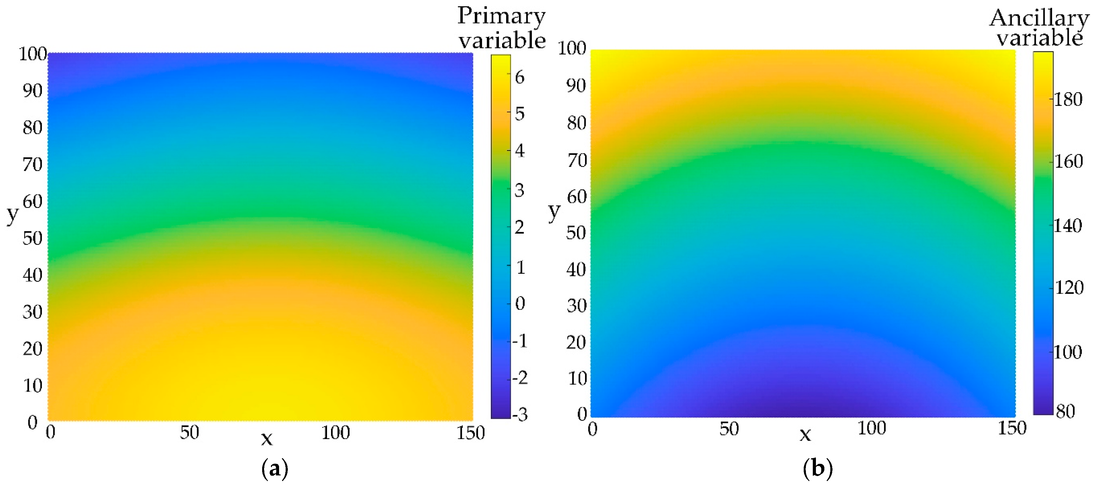
Figure 2.
Sampling points of (a) property model and (b) ancillary model.
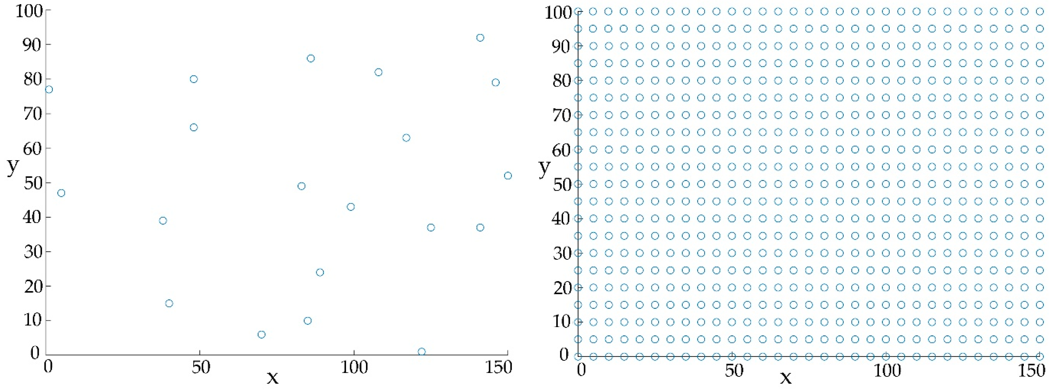

Figure 3.
(a) MRBF interpolated result, (b) scatter plot, and (c) error distribution.
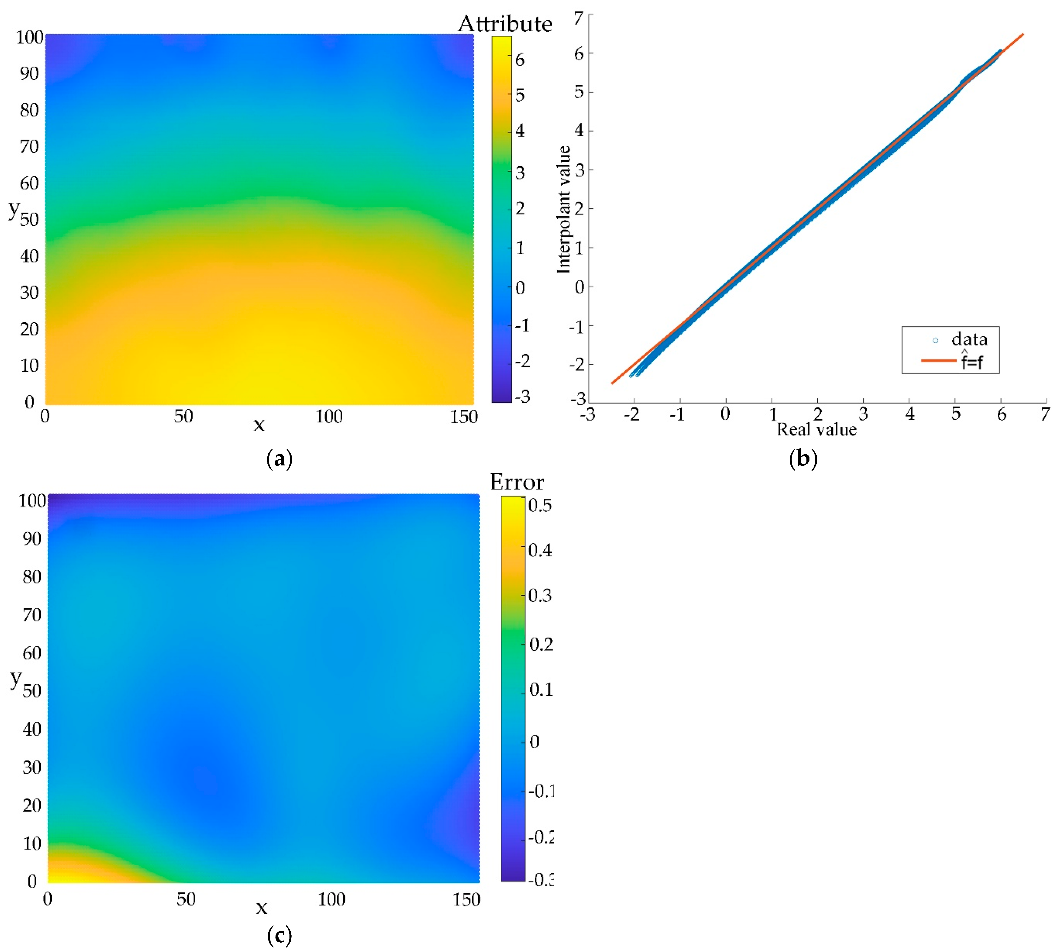
Figure 4.
Construction site’s location: (a) Hunan Province and (b) construction site.
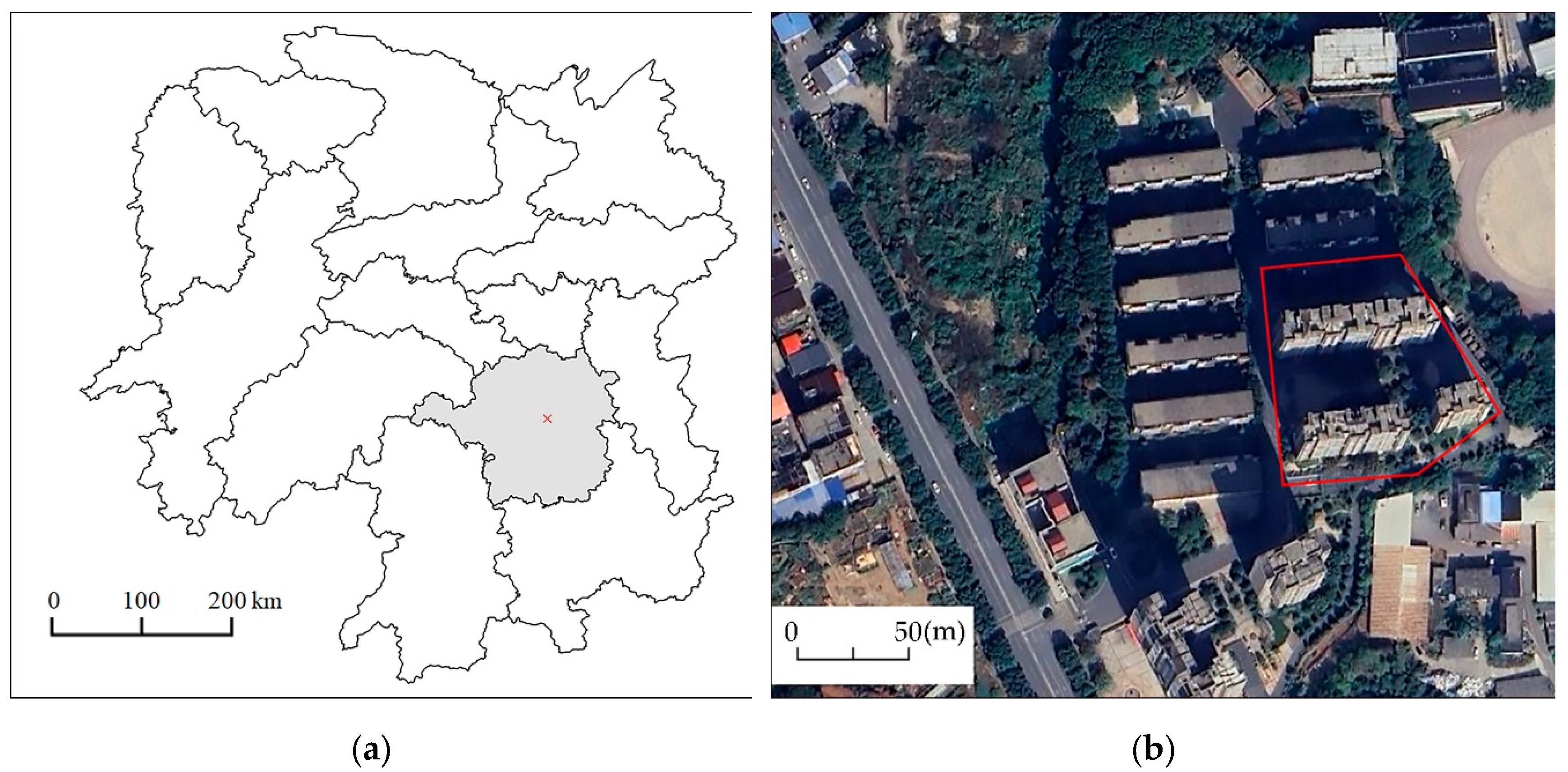
Figure 5.
Distribution of (a) boreholes and (b) engineering geological cross-sections.
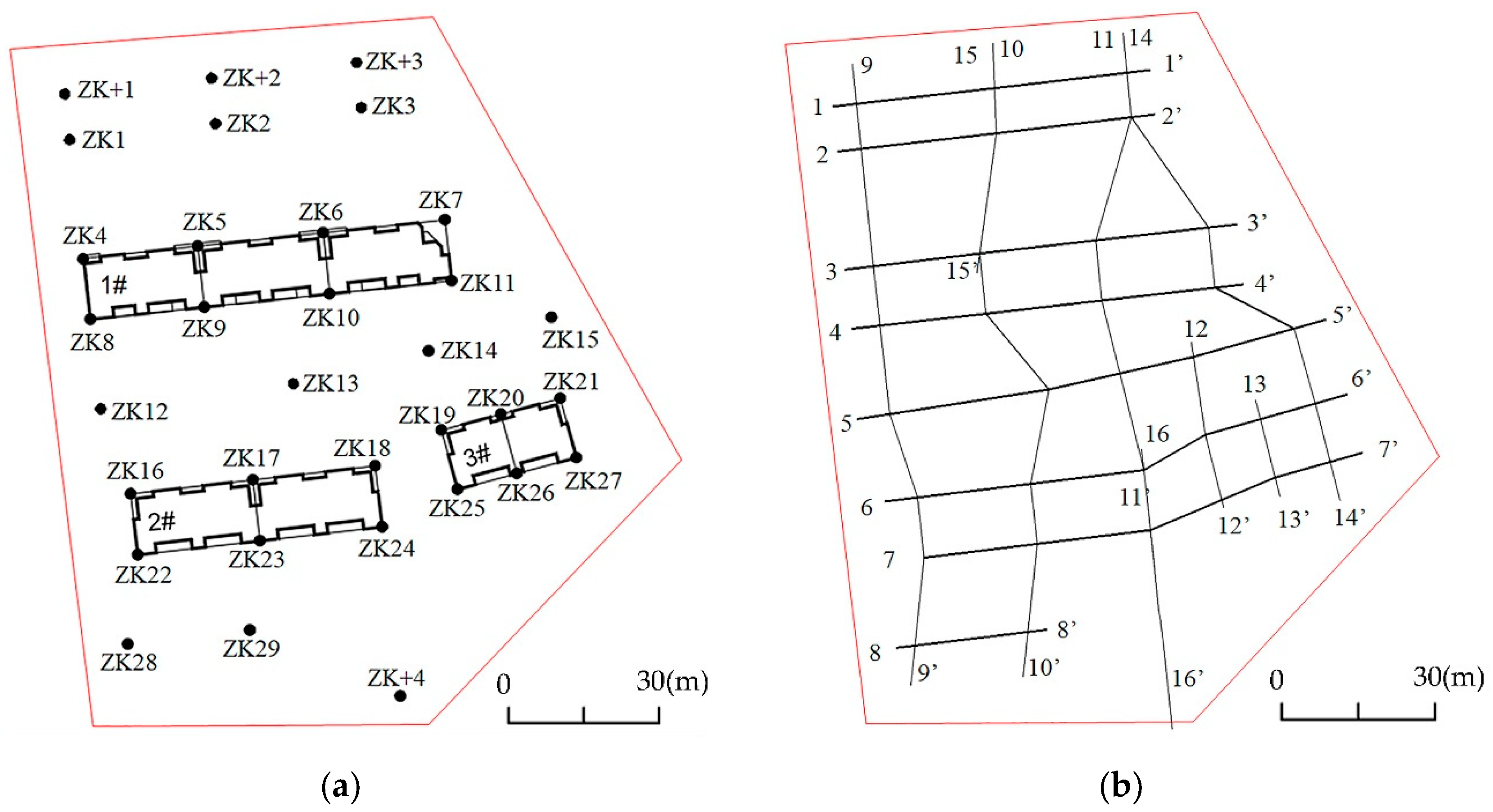
Figure 6.
Engineering geologic profile 2-2’.
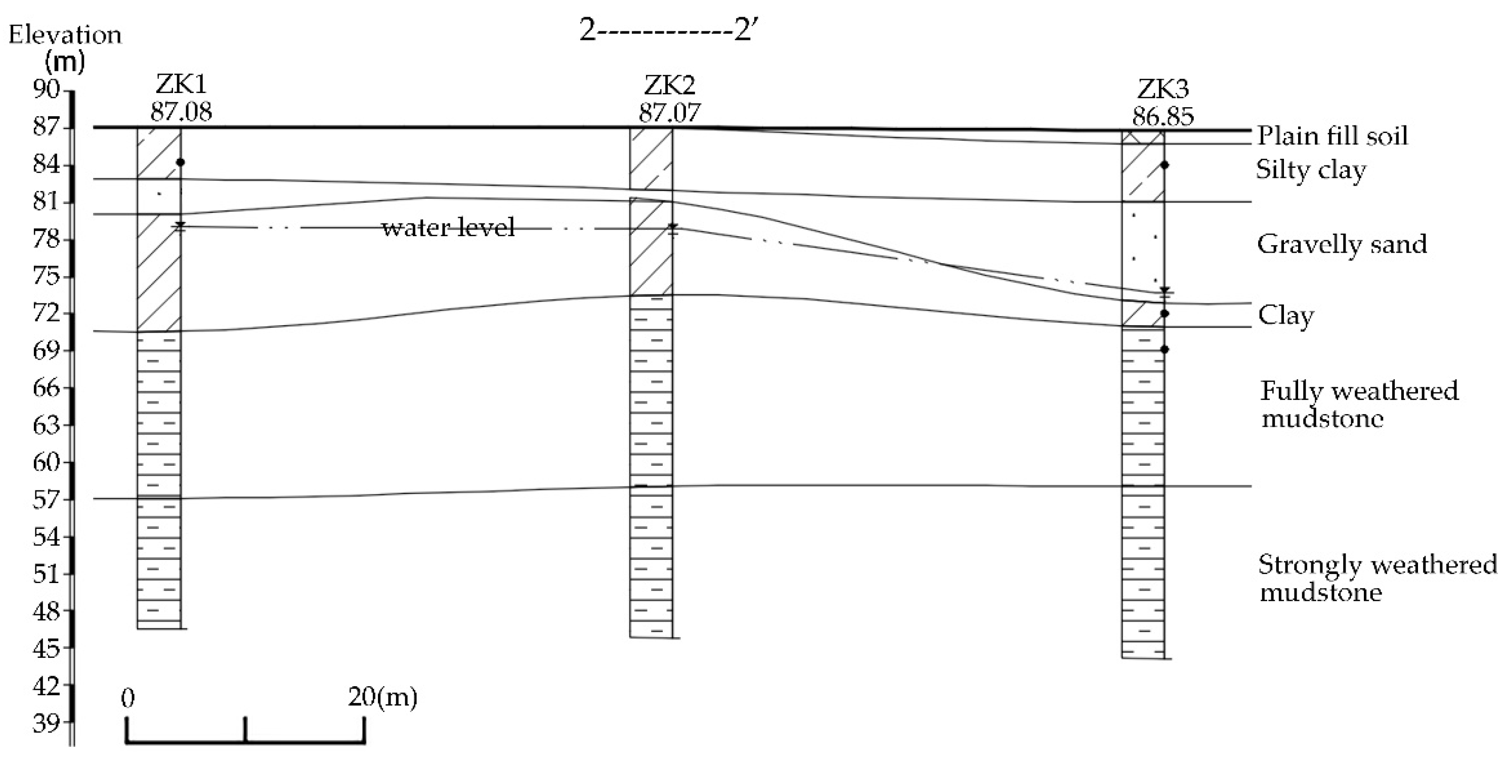
Figure 7.
Surface building model: (a) top view and (b) 3D view.
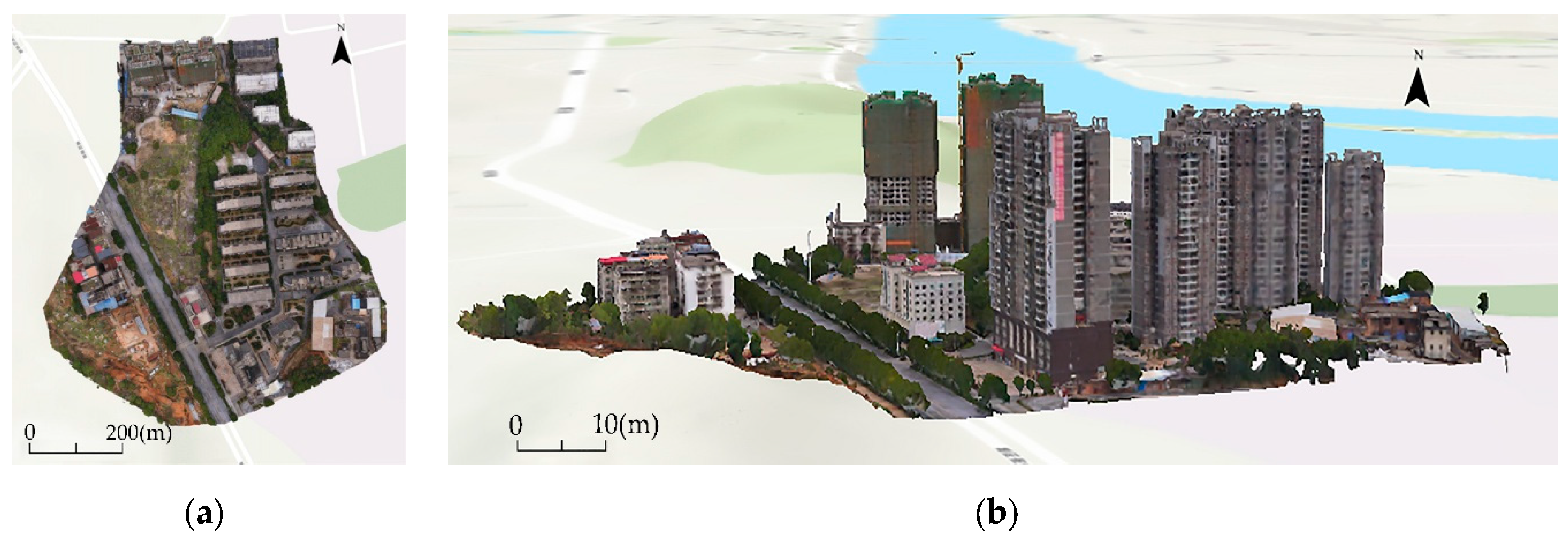
Figure 8.
Three-dimensional geological structural modeling.
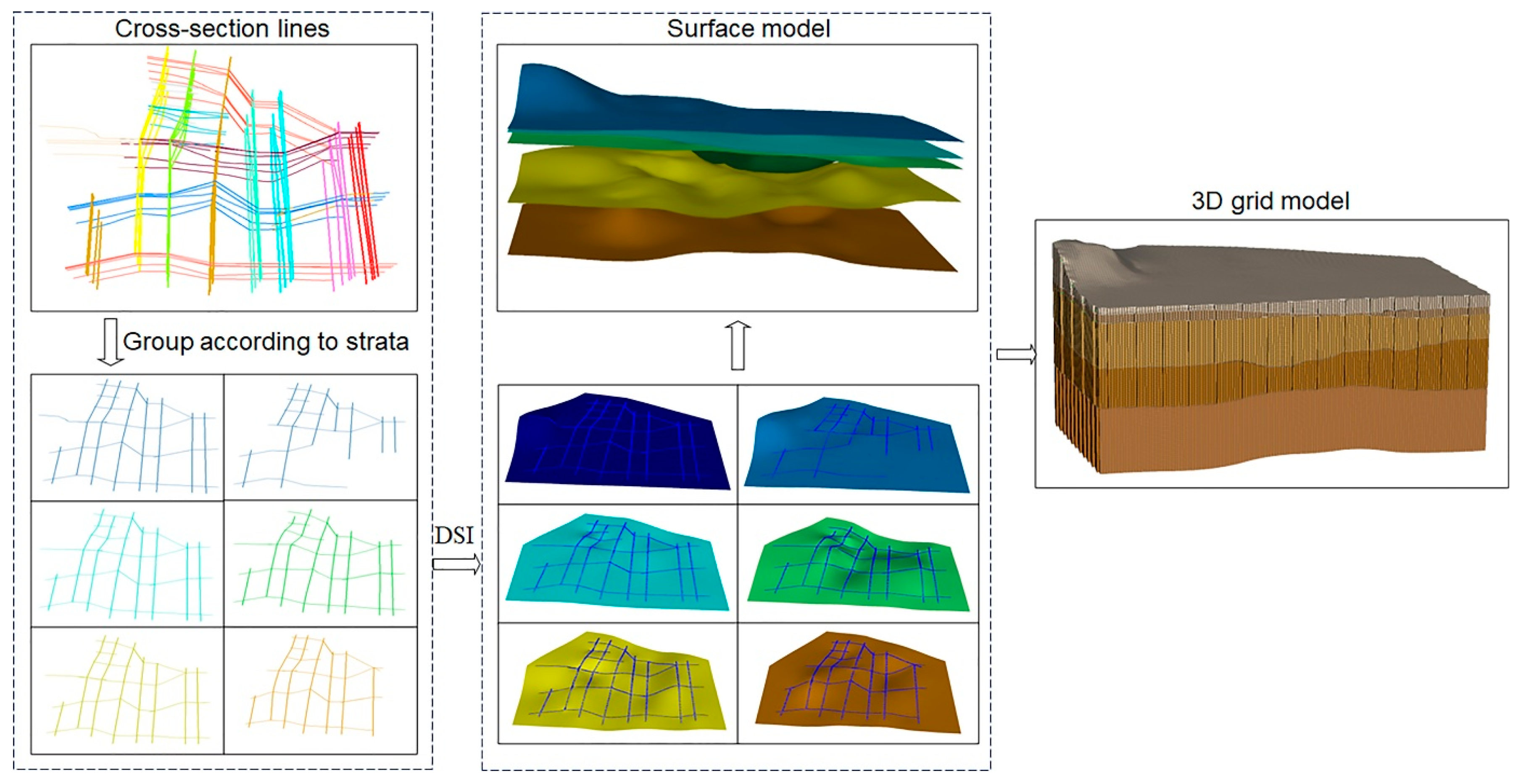
Figure 9.
(a) Groundwater level surface model and (b) the bottom surface of gravel sand layer.
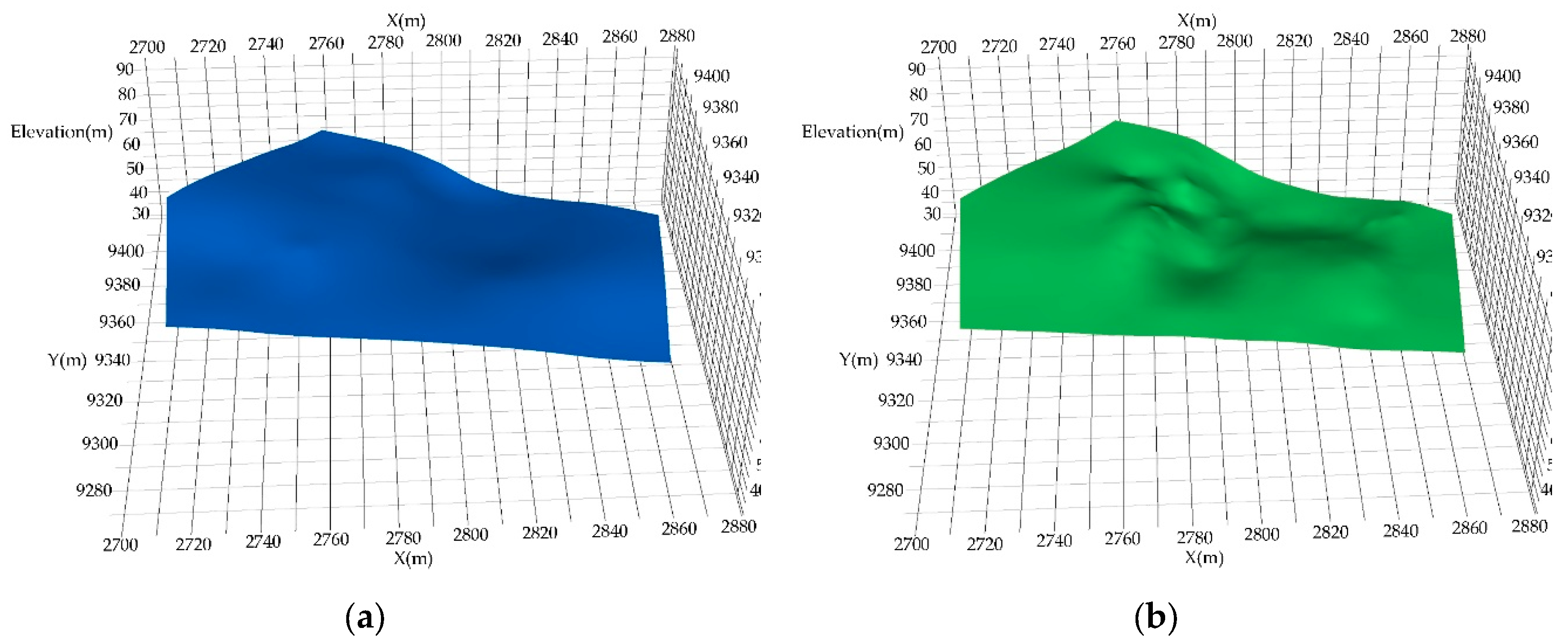
Figure 10.
Stratigraphic potential field model.
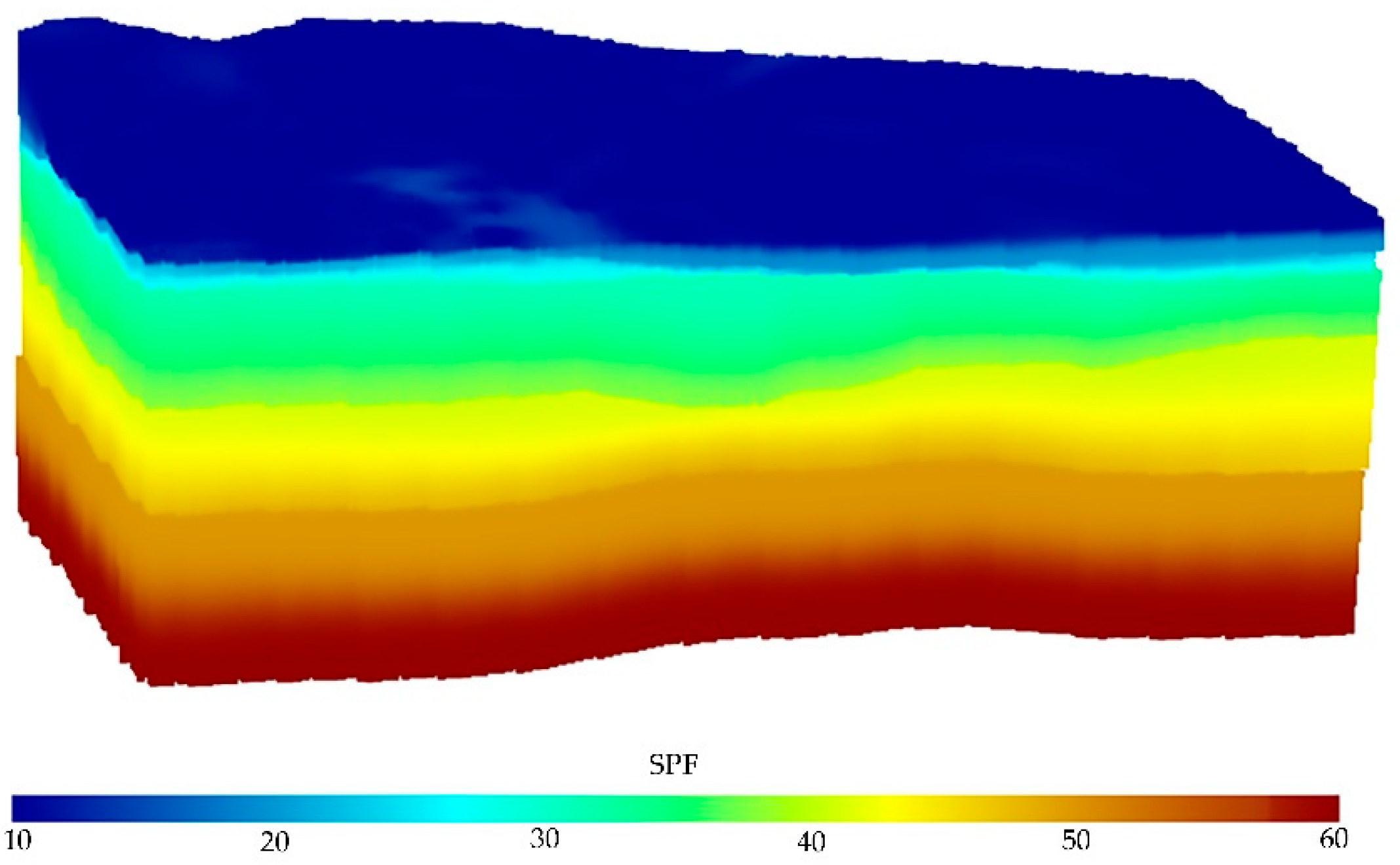
Figure 11.
Three-dimensional property models.
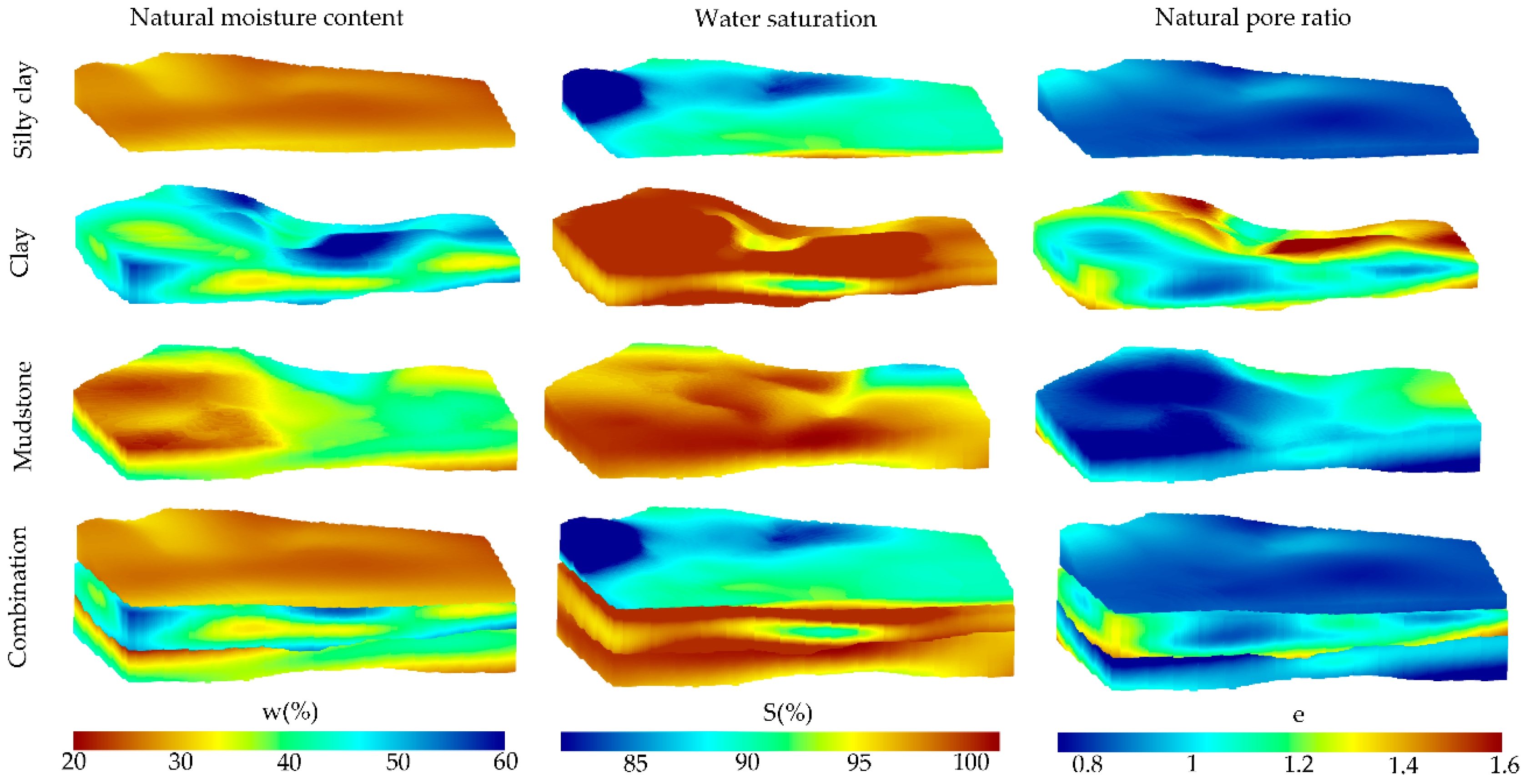
Figure 12.
Histograms of the property values of each stratum.
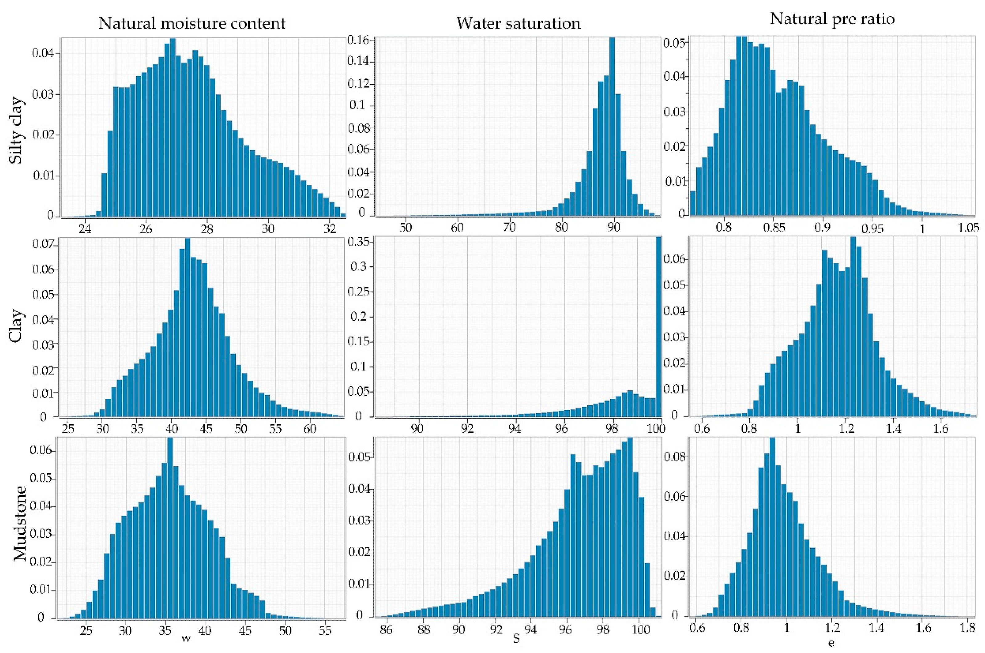
Figure 13.
(a) Distribution of pile foundations and (b) their bearing capacities.
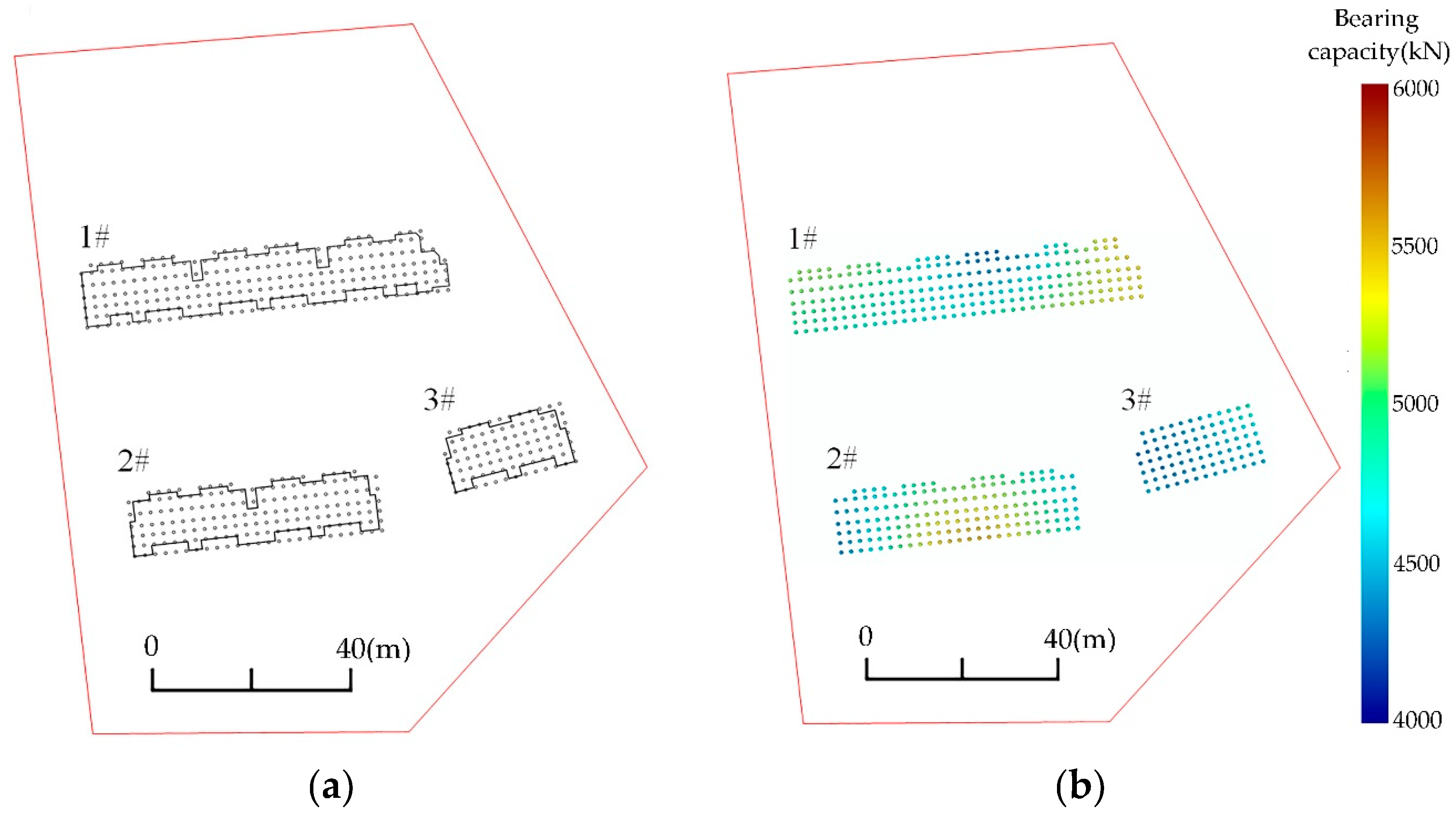
Figure 14.
Integrated surface building and subsurface engineering geological models.
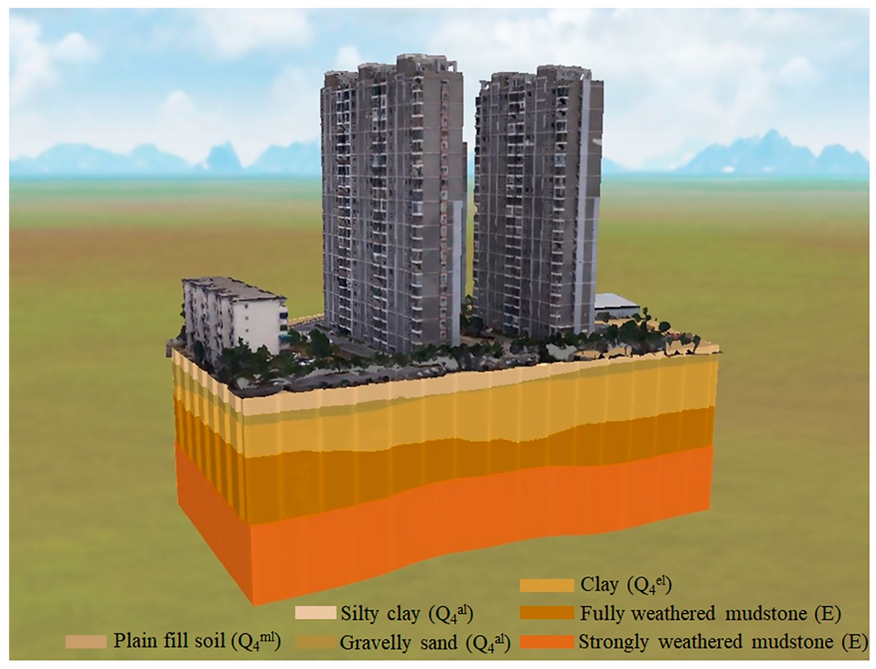

Table 1.
Volume and thickness of each stratum.
| Stratum | Volume | Average thickness | Thickness Range |
|---|---|---|---|
| Plain fill soil (Q4ml) | 10901.9 | 0.72 | 0.5 m-3.4 m |
| Silty clay (Q4al) | 54567.2 | 3.60 | 0.8 m-12.3 m |
| Gravelly sand (Q4al) | 74792.8 | 4.94 | 0.3 m-16.5 m |
| Clay (Q4el) | 135235 | 8.93 | 1.2 m-17.1 m |
| Fully weathered mudstone (E) | 170587 | 11.3 | Partially undissected, maximum control layer thickness 15.5m. |
| Strongly weathered mudstone (E) | 298465 | 20 | Largely undissected. |
Table 2.
Number of pile foundations and the bearing capacity characteristic values of each building.
Table 2.
Number of pile foundations and the bearing capacity characteristic values of each building.
| Building No. | The number of piles | The characteristic value of pile bearing capacity (kN) |
|---|---|---|
| 1# | 236 | 2162.48 |
| 2# | 166 | 2191.08 |
| 3# | 89 | 2153.81 |
Disclaimer/Publisher’s Note: The statements, opinions and data contained in all publications are solely those of the individual author(s) and contributor(s) and not of MDPI and/or the editor(s). MDPI and/or the editor(s) disclaim responsibility for any injury to people or property resulting from any ideas, methods, instructions or products referred to in the content. |
© 2024 by the authors. Licensee MDPI, Basel, Switzerland. This article is an open access article distributed under the terms and conditions of the Creative Commons Attribution (CC BY) license (http://creativecommons.org/licenses/by/4.0/).
Copyright: This open access article is published under a Creative Commons CC BY 4.0 license, which permit the free download, distribution, and reuse, provided that the author and preprint are cited in any reuse.


