
Submitted:
17 December 2024
Posted:
18 December 2024
You are already at the latest version
Abstract
This work identifies and models the inline devices in an experimental surface plasmon resonance spectroscopy setup to determine the system’s transfer function. This allows for the comparison of theoretical and experimental responses and the analysis of the dynamics of the components of an analyte placed on the sensor at the nanometer scale. The transfer functions of individual components, including the light source, polarizers, spectrometer, optical fibers, and the SPR sensor, were determined experimentally and theoretically. The theoretical model employed Planck’s law for the light source, manufacturer specifications for some components, and experimental characterization for others, such as the polarizers and optical fibers. The SPR sensor was modeled using characteristic matrix theory, incorporating the optical constants of the prism, gold film, chromium adhesive layer, and analyte. The combined transfer functions created a comprehensive model of the entire experimental system. This model successfully reproduced the experimental SPR spectrum with a similarity greater than 90%. The system’s operational range was also extended from 400-700 nm to 400-1000 nm, constrained by the signal-to-noise ratio at the spectrum’s edges. The detailed model allows accurate correction of the measured spectra, which will be essential for further analysis of nanosuspensions and molecules dissolved in liquids.
Keywords:
Modeling
; Transfer Function
; Surface Plasmon Resonance
; Kretschmann configuration
; Spectroscopy
1. Introduction
Surface plasmon resonance (SPR) is a well-established technique for the real-time detection and analysis of biomolecular interactions. Its applications span diverse fields, including molecular interaction analysis, biomarker detection, molecular imaging, electrochemical studies, and food analysis [1,2]. Recent advances have extended SPR to more complex systems, such as nanoparticles and nanomaterials [3,4]. However, accurately modeling real SPR systems remains challenging [5]. Existing models, often based on simplified assumptions and focusing primarily on the SPR sensor itself, frequently fail to adequately account for the influence of instrumental factors [6,7]. This limitation restricts their applicability to complex experimental setups. Addressing these limitations requires a comprehensive approach that considers both the underlying physical principles of SPR and the specific experimental setup configuration.
Surface plasmons (SPs) are collective oscillation modes induced by evanescent electromagnetic waves on the free-electron charge density at the interface between a metal and a dielectric medium. Plasmonic oscillations are typically initiated by the incidence of a beam of light on the surface of the metal [8]. Surface plasmon resonance spectroscopy (SPR-S) leverages this phenomenon to quantify molecular interactions occurring in a medium in contact with the metal surface [9]. A typical experimental setup, based on the Kretschmann configuration [10], employs a high refractive-index prism coated with a thin gold film, along with a light source, a polarizer, and a spectrometer (Figure 1). Incident p-polarized light at a specific angle () excites surface plasmons. Resonance occurs when the momentum of the incident light, , equals the momentum of the surface plasmons [11] described by:
where , , and are the refractive index of the prism and the complex dielectric constants for the metal and the analyte, respectively [8].
At resonance, a unique spectral signature is created for the analyte [12]. The resonance wavelength provides information about molecular interactions at the nanometer scale [5]. However, the measured spectrum is susceptible to instrumental influences, including the wavelength-dependent radiance of the light source, attenuation in optical fibers, the transmittance of the polarizer, and other optical components (e.g. lenses, collimators), and the detection efficiency of the spectrometer [5,7,13,14]. These factors can shift the observed resonance wavelength, making accurate determination challenging [5,13,14]. Accurate interpretation requires correction of the measured spectrum for these instrumental effects [14]. Current correction methods include polynomial or Lorentzian fitting [12], identifying the intensity minimum [15,16], calculating the spectral centroid [11], and compensating for the detector response of the spectrometer [7].
Although the concept of transfer function (TF) is widely utilized in electronics and control systems for modeling input-output relationships, its application to detailed modeling and spectral correction of SPR spectrometers, to the best of our knowledge, has not been previously explored in the literature. A TF quantifies how a system modifies incident light as a function of wavelength, represented in the frequency domain as , where X is the input and Y is the output [17]. This work introduces a novel approach that employs TFs to characterize and correct the spectral response of an SPR spectrometer, taking into account the individual contributions of each optical component. The total transfer function of the system is the product of the individual component TFs.
where is the total transfer function, is the transfer function of the i-th component, and is the wavelength. It is proposed that this TF-based model will accurately reproduce the experimental spectrum, thereby enabling precise correction of measured SPR spectra and facilitating improved analysis of molecular interactions.
This work presents a detailed model of a homemade SPR-S system, incorporating the transfer functions of individual components to reproduce the system’s spectral response accurately. Section 2 describes the experimental setup, and the process of determining the TF for individual components. Section 3 validates the model by comparing theoretical and experimental responses. Section 4 describes the possible noise sources affecting the TFs and mitigation strategies. Section 5 demonstrates the model’s application for correcting SPR spectra. Finally, Section 6 presents the conclusions and outlines future research directions.
2. SPR Spectrometer System: Components and Transfer Function Determination
The SPR spectroscopy system used in this work includes a light source, a polarizer, an SPR sensor, optical fibers, and a spectrometer, as shown in Figure 2. The transfer function of each component can be determined by modeling the components separately. This section describes the theoretical framework used in the SPR spectrometer system and details the method used to determine the transfer function of each element. The models evaluated for each device are detailed in the following subsections, and the most applicable models are selected based on their correlation with the experimental results. The individual transfer functions will then be combined to create a comprehensive model of the entire SPR system.
2.1. Spectrometer
The spectrometer plays a critical role in shaping the recorded spectrum because the light collected by the SPR sensor passes through its internal components, each of which has a different spectral response. Our system uses a compact spectrometer (CCS200, Thorlabs Inc., NJ) consisting of a 600 lines/mm diffraction grating and a CCD linear sensor (TCD1304DG, Toshiba). Each component contributes to the spectrometer’s overall transfer function () affecting the observed signal.
- Diffraction Grating: This device disperses incoming light according to its wavelength. The absolute efficiency, , provided by the manufacturer [18], represents its capability to diffract light toward the CCD sensor as a function of wavelength. This efficiency curve acts as the transfer function of the grating.
- CCD Sensor: The dispersed light falls onto the CCD linear sensor, which converts the incident photons into an electrical signal. Its relative responsivity curve, [19], describes the sensor’s wavelength-dependent sensitivity to light and effectively acts as its transfer function.
Figure 3.
Transfer functions of the Grating (, red dashed line) and the CCD sensor (, blue dotted line), resulting in the transfer function of the spectrometer.
Figure 3.
Transfer functions of the Grating (, red dashed line) and the CCD sensor (, blue dotted line), resulting in the transfer function of the spectrometer.
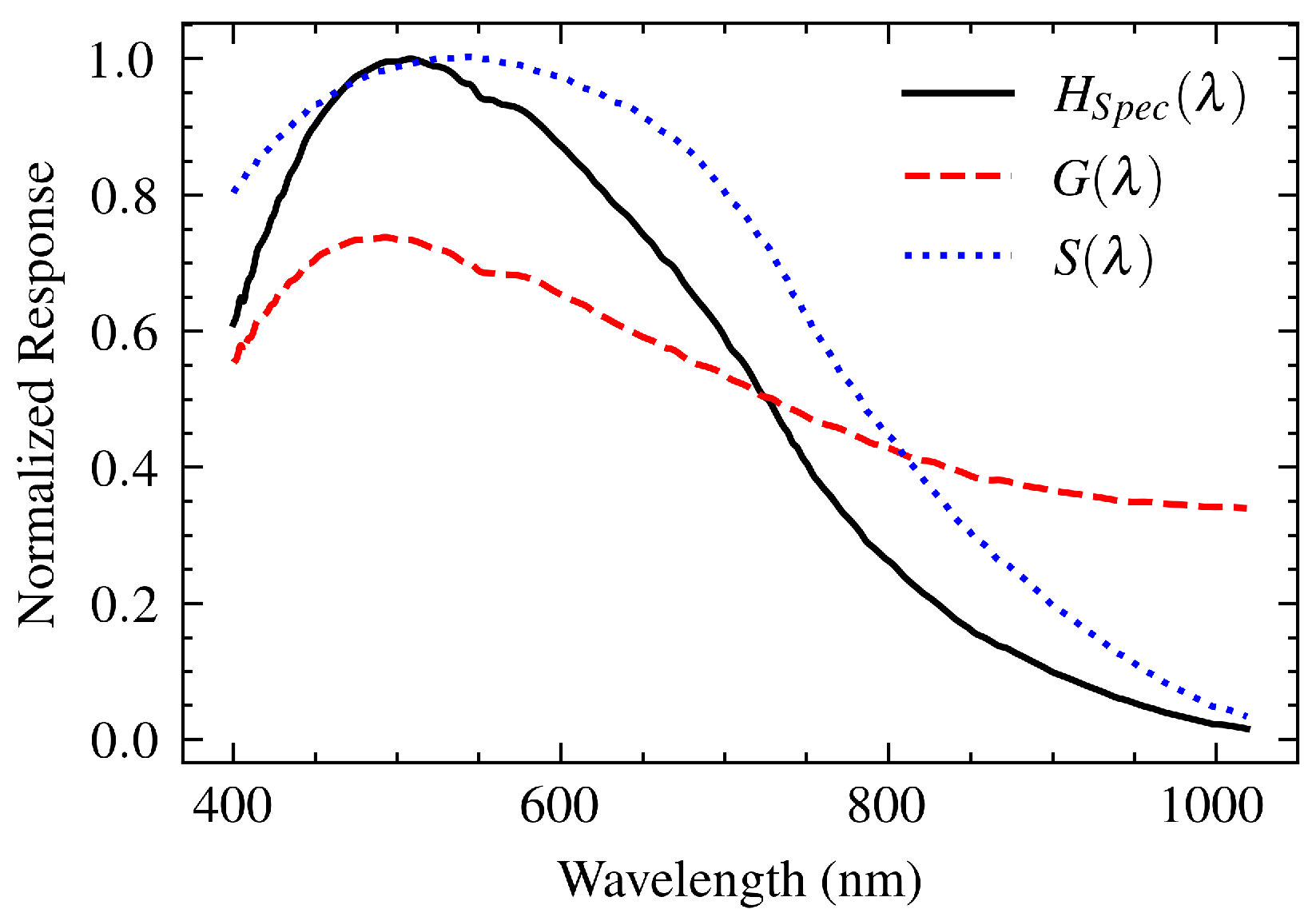
The overall transfer function of the spectrometer, , is the product of the individual transfer functions of the diffraction grating and the CCD sensor: . This product is appropriate because the light first interacts with the grating and then with the CCD; they are sequential elements in the optical path. Careful characterization of this transfer function is essential as it provides the basis for determining the transfer functions of all other components and for correcting the acquired SPR spectra.
2.2. Light Source
In the system, a stabilized tungsten-halogen lamp (SLS201L, Thorlabs Inc., NJ) is used to illuminate the gold film. The lamp’s emission spectrum, provided by the manufacturer (Figure 4, red line ) [20], is expected to follow Planck’s blackbody radiation law, which describes energy emission as a function of temperature and wavelength:
However, the recorded spectrum (Figure 4, green line) deviates from the expected profile due to the transfer function of the spectrometer (), which could affect the accuracy of the data. Fitting Planck’s law to the lamp spectrum yields an optimum blackbody temperature of 2650 K for wavelengths between 300 and 1000 nm. The fitting was performed using curve_fit from the scipy.optimize module in Python. The fit achieved a coefficient of determination of 0.9995. This fitted curve provides a theoretical model of the lamp’s performance and enables accurate spectrometer calibration.
2.3. Polarizer
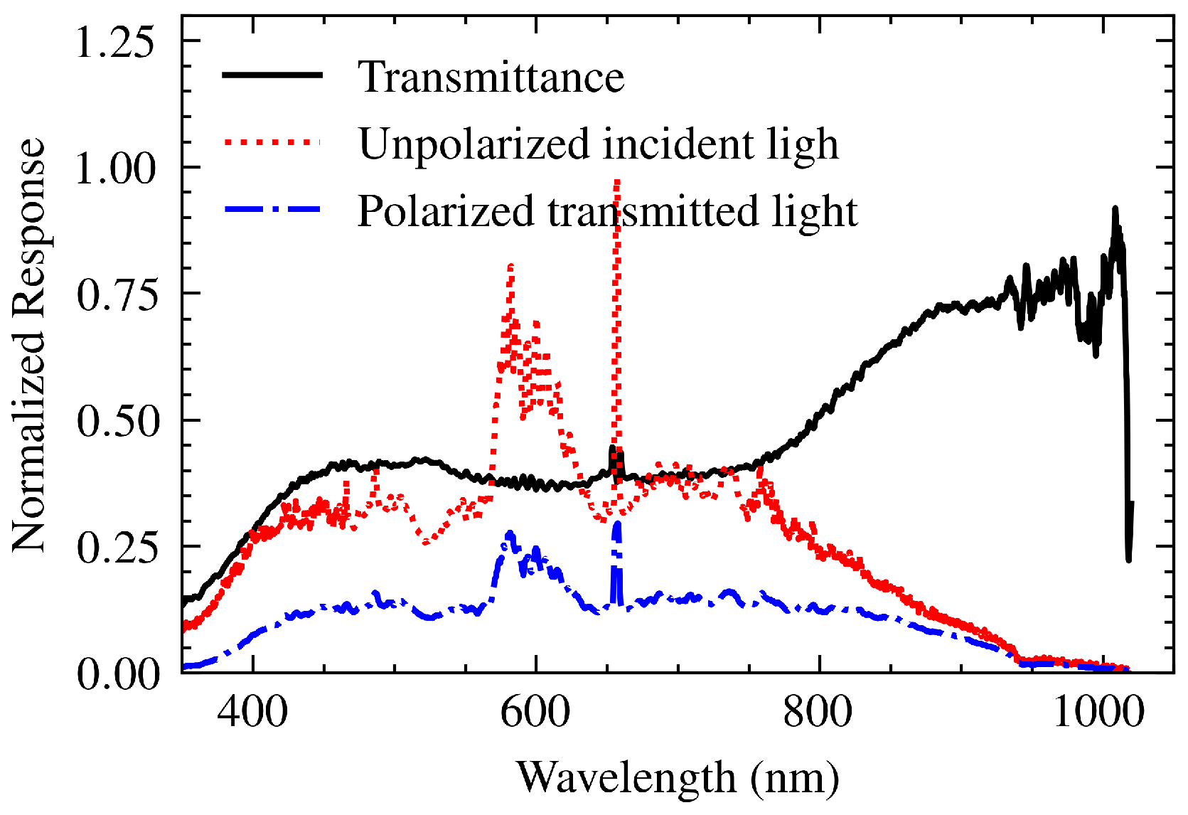
To achieve plasmon resonance, p-polarized light is required. Our experimental setup includes a polarizer [LPVISE050-A, Thorlabs Inc., NJ] to adjust the polarization of the incident light. While the manufacturer specifies its performance for wavelengths between 400 to 700 nm [21] its influence extends beyond this range. To broaden the spectral analysis, the transfer function of the polarizer, , was experimentally characterized by using a Lightsource DH-mini lamp [UV-VIS-NIR, Ocean Optics BV]. By measuring both the incident and transmitted light intensities along the polarization axis, and accounting for the TF of the spectrometer, , the polarizer’s transmittance was determined over the 350-1000 nm range. A Savitzky-Golay filter (window size = 15, polynomial order = 3) was applied to smooth the resulting curve.
Figure 5.
Experimentally determined transfer function (transmittance) of the polarizer, (solid black line), derived from the incident unpolarized light spectrum (dotted red line) and the transmitted polarized light spectrum (dash-dotted blue line).
Figure 5.
Experimentally determined transfer function (transmittance) of the polarizer, (solid black line), derived from the incident unpolarized light spectrum (dotted red line) and the transmitted polarized light spectrum (dash-dotted blue line).
2.4. SPR Sensor
The SPR sensor, based on the Kretschmann configuration, consists of an SF11 glass prism coated with a 50-nm gold film and a 0.2-nm chromium adhesive layer (HORIBA France SAS, Lyon). The reflectivity of this bimetallic structure was modeled using characteristic matrix theory [22]. This theory allows us to calculate the propagation of the electromagnetic light wave through an N-layer system, where each layer interacts directly with any other layer or optical element. Consequently, the system is modeled by a matrix product M linking every layer, represented by the matrix , sequentially in a non-commutative way, as follows
Where,
To evaluate Equation (7), it is necessary to input the optical constants of the materials that comprise the SPR sensor. Because metals absorb light, their permittivity is expressed as a complex number. The complex refractive index is defined as the square root of the dielectric constant, where the real part n is the refractive index and the imaginary part is the absorption coefficient [22]. The experimental refractive indices required for the prism [23], gold [24], chromium [25], and water [23] are shown in Figure 6. Although the refractive indices of the prism and water appear to be constant, they are, in fact, subject to slight variation within the specified spectral range. The aforementioned curves facilitate the attainment of a more precise spectral response for the sensor.
2.5. Optical Fibers
The system employs two high-quality multimode optical fibers to guide the light efficiently. The first optical fiber [P400-2-UV/VIS, Ocean Optics BV] carries the light from the source to the polarizer and then strikes the sensor. The reflected light by the sensor is then guided by the second optical fiber [FG050LGA, Thorlabs Inc., NJ] to the spectrometer.
To determine the transfer functions, it was essential to examine their attenuation spectra [26,27]. From this, the transmittance of both optical fibers was calculated using the ratio (8), which is based on the reduction of light intensity as it propagates through the fiber over a length L. The length of the optical fibers is one meter. This approach was employed to model the transfer functions and . Figure 7 illustrates, on the left, the attenuation spectra of the fibers and, on the right, their transfer functions.
2.6. Other Optical Elements
The remaining optical components used in this system, such as the prism, lens, and collimators, located along the light path, are made from highly transparent optical glasses. It is assumed that the transmittance, or transfer function, of these materials is unity within the optical spectral range, due to the negligible absorption and scattering of the materials in this region. Accordingly, a detailed characterization of these components was deemed unnecessary.
The overall transfer function of the SPR system, , is then calculated as the product of the individual transfer functions described above, as given by Equation (2) in the Introduction. This combined transfer function will be used in the next section to model and validate the complete system response against experimental measurements.
3. Experimental Modeling Validation
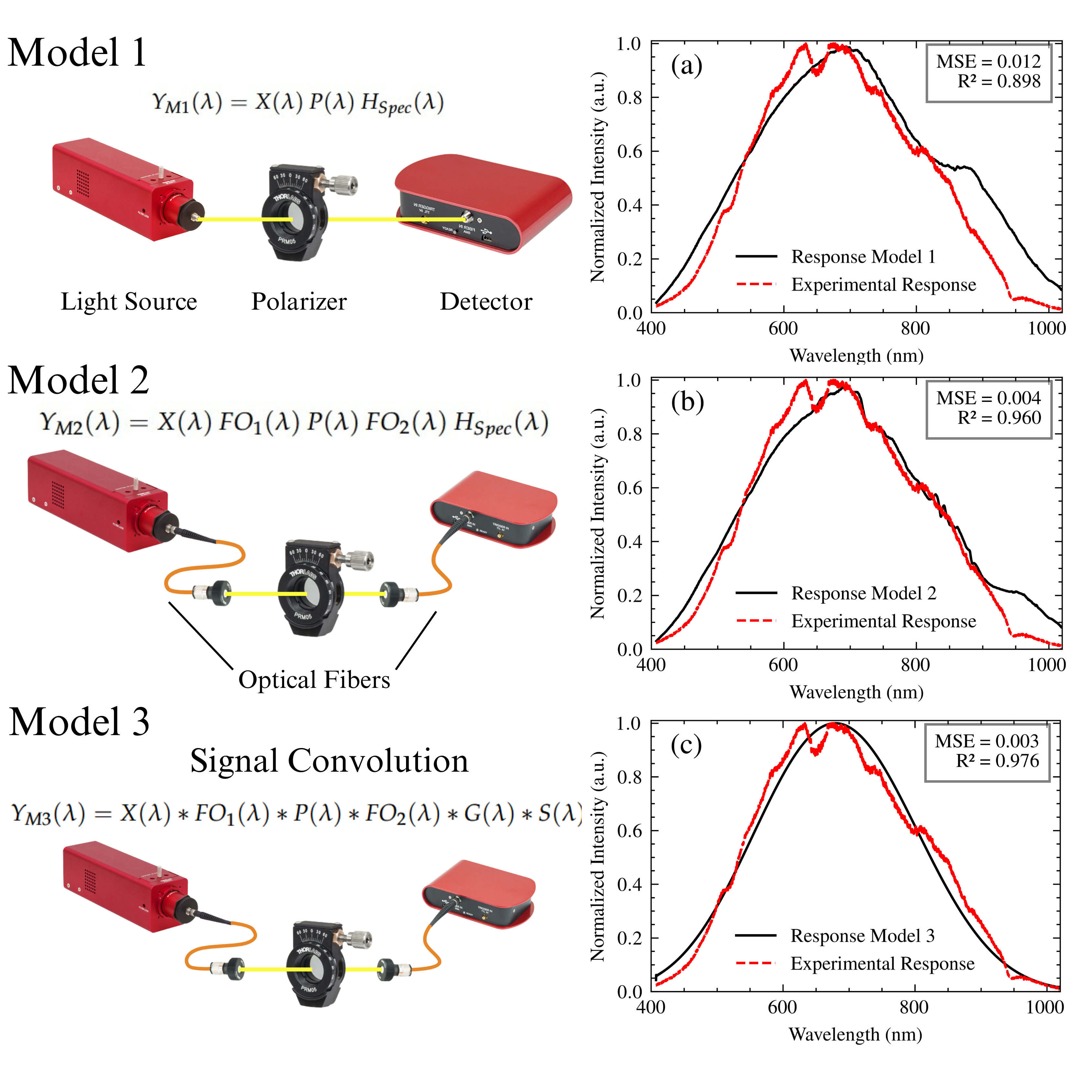
To build an accurate system model, it is essential to verify its transfer function through experimental data. This section describes the validation process, focusing on the interaction of the light source, polarizer, optical fibers, and spectrometer without the SPR sensor. This simplified approach allows for a clearer assessment of the model’s ability to reproduce the experimental spectral response and isolate the effects of these components before incorporating the more complex SPR sensor interaction. Three models of increasing complexity were developed and compared to the experimental results.
- Model 1: This model served as a baseline and assumed a negligible influence of the optical fibers employed in the setup due to their relatively short length. The overall transfer function of this model is:where is the spectral output of the light source, is the transmittance of the polarizer, and is the spectrometer’s transfer function, encompassing the effects of both the grating and the CCD sensor. This model represents a simplified scenario where the fiber’s contribution is considered minimal.
-
Model 2: This model incorporates the transfer functions associated with the optical fibers, in order to quantify the effect they have on the spectral response of the system. The complete transfer function is mathematically represented as follows:In this equation, and represent the transfer functions of the illumination and collection fibers, respectively. By integrating these elements, Model 2 accounts for the wavelength-dependent attenuation characteristic of the fibers and, at the same time, allows for a more thorough examination of the system behavior under varying conditions.
-
Model 3: The enhanced model is based on the core concepts outlined in Model 2 and includes a convolution operation to account for the combined effects of chromatic aberrations, spatial disturbances, and wavelength-dependent variations in the refractive index within the optical components. The mathematical representation of Model 3 is articulated as follows:The convolution operation provides a more realistic representation of the complex interactions between the optical elements, considering the spectral broadening and blurring effects that can occur. It accounts for how the spectral output of each component is modified and spread out by the subsequent components in the optical path. This comprehensive approach enhances the model’s ability to handle complex optical phenomena and ensures a higher accuracy in the representation of light interactions within the system.
The experimental setup for model validation consisted of a stabilized tungsten-halogen lamp (SLS201L, Thorlabs Inc., NJ) as the light source, , operating at a color temperature of 2650 K. Light from the source was coupled into a 1-meter P400-2-UV/VIS optical fiber (Ocean Optics BV), passed through the polarizer (LPVISE050-A, Thorlabs Inc., NJ), and then coupled into a 1-meter FG050LGA collection fiber (Thorlabs Inc., NJ) leading to the spectrometer (CCS200, Thorlabs Inc., NJ). The spectrometer’s integration time was set to 8 ms. The experimentally measured spectrum, , was then compared to the spectra predicted by each model. To quantify the degree of agreement between the experimental and theoretical spectra, the mean square error (MSE) and the coefficient of determination () were employed as figures of merit.
Figure 8 shows the normalized experimental spectrum and the spectra generated by the three models. Model 1, which excludes the influence of fibers, accounts for an of 0.898 and an MSE of 0.012, with discrepancies primarily at the spectral extremes. It serves to illustrate the limitations of this simplified model. Model 2, which incorporates fiber influence, significantly improved the agreement with the experimental data, achieving an of 0.960 and an MSE of 0.004. This improvement serves to confirm the importance of including the fiber transfer functions. Model 3, which incorporates a convolution operation, further refined the agreement, resulting in an of 0.976 and an MSE of 0.003. This validated Model 3 will be used in the subsequent section for correcting measured SPR spectra. The remaining discrepancies are likely within the experimental uncertainty, based on the combined effects of light source stability, low signal-to-noise ratios in regions of the spectrum, temperature fluctuations, and factors not explicitly modeled, such as dust or small imperfections in the optical components. A detailed account of the noise sources considered and the mitigation strategies employed is provided in Section 4, which resulted in low uncertainties.
4. Noise Sources and Mitigation Strategies
To obtain accurate SPR measurements, it is essential to analyze and mitigate potential noise sources that can influence the input signal and the transfer functions. This section identifies various noise sources, quantifies their impact on spectral precision, and describes the strategies employed to minimize their effects. This approach ensures precise SPR spectrum correction and reliable analyte analysis.
4.1. Noise Sources Characterization
- Light Source Fluctuations: Fluctuations in the intensity and spectral distribution in the lamp, despite using a regulated power supply, can introduce noise. The manufacturer specifies power stability below 0.05% and color temperature stability of ±15 K [20]. These fluctuations can affect the baseline stability of the SPR signal and the precision of resonance wavelength determination.
- Dark Noise: With the light source off, the spectrometer measured a normalized average intensity of . This low level, which is attributed to background noise and is unaffected by the activation of the ambient light, indicates that there are negligible contributions from dark current, electronic noise, and stray light. This verifies that the system design effectively mitigates these intrinsic sources of noise through its optical and electronic configuration
- Background Noise: With the SLS201L light source activated, the background spectrum (Figure 8, dashed red line) exhibits a maximum normalized intensity of 1 in the central spectral region, declining to approximately 3× at the edges. This restricts the precise identification of plasmonic resonances at the spectral extremes, despite a maximum signal-to-noise ratio (SNR) of approximately 333.
- Thermal Noise: It is important to note that temperature variations have the potential to impact the output of the light source and the performance of the spectrometer detector. Both exhibit a temperature sensitivity of 0.1%/C, as cited in reference [18,19,20]. The laboratory temperature is maintained at 0 degrees Celsius ± 2 degrees Celsius. The combined uncertainty in light output and detector response resulting from this ± 2 C variation is approximately 0.28%, calculated by adding the individual uncertainties in quadrature.
- Inherent Noise: Molecular vibrations within the sample itself introduce inherent noise, causing fluctuations in the local refractive index and affecting the interaction with the evanescent wave. This noise impacts both the intensity and spectral resolution of the SPR signal and is considered in the analysis.
4.2. Mitigation Strategies and their Effectiveness
- Light Source Stabilization: To mitigate light source fluctuations, a regulated power supply was used, and the lamp was allowed to warm up for 10 minutes before measurements, following IES standards [28]. During this warm-up period, the spectrometer remained operational and exposed to the light source, allowing it to reach a stable thermal and electrical state. This procedure stabilized the luminous flux, ensuring a luminous intensity variation of less than 0.05% and a power variation limited to 0.01% per hour.
- Background Noise Reduction: The system design was optimized to minimize the intrusion of stray light. In this design, the elements are positioned as closely as possible. The collection optical fiber, with a numerical aperture of 0.22, was situated at a distance of 5 mm from the prism, which served to mitigate the influence of ambient light.
- Thermal Stabilization: The SPR-S system was housed in a temperature-controlled environment (18-22 C) to minimize thermal noise and ensure stable and reliable measurements. This significantly reduced temperature-induced fluctuations in system performance.
4.3. Noise Quantification and Measurement Uncertainty
The performance of the SPR spectrometer system was evaluated by quantifying the signal-to-noise ratio (SNR) and spectral resolution. With an 8 ms integration time, the SNR exceeded 80 in the 450-900 nm range. Outside this range, the SNR decreased due to lower lamp irradiance and reduced CCD responsivity. The average resolution of the spectrometer was 0.22 nm, consistent with the manufacturer’s specifications [19]. The system sensitivity of RIU/ (Refractive Index Unit per wavelength) [3,16] enabled a refractive index resolution of RIU.
Considering all noise sources and mitigation strategies, the overall measurement uncertainty was estimated to be approximately 0.5%, calculated using the root sum square method. This uncertainty considers contributions from light source stability, background noise, and thermal variations.
5. SPR Spectrum Correction
Accurate correction of the SPR spectrum is essential for reliable analyte analysis and precise molecular interaction studies. For this purpose, SPR-S measurements were performed using ultrapure water as the analyte. Water was selected due to its well-characterized refractive index over the spectral range, ensuring a reliable reference to validate the system performance. Under these conditions, the measured SPR spectrum and the simulated spectrum were obtained, from which a spectrum correction process was performed (Figure 9.(a) ).
The experimentally measured spectrum is often distorted due to the wavelength-dependent performance of the system components, as described by their respective transfer functions. These variations can lead to deviations between the experimental spectrum and the simulated spectrum , complicating the interpretation of the resonance wavelength. To To address this, a correction function , was developed. This function incorporates the combined effects of the system transfer functions, as described in Model 3, and allows for accurate reconstruction of the SPR spectrum.
The correction function, , shown in Figure 9.(b), represents the intrinsic spectral response of the measurement system, incorporating the experimentally determined transfer functions of the light source, polarizer, optical fibers, and spectrometer. This effectively removes the system’s spectral influence from the measured data. The corrected spectrum, , is then obtained by
where M is a scaling factor to adjust the overall amplitude of the spectrum. This factor accounts for differences in integration time between the sample spectrum acquisition and the reference measurement used to determine . Applying this correction yields a spectrum that reflects the true resonance response of the SPR sensor, independent of the system’s spectral characteristics.
To validate the correction function, SPR spectroscopy measurements were performed on ultrapure water at different angles of incidence, specifically 53.1°, 57.4°, and 58.2°. The use of ultrapure water ensured no unexpected deposition on the gold substrate, guaranteeing results free from external interference. The corrected spectrum, , was compared to the theoretical spectrum, , obtained through simulations using the characteristic matrix theory described in Section 2.4. Figure 9 illustrates the results for an angle of incidence of 57.4°.
The corrected spectrum, , closely matches the simulated spectrum , with a similarity of 98.30% calculated using Pearson correlation coefficient and a mean square error of 0.002. Discrepancies are observed at the spectral extremes, which are attributed to the lower signal-to-noise ratio (SNR) in these regions due to reduced lamp irradiance and CCD response.
To quantify the agreement between the spectra, the resonance wavelength for both the corrected and simulated spectra was determined using two methods: the centroid and the minimum of the spectrum. This analysis was performed for each of the incidence angles tested (53.1°, 57.4°, and 58.2°). The percentage error between the corrected and simulated resonance wavelengths was then calculated for both the centroid and minimum methods. Table 1 summarizes these results, demonstrating that the errors between and are consistently less than 1%, with an average error of 0.4%.
The results demonstrate that the correction function effectively compensates for spectral distortions introduced by the system components, enabling accurate determination of the resonance wavelength. This correction is crucial for precise analysis of molecular interactions, ensuring the measured spectrum reflects the true optical response of the analyte.
For unknown samples, the corrected spectrum can be used to determine key properties such as refractive index or concentration, once a calibration curve has been established. Additionally, the corrected spectrum facilitates monitoring of molecular interactions within the sample, providing valuable insights into dynamic processes at the nanometer scale. Future work will focus on applying this correction function to analyze the properties of nanosuspensions and molecules dissolved in liquids.
6. Conclusions
A detailed model of the experimental response of a homemade SPR spectroscopy system has been developed. This model thoroughly analyzes individual system components, enabling the determination of their respective transfer functions. Initially, the system’s operational spectral range was limited to 400-700 nm, constrained by the characterized range of the polarizer’s transfer function. However, through the methodology presented in this work, this range has been successfully extended to 400-1000 nm, broadening the scope of spectral analysis.
Three models of increasing complexity were evaluated to capture the sequential contributions of the light source, polarizer, optical fibers, and spectrometer. Model 3, which incorporates convolution to account for chromatic aberrations and other optical effects, provided the most accurate representation of the system response, reproducing approximately 97.6% of the experimental results based on MSE and metrics. This validated model 3 will be used in future work to accurately reproduce and interpret experimental SPR spectra.
Several noise sources, including light source fluctuations, background noise, and thermal variations, were identified and mitigated. These mitigation strategies resulted in a system signal-to-noise ratio (SNR) exceeding 80 within the 450-900 nm range. The experimentally determined transfer functions also explained the increased noise levels observed outside this range, particularly at the spectral extremes where lamp irradiance and CCD responsivity are diminished.
A correction function, derived from the combined transfer functions, was implemented to accurately reconstruct SPR spectra by compensating for spectral distortions introduced by the system components. This correction ensures that measured spectra reflect the true optical response of the analyte, enabling precise determination of the resonance wavelength and facilitating reliable molecular interaction analysis. Validation using ultrapure water demonstrated a high degree of similarity (98.30%) between corrected and theoretical spectra, with errors consistently below 1%.
The routine application of this correction strategy is expected to improve the processing and interpretation of experimental SPR spectra acquired with similar systems. Furthermore, the corrected spectra can be used to determine key properties of unknown samples, such as refractive index and concentration, and to monitor molecular interactions at the nanometer scale. Future work will focus on extending the model’s applicability to more complex analyte systems, specifically nanosuspensions and molecules dissolved in liquids, and further enhancing the accuracy of SPR spectroscopy.
Author Contributions
Conceptualization, R.A. and C.C.; methodology, R.A. and A.M; software, R.A. and A.M; validation, R.A. ; formal analysis, R.A.; investigation, R.A., A.M., and C.C.; resources, R.A. and C.C.; data curation, R.A.and A.M; writing—original draft preparation, R.A.and A.M.; writing—review and editing, C.C; visualization, R.A., A.M., and C.C.; supervision, C.C. All authors have read and agreed to the published version of the manuscript.
Funding
This research received financial support for equipment from the Alexander von Humboldt Foundation, Bonn, Germany.
Institutional Review Board Statement
Not applicable.
Informed Consent Statement
Not applicable.
Data Availability Statement
All data is included in the article.
Acknowledgments
The authors express their gratitude to the members of the Mass Spectrometry and Optical Spectroscopy Group (MSOS) for their fruitful discussion.
Conflicts of Interest
The authors declare no conflicts of interest.
References
- Xu, J.; Zhang, P.; Chen, Y. Surface Plasmon Resonance Biosensors: A Review of Molecular Imaging with High Spatial Resolution. Biosensors 2024, 14, 84. [Google Scholar] [CrossRef] [PubMed]
- Ravindran, N.; Kumar, S.; CA, M.; Thirunavookarasu S, N.; CK, S. Recent advances in Surface Plasmon Resonance (SPR) biosensors for food analysis: A review. Critical Reviews in Food Science and Nutrition 2023, 63, 1055–1077. [Google Scholar] [CrossRef] [PubMed]
- Araguillin, R.; Samaniego, E.; Sarabia, I.; Santos, V.; Cattöen, X.; Hou-Boutin, Y.; Costa-Vera, C. Interactions between Plasmonic Nanoparticles with a Kretschmann-Configuration SPR Setup. In Proceedings of the 2023 International Conference on Optical MEMS and Nanophotonics (OMN) and SBFoton International Optics and Photonics Conference (SBFoton IOPC). IEEE, 2023, pp. 01–02.
- Zakirov, N.; Zhu, S.; Bruyant, A.; Lérondel, G.; Bachelot, R.; Zeng, S. Sensitivity enhancement of hybrid two-dimensional nanomaterials-based surface plasmon resonance biosensor. Biosensors 2022, 12, 810. [Google Scholar] [CrossRef] [PubMed]
- Dos Santos, P.S.; Mendes, J.P.; Dias, B.; Pérez-Juste, J.; De Almeida, J.M.; Pastoriza-Santos, I.; Coelho, L.C. Spectral analysis methods for improved resolution and sensitivity: Enhancing SPR and LSPR optical fiber sensing. Sensors 2023, 23, 1666. [Google Scholar] [CrossRef]
- Das, C.M.; Yang, F.; Yang, Z.; Liu, X.; Hoang, Q.T.; Xu, Z.; Neermunda, S.; Kong, K.V.; Ho, H.P.; Ju, L.A.; et al. Computational modeling for intelligent surface plasmon resonance sensor design and experimental schemes for real-time plasmonic biosensing: A Review. Advanced Theory and Simulations 2023, 6, 2200886. [Google Scholar] [CrossRef]
- Liu, T.; Yuan, J.; Liang, J.; Hu, S.; Hu, X.; Chen, Y.; Chen, L.; Liu, G.s.; Chen, Z.; et al. Spectral Correction Method in Spr Measurements Based on Detector Response Efficiency Compensation.
- Yesudasu, V.; Pradhan, H.S.; Pandya, R.J. Recent progress in surface plasmon resonance based sensors: A comprehensive review. Heliyon 2021, 7. [Google Scholar] [CrossRef] [PubMed]
- Prabowo, B.A.; Purwidyantri, A.; Liu, K.C. Surface plasmon resonance optical sensor: A review on light source technology. Biosensors 2018, 8, 80. [Google Scholar] [CrossRef] [PubMed]
- Kretschmann, E.; Raether, H. Notizen: Radiative decay of non radiative surface plasmons excited by light. Z. Naturforsch. A 1968, 23, 2135–2136. [Google Scholar] [CrossRef]
- Wang, G.; Shi, J.; Zhang, Q.; Wang, R.; Huang, L. Resolution enhancement of angular plasmonic biochemical sensors via optimizing centroid algorithm. Chemometrics and Intelligent Laboratory Systems 2022, 223, 104531. [Google Scholar] [CrossRef]
- Zeng, Y.; Zhou, J.; Wang, X.; Cai, Z.; Shao, Y. Wavelength-scanning surface plasmon resonance microscopy: A novel tool for real time sensing of cell-substrate interactions. Biosensors and Bioelectronics 2019, 145, 111717. [Google Scholar] [CrossRef]
- Tao, Y.; Zi-wei, L.; Chen, C.; Zhi-mei, Q. Determination of Surface Plasmon Resonance Wavelength by Combination of Radiation-Based Spectral Correction With Self-Adaptive Fitting. Spectroscopy and Spectral Analysis 2021, 41, 32–38. [Google Scholar]
- Kim, S.; Ryu, J.H.; Yang, H.; Han, K.; Kim, H.; Cho, K.; Park, S.; Hong, S.G.; Lee, K. Spectrometer-based wavelength interrogation SPR imaging via Hadamard transform. Optics Letters 2023, 48, 992–995. [Google Scholar] [CrossRef]
- Ouyang, Q.; Zeng, S.; Dinh, X.Q.; Coquet, P.; Yong, K.T. Sensitivity enhancement of MoS2 nanosheet based surface plasmon resonance biosensor. Procedia engineering 2016, 140, 134–139. [Google Scholar] [CrossRef]
- Araguillin, R.; Méndez, Á.; González, J.; Costa-Vera, Ć. Comparative evaluation of wavelength-scanning Otto and Kretschmann configurations of SPR biosensors for low analyte concentration measurement. In Proceedings of the Journal of Physics: Conference Series. IOP Publishing, 2024, Vol. 2796, p. 012009.
- Åström, K.J.; Murray, R. Feedback systems: an introduction for scientists and engineers; Princeton university press, 2021.
- Thorlabs. CCS Series Spectrometer Operation Manual, 2023. CCS200-Manual.pdf.
- Toshiba. TCD1304DG CCD LinearSensor Specifications, 2004. CCS200-MFGCCDChipSpecSheet.pdf.
- Thorlabs, Inc.. SLS201L Stabilized Tungsten Light Source User Guide. Thorlabs, Inc., rev g ed., 2024. User Guide.
- Thorlabs. Linear Polarizers: Visible (420 - 700 nm), 2024. LPVISE050-A.
- Miyazaki, C.M.; Shimizu, F.M.; Ferreira, M. Surface Plasmon Resonance (SPR) for Sensors and Biosensors. In Nanocharacterization Techniques; Elsevier, 2017; pp. 183–200.
- Polyanskiy, M.N. Refractiveindex. info database of optical constants. Scientific Data 2024, 11, 94. [Google Scholar] [CrossRef]
- Yakubovsky, D.I.; Arsenin, A.V.; Stebunov, Y.V.; Fedyanin, D.Y.; Volkov, V.S. Optical constants and structural properties of thin gold films. Optics express 2017, 25, 25574–25587. [Google Scholar] [CrossRef] [PubMed]
- Sytchkova, A.; Belosludtsev, A.; Volosevičienė, L.; Juškėnas, R.; Simniškis, R. Optical, structural and electrical properties of sputtered ultrathin chromium films. Optical Materials 2021, 121, 111530. [Google Scholar] [CrossRef]
- Thorlabs. FG050LGA Multimode Fiber, 2024. Spec Sheet https://www.thorlabs.com/drawings/167b82d7dd54993f-689E7118-FC74-4796-CBA105869799A71A/FG050LGA-SpecSheet.pdf.
- P400-2 UV-VIS Fiber for Ocean Optics Spectrometers. https://www.laserlabsource.com/Spectrometers/shop/P400-2m-UV-VIS-Fiber-Ocean-Optics, 2024. Accessed: 2024-11-21.
- Rea, M.S. IESNA Lighting Handbook: Reference and Application, 9th ed.; Illuminating Engineering Society of North America (IESNA): New York, NY, 2000.
Figure 1.
Scheme of the setup used for surface plasmon resonance spectroscopy.
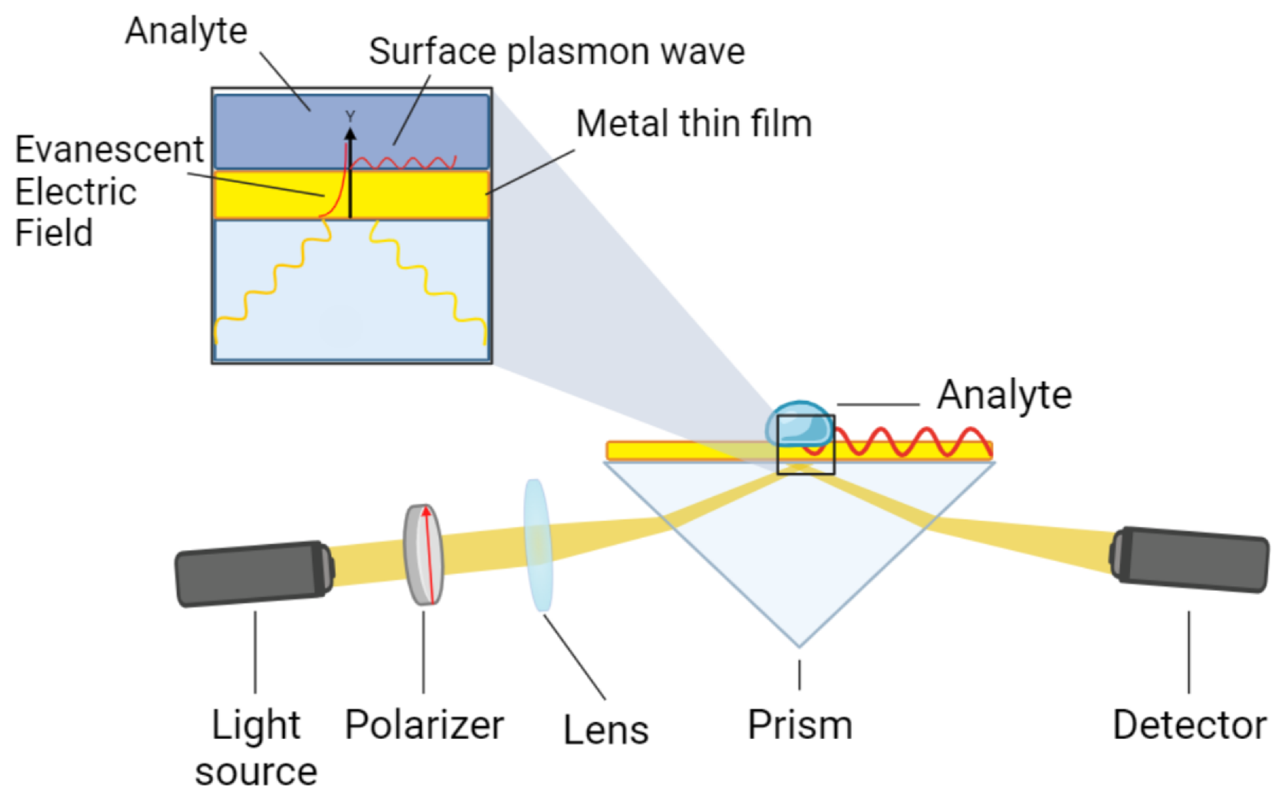
Figure 2.
Measuring system instruments arranged as in the experiment. shows the result of the interaction of light with all components of the system.
Figure 2.
Measuring system instruments arranged as in the experiment. shows the result of the interaction of light with all components of the system.
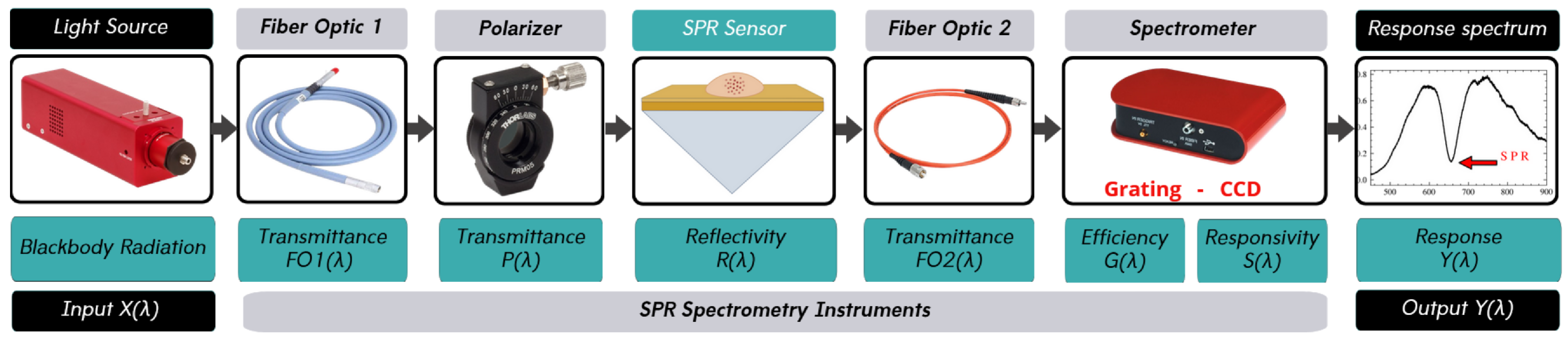
Figure 4.
Spectrum of the lamp supplied by the manufacturer (red), fitted to the radiation of a blackbody (black), and recorded by the spectrometer (green).
Figure 4.
Spectrum of the lamp supplied by the manufacturer (red), fitted to the radiation of a blackbody (black), and recorded by the spectrometer (green).
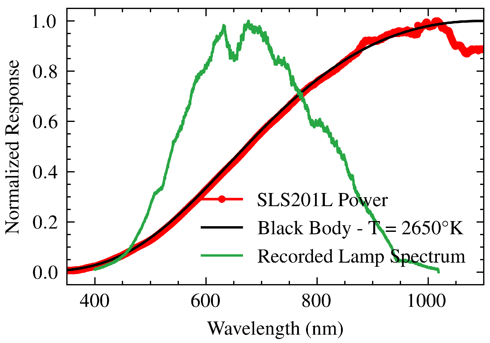
Figure 6.
Refractive index of the materials that make up the SPR sensor divided into two graphs for easy identification. (a) Refractive index curves for water and chromium film. (b) Refractive index curves for SF11 and gold film. The glass and water indexes vary rather slowly in the spectral range depicted.
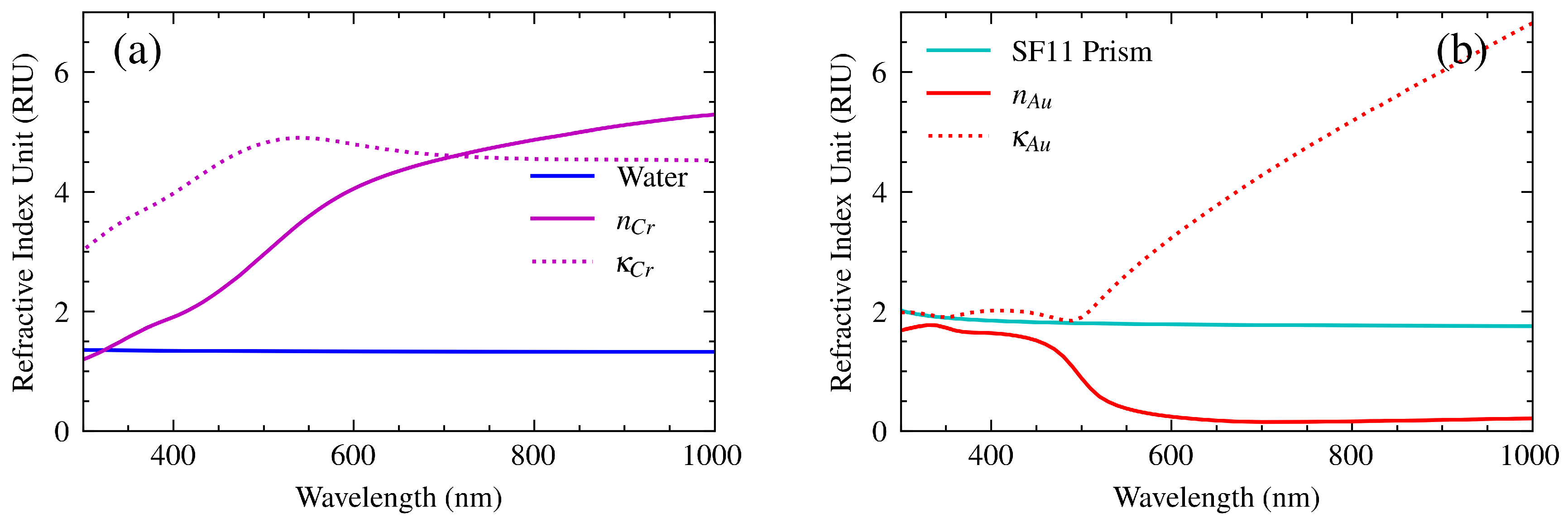
Figure 7.
(a) Attenuation and (b) transmittance (transfer functions) of the optical fibers. The solid black line represents optical fiber 1 (illumination), while the dotted red line represents optical fiber 2 (collection).
Figure 7.
(a) Attenuation and (b) transmittance (transfer functions) of the optical fibers. The solid black line represents optical fiber 1 (illumination), while the dotted red line represents optical fiber 2 (collection).
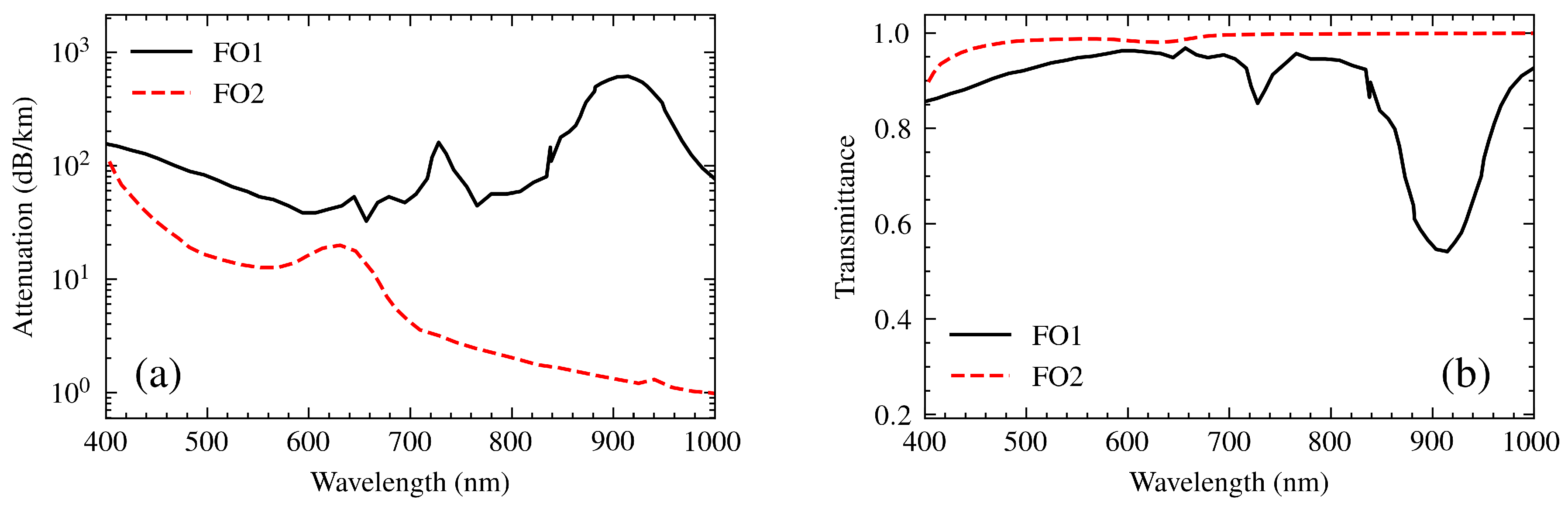
Figure 8.
Comparison of experimental and modeled spectra. Validation of the proposed models and evaluation of their performance. (a) Model 1, excludes the influence of optical fibers. (b) Model 2, includes the transfer functions of optical fibers. (c) Model 3, includes a convolution operation to represent some optical phenomena.
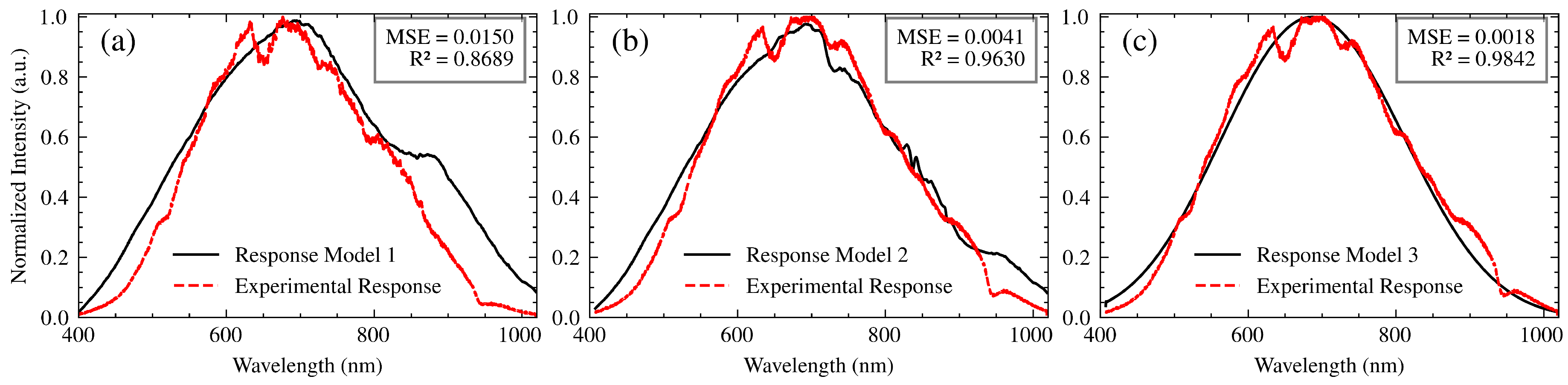
Figure 9.
Comparison of experimental, corrected, and theoretical spectra for ultrapure water at an incidence angle of 57.4°. (a) Experimental spectrum (, red line), corrected spectrum (, yellow line), and theoretical spectrum (, black dashed line). (b) Correction function, , on a logarithmic scale.
Figure 9.
Comparison of experimental, corrected, and theoretical spectra for ultrapure water at an incidence angle of 57.4°. (a) Experimental spectrum (, red line), corrected spectrum (, yellow line), and theoretical spectrum (, black dashed line). (b) Correction function, , on a logarithmic scale.
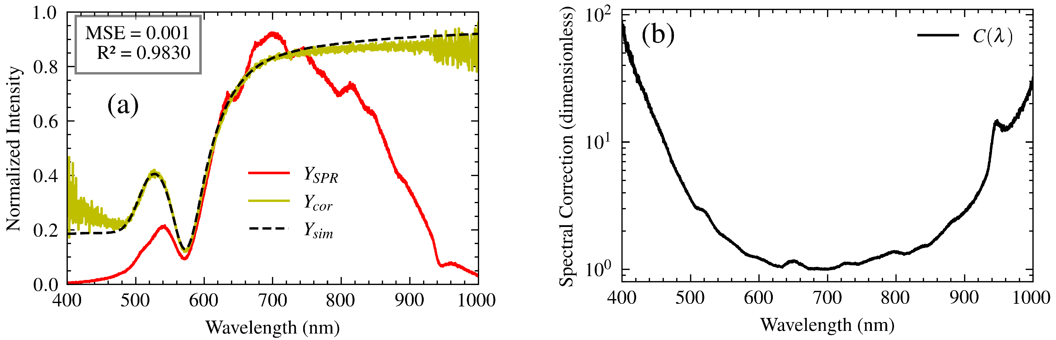

Table 1.
Results and errors obtained when purchasing corrected and simulated responses.
| θ | Y | Centroid Wavelength | Error | Minimun Wavelength | Error |
|---|---|---|---|---|---|
| 53.1° | Corrected | 663.18 | 0.45% | 658.17 | 0.30% |
| Simulated | 660.23 | 660.16 | |||
| 57.4° | Corrected | 571.88 | 0.12% | 572.88 | 0.12% |
| Simulated | 571.18 | 572.19 | |||
| 58.2° | Corrected | 559.45 | 0.66% | 559.95 | 0.87% |
| Simulated | 563.14 | 564.86 |
Disclaimer/Publisher’s Note: The statements, opinions and data contained in all publications are solely those of the individual author(s) and contributor(s) and not of MDPI and/or the editor(s). MDPI and/or the editor(s) disclaim responsibility for any injury to people or property resulting from any ideas, methods, instructions or products referred to in the content. |
© 2024 by the authors. Licensee MDPI, Basel, Switzerland. This article is an open access article distributed under the terms and conditions of the Creative Commons Attribution (CC BY) license (http://creativecommons.org/licenses/by/4.0/).
Copyright: This open access article is published under a Creative Commons CC BY 4.0 license, which permit the free download, distribution, and reuse, provided that the author and preprint are cited in any reuse.


