Submitted:
16 December 2024
Posted:
16 December 2024
You are already at the latest version
Abstract
The ship steering control to yaw motions of the marine vessels is a very frustrating assignment. Thus, this article presents the design of ship heading control system based on radial basis function neural (RBFNN) networks. The controller employs error signal and respective derivative as inputs to the RBFNN. Backward difference approximation techniques are employed to compute the error signal. Simulation results demonstrate how the control system regulates the ship heading and shows the response characteristics of the controller. The results obtained prove that the controller can perform well compared to other methods.
Keywords:
Backward Difference approximation
; ship heading control
; heading angle
; receptive field units
1. Introduction
Currently, control of ship heading has gained substantial awareness. Prodigious efforts have been dedicated to this area and remarkable outcomes have been achieved in ship autopilot design using numerous control approaches such as model reference and feedback linearization, backstepping control, fuzzy logic, sliding mode control, artificial neural networks, optimal control, adaptive control techniques and many more.
In 1911, the first vessel with automatic steering system was presented by Sperry [1]; this was followed by the proportional integral derivative (PID) based ship autopilot system proposed by Minorski in 1922 [2]. The objective of the designed autopilot systems was for course-keeping control of marine vessels. Gyoungwoo and others proposed algorithms to control a moving ship during harbor entrance [3].
A nonlinear controller design for ship autopilot based on the sliding mode control technique was proposed by Tomera [4]. The study in [4] showed that the sliding mode controller tracks better the ship’s heading irrespective of the existence of waves than the proportional derivative (PD) controller. Many dissimilar ship steering controllers have been researched basing on modern control concepts to improve the heading control.
For instance, the blend of backstepping and genetic algorithms has been applied in the design of adaptive controller for ship heading control [5]. In 2013, Perera and Soares presented an input/output linearization method by using Lyapunov and Hurwitz technique for of marine vessel steering system [6].
However, the shortcoming of a model-based technique was that the explicit knowledge dynamics are essential to be acknowledged. In recent times, to overthrow the shortcoming, Liu and others in [7] proposed adaptive fuzzy logic controller to recompense the ship navigation problems with uncertain ship’s dynamics.
Owing to the robust approximation ability, fuzzy logic system was employed to estimate unidentified nonlinear uncertainties and stimulated the advancement in ship motion control systems.
In this regard, Yang and others designed novel robust adaptive fuzzy control algorithms basing on small – gain and backstepping method [8]. Moreover, minimal learning parameter (MLP) methodology was used to lower learning parameters and computational load, which is suitable to be used in applications [9].
The backstepping technique has been used in the design of controllers for nonlinear systems from the time when it was first presented. Further in recent times, adaptive backstepping controller using dynamic surface control (DSC) has been proposed [10]. Nonetheless, the proposed controllers could not take into account the errors that emerged from filters. Providentially, a novel command filtered method was developed by Farrell and others [11].
The usage of artificial neural network in ship’s course control systems was also studied by Le [12]. In his paper, Le proposed two-multilayered feed-forward neural network ship’s course control system. The first layer plays the role of ship forward dynamics estimator and the second layer acts as a course controller. Both neural network layers are trained based on quasi-online rule using training data achieved from system’s functional process to handle the varying ship’s dynamics.
The problem for ship navigation control system with the speed loss has been presented 13]. In [13], two approaches are recommended to deal with unknown bounded disturbances for sliding mode controller employed to the surface ship heading control system. In the paper [13], the system uncertainties initiated by speed vicissitudes are treated as internal disturbances, whereas wave moments are treated as external disturbances.
Moreover, many studies have been carried out on this subject topic. Among others few literatures about heading control of ship can be obtained from [14,15,16,17,18,19,20,21,22,23,24]. Motivated by the above studies, a radial basis function neural (RBFNN) networks based controller is proposed for ship heading control. Therefore this paper aims to: presents controller design for the radial basis function neural network and examine response characteristics. Simulations are presented show how RBFNN controller regulates the ship heading. Moreover, this paper is divided into four sections: section one gives background information and literature reviews. Section two presents mathematical model of a ship heading. Section three presents the controller design. Simulations and analysis of the results are given in section four. Lastly, conclusion is given in section five.
2. Mathematical Model of the Ship
Consider a surface ship moving forward along x direction at the speed u and heading angle of ψ, and rudder input angle of δ. Let ψr be the desired heading of the ship which is specified by the pilot. The key objective is to design a controller which guarantees that ψ tracks the heading angle ψr. It is essential to ensure that best heading regulation for the ship is attained since it decreases fuel consumption. Steering performance of the ship is affected by variety of variables. It is well well-known that the ship can navigate at different speeds. At very low speed the rudder becomes less operative. Generally, a ship weighs differently on dissimilar journeys such that weighty ships turn lower. When the ship’s side is hit by wind its heading control can be affected. Similarly, ocean currents affect ship steering and hence the ship steering sensor provides the noisy measurement. Therefore, the rudder will only move between –80 and +80 degrees and this can affect the capability to steer the ship. The ship heading control problem is shown in Figure 1 below.
In order to understudy performance of a control system, a computer installed with relevant software is used to simulate the controller. To accomplish this, MATLAB codes are developed using nonlinear ship model. Usually, ship’s dynamics are derived using Newton’s laws of motion to the vessel. For very large ships, the motion in a vertical plane is disregarded for the reason that the bouncing effects of ship are minimal. Therefore the motion of ship at sea is described using coordinates fixed to the ship [25] as presented in Figure 1 above. Hence, the simplest mathematical model of the ship’s motion at sea is provided as:
where ψ and δ are the heading and rudder angles respectively. If initial conditions are set to zero, (1) becomes:
where τ1, τ2, τ3 and K are elements based on the vessel’s constant forward velocity u and length l. Principally:
Thus, for a heavy ship, τ10 = −16.91, τ20 = 0.45, τ30 = 1.43, K0 = 5.88 and l = 350m [25]. For a light ship, τ10 = −2.88, τ20 = 0.38, τ30 = 1.07, K0 = 0.83. In this paper, we use ballast conditions to simulate the ship’s performance. Similarly, we put an assumption that nominally the ship is cruising in x direction at velocity u = 5 m/s.
Normally in navigation, the vessel often creates very slight deviation from straight-line track. Hence, the (1) was derived by linearization of the equations of motion about δ = 0. Thus, the rudder angle must not surpass about 5°; or else the model will become imprecise. In this paper, we employ a model suitable for rudder angles greater than 5°; henceforth, this paper applies the model presented in [26]. The protracted model is given as:
where is a function of . The value of is established from the correlation between δ and such that. According the spiral test experiment is estimated is as:
whereand are constants and the value of. Then, we select. Similarly, it is considered that the highest aberration of the rudder angle is 80° or 80π/180 radians.
3. Design of Radial Basis Function Neural Networks Controller
This section presents the design of the RBFNN controller for ship heading regulation. The radial basis function neural network model relies on biological systems. The Radial Basis Function Neural Networks (RBFNN) contains inputs and the output is where denotes the process by the entire RBFNN. Suppose that. The input to the receptive field unit is, and its output is represented by. The receptive field unit has strength which is represented by. Suppose that there are receptive field units.
Equation (7) is the output of the RBFNN, and holds parameters of the and probably the receptive field units parameters. Also, there is another possibility how to calculate the output of the RBFNN. For example, rather than calculating the sum as in (7), thus the weighted average is calculated as follows:
The model for Radial basis function neural network is presented in Figure 2 below:
The error and its derivative are used as input to the RBFNN. Therefore, we have:
Then, employing backward difference approximation on (9) we have:
where T is the sampling period andis the index for time step. Nonetheless, in this paper we employinstead of as the argument for the signals. Now, the RBFNN for the ship is denoted as:
Thus, the RBFNN is constructed by using (10) with inputs, and, therefore we choose 121 strengths. For the we utilize (7) below to create uniform grid for thecenters,. To choose grid points, we make an assumption that lies between -90 and 90, i.e. .
where, is the scalar value, and if z is a vector, then . In case, and. Through simulation of the ship model, the turning rate of movement is always so that. Thus we make use of the assumption to support the design selections. In designing of a RBFNN for ship steering problem, we require to select parameters to form the mapping in the suitable way.
4. Simulation Study
In this section, simulation and analysis of response characteristics are presented. The simulations results indicates how the controller regulates the ship heading. To accomplish this, firstly the 3rd order nonlinear differential equations of the ship are converted into 1st order differential equations; thus, assuming
Hence, the ship model can be rewritten as:
whereand are used in simulation codes. Then, is picked such thatrelies only onandfor. Thus;
Then choosingso that does not rely on and. Choosing such that. Lastly, we choosewhich gives
Butthus
Similarly, taking. It suggests appropriate equations for simulations. Subsequently, assuming that the initial conditions be set to. This suggests that and or.For a vessel maneuvering problem, let us choose integration step size as w = 1 second and α = 10 so that T = αw = 10 seconds. The controller is simulated with a sampling period of T = 10 seconds such that a new plant input is computed every 10 seconds and used to the rudder.
If nominal conditions are used, for heavy ship, no sensor noise, no wind, and a speed maintained to 5m/s, a closed-loop responses presented in Figure 4 and Figure 5 are obtained. These results are based on the RBFNN proposed in Figure 3 of section three above. Thus, figure 4 shows that the ship’s heading ψ responds promptly, whereas some overshoots appears past the preferred value, then the response goes back to the appropriate value comparatively rapidly.
Subsequently, the effects of wind disturbances on the ship are considered. Based on this situation, the simulations result of response in figure 6 is obtained. From Figure 6, it has been noted that the wind affects the capability of the controller to attain the best steady-state regulation results of ship heading.
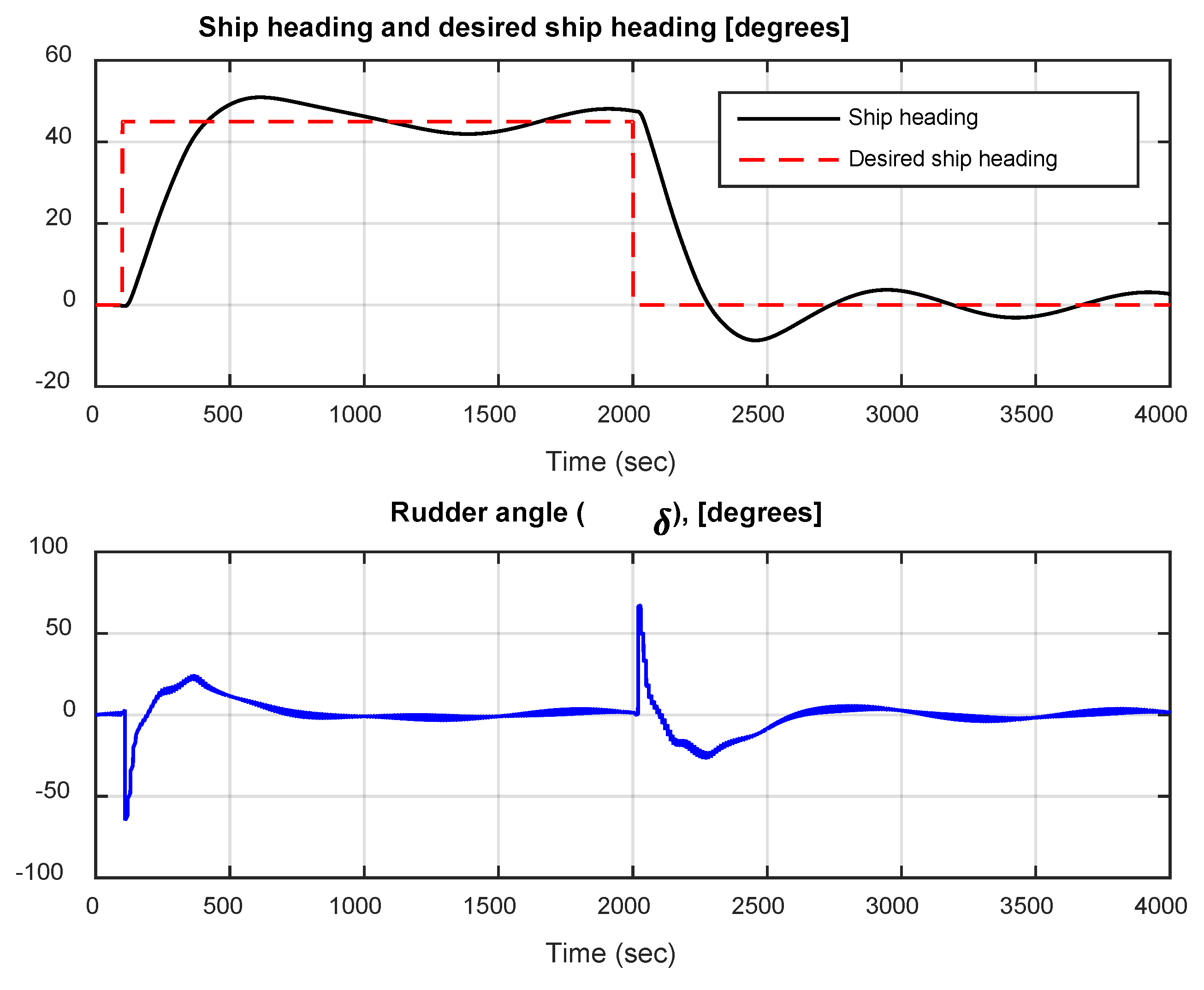
Subsequently, the influence of the speed change on capability to maneuver the ship is considered. If the speed is decreased to 3m/s, the response in Figure 7 is obtained. Figure 7, shows that the decrease in speed causes much more overshoots of the response because at this time the rudder is not effective to influence the heading of the ship.
Meanwhile, the noise sensor has small influence on the response. When change in weight occur and the ship is full, the response presented in Figure 8 is obtained. Note that there are more overshoot occurs than for nominal conditions. The reason being that, a non-heavy ship is easier to maneuver and thus the actions taken are excessively extreme and results into overshoot.
5. Conclusions
This article the design of ship heading control system based on radial basis function neural (RBFNN) networks has been presented. The error signal and respective derivative has been used as inputs to the RBFNN. Backward difference approximation techniques have been employed to compute the error signal. Simulations were carried out and the results obtained demonstrate how the control system regulates the ship heading and shows the response characteristics of the controller. The results obtained prove that the controller can perform well compared to other methods.
Author Contributions
W.E.N. and M.A.M. conceptualized, designed the RBFNN controller, ran the simulation, analyzed the results, and wrote the manuscript. P.T.N. visualized and validated the manuscript. All authors have read and agreed to the published version of the manuscript.
Funding
This research received no external funding.
Institutional Review Board Statement
Not applicable.
Informed Consent Statement
Not applicable.
Data Availability Statement
Not applicable.
Acknowledgments
I would like to Specially Thank Dar es Salaam Maritime Institute for providing facilities to accomplish of this project.
Conflicts of Interest
The authors declare no conflicts of interest.
References
- Sperry, E.A. Automatic steering. Trans. Soc. Nav. Archit. Mar. Eng. 1992, 30, 53–61. [Google Scholar]
- Minorski, N. Directional stability of automatically steered bodies. J. Am. Soc. Nav. Eng. 1922, 34, 280–309. [Google Scholar] [CrossRef]
- Gyoungwoo, L.S. , Sang-Hyun, K. Algorithms to Control the Moving ship During Harbor Entry. Appl. Math. Mod. 2009, 33, 2474–2490. [Google Scholar]
- Tomera, M. Nonlinear Controller Design of a Ship Autopilot. Intl. J. Appl. Math. Comp. Sci. 2010, 20, 271–280. [Google Scholar] [CrossRef]
- Witkowska, A. , Tomera, M., Smierzchalski, R. A backstepping approach to ship heading control. Intl. J. Appl. Math. Comp. Sci., 2007, 17, 73–85. [Google Scholar] [CrossRef]
- Perera, L.P. , Soares, G. Lyapunov and Hurwitz Based Controls for Input-Output Linearization Applied to Nonlinear Vessel Steering. Ocean Eng. 2013, 66, 58–68. [Google Scholar] [CrossRef]
- Liu, C. , Li, T.S., Chen, N.X. Adaptive fuzzy control design of ship’s autopilot with rudder dynamics. ICIC Exp. Lett. 2011, 5, 767–773. [Google Scholar]
- Yang, Y. , Feng, G., Ren, J. A combined backstepping and small-gain approach to robust adaptive fuzzy control for strict-feedback nonlinear systems. IEEE Trans. Sys. Man. Cyber. Part A: Systems and Humans 2004, 34, 406–420. [Google Scholar] [CrossRef]
- Li, T. , Li, R., Li, J. Decentralized adaptive neural control of nonlinear interconnected large-scale systems with unknown time delays and input saturation. Neurocomputting 2011, 4, 2277–2283. [Google Scholar] [CrossRef]
- Li, T.S. , Wang, D. , Li, W. A novel adaptive NN control for a class of strict feedback nonlinear systems. In Proceedings of American Control Conference, St. Louis, MO, USA, 10-12 June 2009. [Google Scholar]
- Farrell, J.A. , Polycarpou, M. Sharma, M. Dong, W. Command filtered backstepping. IEEE Trans. Aut. Contr. 2009, 54, 1391–1395. [Google Scholar] [CrossRef]
- Le, T.T. Ship heading control system using neural network. J. Mar. Sci. Technol. 2021, 26, 963–972. [Google Scholar] [CrossRef]
- Liu, Z. , Lu, X., Gao, D. Ship Heading Control with Speed Keeping via a Nonlinear Disturbance Observer. The J. Nav. 2019, 72, 1–18. [Google Scholar]
- Liu, Y. , Liu, S., Wang, N. Fully-tuned fuzzy neural network based robust adaptive tracking control of unmanned underwater vehicle with thruster dynamics. Neurocomputting 2016, 196, 1–13. [Google Scholar] [CrossRef]
- Jia, F. , & Chen, M. (2019). Design of A Nonlinear Heading Control System for Ocean Going Ships Based on Backstepping Technique. J. Coastal Res. 2019, 94, 515–519. [Google Scholar]
- Guan, W. , Zhou, H., Zuozing, S. et al. Ship steering control based on quantum neural network. Hindawi Complexity.
- Wang, R. , Deng, H., Miao, K. et al. Backstepping based integral sliding mode control with neural network for ship steering control. MATEC Web Conf 2017.
- Wang, R. , Li, D., Miao, K. Optimized radial basis function neural network based intelligent control algorithm of unmanned surface vehicles. J. Mar. Sci Eng. 2020, 8, 210. [Google Scholar] [CrossRef]
- Haouari, F. , Gouri, R., Bali, N. et al. Performance optimization of ship course via artificial neural network and command filtered CDM-Backstepping controller. Technol. Eng. 2019, 16, 5–10. [Google Scholar]
- Zhang, G. , Chu, S., Zhang, W. Composite neural learning fault-tolerant control for underactuated vehicles with event-triggered input. IEEE Trans. Cybern. 2020, 51, 2327–2338. [Google Scholar] [CrossRef]
- Zhang, G. , Yao, M., Junhao, X., Zhang, W. Robust neural event-triggered control for dynamic positioning ships with actuator faults. Ocean Eng, 2020; 207. [Google Scholar]
- Wang, W. , Liu, C. An efficient ship autopilot design using observer based model predictive control. J. Eng. Mar. Environ. 2021, 235, 203–212. [Google Scholar]
- Wang, Y. , Chai, S., Nguyen, H.D. Experimental and numerical study of ship autopilot using Extended Kalman Filter trained neural networks for surface vessels. Int. J. Naval Arch. Ocean Eng. 2020, 12, 314–324. [Google Scholar] [CrossRef]
- Wang, Y. Intelligent control for surface vessels based on Kalman Filter trained Radian Basic Function Neural Networks, University of Tasmania.
- ˚Astrom, K.J., Wittenmark, B. Adaptive Control. Addison-Wesley, Reading, MA, 2008.
- Liu, Z. , Lu, X. , & Gao, D. Ship Heading Control with Speed Keeping via a Nonlinear Disturbance Observer. J. Nav. 2019, 72, 1035–1052. [Google Scholar]
Figure 1.
Ship maneuvering problem.
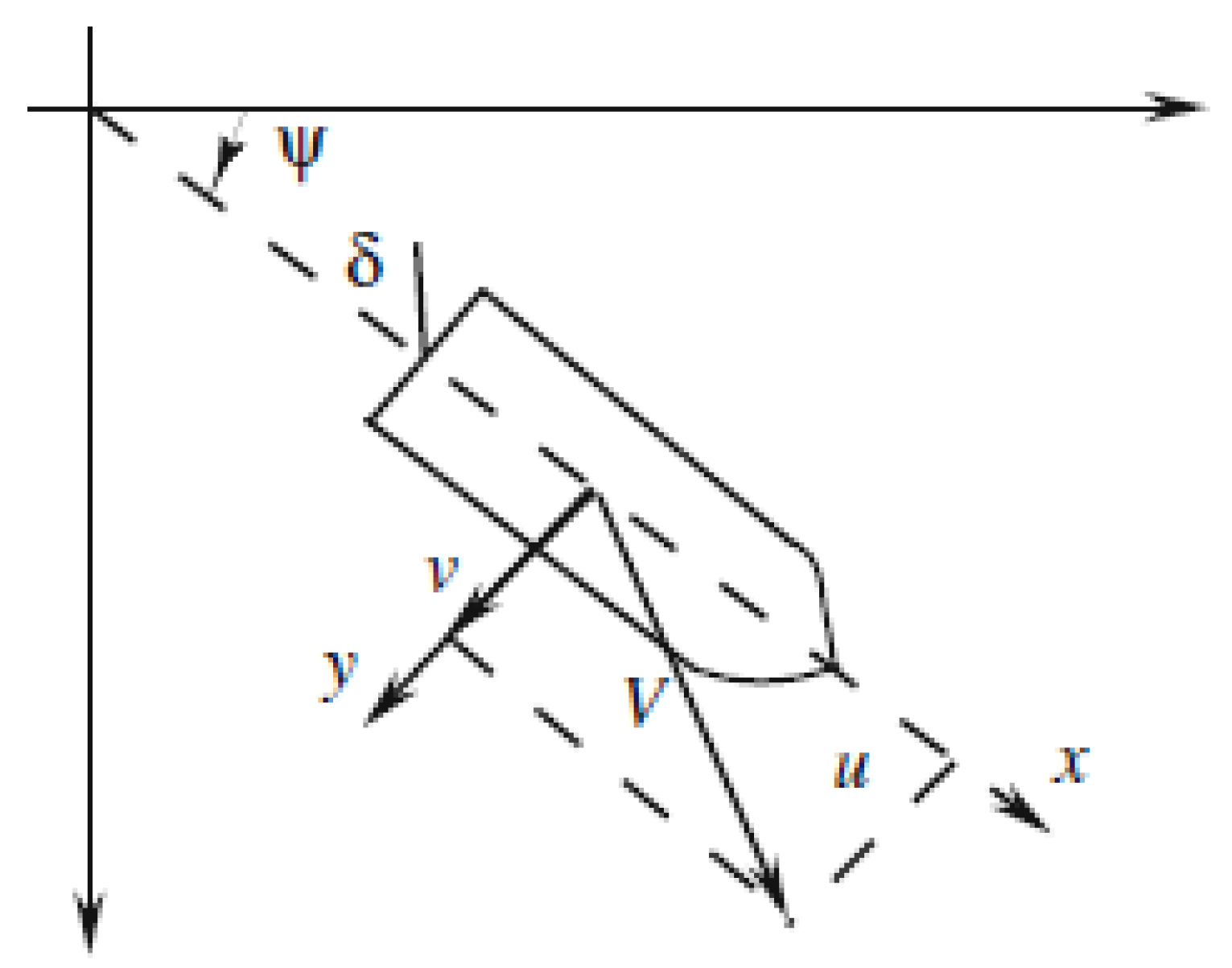
Figure 2.
Model for radial basis function neural network.
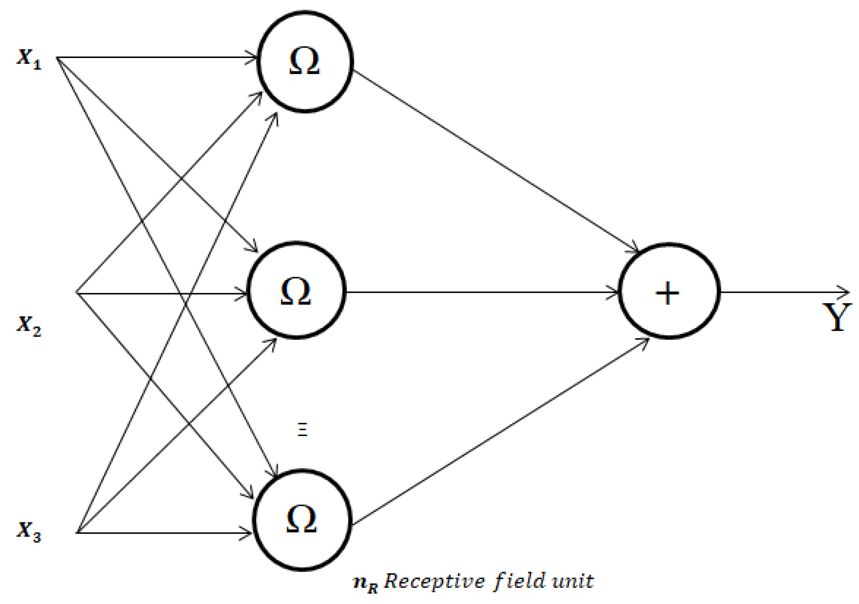
Figure 3.
Radial Bias Function Neural Network Controller.
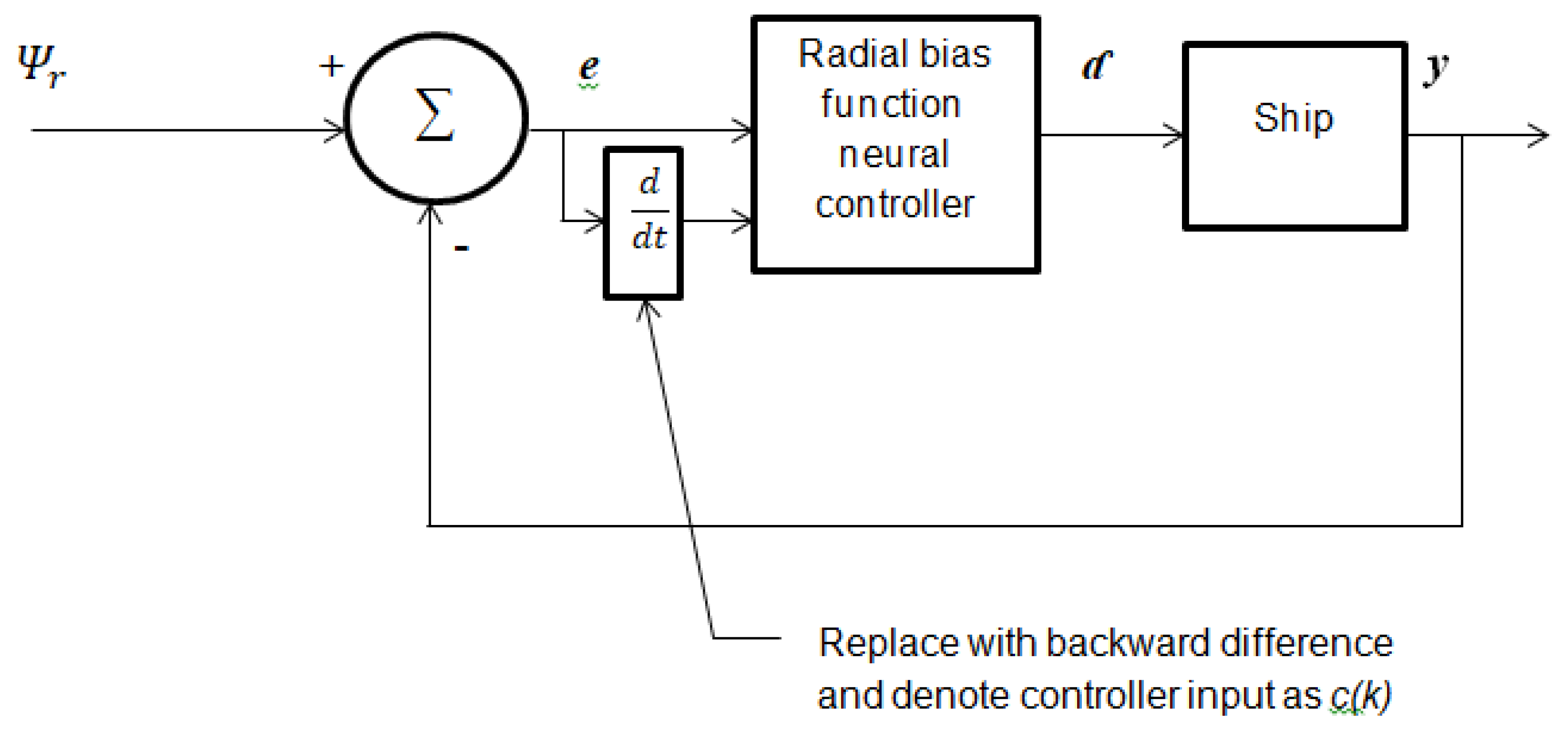
Figure 4.
A closed-loop response of the RBFNN for ship steering in absence of environmental disturbances.
Figure 4.
A closed-loop response of the RBFNN for ship steering in absence of environmental disturbances.
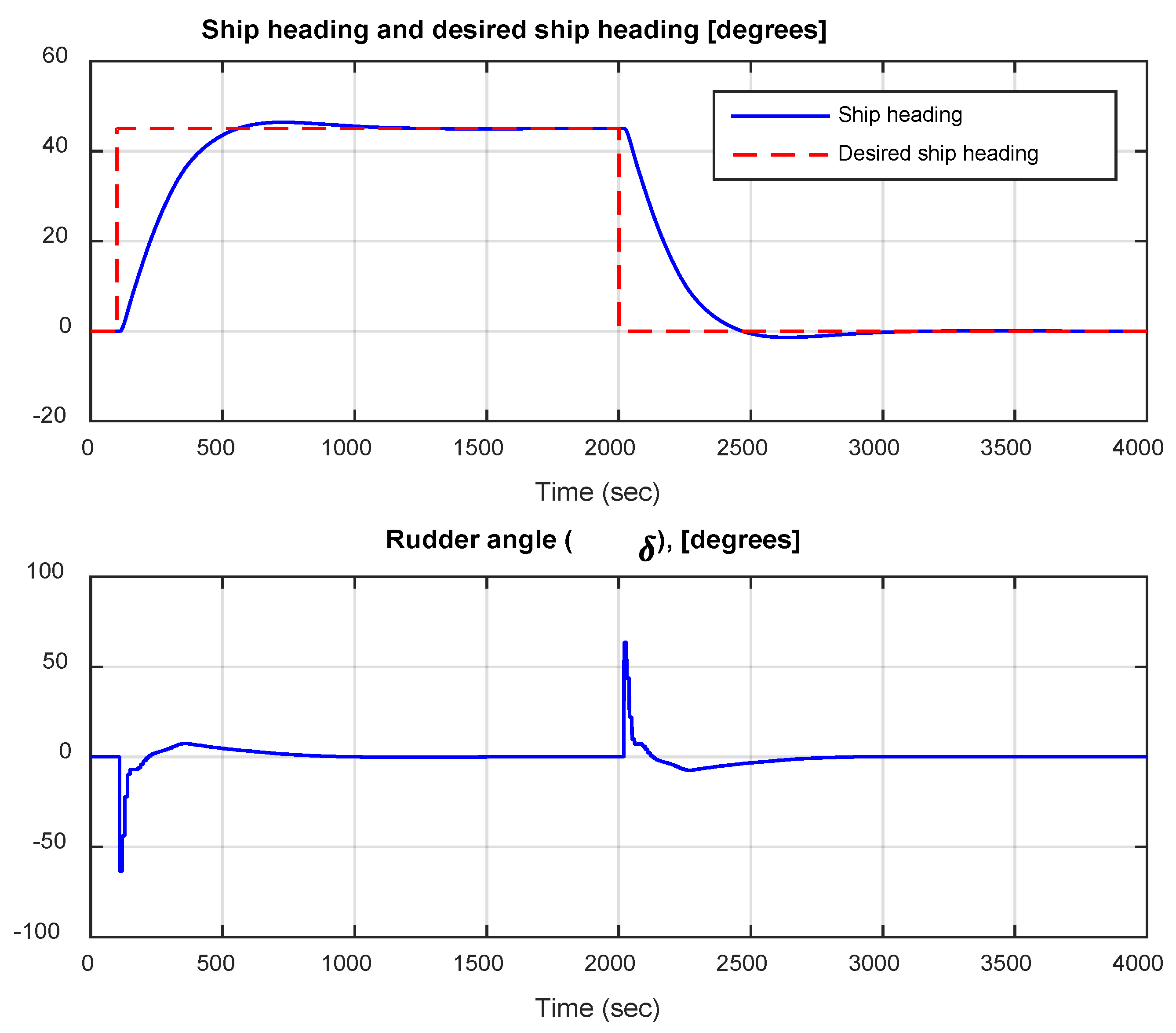
Figure 5.
A closed-loop response of the RBFNN for ship heading error steering in absence of environmental disturbances.
Figure 5.
A closed-loop response of the RBFNN for ship heading error steering in absence of environmental disturbances.
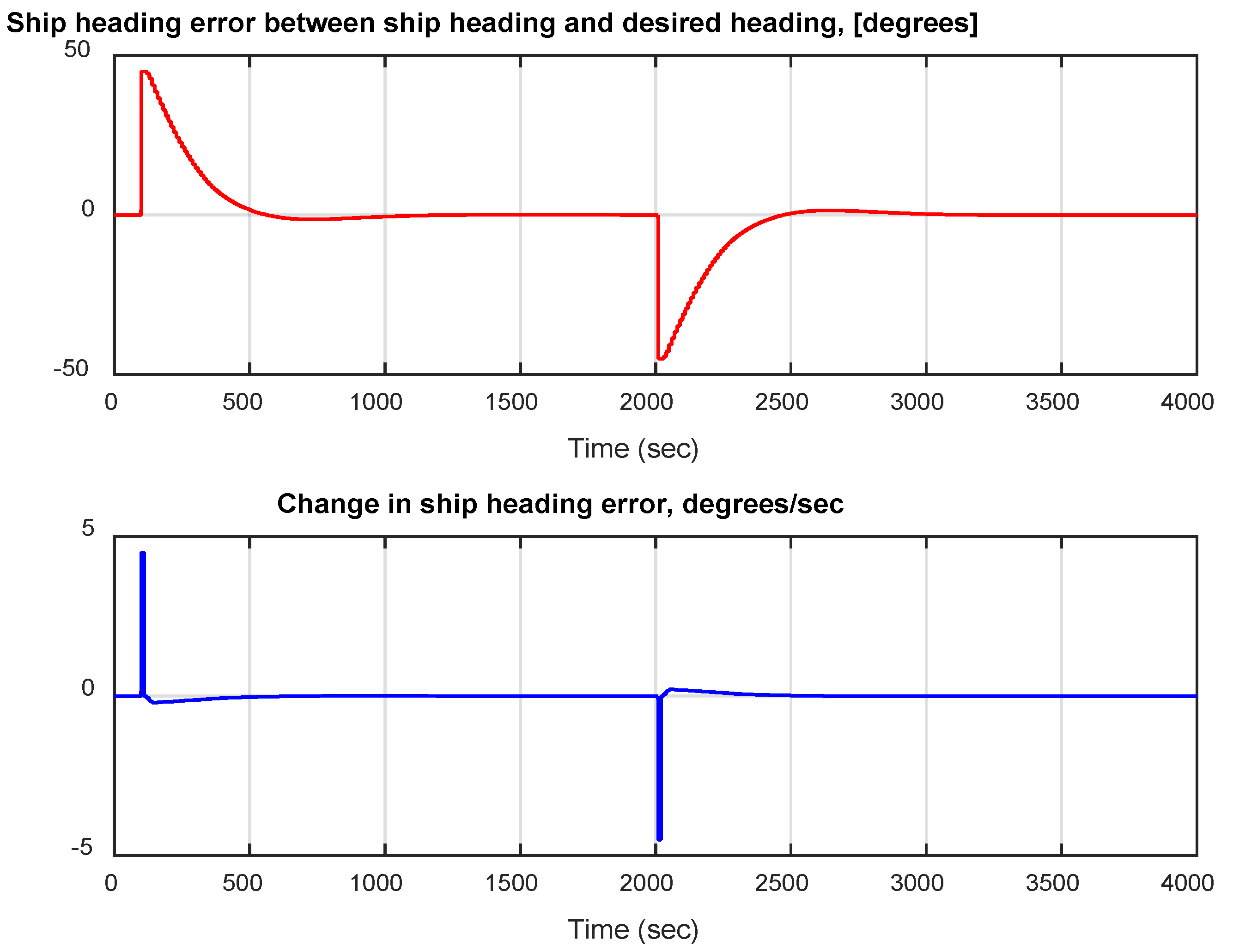
Figure 6.
A closed-loop response of the RBFNN for ship steering in presence of wind disturbance.
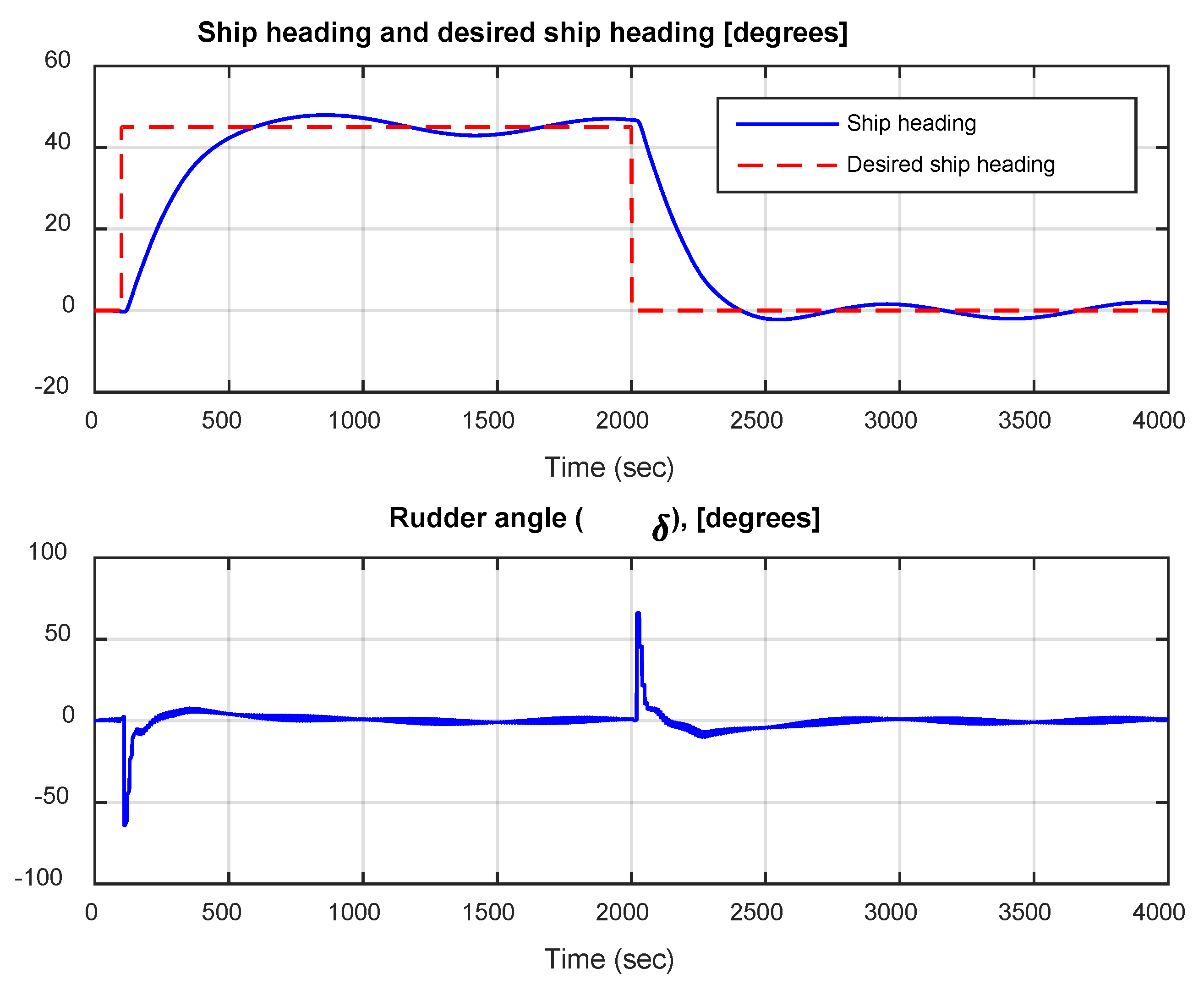
Figure 7.
A closed-loop response of RBFNN for ship steering at a speed of 3m/s.
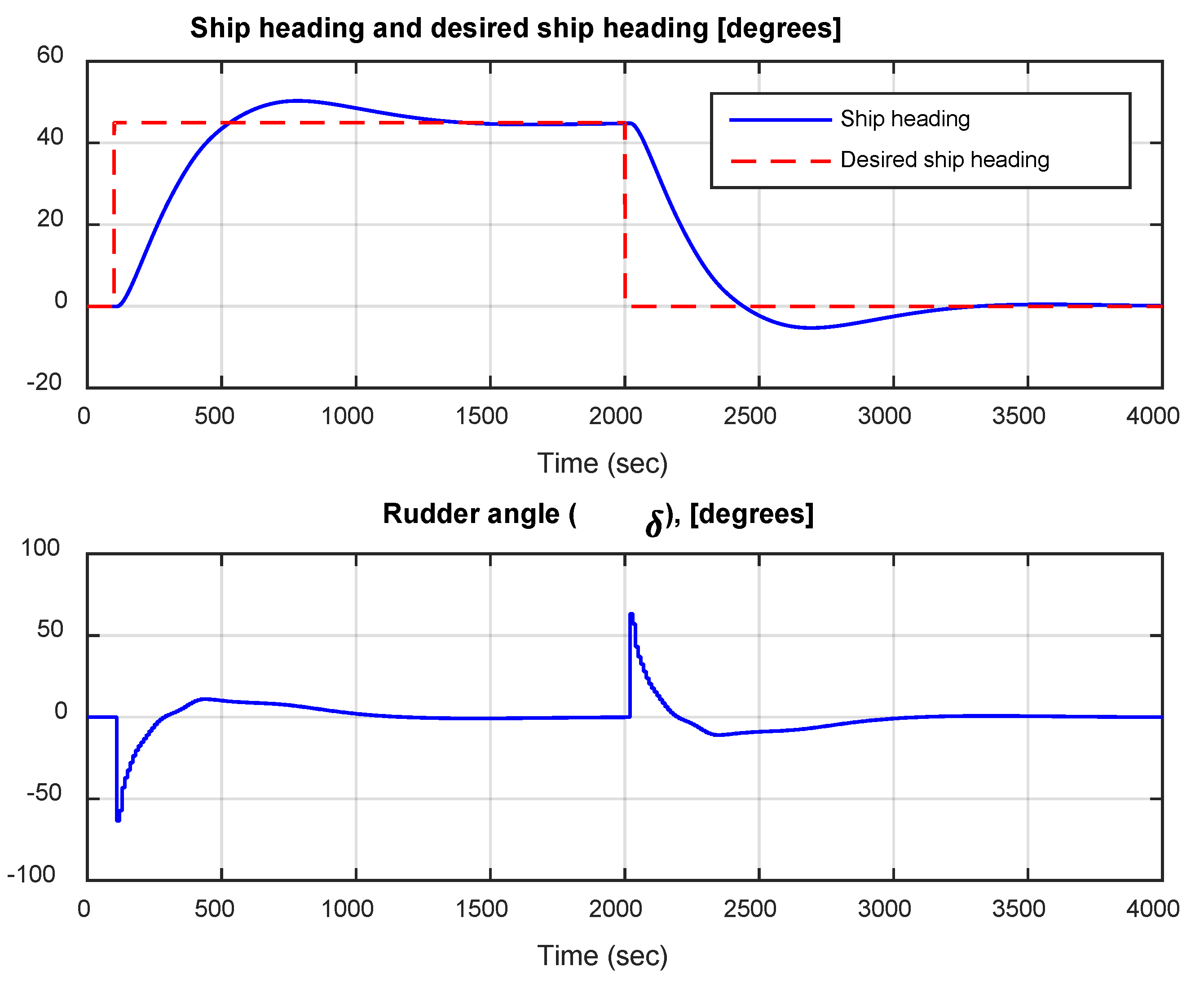
Figure 8.
A closed-loop response of RBFNN for the ship steering at full rather than ballast conditions.
Figure 8.
A closed-loop response of RBFNN for the ship steering at full rather than ballast conditions.
Disclaimer/Publisher’s Note: The statements, opinions and data contained in all publications are solely those of the individual author(s) and contributor(s) and not of MDPI and/or the editor(s). MDPI and/or the editor(s) disclaim responsibility for any injury to people or property resulting from any ideas, methods, instructions or products referred to in the content. |
© 2025 by the authors. Licensee MDPI, Basel, Switzerland. This article is an open access article distributed under the terms and conditions of the Creative Commons Attribution (CC BY) license (https://creativecommons.org/licenses/by/4.0/).
Copyright: This open access article is published under a Creative Commons CC BY 4.0 license, which permit the free download, distribution, and reuse, provided that the author and preprint are cited in any reuse.


