1. Introduction
In the design of sites and roads, side-slopes play a crucial role [
1]. They are not only components that connect the original terrain but also determine the scope of the project's impact on the terrain, as well as the volume of earthwork involved [
2,
3]. In the actual environment, the terrain often exhibits undulations, and the width of the side-slope will change accordingly. Therefore, accurately calculating the intersection of the side-slope with the terrain is a key issue in side-slope modeling. To address this problem, the common method is to perform transverse sampling along the route, then calculate the characteristic points of the side-slope line in the cross-section (including turning points and intersection points with the terrain), and connect the characteristic points of two cross-sections in sequence to build a three-dimensional model of the side-slope. For example, Civil 3D [
4] uses sample lines to obtain terrain cross-sections, then adds the designed road template to the cross-section, and calculates the side-slope toe. By generating side-slope characteristic lines through cross-sections, a corridor is created based on these lines. Similarly, software such as OpenRoads Designer [
5] and HintCAD [
6] also use this method. The advantages of this method are its simplicity in calculation and the ability to add various components in the cross-section using templates, such as ditches. However, this method also has some disadvantages: ① its calculation accuracy is affected by the spacing of the sampling lines; ② the sampling range must be set in advance and cannot be dynamically changed. One way to overcome these shortcomings is to not use cross-sectional sampling but to directly construct a three-dimensional side-slope surface model and calculate the intersection of the side-slope surface with the terrain surface. To our knowledge, there is currently no related research discussing this method. The reason may be that the equation of the side-slope surface is a high-order parametric equation, making it difficult to directly calculate its intersection with the triangular mesh surface.
The goal of this study is to automatically generate a side-slope surface that adapts to the terrain along a given three-dimensional polyline and a terrain surface. This task is divided into three sub-problems: the surface expression of the side-slope, the determination of the excavation and filling types, and the intersection of the side-slope with the original terrain. For the first problem, since the side-slope has the same gradient everywhere, the side-slope surface is a constant gradient surface passing through the given spatial curve. The shape of the spatial curve determines the shape of the side-slope surface, and when the line type of the spatial curve is complex (such as the clothoid used in highway transition curves), the side-slope surface equation becomes complex [
7,
8,
9]. For the second problem, we need to automatically divide the filling section, excavation section, and non-filling and non-excavation section along the spatial curve based on the geometric conditions of the excavation and filling changes, using the given spatial curve and terrain surface. Currently, no research literature has been found on this aspect. Finally, for the third problem, that is, the intersection problem between the surface and the triangular mesh, a large number of literatures have discussed it, and the methods are mainly divided into two categories [
10]: the subdivision method and the marching method. The former [
11,
12,
13] uses the spatial position relationship to find the triangular faces to be intersected from the two surfaces, and the intersection line between the surfaces is formed by connecting the intersection line segments of the triangular faces. The latter [
14,
15,
16] finds the first intersection point and then, starting from this intersection point, uses the topological continuity of the intersection line to track until the entire intersection line is formed.
We propose a two-stage method to solve these problems: the first stage is to automatically determine the excavation and filling types of the side-slope surface along the site boundary line and calculate the equations of each side-slope surface segment; the second stage is to calculate the intersection of each side-slope surface with the terrain triangular mesh. In both stages, an intersection algorithm based on marching tracking is used. In the first stage, we use a line marching algorithm, while in the second stage, we use a surface marching algorithm.
The rest of this paper is organized as follows: First, the side-slope surface equation is derived, and the terrain triangular mesh expression of the half-edge data structure is introduced, see
Section 2. Then, we will propose the two-stage method: in the first stage, the automatic judgment rules for the excavation and filling types of the side-slope surface are derived, and the side-slope surface group equations are determined, see
Section 3. In the second stage, the intersection of the side-slope surface group with the triangular mesh terrain is calculated, see
Section 4. Then, we will create a site model instance using the two-stage method and analyze and compare the performance of this method, see
Section 5. Finally, there is the conclusion section.
2. Geometric Expression
This study involves the representation of two geometric objects. One is the side-slope, which is a plane with a fixed gradient. The other is the terrain surface, which is expressed using triangle meshes.
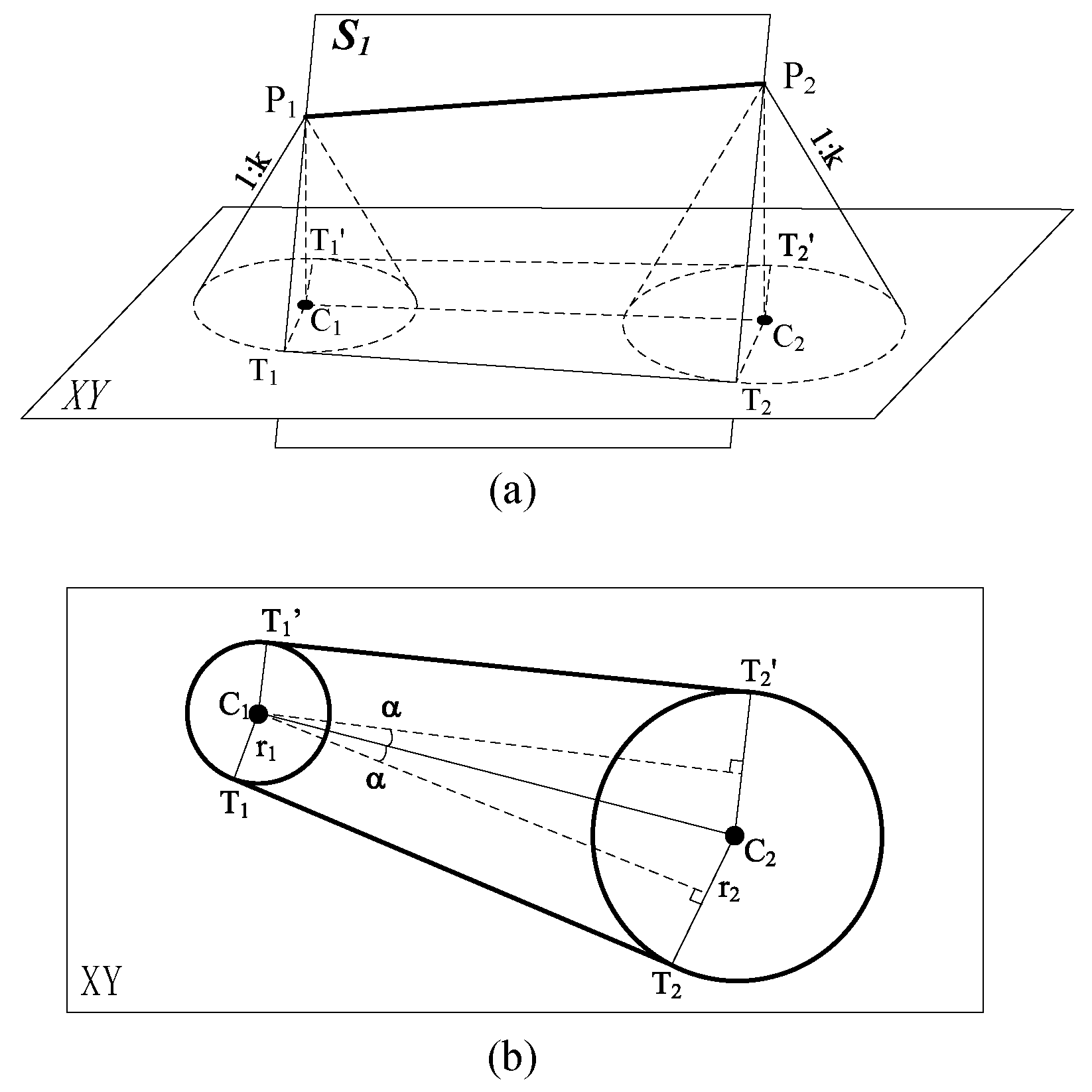
2.1. Side-Slope Plane Equation
The boundary lines P
1P
2...P
n of a known site is a spatial polyline. Consider its first segment P
1P
2, the side-slope plane
S1 passes through this line segment, and the side-slope of the plane is 1:
k, see
Figure 1a. Construct two right cones, their vertices are
P1 and
P2 respectively, and the cone slope is 1:
k. Obviously, plane
S1 is tangent to these two cones, and the intersection points of its tangent line and the XY plane are
T1 and
T2 respectively. To find the plane
S1, let us calculate the point
T1. As shown in
Figure 1b, the circle centers
C1 and
C2 are respectively the projection points of
P1= (x
1, y
1, z
1) and
P2= (x
2, y
2, z
2) on the XY plane. Since the slope of the cone is 1:
k, the radii of the two circles
r1=
k·
z1 and
r2=
k·
z2 are obtained.
let a=x
2−x
1, b=y
2−y
1, c=z
2−z
1, the angle α is given by
Next, the geometric transformation method is used to find
T1 as follow:
C2 rotates 90°+α clockwise around
C1, and then scales r
1/|
C1C2| proportionally, and
T1 is obtained. For these, we apply four transformations to
C2 as
Among them, M1, M2, M3, M4 are four matrices which are responseful for translation, rotation, scaling and translation back respectively:
From (1), (2), the vector
P1T1 is calculated by
Use the same method to get
P1T1'
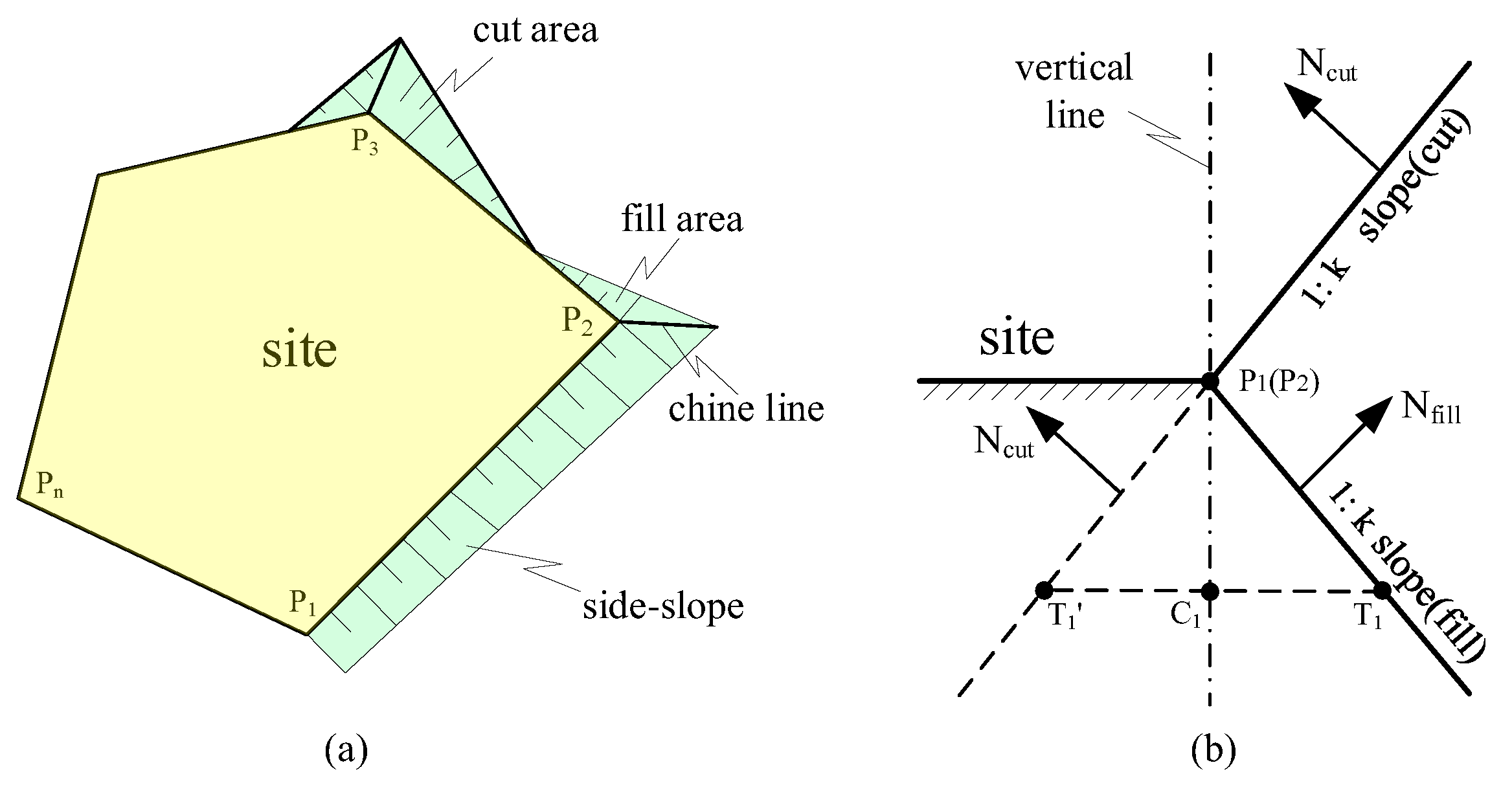
Passing through the line segment
P1P2, there are two planes with a slope of 1:
k to the XY plane. These two planes respectively represent two types of side-slopes in earthworks, shown in
Figure 2. One is an upward slope and the other is a downward slope. The height value of the point on the upward slope is greater than the site height, which is called the slope of cut type; conversely, the downward slope is smaller than the site height, which is the fill type. Because the site boundary lines
P1P2...
Pn are arranged counterclockwise, when moving along the boundary line, the site is always on the left and the slope is always on the right, see
Figure 2. The fill side-slope is determined by three points
T1,
P1, and
P2; while the cut side-slope is determined by three points
T1',
P1, and
P2. Thus, we can calculate the unit normal vectors
Nfill and
Ncut of the fill side-slope
S1 and the cut side-slope
S1' respectively.
Add the fill/cut mark L=±1, and unify the two formulas above as:
When L=1, it signifies Nfill; when L=-1, it denotes Ncut. The value of L can be automatically determined using the method described in section 3.
Thus, given two points
P1(x
1, y
1, z
1),
P2(x
2, y
2, z
2), and the slope value
k, the normal vector
N (
Nx,
Ny,
Nz) of the side-slope plane is obtained. Then, we have the algebraic equation of the side-slope plane:
At the turning points of the site boundary, two side-slope planes intersect to form a chine line. The line can be obtained by these two side-slope planes. Let
N1 and
N2 be the normal vectors of two planes. If the chine line shoots out through the turn point
P, then the directional vector of the chine line is the cross product of the two normal vectors. We have the parametric equation of the chine line
2.2. Terrain Triangle Meshes
2.2.1. Half-Edge Data Structure
Commonly used data structures for representing triangle meshes include [
17]: winged-edge, quad-edge, and half-edge structure. Among them, the half-edge structure splits an edge into two half-edges with opposite directions, which provides excellent topological querying capabilities. In this paper, this data structure is used to represent terrain surface.
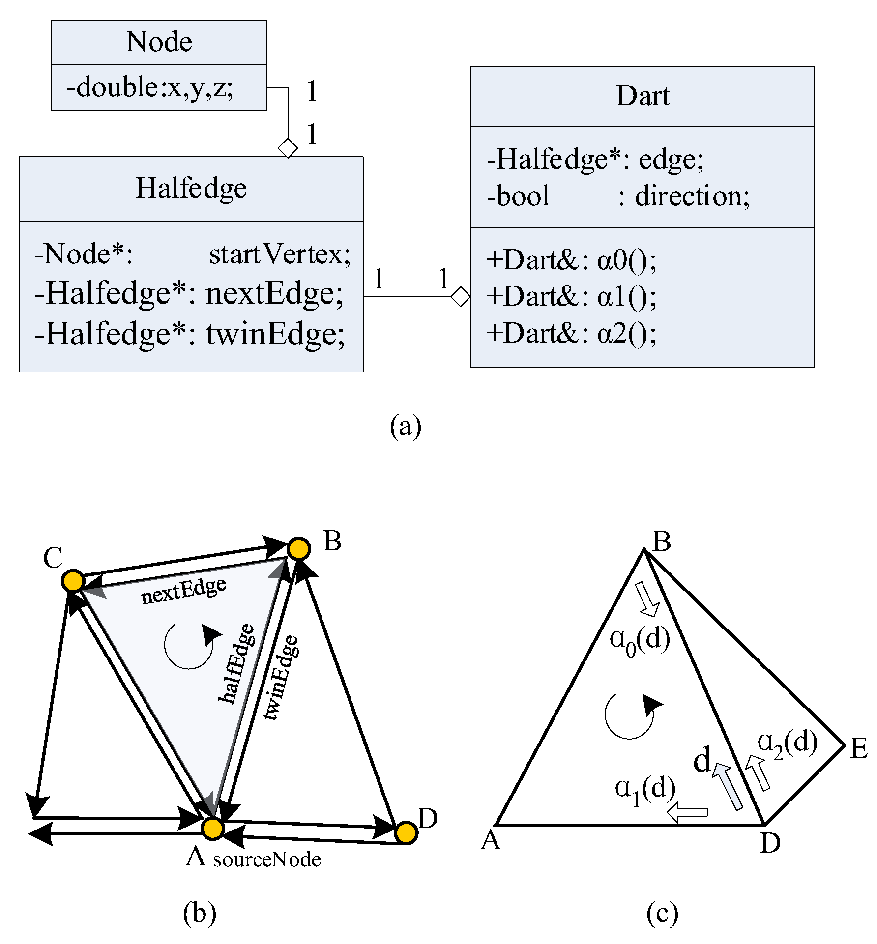
As shown in
Figure 3a, the Half-edge data structure includes a start vertex and two half-edge pointers which point to the nextEdge and the twinEdge accordingly. The former points to the next counterclockwise adjacent edge within the same triangle, the latter points to the opposite edge in the adjacent triangle. A triangle is composed of three half-edges connected counter-clockwise, as illustrated in
Figure 3b. Each half-edge carries geometric and topological information, knowing one half-edge is sufficient to determine the triangle. Taking half-edge
AB as an example in triangle of △
ABC (
Figure 3b), we can access
BC by
AB->nextEdge, and
CA by
AB->nextEdge->nextEdge. Also, we can visit adjacency triangle of △
ADB by
AB->twinEdge. Thereby the topological adjacency relationship in the whole of triangle mesh will be obtained.
In order to make the topological query more convenient, the Dart data structure is used. Dart adds a direction member within the Half-edge to indicate whether the direction of edge is positive or negative.
2.2.2. Topological Combination Operations
Dart can also be regarded as a triplet (
v,
e,
t) composed of vertex, edge, and face [
18]. Using the triplet, we define three basic topological operators
α0(),
α1(), and
α2().
Let d=(
D,
DB,Δ
ADB), shown in
Figure 3c. we have:
These three basic operations can be combined to perform more complex topological operations. The following introduces three α-combination operations that will be used in the intersection algorithm of this paper.
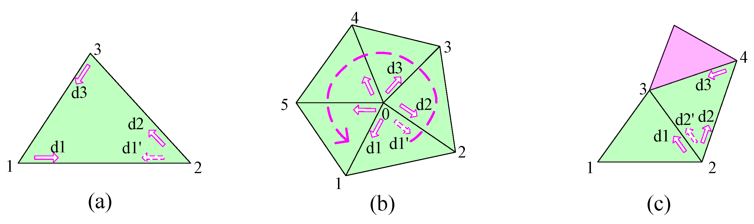
①Edges traversal inside a triangle
As shown in
Figure 4a, given that d1=(1, 12, △123), then d1'=
α0(d1), d2=
α1(d1') =
α1•
α0(d1), d3 =
α1•
α0(d2) =
α1•
α0•
α1•
α0(d1). Here, by repeatedly using the α
1•α
0 operation, one can traverse all the edges of a triangle in a counterclockwise direction.
②Umbrella traversal
Umbrella traversal refers to the sequential visiting all triangles that share a common point. In
Figure 4b, there are five triangles shaped like an umbrella that share point 0 as their common point. Given that d1=(0, 01, △012), then d1'=
α1(d1), d2=α
2(d1')=
α2•
α1(d1), d3=
α2•
α1(d2) =
α2•
α1•
α2•
α1(d1), and so on. So, by repeatedly using the
α2•
α1 operation, one can traverse all triangles sharing a common point in a counterclockwise direction.
③Accessing the edges of adjacent triangle
In
Figure 4c, given d1 in △123, entering into adjacent triangle △324 by d2'=
α2(d1). Next, d2=
α1(d2')=
α1•
α2(d1), d3=
α1•
α0•
α1•
α2 (d1).
3. The First Stage
As seen in
Section 2.1, calculating the side-slope equation requires first determining its type. In this section, by analyzing the changes in fill and excavation types on side-slope surfaces, a rule for inferring changes in fill and excavation types based on intersection points is proposed. Then a method to quickly calculate the intersection point between the boundary line and the terrain surface is given. Through the first stage process, all side-slopes can be established in sections along the boundary lines.
3.1. Rules for Changes in Fill/Cut Side-Slope Types
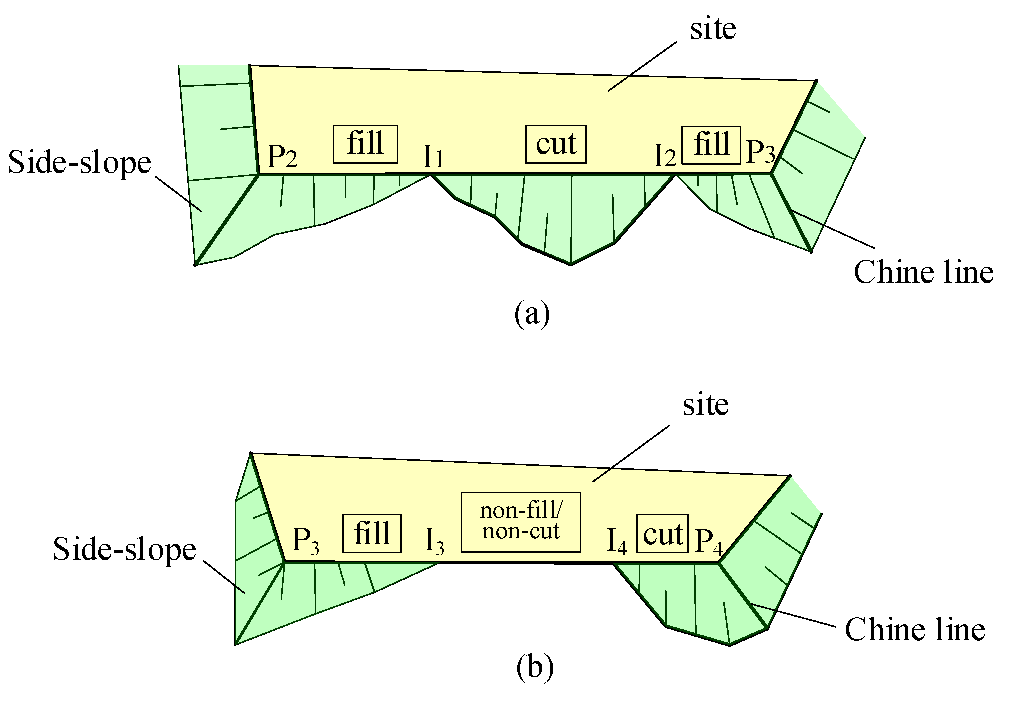
As travelling along the site boundary lines, the boundary will be divided into segments due to the undulations of the terrain. Some segments are above the ground (fill segments) and some are below (cut segments). One method to determine the type of cut and fill is to sample, which is to take a series of sampling points on the boundary line, and compare the height difference between the sampling points and the terrain surface. However, this method is affected by the sampling density. To this end, a new method is proposed that divides fill and cut segments through intersection points and uses continuity to deduce fill or cut types.
By observation, the fill/cut type on the boundary line does not change until the intersection point with the terrain surface is encountered. Therefore, the intersection point is the key to triggering change in fill/cut type. Calculate all intersection points between the boundary line and the terrain surface, and then divide the boundary lines into fill/cut segments. Taking
Figure 5a as an example, on the P
2P
3 boundary line, I
1 and I
2 are the intersection points. To the left of I
1, the side-slope type is fill. As nearing I
1, the side-slope length shortens until it diminishes to zero. After passing I
1, entering the next side-slope, the type of it changes to cut. For point I
2, the fill-cut type is similarly flipped once. To sum up, every time passing through an intersection, the type of side-slope will be reversed, such as fill → cut → fill → cut →...and so on. Another situation needs to be considered here. For the intersection points
I3 and
I4 in
Figure 5b, where the
I3I4 segment are coplanar with the terrain surface, so this section happens to be neither filled nor excavated.
Next, by analyzing the spatial relationship between the boundary line and the terrain triangle, we discuss how the cut and fill type changes. There are three situations of spatial relationships: intersecting, coplanar and disjoint.
①When the boundary line intersects the triangle surface space, part of the triangle is higher than the boundary line and part is lower than the boundary line. The higher part is within the excavation range, and the lower part is within the fill range. Therefore, after such an intersection, the type of side-slope fill/cut will exchange.
②When the boundary line is coplanar with the triangular plane (meaning it has an intersection with both sides), there will be no height difference, no filling and no excavation (that is, non-fill/non-cut section). So, this section will not be generated side-slope.
③If the boundary line and the triangular surface do not intersect or are coplanar, it will not affect the fill and cut type of the side-slope.
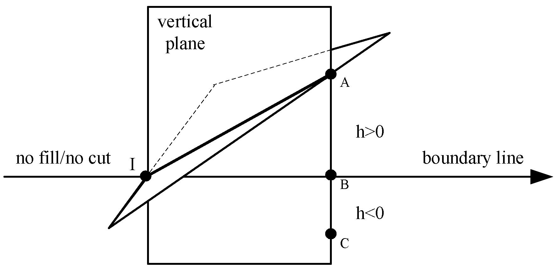
Through the above analysis, all situations and changing conditions of excavation and filling changes are listed, see
Table 1. In the third and second situations in the table, the excavation and fill types change irregularly and require further judgment. To this end, we can calculate the intersection line between the vertical plane where the boundary line is located and the triangular plane where the intersection point is located, as shown in
Figure 6. Point B is the intersection point when the boundary line and the triangular plane are coplanar, and points A and C are above and below point B respectively. Corresponding to these three situations, it is determined that the three types of the new interval are fill or non-fill/non-cut or cut.
To sum up, the necessary condition for judging the change of side-slope fill/cut type along the boundary line is that the boundary line has an intersection with the terrain mesh, but the intersection does not necessarily lead to a change in the side-slope type. The judgment rules are:
Rule 1:
When the intersection is an internal intersection (corresponding to the first case in Table 1), it inevitably leads to a change in side-slope type, at which intersection point the excavation and filling types reverse: if the last section is filling, this section must be excavation, and vice versa. when the intersection point is the intersection point on the edge of the triangle (corresponding to the 2nd and 3rd situations in Table 1), it does not necessarily lead to a change in the side-slope type. In this case, the first boundary line passing through the intersection point needs to be taken. A triangular surface is used to determine the side-slope excavation and fill type of the next boundary line. Finally, if there is no intersection (corresponding to the fourth situation in Table 1), the side-slope cut/fill type will not change.
3.2. Finding the Intersecting Triangles in Mesh
From the above analysis, finding the intersection point between the boundary line and the terrain mesh is the key to determining the fill/cut type of side-slope. Using the topological of the half-edge structure, the number of intersecting triangle patches to be solved can be greatly reduced. The basic idea is: first in 2D space, all the triangles to be intersected with the boundary line are found using the topology query of the half-edge structure. Then in three-dimensional space, find the exact intersection points of the boundary line and the space triangle.
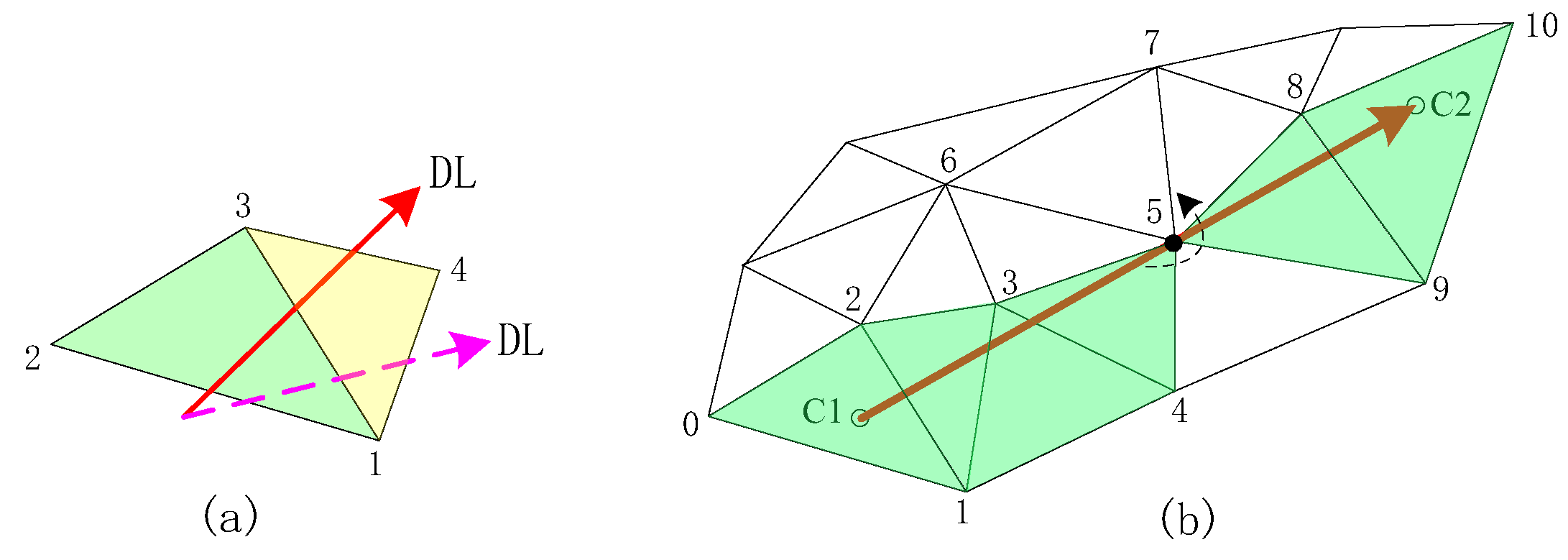
Examine the topological relationship between the intersection of the directed line and the triangle on the plane: as shown in
Figure 7a. If the directed line DL intersects an edge 13 of △132, then the next intersecting triangle is the adjacent triangle △143, which shares the common edge 13. When entering in △143, the next intersecting edge can only be the edge 14 or the edge 43. In order to determine which edge it is, we just determine whether the vertex 4 is on the left of the directed line or not. If so, the next intersecting edge is the edge 14, otherwise the edge 43.
Figure 7b is the complete process of traversing the triangular mesh to be intersected, where the triangles found are △012 → △132 → △143 →△453 → △598 → △9108.
While traversing along the specified path, it is crucial to swiftly identify the triangles within which points C1 and C2 are situated. Additionally, we must ascertain whether the vertices of these triangles lie to the left of the directed line. We adopt the
locateTriangle algorithm and
Left predicate by O'Rourke [
19].
3.3. Calculation of Intersection Points Between Boundary Lines and Terrain Mesh
Once obtained all intersecting triangles with the directed line in the two-dimensional space. We compute the spatial intersection point between the three-dimensional boundary line and the plane which determined by each triangle. Let the equation of this plane be:
n•
P+
D=0. The two endpoints of the boundary line segment are
P1 and
P2, and its straight-line parameter equation is:
P(
t)=
P1+
t·(
P2-
P1). If
n•(
P2-
P1) ≠ 0, the boundary line intersects the plane where the triangular surface is located. Bringing the boundary line parameter equation into the plane equation, we get
t=(n•
P1+
D)/n•(
P1-
P2). So the intersection point of the straight line and the plane is:
Next, we use locateTriangle algorithm to examine whether the point I is in the triangle. Only those points that satisfy the location conditions are the exact intersection points.
3.4. Determine the Side-Slope Type and Its Equation Piece by Piece
For the entire boundary line, the algorithm along the line calculates the intersection points, and then sorts the intersection points and boundary line turning points in counterclockwise order to form an ordered point set. Take two points from the point set to calculate the side-slope equation of each section. Specific steps are as follows:
|
Algorithm1. Traveling-along-line |
Input: Terrain mesh M, boundary lines PL , Slope value kfill and kcut;
Output: Side-slope equations for each segment on the boundary line, Eqs{}
ordered point set (intersection point + turning point);
1. fetch the first turning points P1of PL;
2. △t:=LocateTriangle(P1,M)
3. IF above(P1, △t) THEN L:= 1
4. ELSE L:= -1
5. IF (L==1) THEN k:= kfill
6. ELSE k:=kcut
7. FOREACH (P1,P2) IN PL segments
8. Ints:=intersect(P1P2,M)
9. P:=P1
10. FOREACH I IN Ints
11. Eq:=side-slopeEq(P, I, L, k)
12. Eq:=null if L==0
13. L:=-1*L
14. P:=I
15. Eqs←side-slopeEq(P, P2, L, k) |
4. The Second Stage
In this section, we use continuity to quickly calculate the intersection between each side-slope plane and the terrain mesh.
4.1. Topological Continuity of the Intersection Between the Side-Slope Plane and the Triangular Mesh
4.1.1. Spatial Relationship Between Plane and Triangle
There are three positional relationships between a point in space and the plane: located to the left, right and above the plane, then there will be 3
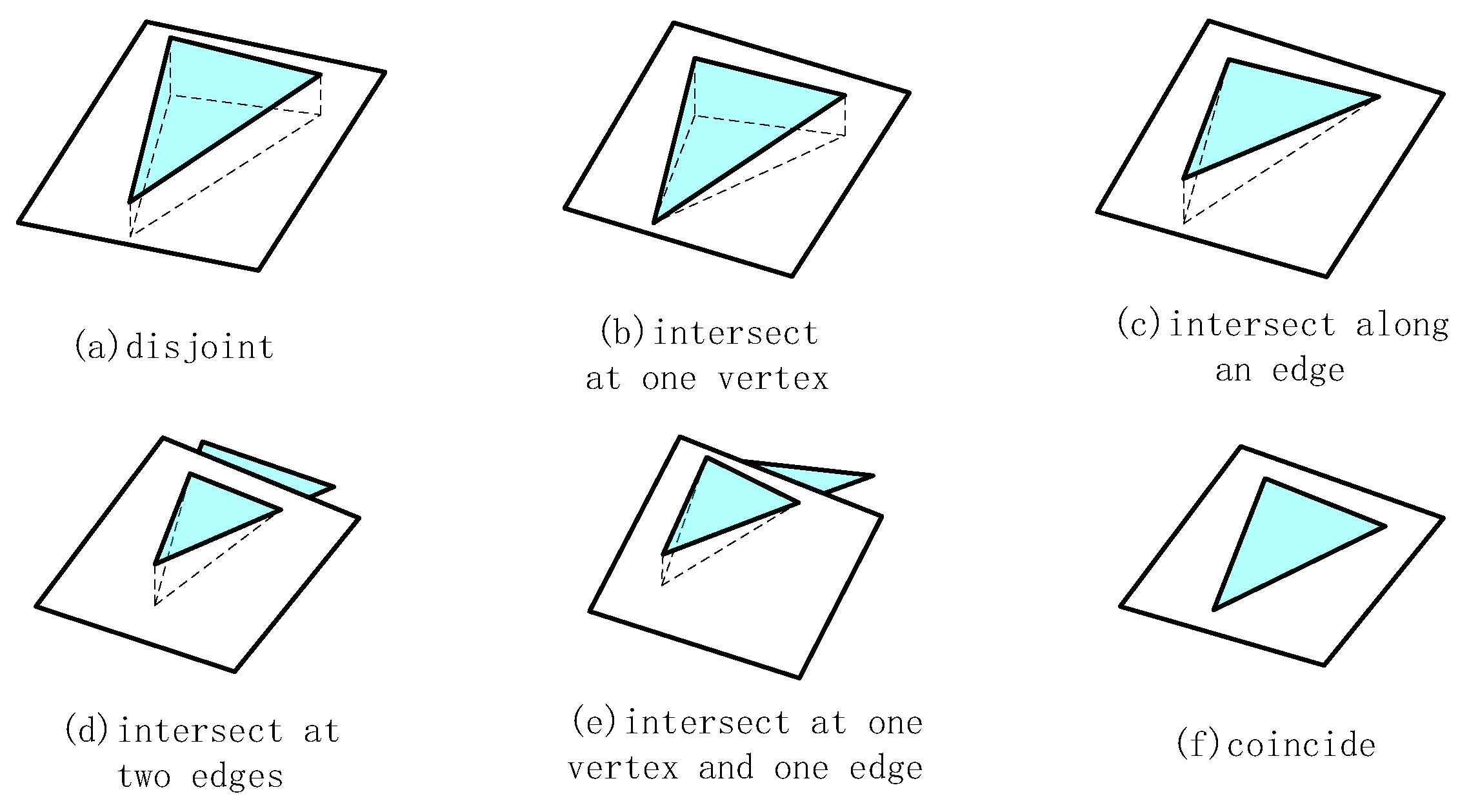
3 = 27 combinations of relationships between the three vertices of the triangle. Considering symmetry, the 27 relationships can be combined into the following 6 types: ① Three vertices are on one side of the plane (do not intersect); ② One vertex is on the plane and the other two vertices are on one side of the plane (intersect at one point); ③ Two vertices On the plane (intersects on one side); ④ One vertex is on one side of the plane and the other two vertices are on the other side of the plane (intersects on both sides) ⑤ One vertex is on the plane and the other two vertices are on different sides of the plane (intersects on one point and one side) ); ⑥ The three vertices are all on the plane (coincident), see
Figure 8.
4.1.2. Topological Continuity Analysis
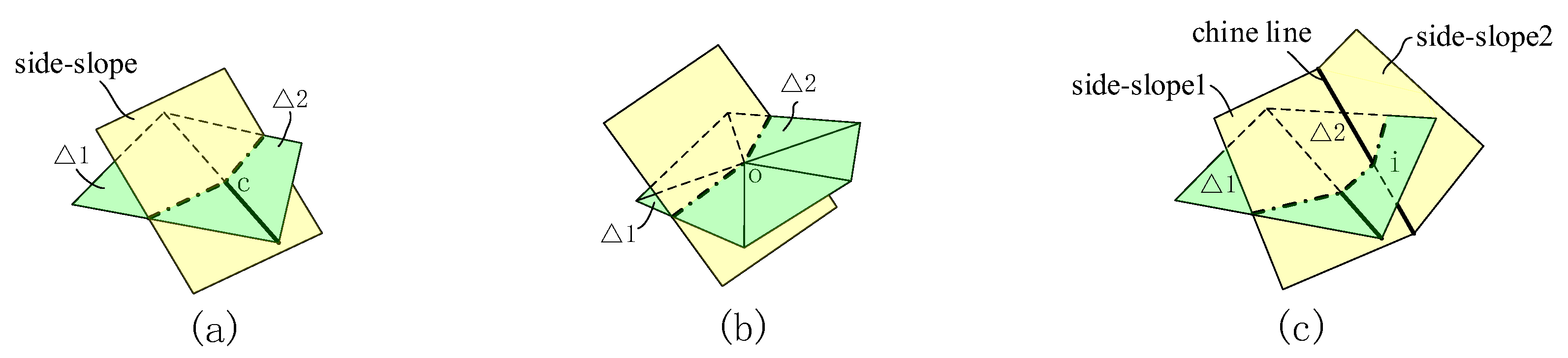
The triangular mesh is composed of continuous triangles, so the intersection between the side-slope and the triangular mesh is also continuous. According to the spatial relationship between a plane and a triangle, if a plane intersects the first side of a triangle, then the next intersection can only be the vertex or another side of the triangle. In this way, the intersection between the side-slope surface and the triangular mesh has three continuous situations: ①
Figure 9a, when the side-slope surface intersects △1, it also intersects △2 which is adjacent to △1. The side-slope connects with the intersection segments of the two triangles at point
c on the common edge. ②
Figure 9b, if the side-slope intersects at the vertex
o of △1, then the next triangle that intersects the side-slope is a triangle with
o as the common point. The side-slope connects with the intersection segment of the two triangles at the common point
o. ③
Figure 9c, two intersecting side-slopes intersect with the same △2, then △2 has two intersection segments with each of the two side-slopes, and the two segments meet at the intersection
i of the chine line and △2.
4.2. Algorithm of Traveling Along Plane
Determining which side of the plane a point is on is called lateral judgment of the point plane. It is known that the plane equation is Ax+By+Cz+D=0, let the function e(x,y,z)= Ax+By+Cz+D. For any point P(x,y,z), if e(P)>0, then P is on one side of the normal vector direction of the plane; if e(P)<0, on the other side; such as e(P) =0, then P is on the plane. Obviously, for a line segment, if its two endpoints are on different sides of the plane, the line segment intersects the plane.
Similar to the traveling along line algorithm (Algorithm1.), the traveling along plane algorithm also uses the properties of the half-edge structure to quickly traverse the triangles to be intersected. The main difference is that the intersection line is not on a straight line but on a plane, and the point-surface lateral judgment is used to determine whether the edge intersects the surface.
4.3. Calculate the Intersection Line Between the Side-Slope Surface and the Terrain Mesh
The method of finding the intersection between a side-slope group and a triangular mesh is to find the intersection lines with the triangular mesh for each side-slope in the group one by one. During the intersection process, the first triangle that intersects with the side-slope group is found, and then the triangles to be intersected are found one by one using the surface traveling algorithm. When the intersection line encounters an edge, it goes to the next side-slope, and the side-slope group is processed in this loop until the last side-slope. Specific steps:
|
Algorithm 2. Traveling-along-planes |
Input: Boundary lines PL; Equations of side-slope planes {Eqs}; Terrain mesh M
Output: The intersection lines {INTs} between side-slope planes and terrain mesh
1. Find the first triangle that intersects the side-slope.
2. R(t)=P1+(N2×N1)•t //Equation (5)
3. i:=intersect(R(t), M)
4. △t:=LocateTriangle(i,M)
5. FOREACH side-slope plane sp IN Eqs:
6. △t2:=LocateTriangle(P2, M)
7. WHILE △t≠△t2 DO:
8. INTs←INTs+intersect(sp, △t)
9. △t:=AdjcentAngle(eq, △t) |
5. Discussion
On the Visual Studio 2019 platform, the C++ development language and the OpenGL graphics library and the open source library TTL (Triangulation Template Library) provided by Hjelle [
20] were used to implement the algorithm proposed above. Hardware environment: CPU Intel i5, memory 2.0GB.
5.1. Example
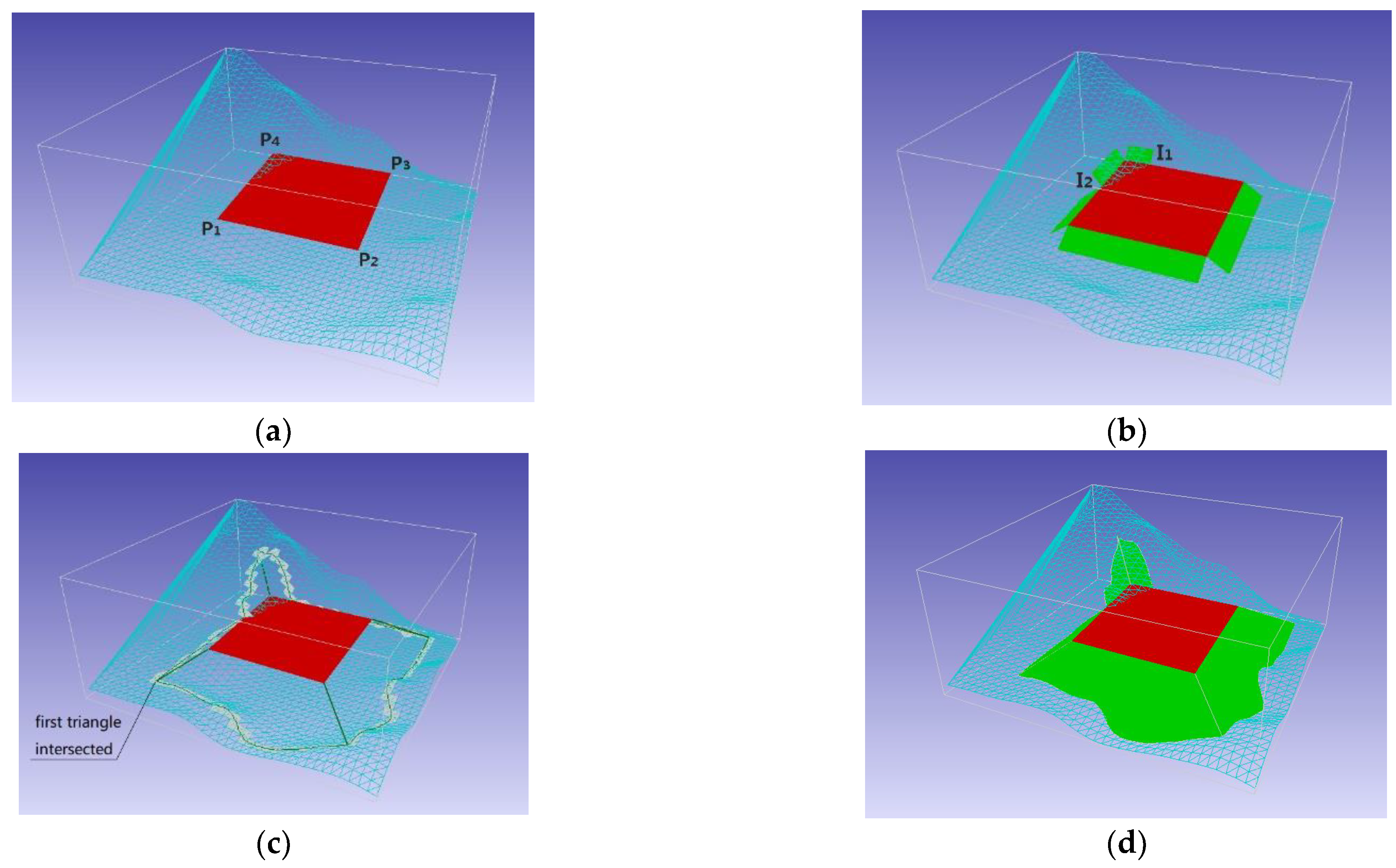
As shown in
Figure 9a, there are a total of 1482 vertices and 2848 triangles in the original terrain triangulation mesh. The design site is a rectangular area with four turning points: P
1(8709.00, 7992.00, 15.00), P
2(8712.00, 8050.00, 15.00), P
3(8695.00, 8045.00, 15.00), P
4(8690.00, 7980.00, 15.00), and the cut and fill grade adopted are 1:0.75 and 1:1.5 respectively. The site turning point P
4 is lower than the terrain surface, and the other three turning points are higher than the terrain, so it is a half-filled and half-excavated site.
Figure 9b shows the first stage of our method, as
Algorithm 1. Traveling along the boundary polyline P
1P
2P
3P
4, two spatial intersection points I
1 and I
2 between the boundary line and the terrain surface are calculated, so that the entire boundary line is divided into six segments. First, we determine the point P
1 is above the terrain mesh, so it is in the fill section. Then we deduce the fill/cut types of subsequent sections by the
Rule 1.
Table 2 provides a detailed process for deducing the fill/cut type of six sections. Finally, the fill/cut types for each side-slope are identified, totaling four filling and two excavating ones.
Using the results from
Table 2, we can then establish the equation of each side-slope plane. Taking the first row of
Table 2 as an example, we show how to compute it. From the first row, we get parameters of the first side-slope plane, as follows:
Then, substitute the above parameters into equation (3), we obtain the normal of the first side-slope plane:
and the plane equation:
In the same way, we can obtain all side-slope planes, which are temporarily drawn according to the unit slope length in
Figure 9b.
The second stage of our method is shown in
Figure 9c, in the process of calculating the intersection along the side- slope plane by the
Algorithm 2. First, we should find the first triangle intersected by computing the first chine line hitting the mesh. Using Equation (5), we have the equation of the chine line:
•t
After identifying the first intersecting triangle, the marching algorithm is then used to determine all intersecting triangles sequentially. In
Figure 9c, the gray triangles in the mesh are those to be intersected found.
Figure 9c also shows four chine lines at the corners and the final intersection lines between the side-slope plane and the triangular mesh.
Figure 9d shows the final result after rendering the side-slope surfaces.
Figure 10 is an example of modeling a terrace site and a road embankment using our method in the paper. The boundary lines of the embankment in the figure should be curve at the turning point. In order to use our method, multi-segment polylines are applied to approximate the curve and generate the subgrade side-slope model.
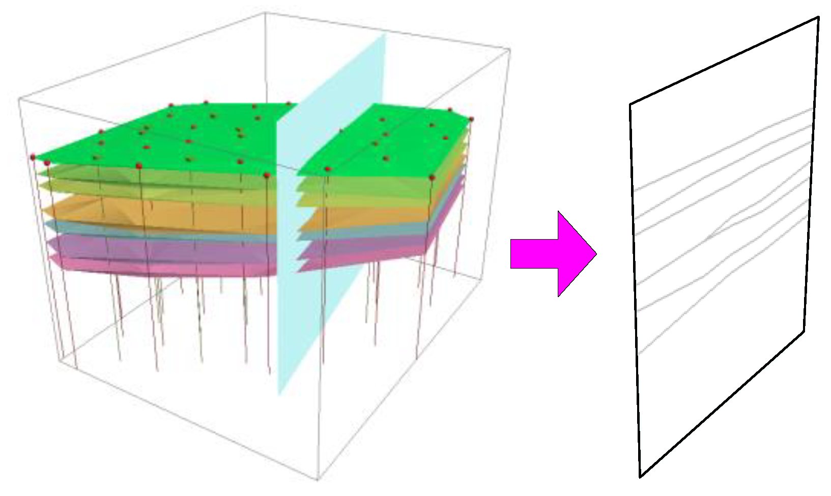
The surface traveling algorithm in this article can also be used to calculate stratigraphic profiles. At this time, the side-slope surface becomes a section plane, and each layer is still a triangular mesh surface. The stratigraphic profiles are obtained by calculating the intersection lines between the section plane and the stratigraphic triangular mesh, see
Figure 12.
5.2. Analysis
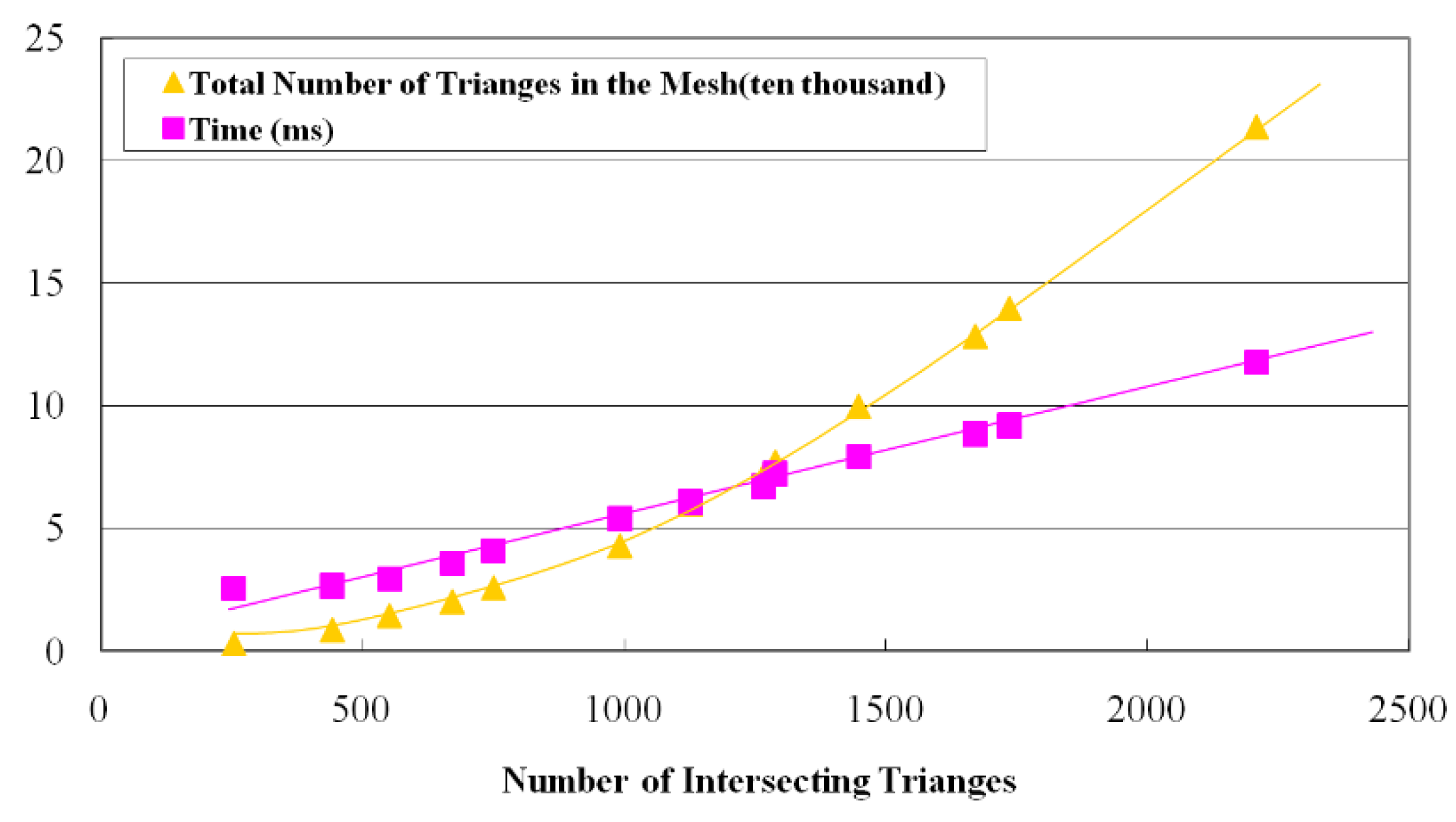
The main access operations of our two-stage method proposed in this article are point positioning and lines/surfaces traversal. The average time complexity of the algorithm for point positioning operations is O (logN) (N is the number of triangles in the mesh). For the traversal algorithm along a line/surface, it visits only a strip of the triangulation mesh, not the entire triangles within the mesh. In order to estimate the relationship between algorithm efficiency and the number of triangles in the mesh, the terrain triangular mesh depicted in
Figure 10 is subdivided.
Table 3 shows the changes in the number of intersecting triangles during traversal and the total calculation time as the total number of triangles in the mesh increases. It can be observed from
Figure 13 that the total number of triangles in the mesh and the number of intersecting triangles exhibit a roughly parabolic trend, while the number of intersecting triangles and the calculation time show a roughly linear relationship.
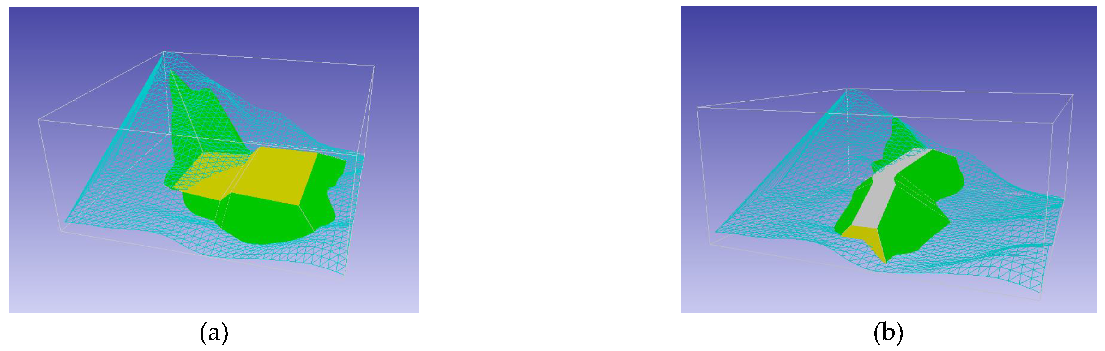
5.3. Comparison
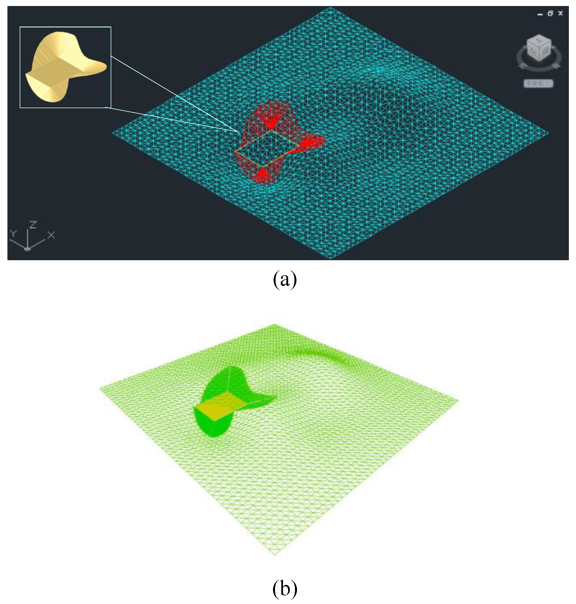
The commercial software Civil3D 2016 was used to compare with our method in this section. The model is shown in
Figure 14. In the figure (a) is the three-dimensional wireframe diagram of the site and side-slope generated with Civil3D (the upper left corner is the rendering), (b) is the three-dimensional diagram generated by the method in this section. Comparing the two figures, we can see that there is basically no difference between the two models in terms of fill and excavation segments, side-slope shape, etc. After testing, the total time for generating the side-slope model by our method is 2.2ms, while the time used by Civil3D is >200ms, so the time efficiency improvement of this method is considerable. In addition, the algorithm in this paper is also compared with the intersection algorithm based on subdivision [
21]. The comparison of algorithm time is shown in
Table 4.
6. Conclusion
The intersection lines between the side-slope and the terrain surfaces provides a more efficient and accurate approach for determining the cut/fill type of a side-slope compared to discretizing the entire surface with numerous points. It reduces computational costs while maintaining the necessary level of precision for analyzing the interaction between the side-slope and the terrain.
The two-stage method proposed in this article is based on the traveling algorithm on the triangle mesh. Due to the use of the continuity of the intersection line and the operation based on the half-edge structure, the number of intersection triangles to be calculated is greatly reduced, and the method is fast in calculation and efficient. The intersection points have been arranged in order during the travel process, and there is no need to re-sort the intersection points. The accuracy of the generated intersection lines is related to the accuracy of the terrain triangulation mesh. Given the original terrain and site boundaries, the two-stage method can automatically find all side-slopes, determine side-slope types and calculate intersections, without the need for interactive operations.
The algorithm presented in this article is founded on the side-slope boundary with polylines. However, this approach falls short when it comes to precisely depicting side-slopes with curved boundaries, due to the necessity for a novel surface equation. For surfaces with curved side-slopes, the fundamental concept of the two-stage algorithm introduced here remains viable. Nevertheless, adjustments are required for the point-line lateral direction determination algorithm employed in the traveling-along-line algorithm: the cross-multiplication method is inadequate for ascertaining the lateral direction of points relative to curves, necessitating the development of an alternative approach. Additionally, in the traveling-along-planes algorithm, while the curve side-slope can be articulated as algebraic equations and point-surface lateral judgment algorithms remain effective, a new technique is essential for calculating the intersection between a triangle edge and a surface. Addressing these enhancements is slated for future work.
Funding
Please add: This research was funded by the "Research Funds of Sichuan Province Engineering Technology Research Center of BIM+ Application and Intelligent Visualization" (Grant No. BIM-2024-Y-01), and the "Panzhihua City Guided Science and Technology Plan Project" (Grant No. 2024ZD-G-13)
Data Availability Statement
Data are contained within the article.
Conflicts of Interest
The author declare no conflict of interest.
References
- Glaeser, G. Geometry and its Applications in Arts, Nature and Technology[M]; Springer International Publishing, 2020; pp. 201–206. [Google Scholar]
- Hare, W.; Lucet, Y.; Rahman, F. A mixed-integer linear programming model to optimize the vertical alignment considering blocks and side-slopes in road construction. European Journal of Operational Research 2015, 241, 631–641. [Google Scholar] [CrossRef]
- Momo, N.S.; Hare, W.; Lucet, Y. Modeling side slopes in vertical alignment resource road construction using convex optimization. Computer-Aided Civil and Infrastructure Engineering 2023, 38, 211–224. [Google Scholar] [CrossRef]
- Yuan, L.; Liu, S.; Meng, L. Numerical simulation analysis of slope stability from rainwater utilizing the Civil3D+Flac3D coupling. Desalination and Water Treatment 2024, 319, 100517–100527. [Google Scholar] [CrossRef]
- OpenRoads Designer, Roadway Design Software. Available online: https://www.bentley.com/software/openroads-designer/ (accessed on 12 September 2024).
- HintCAD(in Chinese). Available online: https://www.hintcad.cn/product/3862.html (accessed on 15 October 2024).
- Hartmann Erich. Geometry and algorithms for computer aided design[M]. Darmstadt University of Technology 95 (2003).
- Kozniewski, E.; Kozniewski, M.; Orlowski, M.; et al. Modeling an embankment with a natural slope. Journal Biuletyn of Polish Society for Geometry and Engineering Graphics 2013, 25, 49–56. [Google Scholar]
- Zhou, F.; Li, C.; Ding, Y. Developable iso⁃slope surface and its application to slope modeling[J]. Journal of Wuhan University(Engineering Edition) 2019, 52, 610–615. [Google Scholar]
- Yang, P.; Qian, X. Direct boolean intersection between acquired and designed geometry[J]. COMPUTER AIDED DESIGN 2009, 41, 81–94. [Google Scholar] [CrossRef]
- Lin, H.; Qin, Y.; Liao, H.; et. al. Affine arithmetic based B-Spline surface intersection with GPU acceleration[J]. IEEE transactions on visualization and computer graphics 2013, 20, 172–181. [Google Scholar]
- Shou, H.-H.; Zhou, C. Triangular grid intersection based on hierarchical enclosing box and average cell[J]. Journal of Zhejiang University of Technology 2018, 46, 540–543. [Google Scholar]
- Shi, Y.; Zhang, Y.; Cheng, T.; et al. Intersection algorithm for surface segmentation based on space polygon triangulation[J]. Journal of Graphics 2019, 40, 447–451. [Google Scholar]
- Elsheikh, M. A reliable triangular mesh intersection algorithm and its application in geological modelling[J]. Engineering with Computers 2014, 30, 143–157. [Google Scholar] [CrossRef]
- Svelander, F.; Kettil, G.; Johnson, T.; et al. Robust intersection of structured hexahedral meshes and degenerate triangle meshes with volume fraction applications[J]. Numerical Algorithms 2018, 77, 1029–1068. [Google Scholar] [CrossRef]
- Ventura, M.; Soares, G. Surface intersection in geometric modeling of ship hulls[J]. Journal of Marine Science and Technology 2012, 17, 114–124. [Google Scholar] [CrossRef]
- Botsch, M.; Pauly, M.; Kobbelt, L.P.; et al. Geometric Modeling Based on Polygonal Meshes[M]. Eurographics 2008 Tutorial Notes, Crete, Greece, 2008:17-18.
- Bradley, P.; Paul, N. Comparing G-maps with other topological data structures. geoInformatica. 2014, 18, 595–620. [Google Scholar] [CrossRef]
- O'Rourke, J. Computational geometry in C[M]; China Machine Press: Beijing, 2005; pp. 239–245. [Google Scholar]
- Hjelle, Ø.; Dæhlen, M. Triangulations and applications[M]; Springer Science & Business Media, 2006; pp. 25–28. [Google Scholar]
- Zhao, J.; Bai, R.; Liu, G.; et al. Research on TIN fast intersection algorithm and its application[J]. Computer Application Research 2016, 33, 3667–3670. [Google Scholar]
Figure 1.
Construction of side-slope plane (a) Axonometric view (b) Top view.
Figure 1.
Construction of side-slope plane (a) Axonometric view (b) Top view.
Figure 2.
Fill/cut type of side-slope (a)Plan View (b) Section View.
Figure 2.
Fill/cut type of side-slope (a)Plan View (b) Section View.
Figure 3.
Halfedge data structure (a)class diagram (b)half-edge (c)three topological operators.
Figure 3.
Halfedge data structure (a)class diagram (b)half-edge (c)three topological operators.
Figure 4.
Three compostions α operations (a)iterate three edges of a triangle (b)umbrella traversal (c)visit adjacent triangle.
Figure 4.
Three compostions α operations (a)iterate three edges of a triangle (b)umbrella traversal (c)visit adjacent triangle.
Figure 5.
Changing on type of side-slope (a)alternating fill or cut segments (b)non-fill/non-cut segments exist.
Figure 5.
Changing on type of side-slope (a)alternating fill or cut segments (b)non-fill/non-cut segments exist.
Figure 6.
Fill/cut type judgment when the intersection is on the edge of triangle.
Figure 6.
Fill/cut type judgment when the intersection is on the edge of triangle.
Figure 7.
Algorithm of marching along direction line (a) The topological relationship of directed line intersecting triangle (b) The process of traversing the triangular mesh.
Figure 7.
Algorithm of marching along direction line (a) The topological relationship of directed line intersecting triangle (b) The process of traversing the triangular mesh.
Figure 8.
Space relation between plane and triangle.
Figure 8.
Space relation between plane and triangle.
Figure 9.
Continuity of intersection line between side-slope and trimesh (a)Common edge (b)Common vertex (c)Common chine line.
Figure 9.
Continuity of intersection line between side-slope and trimesh (a)Common edge (b)Common vertex (c)Common chine line.
Figure 10.
The process of building side-slope (a)Starting situation (b)The first stage (c)The second stage (d) Final result.
Figure 10.
The process of building side-slope (a)Starting situation (b)The first stage (c)The second stage (d) Final result.
Figure 11.
Modeling cases (a) terrace site (b)road embankment.
Figure 11.
Modeling cases (a) terrace site (b)road embankment.
Figure 12.
Stratum profiles.
Figure 12.
Stratum profiles.
Figure 13.
Relation between number of intersected triangles and total number of triangles in mesh and calculation time.
Figure 13.
Relation between number of intersected triangles and total number of triangles in mesh and calculation time.
Figure 14.
Comparison of modeling result (a) Civil3D 2016 (b) Our method.
Figure 14.
Comparison of modeling result (a) Civil3D 2016 (b) Our method.
Table 1.
Rules of conversion on fill/cut type of side-slope.
Table 1.
Rules of conversion on fill/cut type of side-slope.
| No. |
Spatial Relationship between Boundary Line and Triangle Surface |
Change in Fill/Cut Type |
| 1 |
Intersecting && Intersection Point Inside the Triangle |
Reversal at the intersection point, either from fill to excavation or from excavation to fill |
| 2 |
Intersecting && Intersection Point on One Side of the Triangle |
No change in fill/cut type |
| 3 |
Coplanar (two intersection points on the triangle edge) |
This segment becomes neither fill nor excavation; the type of the next segment is determined by the method in Figure 6
|
| 4 |
Not Intersecting |
No change in fill/cut type |
Table 2.
Segmented Calculation of Side-Slope Plane.
Table 2.
Segmented Calculation of Side-Slope Plane.
| No. |
Start point |
point type |
end point |
inverse |
fill/cut type |
L sign |
Slope value |
| 1 |
P1
|
Turning Point |
P2
|
false |
fill |
1 |
1:1.5 |
| 2 |
P2
|
Turning Point |
P3
|
false |
fill |
1 |
1:1.5 |
| 3 |
P3
|
Turning Point |
I1
|
false |
fill |
1 |
1:1.5 |
| 4 |
I1
|
Intersection Point |
P4
|
true |
cut |
-1 |
1:0.75 |
| 5 |
P4
|
Turning Point |
I2
|
false |
cut |
-1 |
1:0.75 |
| 6 |
I2
|
Intersection Point |
P1
|
true |
fill |
1 |
1:0.75 |
Table 3.
Calculating time with numbers of triangle.
Table 3.
Calculating time with numbers of triangle.
| Total Number of Triangles in the Mesh |
Number of Intersecting Triangles |
Time (ms) |
| 2848 |
254 |
2.5682 |
| 8544 |
442 |
2.6644 |
| 14240 |
551 |
2.9308 |
| 19936 |
671 |
3.5895 |
| 25632 |
750 |
4.1023 |
| 42720 |
991 |
5.4027 |
| 59808 |
1126 |
6.0809 |
| 71200 |
1265 |
6.7120 |
| 76892 |
1288 |
7.2347 |
| 99680 |
1447 |
7.9305 |
| 128160 |
1670 |
8.8576 |
| 139552 |
1735 |
9.1974 |
| 213600 |
2207 |
11.7620 |
Table 4.
Calculating time comparison with intersection algorithm based on subdivision.
Table 4.
Calculating time comparison with intersection algorithm based on subdivision.
| Total Number of Triangles in the Mesh |
ZHAO [21] (ms) |
Our method(ms) |
| ~19000 |
229 |
3.59 |
| ~139000 |
2604 |
9.20 |
| ~250000 |
5104 |
13.21 |
|
Disclaimer/Publisher’s Note: The statements, opinions and data contained in all publications are solely those of the individual author(s) and contributor(s) and not of MDPI and/or the editor(s). MDPI and/or the editor(s) disclaim responsibility for any injury to people or property resulting from any ideas, methods, instructions or products referred to in the content. |
© 2024 by the authors. Licensee MDPI, Basel, Switzerland. This article is an open access article distributed under the terms and conditions of the Creative Commons Attribution (CC BY) license (http://creativecommons.org/licenses/by/4.0/).