A Probabilistic Expanding Universe

1. Introduction

Our understanding of theories beyond the standard paradigm was driven by our efforts of unifying further the several forces and theories describing the basic elements of our universe which have been discovered and developed over the years. This led to an unresolved issue, which is a basic way to unify all those forces and theories, namely the grand unification theory (GUT). To resolve this issue, our best approach was to combine two rather successful theories, which describe most of our observations. Gravity is our best understanding of the world at infinitely large. Gravity theory has been informed by general relativity (GR) theory which taught us several aspects beyond our naive understanding of the concepts describing nature from the very large to the very small scales and the very low to the very high energetic aspects of our universe. In parallel, quantum field theory (QFT) is a successful physical theory with our best description of the quantum, infinitesimal small world. This theory introduced the concept of probabilities as a part of nature and the universe, in the sense that particles behave also as probabilistic waves or fields. Quantum gravity, a long-standing point in theoretical physics, is the first idea of merging the QFT and the gravity, in a unified mathematical frame study, are several outstanding efforts which approach resolutions for this issue, with the most popular ones considering the string theory perspective [1,2,3,4,5], to the loop quantum gravity perspective [6]. Extraordinarily, there is a fine relationship between QFT and gravity in the large N-limit of superconformal field theory and supergravity, namely the Anti-de Sitter conformal field theory correspondence, or AdS/CFT correspondence [7], right after the revision of Anti-de Sitter space and holography [8]. This mathematical constructs for physical systems indicate a very fruitful point in spacetime. Note that fruitful ideas sometimes rise when we entertain them in a light and playful discussion. Such ideas extend the cosmological paradigm when we even consider coupled quintessence fields [9] fields behaving in a `rollercoaster” frame study[10], the world as a hologram [11], string scale black holes at large dimensions [12], or reality as a vector in Hilbert space [13]. Further studies in extra dimensions include a ($D_{\tau },D_x$)-dimensional manifold extensions [14], and extra large dimensions [15]. Furthermore, information field theory (IFT) generalised further field theory and found several successes in cosmological applications [16]. In other words, one can understand this particular spacetime point as a critical point of a learning period rather than a crisis period. Notably, even though these efforts of understanding produced theories which have not been experimentally proven and only some of them have been partially accepted as the leading approach for the unification of QFTs and gravity theories, we have increased our quiver of knowledge with meaningful and powerful novel ideas, which we can use as new ingredients to explore the resolution of this issue further, from the philosophical, mathematical and physical point of view and interest.

This understanding is popularly encoded to the rather phenomenological model, i.e. the $\Lambda$CDM model, currently the best parametrisation of the standard model of cosmology (SMC), providing a unique agreement with current observations from the astrophysical and cosmological point of view [17,18,19] to the particle physics point of view [20]. Although the cosmological problem, i.e. the appearance of $\Lambda$ constant, which is interpreted as the dark energy (DE) component of our universe, has been considered an unresolved issue (see e.g. [21,22]), in most studies this constant is an interesting and accepting component of the cosmological paradigm [23,24,25]. This paradigm has been enriched with wild elusive ideas, such as that of the inflationary epoch [26,27,28], and some non-elusive ideas, i.e. our understanding of the creation and structure of matter, such that of the Higgs mechanism [29,30,31].

However, the standard paradigm has still some mathematically interesting boundaries of abstraction which we would like to open up with this study. Notably, we currently acknowledge that the concept of space is defined as a boundless extent of any number of dimensions, in which objects have relative positions and directions. It is fruitful to continue wondering about and discussing more abstract properties of this concept. Furthermore, at the core of the SMC underlies the most successful theory of gravity, GR. This theory assumes a four-dimensional pseudo-Riemannian manifold with a local metric background which satisfies Lorenzt invariance. It has been shown in a gravitology frame study that most of the current modifications of gravity (MG) [32,33,34] can be generalised in a mathematical frame study [35], namely functors of actions (FA), which means that all subsequently studied actions are a subset of this general set of actions, ${\mathcal{S}}_{\mathrm{FA}}$. In other words, there is a general action that can be reduced to all studied actions with appropriate modelling. Therefore, in this study, we are also interested in modelling and collecting all the appropriate ingredients of possible actions which describe the universe, such as actions with notions of probabilities at the fundamental level when we build the action of a system.

It has been proven, more than philosophically interesting, the fact that novel concepts should be discussed within or outside the space of real and natural concepts. More than often for several novel theoretical ideas, which fall outside the realm of reality, evidence was found experimentally, when technology has reached the required level for such purposes. Needless to remind the reader, several experimental paradoxes such as the cosmic microwave background lead to further revelations regarding our universe, even beyond our imagination. The interest in one of the novel concepts can be motivated further simply by the following argumentation. Note that reality is sometimes obscure, vague, and fuzzy. Reality is revealed to us with time when using a rather standard conventional definition of time. However, with the realisation and understanding of novel mathematical concepts, we are brightening up reality and unreality. This is the first step in realising and understanding novel physical models which possibly describe “our” Universe and nature. To clear our current understanding of reality, these models need to be tested with real experimental data. Until a clear experimental validated evidence of these models, they describe reality and unreality, through their mathematical consistency.

QFT provides concepts which suggest that the fundamental nature of our world is built with fundamental particles which have a probabilistic nature, such as quarks, leptons, bosons, and fermions. What if other properties of our universe, such as the spacetime continuum, are characterised with a probabilistic nature. In parallel, note that there is a plethora of metrics, which we can build further, starting from the simplest ones classified by Bianchi [36], known as Bianchi Classification. Interestingly, several studies explore the possibility that one of these ingredients is the concepts of the extra dimensions. Notably theories which include extra dimensions are the ones discussed in the string theory framework [1,2]. It has been shown that we can have different types of dimensions from a large number of extra dimensions to a spectrum of dimensions.

In parallel, probabilistic notions of gravitational theories had not been thoroughly studied in science, yet there is some significantly considerable interest in the subject [37,38,39,40,41,42,43]. Notably in 1942, Karl Menger [37] have studied the properties of statistical metrics. In 1977, Drossos [38] have studied the Stochastic Menger spaces and convergence in probability. In 1993 Pap et al. [39] have studied a number of properties of a a fixed point in probabilistic metric spaces. In 1996, Cho et al. [40], have studied the properties of the probabilistic metric spaces. Bachir [43] have introduced and studied the natural notion of probabilistic 1-Lipschitz maps. They used the space of all probabilistic 1-Lipschitz maps to give a new method for the construction of probabilistic metric completion (or more specifically they expanded the notions of probabilistic invariant metric group completion). By proving that the space of all probabilistic 1-Lipschitz maps defined on a probabilistic invariant metric group, this group can be endowed with a semigroup structure. Then, the probabilistic invariant complete Menger groups were characterised by the space of all probabilistic 1-Lipschitz maps which map functionals in the spirit of the classical Banach-Stone theorem [43]. Káninský [41] studied the probabilistic space-time in the frame study of general relativity for a point particle. Bailleul [42] has studied a probabilistic view of singularities that arise within GR.

Furthermore, we have some mild, yet important, evidence for probabilistic dimensions, as we can observe by the limits on the number of dimensions D of the spacetime continuum which has been measured to be $D=4\pm 0.1$ from gravitational wave estimates [44]. This resulted in substantial interest in probabilistic notions in space in the literature, which motivates us to explore further these probabilistic notions, apply them to D-spaces and D-dimensional manifolds, and then reveal how several physical and natural aspects would change according to these novel ideas. Since probabilities can be considered also as fields, therefore these concepts can be also interpreted under the notions of information field theory. This means that we could talk not only about a probabilistic dimensions, but also informatic dimensions. The notion of probabilistic gravity or probabilistic universe, can also be considered as informatic gravity or informatic universe.

Our goal in this study would be to marry some old and novel concepts into a magnificent new scenery embracing information and presenting it pedagogically. Our pedagogical manner suggests that we include in this study, the repetition of several previous studies, necessary for generating the context and understanding of the interested reader. Therefore, after the successes of quantum gravity, we can study the implications of the notions of the probabilistic dimension and information field theory, to answer our rather initial question, which can be reformulated to “How probabilities and information are inherent in a cosmological paradigm ?”. To allow ourselves to explore the subsequent questions, we are going to focus on how these probabilistic notions can be used in the frame study of functors of actions theories, and in particular in simple gravity models, in the presence of different expanding spacetimes [45] and massive objects [46], In particular, we are interested in how the probabilistic notions are inherent in the homogeneous and isotropic expanding Universe and the cosmological perturbation theory [47,48], which are reformulated extensively under several probabilistic assumptions. The mathematical constructs discussed here, i.e. the ones applied to simple novel models of probabilistic gravity and to a probabilistic, expanding universe, are of independent interest, at least from, the philosophical, mathematical and physical point of views. We are going to use the mathematical and physical machinery introduced in C.-P. Ma & E. Bertschinger (1995) [47] (MB95 hereafter) and S. Dodelson & F. Schmidt (2021) [49] (DS21 hereafter).

2. Comparison with Previous Works

In this section we provide a comparison with previous works.

2.1. Comparison with Einstein-Langevin Equations

The main idea of Einstein-Langevin equations is to introduce a formalism of model the stochastic behaviour of the stress-energy tensor. In that way, the idea is to produce some fluctuation of the metric, and then the stochastic term of the stress energy tensor depends on some functional of the perturbation of the metric equation 3.14 of Hu and Verdaguer [50]. Their work is different from our approach since it does not model the stochastic behaviour of the metric.

Furthermore in Hu and Verdaguer [50], in about p. 11, the authors model the behaviour of the gauge of the metric to be stochastic by a vector field ${\zeta }_a$. However, they do not describe the inherent probabilistic nature of the metric, as we do in our approach in our work.

For these reasons, our work is unique, and it provides a framework to construct a probabilistic manifold, a probabilistic metric, a probabilistic gravity and in a extend a probabilistic expanding universe.

2.2. Comparison with Works from Stochastic Geometry

Works from Jonathan Oppenheim [51], Oppenheim and Russo [52], Oppenheim et al. [53], suggest the existence of a diffusion of the spacetime. However, other than formulations of integrals over a metric in the partition function, $\int \mathcal{D}g$, there is no evidence of writing a metric that has a stochastic nature, other than the fact that it is randomly selected. In our case, we provide a formalism which construct a probabilistic manifold, probabilistic spacetime, probabilistic metric, which has some general behaviour, which is not random, i.e. stochastic, and it does has a formulation of these aspects at the level of the metric.

2.3. Comparison with Wheeler-DeWitt Equation

The Wheeler-DeWitt equation Rotondo [54] assumes a spacetime with a lapse function, which describes the number of e-folds of the metric. however, we do not consider a lapse function factor in our case, but our model does have a function factor that describes the probabilistic nature of spacetime. In a future work, we can consider a model which has a metric that has both a probabilsitic factor function and a factor lapse function.

2.4. Comparison with Causal Set Theory

Note that Kronheimer and Penrose [55] introduced the concept of causal sets in order to build manifolds that are in accordance with cause and effect in a chronological order. In particular cause sets constructs a manifold in such way that can describe a way to describe events that are causally related to each other, when they are chronologically and causally related to each. In particular, let x and y be two events. When x precedes y, chronologically, then and only then there is the possibility that x is a cause of y. however, if y precedes the x, chronologically, then the x cannot be the cause of x.

In our work, we do not describe such manifolds, however we do describe manifolds that has a probabilistic nature in space and in time in general, and finally we build a manifold-metric pair that has a metric in which the time component has a probabilistic nature. This formalism and philosophy is different from the manifold-metric pairs in causal set theory.

It would be interesting to combine our work on building probabilistic manifold-metric pairs with causal set theory, which describes manifold-metric pairs that promote events that are chronologically causally connected. Possibly we can also construct a non-causal probabilistic manifold metric pairs. We leave these concepts for future works.

3. Mathematical and Physical Preliminaries

A reference of all the notations and symbols explained in this manuscript has been archived in the tables found in section B. We will describe all these notation in our paper thoroughly as follows. It is customary to describe natural systems using topological abstractions. Using the standard conventions of topology, we define a manifold, $\mathcal{M}$, which is a generalisation of space, with some nice properties and some metric, m, which is associated with the manifold. A manifold can be essentially considered to be a space which is locally similar to Euclidean space in the sense that it can be covered by some arbitrary coordinate patches. This kind of structure allows differentiation to be defined, but it does not distinguish intrinsically between different coordinate systems. This means that the only concepts defined by the manifold structure are those which are independent of the choice of a coordinate system. For a more precise formulation, the interested reader is redirected to Hawking and Ellis [56].

In fact, we can define these two aforementioned concepts as a pair of a manifold with an associated metric as $(\mathcal{M},m)$. We can assume a general manifold, which has a submanifold defined in $D_{\tau }$ temporal dimensions and $D_x$ spatial dimensions. This submanifold is a generalised spacetime submanifold and it can be denoted with ${\mathcal{M}}^{(D_{\tau },D_x)}$. Note that, in the context of IFT, a general manifold can be decomposed by infinity manifolds which result in a probabilistic submanifold, which can be denoted as ${\mathcal{M}}^{\left(P\right)}$, where the upper index denotes the probabilistic nature of the submanifold. In the same context, we can also have a probabilistic submanifold which has $(D_{\tau },D_x)$ dimensions, which can be denoted as ${\mathcal{M}}^{\left[P(D_{\tau },D_x)\right]}$ or also have probabilities as dimensions, ${\mathcal{M}}^{(D_P,D_{\tau },D_x)}$, or a combination of these submanifolds. The latter manifold can be associated with a generalised metric which is denoted with $m^{(D_P,D_{\tau },D_x)}$. We will narrow down some of these possibilities in the next section. For a generalisation of the manifold-metric pairs, please read Ntelis [57].

Tensor fields are the set of all topological objects on a manifold defined naturally by the manifold structure. It is customary that any quantity Q can be related to a “$\overrightarrow{Q}$” symbol which denotes a three-dimensional vector of that quantity. The aforementioned dimensions are conventionally chosen to be the spatial space ones. A tensor, T, is the generalisation of simple vectors, and it has indices denoted with Greek letters which run through all spacetime indices, e.g. $\alpha ,\beta ,\gamma ,...,\mu ,...\in \left\{0,1,2,3,...\right\}$, while Latin indices, run through the spatial space indices, e.g. $a,b,c,...,i,j,k,...\in \left\{1,2,3,...\right\}$ . These conventions hold for any combination of tensors. The number of indices in a tensor defines the order of the rank of the tensor. A vector is a special 1st order rank tensor, with three dimensions. We define also the metric as, $g_{\mu \nu }$, its inverse as, $g^{\mu \nu }$, and its determinant as, $g=det\left(g_{\mu \nu }\right)$. Note that there is a plethora of metrics which we can build further, starting from the ones classified by Bianchi [36], known as Bianchi Classification. However, in this study, we consider the simplest ones, and we explain them in the following sections.

We introduce the notation of the Christoffel symbols as

$${\Gamma }_{\alpha \beta }^{\mu }={\displaystyle \frac{1}{2}}{g}^{\mu \nu }\left(g_{\nu \alpha ,\beta }+g_{\nu \beta ,\alpha }-g_{\alpha \beta ,\nu }\right),$$

(1)

where repetitive Greek indices denote summation to the whole topological space, $\mu \in \left\{0,1,2,3\right\}$, following the Einstein summation convention and the “,” (comma) before an index denotes a partial derivative according to the index, i.e. $g_{\nu \alpha ,\beta }\equiv {\partial }_{\beta }{g}_{\nu \alpha }$. The Riemannian tensor describing the standard curvature of the standard topology, is defined as

$${R^{\mu }}_{\alpha \beta \gamma }={\Gamma }_{\gamma \alpha ,\beta }^{\mu }-{\Gamma }_{\beta \alpha ,\gamma }^{\mu }+{\Gamma }_{\beta \lambda }^{\mu }{\Gamma }_{\gamma \alpha }^{\lambda }-{\Gamma }_{\gamma \lambda }^{\mu }{\Gamma }_{\beta \alpha }^{\lambda }.$$

(2)

The Ricci curvature tensor is defined as $R_{\mu \nu }=g^{\alpha \beta }{g}_{\beta \gamma }{R^{\gamma }}_{\mu \alpha \nu }={\delta }_{\gamma }^{\alpha }{R^{\gamma }}_{\mu \alpha \nu }={R^{\lambda }}_{\mu \lambda \nu },$ while the Ricci curvature scalar is defined as $R=g^{\mu \nu }{R}_{\mu \nu }.$

Now we are going to define our standard physical quantities. From the early epoch, we have understood that gravity has a universal constant, i.e. the Newton gravitational constant is $G_N$, and relativity suggests that no other particle travels faster than the speed of light in the vacuum, $c\approx 3\times {10}^8\mathrm{km}{\mathrm{s}}^{-1}$.

GR suggests that at large scales our universe is governed by the Einstein Field Equations (EFE). These EFE are usually written, in a compact form, as

$$G_{\mu \nu }+\Lambda g_{\mu \nu }={\displaystyle \frac{8\pi G_N}{c^4}}{T}_{\mu \nu },$$

(3)

where $\Lambda$ can be any constant, usually denotes the cosmological constant, and

$$G_{\mu \nu }=R_{\mu \nu }-{\displaystyle \frac{1}{2}}R{g}_{\mu \nu },$$

(4)

is a topology tensor, namely Einstein tensor. It has been shown that these EFE can be derived from an action. The standard gravity action (or GR action, which contains the Hilbert-Einstein action) can be written as

$$S_{\mathrm{Gravity}}\approx S_{\mathrm{GR}}\equiv S_{\mathrm{HE}}+S_m\equiv c^4\int d^{4}x\sqrt{-g}\left[{\displaystyle \frac{R\left[g_{\mu \nu }\right]-2\Lambda }{16\pi G_N}}+{\mathcal{L}}_m\left[g_{\mu \nu },{\psi }_m,...\right]\right],$$

(5)

where ${\mathcal{L}}_m$ is the Lagrangian density that describes the matter content of our universe, for some massive and non-massive field generally denoted with ${\psi }_m$. This Lagragian defines the energy-momentum tensor via, $T_{\mu \nu }={\displaystyle \frac{-2}{\sqrt{-g}}}{\displaystyle \frac{\delta S_m}{\delta g^{\mu \nu }}}$, where ${\mathcal{S}}_m[g_{\mu \nu },...]=c^4\int d^{4}x\sqrt{-g}{\mathcal{L}}_m[g_{\mu \nu },...]$. This action, $S_{\mathrm{Gravity}}$, leads to the popular EFE using the variational principle in the aforementioned action, i.e. $\delta S=0$. It has been shown that the GR action, see eq:GRAction, or any MG action can be generalised further. In particular Ntelis and Morris [35] has shown that this is possible by considering the functors of actions which are simply modeled by an integral on all possible actions, using

$${\mathcal{S}}_{\mathrm{FA}}\supset {\int }_{{\Omega }_S}dS,$$

(6)

where ${\Omega }_S$ is the space of all possible actions, and $dS$ is the infinitesimal element of space of these actions. Any subsequent action belongs to this category. In a mathematical form this is explained as the functors of actions, ${\mathcal{S}}_{\mathrm{FA}}$ which is the superset of the gravity action, $S_{\mathrm{Gravity}}$, which is approximately (up to some modification) the GR action, which is simply the sum of the Einstein-Hillbert action, $S_{\mathrm{HE}}$, and the matter action, $S_m$, i.e. ${\mathcal{S}}_{\mathrm{FA}}\supset S_{\mathrm{Gravity}}\approx S_{\mathrm{GR}}\equiv S_{\mathrm{HE}}+S_m.$

Finally, we also need to define the probability distribution function (PDF) which follows a Gaussian distribution. This probability, $P\left(D_x\right)$ is defined as

$$P(D_x,{\sigma }_{D_x})={\displaystyle \frac{1}{\sqrt{2\pi }{\sigma }_{D_x}}}{e}^{-{\displaystyle \frac{1}{2}}{\left({\displaystyle \frac{D_x-1}{{\sigma }_{D_x}}}\right)}^2},$$

(7)

where $D_x$ is the variable which describes the dimension for an x component of a space type, ${\sigma }_{D_x}$ is the standard deviation. This x can be either the space variable, or time, or any other variable we find fancy. Note that the mean value for one dimension is only 1. We could have model these kind of probabilities differently, but we leave a different formalism to a future study. When we would like to combine two different dimensions, we would need the joint PDF of these two variables. In particular, we can define for two variables, $D_x$ and $D_y$, the joint PDF, $P(D_x,D_y)$, as

$$P(D_x,D_y)\propto exp\left\{-{\displaystyle \frac{1}{2(1-{\rho }^2)}}\left[{\left({\displaystyle \frac{D_x-1}{{\sigma }_{D_x}}}\right)}^2-2\rho \left({\displaystyle \frac{D_x-1}{{\sigma }_{D_x}}}\right)\left({\displaystyle \frac{D_y-1}{{\sigma }_{D_y}}}\right)+{\left({\displaystyle \frac{D_y-1}{{\sigma }_{D_y}}}\right)}^2\right]\right\},$$

(8)

where $\rho \equiv {\rho }_{D_x,D_y}$ is the correlation between the two variables and the normalisation factor for $P(D_x,D_y)$ which we have omitted before, is defined as $\mathcal{N}={\displaystyle \frac{1}{2\pi {\sigma }_{D_x}{\sigma }_{D_y}\sqrt{1-{\rho }^2}}}.$ Assuming that there is a vector of dimensions, represented by a variable of dimensions $D^{\mu }=\left\{{\left(D_{\tau }\right)}^{{\mu }_{\tau }},{\left(D_x\right)}^{{\mu }_x}\right\}$, where ${\mu }_{\tau }$ is the index for the temporal vector, ${\left(D_{\tau }\right)}^{{\mu }_{\tau }}$, ${\mu }_x$ is the index for the spatial vector, ${\left(D_{\tau }\right)}^{{\mu }_x}$, and we assume that the mean of each one of them is 1, ${\mathbf{1}}^{\mu }$ is the one vector, and there is a covariance around these dimensions, $C_{\mu \nu }^{\left(D\right)}$, then the joint probability of these which follows a generalised Gaussian law is given by

$$\begin{array}{c}\hfill P[D^{\mu };\mathbf{1},C]={\left[{\left(2\pi \right)}^D\det \left(C_{\mu \nu }^{\left(D\right)}\right)\right]}^{-1/2}exp\left[-{\displaystyle \frac{1}{2}}\left(D^{\mu }-{\mathbf{1}}^{\mu }\right)C_{\mu \nu }^{\left(D\right)}\left(D^{\nu }-{\mathbf{1}}^{\nu }\right)\right].\end{array}$$

(9)

Note that in IFT, there is a unique relation between information, $I\left(E\right)$, and the probability of an event, $P\left(E\right)$. This relationship is $I\left(E\right)=-ln\left[P\left(E\right)\right]$. Therefore any noun or probability or adjective probabilistic, can be easily related to a information and informatic, respectively. However we are going to stick with the notion of probability in this work, leaving the information part for a future work.

4. Probabilistic Dimensions Turn up Probabilistic Gravity

It would be interesting to study the probabilistic dimension in a simple system as the Hilbert-Einstein action. In a study of breaking assumptions, we can promote D dimensions, into a probabilistic framework. We could promote the standard integer value of D dimensions introduced to the standard cosmological model and beyond to a spectrum of real number values with mean D and standard deviation ${\sigma }_D$ assuming that they follow Gaussian statistics, i.e. schematically we have

$$\begin{array}{cc}\hfill D\to \overline{D}& ={\int }_{{\Omega }_D}d{X}_{D}P(X_D;D,{\sigma }_D)\hfill \end{array}$$

(10)

$$\begin{array}{cc}\hfill & ={\int }_{{\Omega }_D}d{X}_{D}G(X_D;D,{\sigma }_D)\hfill \end{array}$$

(11)

$$\begin{array}{cc}\hfill & \equiv {\int }_{{\Omega }_D}d{X}_{D}Gaussian(X_D;D,{\sigma }_D).\hfill \end{array}$$

(12)

We would also select a more sophisticated probability distribution function, but we keep our discussion simple in this study. Proceeding this way, we can define the action for probabilistic gravity, as

$${\mathcal{S}}_{Probabilisticgravity}\propto \int d^{\overline{D}}x\sqrt{-g^{\overline{D}}}\left[{\displaystyle \frac{R^{\overline{D}}}{16\pi G_N}}+{\mathcal{L}}_m^{\overline{D}}\left(g_{\mu \nu }^{\overline{D}},{\psi }_m,...\right)\right].$$

(13)

Therefore in this framework the metric, $g_{\mu \nu }^{\overline{D}}$, will be expressed in some spectrum of dimensions with a mean value of D dimensions of the spacetime continuum, and some other values around those dimensions. This means that we need to redefine the $g_{\mu \nu }^{\overline{D}}$, more properly and consequently the Riemannian tensor $R_{\mu \nu \rho \sigma }^{\overline{D}}$ and the matter lagrangian, ${\mathcal{L}}_m^{\overline{D}}$. We can also consider the special case of 4 dimensions, since this choice is currently the most acceptable physical solution. In that case, we can also promote the 4 dimensions to a average sampled from a Gaussian law $4\to Gaussian(4,{\sigma }_4)\equiv G(4,{\sigma }_4)$. However, since these two challenging tasks are taunting, we will simplify the problem and we are going to study heuristic toy models.

5. Simple Toy Models of Probabilistic Dimensions

In this section, we are going to discuss different kinds of spaces which include the notion of probabilistic dimensions. Probabilistic dimensions can appear as different concepts of dimensions, either by considering spaces which have intrinsic component the probabilistic dimension or the probabilistic component can be considered as an extrinsic component. Furthermore, we can consider different kinds of functions and functionals that can be used as a formulation of the probabilistic dimensions. We are considering here simple functions and functionals to describe the probabilistic components and we continue as follows.

5.1. 1D Spatial Probabilistic Spacetime

Consider also that the spacetime which belongs to a manifold, ${\mathcal{M}}^{(1,1)}$. Building further the previous toy models, we would consider a novel probabilistic spacetime in which the spatial component has a factor which allows the dimensional element to appear and disappear in time. This can be formulated as

$${\left(d{s}_{1t+1x}^{\mathrm{Prob}}\right)}^2=-c^{2}d{t}^2+P^2\left(t\right)d{x}^2,$$

(14)

where $P\left(t\right)$ is a probability factor that depends on time. Of course this metric can be misinterpreted as the expanding FLRW metric in one dimension, i.e.

$${\left(d{s}_{1t+1x}^{\mathrm{FLRW}}\right)}^2=-c^{2}d{t}^2+a^2\left(t\right)d{x}^2,$$

(15)

where $a\left(t\right)$ is the usual scale factor. Note that the $a\left(t\right)$ is usually expressed as an increasing function which scales the spatial component. However, note that this misinterpretation is not valid since one can build a sophisticated metric, where there are two factors, one is the scale factor, which scales the spatial component for an expanding universe, and the other is the probability factor, $P\left(t\right)$, that allows the spatial component to vary in time with some probability for a probabilistic universe. This can be interpreted as a spatial component which appears and disappears in time. This metric can be written as

$${\left(d{s}_{1t+1x}^{\mathrm{Prob},\mathrm{FLRW}}\right)}^2=-c^{2}d{t}^2+a^2\left(t\right)P^2\left(t\right)d{x}^2.$$

(16)

5.2. Probabilistic Timed Perturbed FLRW Metric

Consider also that the spacetime which belongs to a manifold, ${\mathcal{M}}^{(1,3)}$. MB95 have shown that the perturbed FLRW metric, i.e. a homogeneous, isotropic and expanding metric, with first order scalar perturbations can be written as

$${\left(d{s}_{\mathrm{PFLRW}}\right)}^2=-\left[1+2\Psi (t,x)\right]c^{2}d{t}^2+a^2\left(t\right)\left[1-2\Phi (t,x)\right]d{x}^{i}d{x}^j{\delta }_{ij},$$

(17)

where $\Psi (t,x)$ and $\Phi (t,x)$ are the scalar perturbations which depend on the space and time. We can expand this metric by considering a factor which describes the probabilistic nature of the time component, $P\left(t\right)$, as

$${\left(d{s}_{\mathrm{PFLRW}}^{\mathrm{Prob}}\right)}^2=-\left[1+2\Psi (t,x)\right]P^2\left(t\right)c^{2}d{t}^2+a^2\left(t\right)\left[1-2\Phi (t,x)\right]d{x}^{i}d{x}^j{\delta }_{ij}.$$

(18)

5.3. Probabilistic Conformal Timed Perturbed FLRW Metric

Consider also that the spacetime which belongs to a manifold, ${\mathcal{M}}^{(1,3)}$. MB95 have shown that the perturbed FLRW metric, i.e. a homogeneous, isotropic and expanding metric, in conformal time with first order scalar perturbations can be written as

$${\left(d{s}_{\mathrm{PFLRWct}}\right)}^2=a^2\left(\tau \right)\left\{-\left[1+2\Psi (\tau ,x)\right]d{\tau }^2+\left[1-2\Phi (\tau ,x)\right]d{x}^{i}d{x}^j{\delta }_{ij}\right\},$$

(19)

where $\Psi (t,x)$ and $\Phi (t,x)$ are the scalar perturbations which depend on the space and time. We can expand this metric by considering a factor which describes the probabilistic nature of the time component, $P\left(\tau \right)$, as

$${\left(d{s}_{\mathrm{PFLRWct}}^{\mathrm{Prob}}\right)}^2=a^2\left(\tau \right)\left\{-\left[1+2\Psi (\tau ,x)\right]P^2\left(\tau \right)d{\tau }^2+\left[1-2\Phi (\tau ,x)\right]d{x}^{i}d{x}^j{\delta }_{ij}\right]\}.$$

(20)

In section A, we show that under a smooth transformation of the simplest perturbed probabilistic expanding metric that we use in our analysis, the Einstein Field Equation remain invariant. These facts prove the general covariance of the novel considered probabilistic expanding metric, for our analysis.

5.4. A Probabilistic Schwarzschild Metric

Consider also that the spacetime which belongs to a manifold, ${\mathcal{M}}^{(1,3)}$. Around the presence of matter the metric is curved according to general relativity. Schwarzschild was the first who solved the EFE in a maximally symmetric massive object, see Schwarzschild [46], Schwarzschild [58]. This led to the Schwarzschild metric defined as

$$d{s}_{\mathrm{S}}^2=-\left(1-{\displaystyle \frac{2G_N}{r{c}^2}}\right)c^{2}d{t}^2+{\left(1-{\displaystyle \frac{2G_N}{r{c}^2}}\right)}^{-1}{c}^{2}d{r}^2+r^{2}d{\Omega }^2.$$

(21)

We can also define a probabilistic Schwarzschild metric, in which there is only a probability factor that depends on time, $P\left(t\right)$, in the 3D spatial component as follows

$$d{s}_{\mathrm{S},\mathrm{P}\left(\overrightarrow{r}\right)}^2=-\left(1-{\displaystyle \frac{2G_N}{r{c}^2}}\right)c^{2}d{t}^2+P^2\left(t\right)\left[{\left(1-{\displaystyle \frac{2G_N}{r{c}^2}}\right)}^{-1}{c}^{2}d{r}^2+r^{2}d{\Omega }^2\right].$$

(22)

Note that the last metric, has the interpretation, that the 3D spatial component, appears and disappears depending on time. Note that for $P\left(t\right)=1$ we get the standard Schwarzschild metric, i.e. eq:Schwarzschild.

Alternatively, we could also build a probabilistic Schwarzschild metric, in which there is only a probability factor that depends on time, $P\left(t\right)$, in the 1 temporal component as

$$d{s}_{\mathrm{S},\mathrm{P}\left(t\right)}^2=-P^2\left(t\right)\left(1-{\displaystyle \frac{2G_N}{r{c}^2}}\right)c^{2}d{t}^2+\left[{\left(1-{\displaystyle \frac{2G_N}{r{c}^2}}\right)}^{-1}{c}^{2}d{r}^2+r^{2}d{\Omega }^2\right].$$

(23)

According to the previous arguments, there is also a probabilistic Schwarzschild metric, in which there are two probability factors that depends on spacetime, $P_{\mathrm{T}}(t,\overrightarrow{x})$ and $P_{\mathrm{X}}(t,\overrightarrow{x})$, in the temporal and spatial part of the Schwarzschild metric. This can be built as

$$d{s}_{\mathrm{S},\mathrm{P}(t,\overrightarrow{x})}^2=-P_{\mathrm{T}}^2(t,\overrightarrow{x})\left(1-{\displaystyle \frac{2G_N}{r{c}^2}}\right)c^{2}d{t}^2+P_{\mathrm{X}}^2(t,\overrightarrow{x})\left[{\left(1-{\displaystyle \frac{2G_N}{r{c}^2}}\right)}^{-1}{c}^{2}d{r}^2+r^{2}d{\Omega }^2\right].$$

(24)

5.5. A Spatially Curved Probabilistic and Expanding Metric Around Matter

Consider also that the spacetime which belongs to a manifold, ${\mathcal{M}}^{(1,3)}$. Using the above notions, we also build a metric which is spatially curved probabilistic and expanding metric in the presence of some massive object as

$${\left(d{s}_{\mathrm{S},\mathrm{P}\left(\overrightarrow{x}\right)}^{3\mathrm{D}\mathrm{Expanding}}\right)}^2=-\left(1-{\displaystyle \frac{2G_N}{r{c}^2}}\right)c^{2}d{t}^2+a^2\left(t\right)P^2\left(t\right)\left[{\left(1-{\displaystyle \frac{2G_N}{r{c}^2}}\right)}^{-1}{c}^{2}d{r}^2+r^{2}d{\Omega }^2\right],$$

(25)

where $a\left(t\right)$ is the standard scale factor.

5.6. Interpreting PFLRW with Gaussian Probabilities

Consider also that the spacetime which belongs to a manifold, ${\mathcal{M}}^{(1,3)}$. Note that we can also interpret the current successful perturbed expanding spacetime, i.e. the perturbed FLRW (PFLRW) with gaussian probabilities, namely Gaussianly perturbed FLRW (GPFLRW) spacetime. This can be modelled by substituting the scalar potentials as

$$\begin{array}{cc}\hfill exp\left\{+2\Psi (t,\overrightarrow{x})\right\}& \to {\displaystyle \frac{1}{\sqrt{2\pi }{\sigma }_{\tilde{\Psi }}}}exp\left\{-{\displaystyle \frac{1}{2}}{\left({\displaystyle \frac{\tilde{\Psi }(t,\overrightarrow{x})-\overline{\tilde{\Psi }}}{{\sigma }_{\tilde{\Psi }}}}\right)}^2\right\}=:G\left(\tilde{\Psi };\overline{\tilde{\Psi }},{\sigma }_{\tilde{\Psi }}\right)\hfill \end{array}$$

(26)

$$\begin{array}{cc}\hfill exp\left\{-2\Phi (t,\overrightarrow{x})\right\}& \to {\displaystyle \frac{1}{\sqrt{2\pi }{\sigma }_{\tilde{\Phi }}}}exp\left\{-{\displaystyle \frac{1}{2}}{\left({\displaystyle \frac{\tilde{\Phi }(t,\overrightarrow{x})-\overline{\tilde{\Phi }}}{{\sigma }_{\tilde{\Phi }}}}\right)}^2\right\}=:G\left(\tilde{\Phi };\overline{\tilde{\Phi }},{\sigma }_{\tilde{\Phi }}\right).\hfill \end{array}$$

(27)

Note that this formalism implies that the two conventional potential are defined as

$$\begin{array}{cc}\hfill \Psi (t,\overrightarrow{x})& :={\displaystyle \frac{1}{2}}ln\left\{G\left[\tilde{\Psi }(t,\overrightarrow{x});\overline{\tilde{\Psi }},{\sigma }_{\tilde{\Psi }}\right]\right\}\hfill \end{array}$$

(28)

$$\begin{array}{cc}\hfill -\Phi (t,\overrightarrow{x})& :={\displaystyle \frac{1}{2}}ln\left\{G\left[\tilde{\Phi }(t,\overrightarrow{x});\overline{\tilde{\Phi }},{\sigma }_{\tilde{\Phi }}\right]\right\}.\hfill \end{array}$$

(29)

Then, the GPFLRW spacetime is defined as

$$\begin{array}{c}\hfill d{s}_{\mathrm{GPFLRW}}^2=-G(\tilde{\Psi };\overline{\tilde{\Psi }},{\sigma }_{\tilde{\Psi }})c^{2}d{t}^2+a^2\left(t\right)G(\tilde{\Phi };\overline{\tilde{\Phi }},{\sigma }_{\tilde{\Phi }})d{x}^{i}d{x}^j{\delta }_{ij}.\end{array}$$

(30)

This shows that the space and time have some probability to appear and disappear. the time component has a probability which follows a Gaussian distribution around a mean potential value, $\overline{\tilde{\Psi }}$, and its corresponding standard deviation, ${\sigma }_{\tilde{\Psi }}$ while the space component, has a probability which follows a Gaussian potential value which has the same properties, with a mean value the $\overline{\tilde{\Phi }}$, and its corresponding standard deviation, ${\sigma }_{\tilde{\Phi }}$.

5.7. Generalised Probabilistic Spacetime Manifold

Note also that we can merge the notions of probabilities with the spacetime continuum analogically as the spacetime continuum has been merged in special-theory of relativity. For example, we can think that there are some extra dimensions of probabilities of the existence of the particles which are inherent in the metric system with coordinates, $P^{\alpha }$. Consider also that the generalised manifold in the sense of space, time and probability, i.e. a generalised probabilistic spacetime manifold (GPSTM), can be denoted with, ${\mathcal{M}}^{(D_P,D_{\tau },D_x)}$. This manifold has an associated line element which is built as

$$\begin{array}{c}\hfill d{s}_{\mathrm{GPSTM}}^2=g_{\mu \nu }^{(D_P,D_{\tau },D_x)}\left(c\right)d{c}^{\mu }d{c}^{\nu }\end{array}$$

(31)

where the general coordinate is defined as

$$\begin{array}{c}\hfill c^{\mu }=\left\{P^0,\cdots ,P^{D_P},{\tau }^0,\cdots ,{\tau }^{D_{\tau }},x^0,\cdots ,x^{D_x}\right\}.\end{array}$$

(32)

Note that depending on the metric choice, this can be (non-)homogeneous, (non-)isotropic, (non-)expanding, and (non-)probabilistic metric.

A Homogeneous, Isotropic, Probabilistic, Expanding, Spacetime, Manifold

Furthermore, we can build a probabilistic spacetime by using a different probability function, i.e. the one given by eq:generalisedGaussianlawprobability, but now $D^{\mu }=\left\{{\left(D_P\right)}^{{\mu }_P},{\left(D_{\tau }\right)}^{{\mu }_{\tau }},{\left(D_x\right)}^{{\mu }_x}\right\}$, where ${\left(D_P\right)}^{{\mu }_P}$ denotes the vector in $\left(D_P\right)$-dimensional manifold. A new line element of a homogeneous, isotropic, generalised probabilistic, expanding spacetime (HIGPEST), is built as

$$\begin{array}{c}\hfill d{s}_{\mathrm{HIGPEST}}^2=a^2\left(D^{\mu }\right)P^2(D^{\mu };\mathbf{1},C_{\mu \nu }^{\left(D\right)}){\delta }_{\alpha \beta }\left[d{P}^{\alpha }d{P}^{\beta }-d{\tau }^{\alpha }d{\tau }^{\beta }+d{x}^{\alpha }d{x}^{\beta }\right].\end{array}$$

(33)

where $a\left(D^{\mu }\right)$ is the scale factor which scales the metric in all possible directions of the ${\mathcal{M}}^{(D_P,D_{\tau },D_x)}$ manifold.

5.8. A Graphical Interpretation of Probabilistic Dimensions

When we build a probabilistic space, probabilistic spacetime, or probabilistic manifold, what do we mean ? In the previous section we have considered specific examples of probabilistic dimensions, in which only the space components are probabilistic. The probabilistic nature was introduced with the following way. We have introduced the concept of probabilistic dimension for each spatial dimension as the product of a spatial dimension and a probability as a function of time. If we consider the latter case, this results as an infinitesimal spatial element which appears and disappears in time with some probability. In fact, we can interpret this probability, as the probability of an event of occurrence of a type of a dimensional set. In other words, we have generalised the notion of a dimension to a dimension which does not simply exist, but there is a whole set of dimensions, from which some events of existence of a dimension rises with some probability, which might depend on time, space, and/or energy. This is a proof of concept study, so we did not need to clarify when or how, this manifests itself. We leave this physical construction to a future study, which can simply introduced with some time, space, and/or energy parametrisation, and it can be constraint experimentally. An easy way to interpret graphically, the basic notion of the probabilistic dimension, is the following.

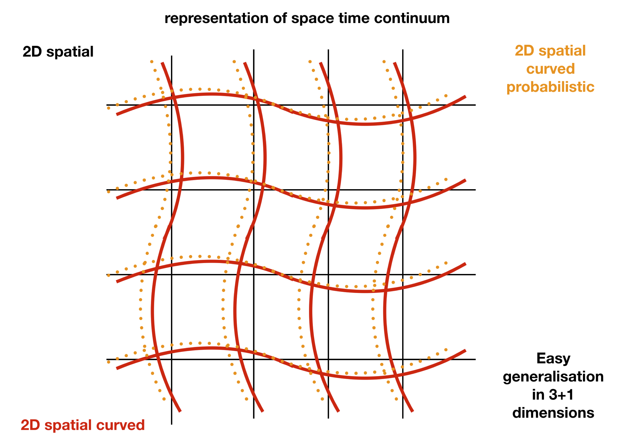
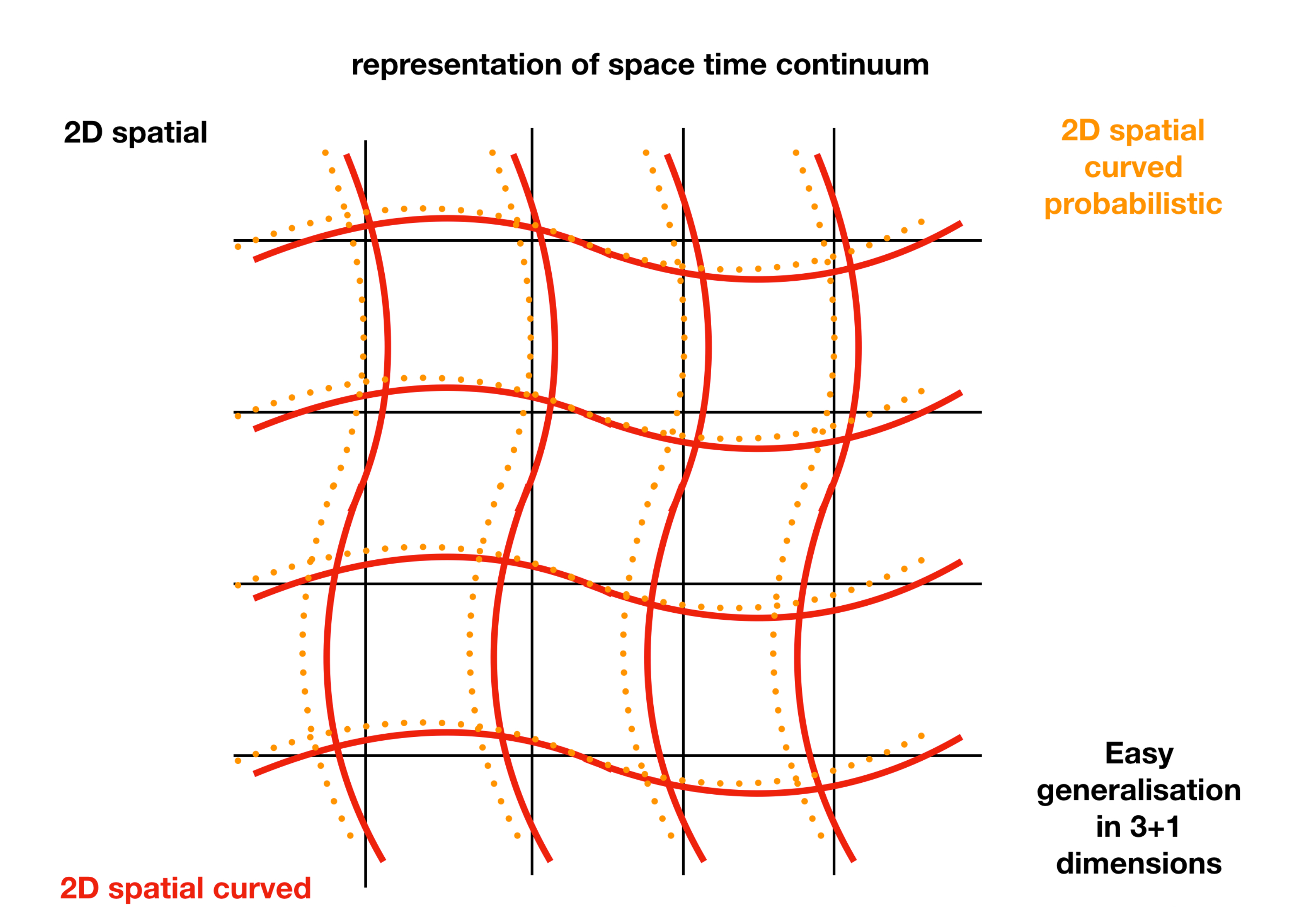
This can be represented graphically in Figure 1. In that figure, we present an example of a 2D space in cartesian coordinates color-coded with black lines. A 2D spacial space which has been curved in the presence of some massive object,color-codedd with red lines, which can be described by the standard Schwarzschild metric, i.e. eq:Schwarzschild. On top of these systems lies a representation of a 2D probabilistic space in the presence of matter, which means it is a spatial space which is both curved and probabilisticcolor-codeded with orange. This metric can be described by the probabilistic Schwarzschild metric, i.e. eq:Schwarzschild3DProb. Therefore, a probabilistic manifold will also have, not only probabilistic properties, but it will also have some additionally nice properties, i.e. locally will look like a Euclidean space.

5.9. Probabilistic Perturbed Einstein-Boltzmann Equations in Conformal Time

In order to build these time of equations we proceed with the following simplification in topological choices and matter-energy species. This means that we are going to derive the simplified probabilistic perturbed Friedmann–Lemaître–Robertson–Walker (sPPFLRW) universe. Note that this section has an overlap with MB95 and some notions from DS21, which we make clear in the text.

Main Theorem

The main theory proved by our study is the following.

Theorem 1. 

Let $({\mathcal{M}}^{(1,3)},m^{\left(\mathrm{sPPFLRW}\right)})$ be a manifold-metric pair of a simplified probabilistic perturbed Friedmann–Lemaître–Robertson–Walker universe. Then by constructing the metric associated with this manifold, using a simple function of conformal time, $P\left(\tau \right)$, implying a metric with a temporal component of a probabilistic nature, then the Einstein-Boltzmann field equations are modified according to this function, $P\left(\tau \right)$, resulting to a probabilistic perturbed expanding universe description.

Proof. 

Note that in section 5.10., we present the constructive choice of a simple probabilistic perturbed expanding manifold-metric pair, while in section 5.11, we present the matter-energy definitions. In section 5.12., we presented the resultant modified Einstein Field Equations. In section 5.13., we present the conservation of energy and the resultant modified Generic Einstein-Boltzmann equations. Sections, Section 5.10 to Section 5.13 present a holistic constructive proof of our main theorem.    □

5.10. Topology Choices

We choose a simpler manifold, in the following sense. In this case, the probabilistic nature appears only in conformal time, not in the spatial space manifold Note that we use the conformal time in order to describe the temporal component. This manifold is denoted with $({\mathcal{M}}^{(1,3)},m^{\left(\mathrm{sPPFLRW}\right)})$. These choices describe a slightly different nature of the spacetime itself and also make the derivation of the relevant equations simpler to handle. The choice of our metric is written as a line element via

$$\begin{array}{c}\hfill d{s}^2=a^2\left(\tau \right)\left[-P^2\left(\tau \right)e^{2\Psi (\tau ,\overrightarrow{x})}d{\tau }^2+e^{-2\Phi (\tau ,\overrightarrow{x})}d{x}^{i}d{x}^j{\delta }_{ij}\right].\end{array}$$

(34)

Our topology choices take into account also a Pseudo Riemannian tensor, ${R^{\mu }}_{\alpha \beta \gamma }$.

5.11. Matter-Energy Definitions

Following MB95, it is convenient to define the over(under)density of any cosmic fluid as,

$$\begin{array}{c}\hfill \delta (\tau ,\overrightarrow{k})\equiv {\displaystyle \frac{\delta \rho (\tau ,\overrightarrow{k})}{\overline{\rho \left(\tau \right)}}}\equiv {\displaystyle \frac{\rho (\tau ,\overrightarrow{k})-\overline{\rho }\left(\tau \right)}{\overline{\rho }\left(\tau \right)}}.\end{array}$$

(35)

This equation will hold for any species of energy in the universe, which the standard ones are cold dark matter (CDM), baryons (b), leptons (ℓ), photons ($\gamma$), neutrinos ($\nu$), dark energy (DE) and/or cosmological constant $\Lambda$. The coordinate velocity, $v_i=d{x}_i/d\tau$ is treated as a perturbation, and we define also the divergence of any fluid in conformal time in Fourier space, as

$$\begin{array}{cc}\hfill \theta & \equiv i{k}^i{v}_i\left(\mathrm{Conformal}\mathrm{Time}\right)\equiv i{k}^i{v}_i\left(\mathrm{Con}\right)\hfill \end{array}$$

(36)

where we have drop the $˜$ symbol for simplicity. Now the energy-stress tensor at first order perturbation is defined as:

$$\begin{array}{cc}\hfill {T^0}_0& =-\rho (\tau ,\overrightarrow{k})=-\left(\overline{\rho }\left(\tau \right)+\delta \rho (\tau ,\overrightarrow{k})\right)\equiv {\overline{T^0}}_0+\delta {T^0}_0=-\overline{\rho }\left(\tau \right)+\delta {T^0}_0\hfill \end{array}$$

(37)

$$\begin{array}{cc}\hfill {T^0}_i& =-\left(\overline{\rho }\left(\tau \right)+\overline{\tilde{P}}\left(\tau \right)\right)v_i\left(\tau \right)=-{T^i}_0=\left(\overline{\rho }\left(\tau \right)+\overline{\tilde{P}}\left(\tau \right)\right)v^i\left(\tau \right)\hfill \end{array}$$

(38)

$$\begin{array}{cc}\hfill {T^i}_j& =\left(\overline{\tilde{P}}\left(\tau \right)+\delta \tilde{P}\left(\tau \right)\right){{\delta }^i}_j+{{\Sigma }^i}_j={{\Sigma }^i}_j,\mathrm{for}i\ne j\hfill \end{array}$$

(39)

$$\begin{array}{cc}\hfill {T^i}_i& =\overline{\tilde{P}}\left(\tau \right)+\delta \tilde{P}\left(\tau \right)={\overline{T^i}}_i+\delta {T^i}_i=\overline{\tilde{P}}\left(\tau \right)+\delta {T^i}_i\hfill \end{array}$$

(40)

where ${{\Sigma }^i}_j$ is the anisotropic stress tensor. Note that, as done in MB95, it is convenient to define $\sigma$ as:

$$(\overline{\rho }+\overline{\tilde{P}})\sigma \equiv -\left[{\widehat{k}}_i{\widehat{k}}^j-{\displaystyle \frac{1}{3}}{{\delta }_i}^j\right]{{\Sigma }^i}_j,$$

(41)

while for $\theta$ it holds that

$$\begin{array}{c}\hfill (\overline{\rho }+\overline{\tilde{P}})\theta =i{k}^j{\delta T^0}_j.\end{array}$$

(42)

Note that we can define the equation of state as $w={\displaystyle \frac{\overline{\tilde{P}}\left(\tau \right)}{\overline{\rho }\left(\tau \right)}},$ and the sound speed of the fluid is defined as $c_s^2={\displaystyle \frac{{{\overline{\tilde{P}}}_s}^{\prime }\left(\tau \right)}{{{\overline{\rho }}_s}^{\prime }\left(\tau \right)}},$ for any species s. Note that for adiabatic perturbations, we do have that ${\displaystyle \frac{\delta \tilde{P}\left(\tau \right)}{\delta \rho \left(\tau \right)}}={\displaystyle \frac{{{\overline{\tilde{P}}}_s}^{\prime }\left(\tau \right)}{{{\overline{\rho }}_s}^{\prime }\left(\tau \right)}}$. It is also convenient to remind the reader the following quantities and identities $v_i=-v^i,q_i=\left(\overline{\rho }+\overline{\tilde{P}}\right)v_i,q_i=-q^i,{T^0}_i=-q_i,{T^0}_i=-{T^i}_0.$

5.12. Einstein Field Equations Choices

Now, by selecting as an input the previous selected topology and the matter-energy definitions to the Einstein Field Equations, i.e. by computing the Christoffel Symbols, the Riemannian Tensor and scalar, as well as the Einstein tensor, we obtain the Einstein Field Equations, $G_{\mu \nu }\propto T_{\mu \nu }$, which are written at 0th order and at first order, as follows. Collectively, we have that the 0th order EFE are

$$\begin{array}{cc}\hfill {\mathcal{H}}^2\left(\tau \right)& ={\displaystyle \frac{8\pi G_{\mathrm{N}}}{3c^4}}{a}^2\left(\tau \right)P^2\left(\tau \right)\overline{\rho }\left(\tau \right)+{\displaystyle \frac{1}{3}}{a}^2\left(\tau \right)P^2\left(\tau \right)\Lambda \hfill \end{array}$$

(43)

$$\begin{array}{cc}\hfill 2{\mathcal{H}}^{\prime }\left(\tau \right)+{\mathcal{H}}^2\left(\tau \right)& =-{\displaystyle \frac{8\pi G_{\mathrm{N}}}{3c^4}}{a}^2\left(\tau \right)P^2\left(\tau \right)\overline{\tilde{P}}\left(\tau \right)+\Lambda a^2\left(\tau \right)P^2\left(\tau \right)\hfill \end{array}$$

(44)

where $\mathcal{H}\left(\tau \right)=a^{\prime }\left(\tau \right)/a\left(\tau \right)$ is the Hubble rate in conformal time. Note that the above set of equations have limit the standard Friedmann equations, for $P\left(\tau \right)\to 1$. Furthermore, the 1st order EFE are

$$\begin{array}{cc}\hfill P^2\left(\tau \right){\displaystyle \frac{k^2}{3}}\Phi \left(\tau ,\overrightarrow{k}\right)+{\mathcal{H}}^2\left(\tau \right)\Psi \left(\tau ,\overrightarrow{k}\right)+\mathcal{H}\left(\tau \right){\Phi }^{\prime }\left(\tau ,\overrightarrow{k}\right)& =-{\displaystyle \frac{4\pi G_{\mathrm{N}}}{3c^4}}{a}^2\left(\tau \right)P^2\left(\tau \right)\overline{\rho }\left(\tau \right)\delta \left(\tau ,\overrightarrow{k}\right)\hfill \\ \hfill {\displaystyle \frac{c^4}{4\pi G_{\mathrm{N}}}}{k}^2\left[{\Phi }^{\prime }\left(\tau ,\overrightarrow{k}\right)+\mathcal{H}\left(\tau \right)\Psi \left(\tau ,\overrightarrow{k}\right)\right]& =a^2\left(\tau \right)P^2\left(\tau \right)\left[\overline{\rho }\left(\tau \right)+\overline{\tilde{P}}\left(\tau \right)\right]\theta \left(\tau \right)\hfill \\ \hfill \left\{2\mathcal{H}\left(\tau \right)\left[3\Phi \left(\tau ,\overrightarrow{k}\right)+2\Psi \left(\tau ,\overrightarrow{k}\right)\right]-\left[{\Phi }^{\prime }\left(\tau ,\overrightarrow{k}\right)-\mathcal{H}\left(\tau \right)\right]\right\}{\displaystyle \frac{P^{\prime }}{P}}& \\ \hfill +\mathcal{H}\left(\tau \right)\left[2{\Phi }^{\prime }\left(\tau ,\overrightarrow{k}\right)+{\Psi }^{\prime }\left(\tau ,\overrightarrow{k}\right)\right]+{\Phi }^{\prime \prime }\left(\tau ,\overrightarrow{k}\right)& \\ \hfill +\left[2{\mathcal{H}}^{\prime }\left(\tau \right)+{\mathcal{H}}^2\left(\tau \right)\right]\Psi \left(\tau ,\overrightarrow{k}\right)+{\displaystyle \frac{1}{3}}{k}^2\left[\Psi \left(\tau ,\overrightarrow{k}\right)-\Phi \left(\tau ,\overrightarrow{k}\right)\right]P^2\left(\tau \right)& ={\displaystyle \frac{4\pi G_{\mathrm{N}}}{3c^4}}{a}^2\left(\tau \right)P^2\left(\tau \right)\delta \tilde{P}\left(\tau \right)\hfill \\ \hfill {\displaystyle \frac{c^4}{12\pi G_{\mathrm{N}}}}{k}^2\left[\Phi \left(\tau ,\overrightarrow{k}\right)-\Psi \left(\tau ,\overrightarrow{k}\right)\right]& =a^2\left(\tau \right)\left[\overline{\rho }\left(\tau \right)+\overline{\tilde{P}}\left(\tau \right)\right]\sigma \hfill \end{array}$$

5.13. Conservation of Matter-Energy and Einstein-Bolzmann Equations

Following MB95, the conservation of matter-energy is usually represented with the conservation of the matter-energy tensor, or the stress energy tensor, via the equations, ${T^{\mu \nu }}_{;\mu }=0$. For completeness note that this section is similar to MB95, except the fact that we denote the new factor $P\left(\tau \right)$, which describes the probabilistic nature of spacetime. We have for the 0th component and the i-component for the 0th order the equations of conservation of matter-energy are

$$\begin{array}{cc}\hfill {\overline{\rho }}_s^{\prime }& =-3\mathcal{H}\left(\tau \right)\left(1+w_s\right){\overline{\rho }}_s\hfill \end{array}$$

(45)

$$\begin{array}{cc}\hfill {\overline{\rho }}_s& =exp\left\{-3\int d\tau {\displaystyle \frac{da\left(\tau \right)/d\tau }{a\left(\tau \right)}}(1+w_s)\right\}\hfill \end{array}$$

(46)

where $w_s={\overline{\tilde{P}}}_s\left(\tau \right)/{\overline{\rho }}_s\left(\tau \right)$. We can assume that $w_{\mathrm{b}}=w_{\mathrm{c}}\simeq 0$, $w_{\gamma }=w_{\nu }\simeq 1/3$, and $w_{\Lambda }\simeq -1$. However, these parameters can be let free and be determined by an experiment.

The matter-energy conservation also implies that we have for the 0th component and the i-component for the 1st order the set of generic Einstein-Boltzmann equations (GEBE for short) as follows.

$$\begin{array}{cc}\hfill {\delta }^{\prime }& =-\left(1+w\right)\left[\theta -3{\Phi }^{\prime }\right]-3{\displaystyle \frac{a^{\prime }}{a}}\left({\displaystyle \frac{\delta \tilde{P}}{\delta \rho }}-w\right)\delta \hfill \end{array}$$

(47)

$$\begin{array}{cc}\hfill {\theta }^{\prime }& =-{\displaystyle \frac{{P\left(\tau \right)}^{\prime }}{P\left(\tau \right)}}\theta -{\displaystyle \frac{a^{\prime }}{a}}(1-3w)\theta -{\displaystyle \frac{w^{\prime }}{1+w}}\theta +{\displaystyle \frac{\delta \tilde{P}/\delta \rho }{1+w}}{k}^2\delta -k^2\sigma +k^2\Psi ,\hfill \end{array}$$

(48)

The aforementioned set of two equations is the modification of the standard conservation of the energy-momentum and mass, by the addition of the term which quantifies the probabilistic nature of the spacetime continuum, by the modification of the divergence of the velocity of of the fluid using the term, $-{\displaystyle \frac{P^{\prime }}{P}}\theta$. Note that GEBE, are called generic, since for its different matter component they take a slightly different form.

Following Ma and Bertschinger [47], 202 [49], we can consider these equations by expressing some relevant quantities, regarding the mass-energy conservations. We denote, $f(\tau ,x^i,\mathfrak{q},{\widehat{\mathfrak{q}}}_j)$, the phase space distribution, where ${\overrightarrow{\mathfrak{q}}}_j=a{\overrightarrow{p}}_j$ is the scaled 3-momentum. The phase space distribution evolves according to Boltzmann equations as

$${\displaystyle \frac{Df}{D\tau }}={\left({\displaystyle \frac{\partial f}{\partial \tau }}\right)}_C$$

(49)

where the left hand side represents terms for the time evolution against the conformal time, $\tau$, without collisions, while the right hand side represent terms for the time evolution with collisions, whose form depends on the nature and type of the particle interactions. Now the left hand side expands according to our variables $(\tau ,x^i,\mathfrak{q},{\widehat{\mathfrak{q}}}_j)$ as

$$\begin{array}{c}\hfill {\displaystyle \frac{Df}{D\tau }}\equiv {\displaystyle \frac{\partial f}{\partial \tau }}+{\displaystyle \frac{d{x}^i}{d\tau }}{\displaystyle \frac{\partial f}{\partial x^i}}+{\displaystyle \frac{d\mathfrak{q}}{d\tau }}{\displaystyle \frac{\partial f}{\partial \mathfrak{q}}}+{\displaystyle \frac{d{\widehat{\mathfrak{q}}}^i}{d\tau }}{\displaystyle \frac{\partial f}{\partial {\widehat{\mathfrak{q}}}^i}}\end{array}$$

(50)

Note that ${\displaystyle \frac{\partial f}{\partial {\widehat{\mathfrak{q}}}^i}}\simeq \mathcal{O}(\Phi ,\Psi )$ is first order while ${\displaystyle \frac{d{\widehat{\mathfrak{q}}}_i}{d\tau }}\simeq \mathcal{O}(\Phi ,\Psi )$ is first order as well, which means we can neglect the ${\displaystyle \frac{d{\widehat{\mathfrak{q}}}^i}{d\tau }}{\displaystyle \frac{\partial f}{\partial {\widehat{\mathfrak{q}}}^i}}\simeq 0$ at first order. The total partial derivative is simplified to

$$\begin{array}{c}\hfill {\displaystyle \frac{Df}{D\tau }}\equiv {\displaystyle \frac{\partial f}{\partial \tau }}+{\displaystyle \frac{d{x}^i}{d\tau }}{\displaystyle \frac{\partial f}{\partial x^i}}+{\displaystyle \frac{d\mathfrak{q}}{d\tau }}{\displaystyle \frac{\partial f}{\partial \mathfrak{q}}}\end{array}$$

(51)

We also assume that the phase space distribution can be written in perturbative form as

$$\begin{array}{c}\hfill f(\tau ,x^i,\mathfrak{q},{\widehat{\mathfrak{q}}}_j)=f_0\left(\mathfrak{q}\right)\left[1+\Xi (\tau ,x^i,\mathfrak{q},{\widehat{\mathfrak{q}}}_j)\right].\end{array}$$

(52)

Note that at first order we have that $\mathcal{O}\left(\Phi \Xi \right)\simeq \mathcal{O}\left(\Psi \Xi \right)\simeq \mathcal{O}\left(\Phi {\partial }_{\mu }\Xi \right)\simeq \mathcal{O}\left(\Psi {\partial }_{\mu }\Xi \right)\simeq \mathcal{O}\left({\partial }_{\mu }\Phi \Xi \right)\simeq \mathcal{O}\left({\partial }_{\mu }\Psi \Xi \right)\simeq 0$, and we have in Fourier space (${\partial }_j\to -i{\overrightarrow{k}}_j$) that the Einstein-Boltzmann Equation for the fluctuations of phase-space energy distribution in a probabilistic perturbed expanding universe are

$$\begin{array}{|c|}\hline \begin{array}{|c|}\hline {\displaystyle \frac{\partial \Xi }{\partial \tau }}-i{\displaystyle \frac{P\left(\tau \right)\mathfrak{q}}{ϵ}}\widehat{\mathfrak{q}}j{\overrightarrow{k}}_j\Xi +\left[{\Phi }^{\prime }+i{\displaystyle \frac{P\left(\tau \right)ϵ}{\mathfrak{q}}}{\widehat{\mathfrak{q}}}^j{\overrightarrow{k}}_j\Psi \right]{\displaystyle \frac{dln{f}_0}{dln\mathfrak{q}}}={\displaystyle \frac{1}{f_0}}{\left({\displaystyle \frac{\partial f}{\partial \tau }}\right)}_C\\ \hline\end{array}\\ \hline\end{array}$$

(53)

where $ϵ$ is the measured energy, defined differently for each particle combination. For massive particles, $ϵ=aE=a\left(\tau \right)\sqrt{{\left(pc\right)}^2+{\left(m{c}^2\right)}^2}$. Note that for $P=1$ we get Eq. 41 from MB95.

Following Ma and Bertschinger [47], 202 [49], note that the Einstein-Boltzmann equations simplify for massless particles. To reduce as much as possible the number of variables we can integrate out the $\mathfrak{q}-$dependence in the massless particle distribution function and expand the angular dependence in a series Legendre polynomials ${\mathcal{P}}_{\ell }\left({\widehat{k}}^i{\widehat{\mathfrak{q}}}_i\right)\equiv {\mathcal{P}}_{\ell }(\widehat{k}·\widehat{\mathfrak{q}})\equiv {\mathcal{P}}_{\ell }\left(\mu \right)$ using the relation

$$\begin{array}{c}\hfill F(\tau ,\overrightarrow{k},\widehat{\mathfrak{q}})={\displaystyle \frac{\int d\mathfrak{q}{\mathfrak{q}}^3{f}_0\left(\mathfrak{q}\right)\Xi }{\int d\mathfrak{q}{\mathfrak{q}}^3{f}_0\left(\mathfrak{q}\right)}}=\sum _{\ell =0}^{\infty }{\left(-i\right)}^{\ell }\left(2\ell +1\right){\left[F_{\nu }\right]}_{\ell }(\tau ,\overrightarrow{k}){\mathcal{P}}_{\ell }(\widehat{k}·\widehat{\mathfrak{q}})\end{array}$$

(54)

The dependence on $\widehat{\mathfrak{q}}$ arises only through $\widehat{k}·\widehat{\mathfrak{q}}$, so that a general distribution may be represented as in latter equation. The factor ${\left(-i\right)}^{\ell }\left(2\ell +1\right)$ is chosen so that the expansion of a plane wave is simplified: $F=e^{-i\overrightarrow{k}·\overrightarrow{x}}$ with $\overrightarrow{x}=r\left(\tau \right)\widehat{x}$ has expansion coefficients the bessel functions, i.e. ${\left[F\right]}_{\ell }=j_{\ell }\left(kr\right)$ .

Now we can apply Eqs. 47, and 53, and we have the following. For cold dark matter species, we have

$$\begin{array}{cc}\hfill {\delta }_{\mathrm{c}}^{\prime }(\tau ,\overrightarrow{k})& =-{\theta }_{\mathrm{c}}(\tau ,\overrightarrow{k})+3{\Phi }^{\prime }(\tau ,\overrightarrow{k})\hfill \end{array}$$

(55)

$$\begin{array}{cc}\hfill {\theta }_{\mathrm{c}}^{\prime }(\tau ,\overrightarrow{k})& =-\left[{\displaystyle \frac{P^{\prime }\left(\tau \right)}{P\left(\tau \right)}}+{\displaystyle \frac{a^{\prime }\left(\tau \right)}{a\left(\tau \right)}}\right]{\theta }_{\mathrm{c}}(\tau ,\overrightarrow{k})+k^2\Psi (\tau ,\overrightarrow{k})\hfill \end{array}$$

(56)

For photon species, we have

$$\begin{array}{cc}\hfill {\delta }_{\gamma }^{\prime }& =-{\displaystyle \frac{4}{3}}{\theta }_{\gamma }+4{\Phi }^{\prime }\hfill \end{array}$$

(57)

$$\begin{array}{cc}\hfill {\theta }_{\gamma }^{\prime }& =-{\displaystyle \frac{P^{\prime }\left(\tau \right)}{P\left(\tau \right)}}{\theta }_{\gamma }+k^2\left[{\displaystyle \frac{1}{4}}{\delta }_{\gamma }-{\sigma }_{\gamma }+\Psi \right]+\alpha n_l{\sigma }_T({\theta }_b-{\theta }_{\gamma })\hfill \end{array}$$

(58)

$$\begin{array}{cc}\hfill F_{\gamma 2}^{\prime }& =2{\sigma }_{\gamma }^{\prime }=\left[{\displaystyle \frac{8P\left(\tau \right)}{15}}{\theta }_{\gamma }-{\displaystyle \frac{3P\left(\tau \right)k}{5}}{F}_{\gamma 3}\right]-\alpha n_l{\sigma }_T{\displaystyle \frac{9}{5}}{\sigma }_{\gamma }+\alpha n_l{\sigma }_T{\displaystyle \frac{1}{10}}\left(G_{\gamma 0}+G_{\gamma 2}\right)\hfill \end{array}$$

(59)

$$\begin{array}{cc}\hfill F_{\gamma \ell }^{\prime }& ={\displaystyle \frac{P\left(\tau \right)k}{2\ell +1}}\left[\ell F_{\gamma (\ell -1)}-(\ell +1)F_{\gamma (\ell +1)}\right]-\alpha n_l{\sigma }_T{F}_{\gamma \ell },\ell \ge 3\hfill \end{array}$$

(60)

$$\begin{array}{cc}\hfill G_{\gamma \ell }^{\prime }& ={\displaystyle \frac{P\left(\tau \right)k}{2\ell +1}}\left[\ell G_{\gamma (\ell -1)}-(\ell +1)G_{\gamma (\ell +1)}\right]+\alpha n_l{\sigma }_T\left[-G_{\gamma \ell }+{\displaystyle \frac{1}{2}}\left(F_{\gamma 2}+G_{\gamma 0}+G_{\gamma 2}\right)({\delta }_{\ell 0}+{\delta }_{\ell 2}{\displaystyle \frac{1}{5}})\right]\hfill \end{array}$$

(61)

where $F_{\gamma \ell }$ are the perturbation of the energy distribution of photons in a particular harmonic expansion, $G_{\gamma \ell }$ are the perturbation of the energy distribution of the polarisation of photons in a particular harmonic expansion, and $\left\{F_{\gamma 1},F_{\gamma 2}\right\}=\left\{{\displaystyle \frac{4{\theta }_{\gamma }}{3k}},2{\sigma }_{\gamma }\right\}$. The truncation of the last two equations become the constraints

$$\begin{array}{cc}\hfill F_{\gamma {\ell }_{\max }}^{\prime }& =P\left(\tau \right)k\left[\ell F_{\gamma {\ell }_{\max }-1}-{\displaystyle \frac{({\ell }_{\max }+1)}{k\tau }}{F}_{\gamma {\ell }_{\max }}\right]-\alpha n_l{\sigma }_T{F}_{\gamma {\ell }_{\max }},\ell \ge 3\hfill \end{array}$$

(62)

$$\begin{array}{cc}\hfill G_{\gamma {\ell }_{\max }}^{\prime }& =P\left(\tau \right)k\left[\ell G_{\gamma ({\ell }_{\max }-1)}-{\displaystyle \frac{({\ell }_{\max }+1)}{k\tau }}{G}_{\gamma \left({\ell }_{\max }\right)}\right]-\alpha n_l{\sigma }_T{G}_{\gamma {\ell }_{\max }}\hfill \end{array}$$

(63)

Note that there is a momentum transfer from the baryons into the photon species which is represented via the term $\alpha n_l{\sigma }_T({\theta }_{\gamma }-{\theta }_b)$, in Eqs. and .

For collisionless, massless neutrini species, we have

$$\begin{array}{cc}\hfill {\delta }_{\nu }^{\prime }& =-{\displaystyle \frac{4}{3}}{\theta }_{\nu }+4{\Phi }^{\prime }\hfill \end{array}$$

(64)

$$\begin{array}{cc}\hfill {\theta }_{\nu }^{\prime }& =-{\displaystyle \frac{P^{\prime }\left(\tau \right)}{P\left(\tau \right)}}{\theta }_{\nu }+k^2\left[{\displaystyle \frac{1}{4}}{\delta }_{\nu }-{\sigma }_{\nu }+\Psi \right]\hfill \end{array}$$

(65)

$$\begin{array}{cc}\hfill F_{\nu \ell }^{\prime }& ={\displaystyle \frac{P\left(\tau \right)k}{2\ell +1}}\left[\ell F_{\nu (\ell -1)}-(\ell +1)F_{\nu (\ell +1)}\right],\ell \ge 2\hfill \end{array}$$

(66)

while the truncation of the last equations becomes the constraint

$$\begin{array}{cc}\hfill F_{\nu ({\ell }_{\max }+1)}& \approx {\displaystyle \frac{2{\ell }_{\max }+1}{P\left(\tau \right)k\tau }}{F}_{\nu {\ell }_{\max }}-F_{\nu ({\ell }_{\max }-1)}.\hfill \end{array}$$

(67)

For baryon and leptons species (which we consider as a baryon species, since the baryons are way more than the leptons), we have

$$\begin{array}{cc}\hfill {\delta }_b^{\prime }& =-{\theta }_b+3{\Phi }^{\prime }\hfill \end{array}$$

(68)

$$\begin{array}{cc}\hfill {\theta }_b^{\prime }& =-{\displaystyle \frac{P^{\prime }\left(\tau \right)}{P\left(\tau \right)}}{\theta }_b-\mathcal{H}{\theta }_b+c_s^2{k}^2{\delta }_b+k^2\Psi +{\displaystyle \frac{4{\overline{\rho }}_b}{3{\overline{\rho }}_{\gamma }}}\alpha n_l{\sigma }_T({\theta }_{\gamma }-{\theta }_b)\hfill \end{array}$$

(69)

The squared baryon sound speed is considered to be

$$\begin{array}{c}\hfill c_s^2={\displaystyle \frac{{\overline{\tilde{P}}}_b^{\prime }}{{\overline{\rho }}_b^{\prime }}}={\displaystyle \frac{k_B{T}_b}{{\mu }_{\mathrm{mol}}}}\left(1-{\displaystyle \frac{1}{3}}{\displaystyle \frac{dln{T}_b}{dln\alpha }}\right)\end{array}$$

(70)

where ${\mu }_{\mathrm{mol}}$ is the mean molecular weight which includes free leptons and all ions of H to He. In the last equality, we assume that the mean molecular weight slowly varies with time. This approximation holds, since even during recombination, ${\mu }_{\mathrm{mol}}^{\prime }$ is maximum and the baryons minorly contribute to the pressure of the baryon-photon fluid. The baryon temperature evolution is given by

$$T_b^{\prime }=-2\mathcal{H}+{\displaystyle \frac{8}{3}}{\displaystyle \frac{{\mu }_{\mathrm{mol}}}{m_l}}{\displaystyle \frac{{\overline{\rho }}_{\gamma }}{{\overline{\rho }}_b}}\alpha n_l{\sigma }_T(T_{\gamma }-T_b),$$

(71)

where $\alpha$ is the fine structure constant. The lepton-ion collisions are rapid enough to admit kinetic equilibrium which holds with a common temperature for leptons and baryons, $T_l=T_b$. The eq:baryontemperatureevolution occurs from the first law of thermodynamics which states that the internal energy transferred as heat, Q, for baryons and photons varies as $dQ={\displaystyle \frac{3}{2}}d\left({\displaystyle \frac{{\overline{\tilde{P}}}_b}{{\overline{\rho }}_b}}\right)+{\tilde{P}}_{b}d\left({\overline{\rho }}_b^{-1}\right)$ with a heating rate ${\displaystyle \frac{dQ}{d\tau }}=4{\displaystyle \frac{{\overline{\rho }}_{\gamma }}{{\overline{\rho }}_b}}\alpha n_l{\sigma }_T{k}_B\left(T_{\gamma }-T_b\right),$ where ${\sigma }_T$ is the Thomson scattering, and $k_B$ is the Boltzmann constant.

Note that the proper time derivative of the ratio of photon density to baryon density, $R_{\gamma \to b}=4{\overline{\rho }}_{\gamma })/\left(3{\overline{\rho }}_b\right)$, is

$${\partial }_{\tau }{R}_{\gamma \to b}=-R_{\gamma \to b}{\displaystyle \frac{a^{\prime }}{a}}$$

(72)

Note that Thomson opacity, $o_T\equiv \alpha n_l{\sigma }_T$, can be large enough that photons and baryons are tightly coupled in coupling time, ${\tau }_{\mathrm{c}}$, which is defined given by

$$\begin{array}{c}\hfill {\tau }_{\mathrm{c}}=o_T^{-1}={\displaystyle \frac{1}{\alpha n_l{\sigma }_T}}.\end{array}$$

(73)

We also assume that the gas is fully ionised which means that the lepton density is $n_l\propto a^{-3}\left(\tau \right)$, in turn this means that he coupling time can be approximated as

$$\begin{array}{cc}\hfill {\tau }_{\mathrm{c}}& \propto a^{+3},{\partial }_{\tau }{\tau }_{\mathrm{c}}=3a^{-1}\left(\tau \right){\tau }_{\mathrm{c}}.\hfill \end{array}$$

(74)

We also assume that the baryon temperature is approximately the radiation temperature, which means that the sound speed is approximated as

$$\begin{array}{cc}\hfill c_s^2& \propto a^{-1},{\partial }_{\tau }\left(c_s^2\right)=-{\displaystyle \frac{a^{\prime }}{a}}{c}_s^2.\hfill \end{array}$$

(75)

Finally we define the ratio of neutrini density to radiation density as

$$\begin{array}{c}\hfill R_{\nu \to r}={\overline{\rho }}_{\gamma }/{\overline{\rho }}_r={\overline{\rho }}_{\nu }/({\overline{\rho }}_{\nu }+{\overline{\rho }}_{\gamma }).\end{array}$$

(76)

In summary, under reasonable assumptions following by our application of probabilistic dimensions on the machinary introduced in MB95 and DS21, regarding the matter evolution in a probabilistic spacetime, the initial conditions are given by the following set of equation, which determine the initial conditions

$$\begin{array}{cc}\hfill P\left({\tau }_{\mathrm{i}}\right)& \approx P_{\mathrm{constant}}\equiv {\tau }_{\mathrm{i}}^{-1}\in \mathbb{R}\hfill \end{array}$$

(77)

$$\begin{array}{cc}\hfill \Psi ({\tau }_i,k)& \approx {\displaystyle \frac{20C}{15+4R_{\nu \to r}}}\in \mathbb{R}\hfill \end{array}$$

(78)

$$\begin{array}{cc}\hfill \Phi ({\tau }_i,k)& \approx \left(1+{\displaystyle \frac{2}{5}}{R}_{\nu \to r}\right)\Psi ({\tau }_{\mathrm{i}},k)\in \mathbb{R}\hfill \end{array}$$

(79)

$$\begin{array}{cc}\hfill {\theta }_{\gamma }& \approx {\theta }_{\nu }\approx {\theta }_c\approx {\theta }_b\approx {\displaystyle \frac{10C}{15+4R_{\nu \to r}}}{k}^2{P}^{-1}\left(\tau \right)\approx {\displaystyle \frac{1}{2}}{k}^2\tau \Psi ({\tau }_{\mathrm{i}},k)\in {\mathbb{R}}^{D_k+D_{\tau }}\hfill \end{array}$$

(80)

$$\begin{array}{cc}\hfill {\delta }_{\gamma }& \approx -{\displaystyle \frac{40C}{15+4R_{\nu \to r}}}=-2\Psi ({\tau }_i,k)\in \mathbb{R}\hfill \end{array}$$

(81)

$$\begin{array}{cc}\hfill {\delta }_c& \approx {\delta }_b\approx {\displaystyle \frac{3}{4}}{\delta }_{\nu }\approx {\displaystyle \frac{3}{4}}{\delta }_{\gamma }\in \mathbb{R}\hfill \end{array}$$

(82)

$$\begin{array}{cc}\hfill {\sigma }_{\nu }& \approx {\displaystyle \frac{4C}{3(15+4R_{\nu \to r})}}{k}^2{P}^{-2}\left(\tau \right)={\displaystyle \frac{2}{15}}{k}^2{\tau }^2\Psi ({\tau }_{\mathrm{i}},k)\in {\mathbb{R}}^{D_k+D_{\tau }}\hfill \end{array}$$

(83)

where $D_k$ and $D_{\tau }$ are the dimensions of the binned observed k wavevector magnitude, and the conformal time, respectively. Note that this solution also means that

$$\begin{array}{c}\hfill P\sim {\tau }^{-1},P^{\prime }\sim -{\tau }^{-2},{\displaystyle \frac{P^{\prime }}{P}}\sim -{\tau }^{-1}\sim -P\sim -\mathcal{H}\sim -{\displaystyle \frac{a^{\prime }}{a}},\end{array}$$

(84)

while initially, we have

$$\begin{array}{c}\hfill P\sim P_{\mathrm{constant}},P^{\prime }\sim 0.\end{array}$$

(85)

Therefore, in order to solve the GEBE, we need to define the $(k,\tau )$ dependence of the potential, $\Psi$, as

$$\Psi (\tau ,k)={\displaystyle \frac{15+4R_{\nu \to r}}{20C}}\Psi ({\tau }_i,k).$$

(86)

This means that C and $\Psi (\tau ,k)$, is left to be determined from the numerical solutions of GEBE, with initial conditions the set of Eqs. 77-86.

6. Spacion: From Graviton to Probablon, to Informaton

The standard cosmological model, which is based on GR and perturbation theory, basically constructs a spacetime in which its perturbation already assumes gravitational waves. This simply means that there is potentially the graviton particle-wave or graviton field, and the cold dark matter field. However, having aside the dark matter, the graviton field notion means that the particle-wave duality is already inherent in GR and the SMC, even though such particles have not been detected, yet. By introducing the probabilistic concept in perturbed spacetime, we discover another more concrete property of the wave-particle duality to the graviton, which is the probabilistic or informatic nature of such graviton. This kind of discovery is similar to concepts introduced by quantum field theory. QFT introduces the concept of probabilistic notions to the all elementary particles. To extend, we introduced another abstract useful concept. Note that motivated by generic arguments, we can also distinguish several kinds of properties to elementary particles or fields, by introducing compound words which have not been discussed yet in the literature. These compound words achieve to generate the distinction between the different properties of the fields and they are essential to our understanding of nature.

Motivated by generic arguments of probabilities, an elementary particle which possesses probabilistic properties, would be named probablon or probablion. We continue with the probablon term since it is both euphonic and a simpler nomenclature. So far these kinds of particles have been mapped by physicists, and they are the well-known elementary particles, the quarks, leptons, bosons, and fermions, which all share probabilistic notions. However, the probablon category of elementary particles generalises the notion of elementary particles, in the sense that there are elementary particles which possess a probabilistic nature and those which have no such nature. So far nature shows that most elementary particles possess kinds of probabilistic properties, such as the ones which are inherited by QFT.

We also introduce here the concept of the probabilistic graviton, which is the graviton with further probabilistic notions as the ones we have described before. Note that the graviton is basically a spacetime particle, and therefore it is crucial to distinguish that the graviton particle bears its name historically since it was a particle which resulted from the description of gravity. However, since it has properties of spacetime, then we can also make up the name for such particle, namely the spacetimion. Motivated by this distinction, we generalise another notion of particles, i.e. the notion of spacion, spatiallion and the timion. A spacion is a particle which has the generic property which states that this particle belongs to a generic space and not a specific space, the spacetime. While the spatiallion has a generic property, the property of spatial space, the timion has the property of time. To explain more deeply these kinds of particles, one needs to think that if a particle has the space property, then this means that this particle exists in a space. This is a very basic generic property, which most known particles have, this property was not highlighted yet. For example, every particle field exists in a generic space, and therefore it belongs to the category of spacions. Furthermore, we can think of the probabilistic notions that space has, we can think of another compound particle which exists in a space with probabilistic properties. These kinds of particles would be called probablispacion. Consequently, a particle, which has probabilistic notions and notions of spacetime, would be called probablispacetimion, which is a clearer name than what we have called graviton in the first place.

Along these lines, we also introduce the concept of the informaton. Informaton is any particle or field which possess an information of any kind. Note that a spacion, a probablon contains also information, and it can be considered as a informaton as well. The elementary particles possess also information about their mass, charge, or spin, and therefore they also considered as informatons. Then we can also built the compound objects which are the informatimion (possessing properties of informaton and timion), informatic graviton (informaton and graviton), probablinformaton (probablon and informaton).

Since these concepts are introduced in the literature, it is timely, reasonable, and plausible to ask ourselves, are all elementary particles possess all these kinds of properties, as they have been introduced by quantum field theory and gravity using perturbation theory, or are there new classes of particles which we have yet to discover, kinds of particles that not all of them have these kinds of properties ?

In summary, novel particles introduced in this study are the spacion, spatiallion, timion, informaton, probablon, as well as compounds, such as spacetimion, probablispacion, probablispacetimion, probabilistic graviton by analysing further the graviton concept. Note that we have merely touched describing the properties of such particles, but it is important to make such distinction, at least at the philosophical level, before starting seriously searching for such particles. We leave an extension of this discussion, its implications, and applications to a future study.

7. An Interesting Outlook

The answers, which we have provided with this study, have inspired the following interesting and challenging questions which can be answered in the future. Here we give a brief outlook, in which we suggest a way to combine novel concepts with older ones in the future, to satisfy our quest for an even better and more appropriate description of our universe. The questions which are inspired by this study are the following: How can we more properly, appropriately, and mathematically write the gravity action, i.e. the general relativity or a more sophisticated system such as the one from Horndeski action, in a probabilistic frame study ?; What is the entropy in a probabilistic spacetime and how can we define it ?; What is the entropy of probabilistic actions and how can we define it?; Is there any more fundamental mechanism producing the probabilistic nature of spacetime other than a mathematical consistency ?; What is the description of gravitational waves in a probabilistic spacetime ? Could the Higgs field, Higgs [29], Higgs [30], and any of the other elementary particles or black holes be described in a probabilistic spacetime ?; How AdS/CFT correspondence can be enriched from the perspective of probabilistic dimensions ?; What is the essence of supergravity in a probabilistic spacetime frame study ? Are there probabilistic super-particles ? Having written a gravity action in terms of a probabilistic spacetime, can we reconcile quantum gravity by quantising the probabilistic gravity Ali and Engliš [59] ?; How, can we reconcile other recently developed models of modified gravity, such as the ones listed in Clifton et al. [32], Koyama [33], Ezquiaga and Zumalacárregui [34], Ntelis and Morris [35] ?; How probabilistic manifold-metric pairs change our description for black hole/string transition Chen et al. [60] ? Can we build a multi-gravity using the probabilistic dimensions ?; Are the extra dimensions, which are predicted by string theory, hidden in the probabilistic dimensions ?; Can we provide a better description of the large-scale structure, using the probabilistic spaces and dimensions ?; Is there a better description of the multiverse, in which probabilistic dimensions play an important role ?; Are there large-scale structures in the frame study of the multiverse ? We leave the answers to these interesting questions for a future study.

8. Summary, Conclusion and Discussion

With this study, we open up further the possibility of probabilistic spacetimes and we do the first steps of creating a probabilistic gravity, i.e. the first steps towards a description of a probabilistic universe. We have simply revised the notions of probabilities in differential geometry and topology. We have generalised the notion of a dimension to a dimension which does not simply exist, but there is a whole set of dimensions, from which some events of the existence of a dimension rises with some probability, which might depend on time, space, and/or energy. We have rewritten general relativity in terms of a probabilistic spacetime. We have introduced the concept of a probabilistic spacetime in several metrics of expanding universes. We have considered a probabilistic space-time in the presence of some massive objects. We have also considered a simple combination of a probabilistic expanding spacetime in the presence of some massive objects. These answers result in toy models for probabilistic gravity and a probabilistic expanding universe. Finally we have introduced novel type of particles or fields such as the spacion, spatiallion, timion, informaton, probablon, and probabilistic graviton, among others.

These answers inspired the following interesting and challenging questions, which summarise as follows: How can we more properly, appropriately, and mathematically write the gravity action, i.e. the general relativity one or more sophisticated ones, in a probabilistic frame study ?; What is the entropy in a probabilistic spacetime and how can we define it ?; What is the entropy of probabilistic actions and how can we define it?; Is there any more fundamental mechanism producing the probabilistic nature of spacetime other than a mathematical consistency ?; What is the description of gravitational waves in a probabilistic spacetime ?; Could the Higgs [29], Higgs [30]-field and any of the other elementary particles or black holes be described in a probabilistic spacetime ?; How AdS/CFT correspondence can be enriched from the perspective of probabilistic dimensions ?; Are the extra dimensions, which are predicted by string theory, hidden in the probabilistic dimensions ?; Having written a gravity action in terms of a probabilistic spacetime, can we reconcile quantum gravity by quantising the probabilistic gravity Ali and Engliš [59] ? We leave the answers to these interesting questions for a future study. Our present is brighter and our future is fruitful, promising and full of surprises in which answers will be given to these questions.

                                 Ó$\pi ϵ\rho$É$\delta ϵ\iota \Delta ϵ\tilde{\iota }\xi \alpha \iota$

Appendix A.1. General Covariance of the EFE

The Einstein Field Equations are:

$$G_{\mu \nu }+\Lambda g_{\mu \nu }={\displaystyle \frac{8\pi G}{c^4}}{T}_{\mu \nu }$$

where:

• $G_{\mu \nu }=R_{\mu \nu }-{\displaystyle \frac{1}{2}}R{g}_{\mu \nu }$ is the Einstein tensor,
• $R_{\mu \nu }$ is the Ricci curvature tensor,
• R is the Ricci scalar,
• $g_{\mu \nu }$ is the metric tensor,
• $\Lambda$ is the cosmological constant,
• $T_{\mu \nu }$ is the stress-energy tensor.

The tensors $G_{\mu \nu }$, $g_{\mu \nu }$, and $T_{\mu \nu }$ transform according to the rules of tensor calculus under any smooth coordinate transformation, ensuring the general covariance of the EFE.

Appendix A.2. The Probabilistic Expanding Metric

The infinitesimal element of the probabilistic expanding metric in comoving coordinates and conformal time is:

$$d{s}^2=a^2\left(\tau \right)\left[-P^2\left(\tau \right)d{\tau }^2+d{\overrightarrow{x}}^2\right]$$

where

$$g_{\mu \nu }=\left[\begin{array}{cccc}-a^2\left(\tau \right)P^2\left(\tau \right)& 0& 0& 0\\ 0& a^2\left(\tau \right)& 0& 0\\ 0& 0& a^2\left(\tau \right)& 0\\ 0& 0& 0& a^2\left(\tau \right)\end{array}\right]$$

Note that we can also consider the simplest perturbed probabilistic expanding metric, in which case, the infinitesimal element is

$$d{s}^2=a^2\left(\tau \right)\left[-P^2\left(\tau \right)e^{\Psi (\tau ,\overrightarrow{x})}d{\tau }^2+e^{-\Phi (\tau ,\overrightarrow{x})}d{\overrightarrow{x}}^2\right]$$

where

$$g_{\mu \nu }=\left[\begin{array}{cccc}-a^2\left(\tau \right)P^2\left(\tau \right)e^{\Psi (\tau ,\overrightarrow{x})}& 0& 0& 0\\ 0& a^2\left(\tau \right)e^{-\Phi (\tau ,\overrightarrow{x})}& 0& 0\\ 0& 0& a^2\left(\tau \right)e^{-\Phi (\tau ,\overrightarrow{x})}& 0\\ 0& 0& 0& a^2\left(\tau \right)e^{-\Phi (\tau ,\overrightarrow{x})}\end{array}\right]$$

Appendix A.3. Coordinate Transformations and Tensorial Nature

Let’s consider a general smooth coordinate transformation $x^{{\mu }^{\prime }}=x^{{\mu }^{\prime }}\left(x^{\nu }\right)$, of the two metrics, expressed in the previous section, sec:probabilisticexpandingconformaltimemetric. Under this transformation, tensors transform as follows:

• The metric tensor transforms as:

  $$g_{{\mu }^{\prime }{\nu }^{\prime }}={\displaystyle \frac{\partial x^{\mu }}{\partial x^{{\mu }^{\prime }}}}{\displaystyle \frac{\partial x^{\nu }}{\partial x^{{\nu }^{\prime }}}}{g}_{\mu \nu }$$
• The Ricci tensor transforms as:

  $$R_{{\mu }^{\prime }{\nu }^{\prime }}={\displaystyle \frac{\partial x^{\mu }}{\partial x^{{\mu }^{\prime }}}}{\displaystyle \frac{\partial x^{\nu }}{\partial x^{{\nu }^{\prime }}}}{R}_{\mu \nu }$$
• The Ricci scalar transforms as:

  $$R^{\prime }=R$$
• The stress-energy tensor transforms as:

  $$T_{{\mu }^{\prime }{\nu }^{\prime }}={\displaystyle \frac{\partial x^{\mu }}{\partial x^{{\mu }^{\prime }}}}{\displaystyle \frac{\partial x^{\nu }}{\partial x^{{\nu }^{\prime }}}}{T}_{\mu \nu }$$

Appendix A.4. Preservation of the EFE Under Coordinate Transformations

Since the EFE are tensor equations, their form is preserved under coordinate transformations. Explicitly, under a coordinate transformation $x^{\mu }\to x^{{\mu }^{\prime }}\left(x^{\nu }\right)$, the EFE transform as:

$$G_{{\mu }^{\prime }{\nu }^{\prime }}+\Lambda g_{{\mu }^{\prime }{\nu }^{\prime }}={\displaystyle \frac{8\pi G}{c^4}}{T}_{{\mu }^{\prime }{\nu }^{\prime }}$$

Given the transformation properties of the tensors, we have:

$$\begin{array}{cc}\hfill \left({\displaystyle \frac{\partial x^{\mu }}{\partial x^{{\mu }^{\prime }}}}{\displaystyle \frac{\partial x^{\nu }}{\partial x^{{\nu }^{\prime }}}}{G}_{\mu \nu }\right)+\Lambda \left({\displaystyle \frac{\partial x^{\mu }}{\partial x^{{\mu }^{\prime }}}}{\displaystyle \frac{\partial x^{\nu }}{\partial x^{{\nu }^{\prime }}}}{g}_{\mu \nu }\right)& ={\displaystyle \frac{8\pi G}{c^4}}\left({\displaystyle \frac{\partial x^{\mu }}{\partial x^{{\mu }^{\prime }}}}{\displaystyle \frac{\partial x^{\nu }}{\partial x^{{\nu }^{\prime }}}}{T}_{\mu \nu }\right)\hfill \end{array}$$

(A1)

$$\begin{array}{cc}\hfill \left({\displaystyle \frac{\partial x^{\mu }}{\partial x^{{\mu }^{\prime }}}}{\displaystyle \frac{\partial x^{\nu }}{\partial x^{{\nu }^{\prime }}}}\right)\left(G_{\mu \nu }+\Lambda g_{\mu \nu }\right)& =\left({\displaystyle \frac{\partial x^{\mu }}{\partial x^{{\mu }^{\prime }}}}{\displaystyle \frac{\partial x^{\nu }}{\partial x^{{\nu }^{\prime }}}}\right)\left({\displaystyle \frac{8\pi G}{c^4}}{T}_{\mu \nu }\right)\hfill \end{array}$$

(A2)

$$\begin{array}{cc}\hfill G_{\mu \nu }+\Lambda g_{\mu \nu }& ={\displaystyle \frac{8\pi G}{c^4}}{T}_{\mu \nu }\hfill \end{array}$$

(A3)

Since the transformation properties hold, the EFE remain valid in the new coordinate system.

References

- Polyakov, A.M. Quantum geometry of bosonic strings. Physics Letters B 1981, 103, 207–210. [Google Scholar] [CrossRef]
- Deser, S.; Zumino, B. Consistent Supergravity. Phys. Lett. B 1976, 62, 335. [Google Scholar] [CrossRef]
- Seiberg, N.; Witten, E. String theory and noncommutative geometry. JHEP 1999, 09, 032. [Google Scholar] [CrossRef]
- Seiberg, N.; Witten, E. String theory and noncommutative geometry. Journal of High Energy Physics 1999, 1999, 032. [Google Scholar] [CrossRef]
- Witten, E. Perturbative gauge theory as a string theory in twistor space. Commun. Math. Phys. 2004, 252, 189–258. [Google Scholar] [CrossRef]
- Rovelli, C. Quantum gravity; Cambridge Monographs on Mathematical Physics, Univ. Pr.: Cambridge, UK, 2004. [Google Scholar] [CrossRef]
- Maldacena, J. The Large-N Limit of Superconformal Field Theories and Supergravity. International Journal of Theoretical Physics 1999, 38, 1113–1133. [Google Scholar] [CrossRef]
- Witten, E. Anti-de Sitter space and holography. Advances in Theoretical and Mathematical Physics 1998, 2, 253–291. [Google Scholar] [CrossRef]
- Amendola, L. Coupled quintessence. Phys. Rev. D 2000, 62, 043511. [Google Scholar] [CrossRef]
- D’Amico, G.; Kaloper, N. Rollercoaster Cosmology. arXiv e-prints, arXiv:2011.09489, [arXiv:hep-th/2011.09489].
- Susskind, L. The world as a hologram [11]. Journal of Mathematical Physics 1995, 36, 6377–6396. [Google Scholar] [CrossRef]
- Chen, Y.; Maldacena, J. String scale black holes at large D. arXiv e-prints, arXiv:2106.02169, [arXiv:hep-th/2106.02169].
- Carroll, S.M. Reality as a Vector in Hilbert Space. arXiv e-prints, arXiv:2103.09780, [arXiv:quant-ph/2103.09780].
- Ntelis, P. A Dt,Dx manifolds of Nt-objects with and without contaminants. In preparation.
- Anchordoqui, L.A.; Antoniadis, I. Large extra dimensions from higher-dimensional inflation 2023. arXiv:hep-ph/2310.20282].
- Enßlin, T. Information field theory. AIP Conference Proceedings 2013, 1553, 184–191. [Google Scholar] [CrossRef]
- Planck Collaboration. ; Aghanim, N.; Akrami, Y.; Ashdown, M.; Aumont, J.; Baccigalupi, C.; Ballardini, M.; Banday, A.J.; Barreiro, R.B.; Bartolo, N.; et al. Planck 2018 results. VI. Cosmological parameters. 2020, arXiv:astro-ph.CO/1807.06209]641, A6. [CrossRef]
- eBOSS Collaboration. ; Alam, S.; Aubert, M., Avila, S., Balland, C., Bautista, J.E., Bershady, M.A., Bizyaev, D., Blanton, M.R., Bolton, A.S., Eds.; et al. The Completed SDSS-IV extended Baryon Oscillation Spectroscopic Survey: Cosmological Implications from two Decades of Spectroscopic Surveys at the Apache Point observatory. arXiv e-prints 2020, p. arXiv:2007.08991, [arXiv:astro-ph.CO/2007. [Google Scholar]
- Abbott, B.P.; Abbott, R.; Abbott, T.D.; Abernathy, M.R.; Acernese, F.; Ackley, K.; Adams, C.; Adams, T.; Addesso, P.; Adhikari, R.X.; et al. Observation of Gravitational Waves from a Binary Black Hole Merger. Phys. Rev. Lett. 2016, 116, 061102. [Google Scholar] [CrossRef] [PubMed]
- Zyla, P.; et al. Review of Particle Physics. PTEP 2020, 2020, 083C01. [Google Scholar] [CrossRef]
- Carroll, S.M.; Press, W.H.; Turner, E.L. The cosmological constant. 1992, 30, 499–542. [CrossRef]
- Carroll, S.M. The Cosmological Constant. Living Reviews in Relativity 2001, 4, 1. [Google Scholar] [CrossRef]
- Bernardeau, F.; Colombi, S.; Gaztañaga, E.; Scoccimarro, R. Large-scale structure of the Universe and cosmological perturbation theory. 2002, 367, 1–248, [arXiv:astro-ph/astro-ph/0112551]. [CrossRef]
- Lombriser, L. On the cosmological constant problem. Physics Letters B 2019, arXiv:gr-qc/1901.08588]797, 134804. [Google Scholar] [CrossRef]
- Linder, E.V. What is the Standard Cosmological Model? 5 arXiv:astro-ph.CO/2105.02903], 2021.
- Guth, A.H.; Pi, S.Y. Fluctuations in the New Inflationary Universe. Phys. Rev. Lett. 1982, 49, 1110–1113. [Google Scholar] [CrossRef]
- Starobinsky, A.A. Dynamics of phase transition in the new inflationary universe scenario and generation of perturbations. Physics Letters B 1982, 117, 175–178. [Google Scholar] [CrossRef]
- Linde, A.D. A new inflationary universe scenario: A possible solution of the horizon, flatness, homogeneity, isotropy and primordial monopole problems. Physics Letters B 1982, 108, 389–393. [Google Scholar] [CrossRef]
- Higgs, P.W. Broken symmetries, massless particles and gauge fields. Phys. Lett. 1964, 12, 132–133. [Google Scholar] [CrossRef]
- Higgs, P.W. Broken Symmetries and the Masses of Gauge Bosons. Phys. Rev. Lett. 1964, 13, 508–509. [Google Scholar] [CrossRef]
- Englert, F.; Brout, R. Broken Symmetry and the Mass of Gauge Vector Mesons. Phys. Rev. Lett. 1964, 13, 321–323. [Google Scholar] [CrossRef]
- Clifton, T.; Ferreira, P.G.; Padilla, A.; Skordis, C. Modified gravity and cosmology. 513, arXiv:astro-ph.CO/1106.2476]. [CrossRef]
- Koyama, K. Cosmological tests of modified gravity. Reports on Progress in Physics 2016, arXiv:astro-ph.CO/1504.04623]79, 046902. [Google Scholar] [CrossRef] [PubMed]
- Ezquiaga, J.M.; Zumalacárregui, M. Dark energy after GW170817: dead ends and the road ahead. Physical review letters 2017, 119, 251304. [Google Scholar] [CrossRef]
- Ntelis, P.; Morris, A. Functors of Actions. Foundations of Physics 2023, 53, 29. [Google Scholar] [CrossRef]
- Bianchi, L. Sugli spazi a tre dimensioni che ammettono un gruppo continuo di movimenti. Memorie della Societa Italiana delle Scienze. detta dei XL.(3) 1897, 11, 267–352. [Google Scholar]
- Menger, K. Statistical Metrics. Proceedings of the National Academy of Sciences 1942, 28, 535–537. [Google Scholar] [CrossRef]
- Drossos, C. Stochastic Menger spaces and convergence in probability. Rev. Roumaine Math. Pures et Appliqués 1977, 22, 1069–1076. [Google Scholar]
- Pap, E.; Hadžić, O.; Mesiar, R. A Fixed Point Theorem in Probabilistic Metric Spaces and an Application. Journal of Mathematical Analysis and Applications 1996, 202, 433–449. [Google Scholar] [CrossRef]
- Cho, Y.J.; Park, K.S.; Chang, S.S. Fixed point theorems in metric spaces and probabilistic metric spaces. International Journal of Mathematics and Mathematical Sciences 1996, 19. [Google Scholar] [CrossRef]
- Káninský, J. Probabilistic Spacetimes. arXiv e-prints, arXiv:1712.06127, [arXiv:gr-qc/1712.06127].
- Bailleul, I. A probabilistic view on singularities. Journal of Mathematical Physics 2011, 52, 023520–023520. [Google Scholar] [CrossRef]
- Bachir, M. The space of probabilistic 1-Lipschitz maps. Aequationes mathematicae 2019, 93, 955–983. [Google Scholar] [CrossRef]
- Pardo, K.; Fishbach, M.; Holz, D.E.; Spergel, D.N. Limits on the number of spacetime dimensions from GW170817. 2018, arXiv:gr-qc/1801.08160]. [CrossRef]
- Friedman, A. Über die Krümmung des Raumes. Zeitschrift für Physik 1922, 10, 377–386. [Google Scholar] [CrossRef]
- Schwarzschild, K. On the gravitational field of a mass point according to Einstein’s theory. arXiv e-prints, 9905; arXiv:physics.hist-ph/physics/9905030]. [Google Scholar]
- Ma, C.P.; Bertschinger, E. Cosmological Perturbation Theory in the Synchronous and Conformal Newtonian Gauges. 1995, 455, 7, [arXiv:astro-ph/astro-ph/9506072]. [CrossRef]
- Kodama, H.; Sasaki, M. Cosmological Perturbation Theory. Prog. Theor. Phys. Suppl. 1984, 78, 1–166. [Google Scholar] [CrossRef]
- About the authors. In Modern Cosmology (Second Edition), Second Edition ed.; Dodelson, S.; Schmidt, F., Eds.; Academic Press, 2021; p. xiii. [CrossRef]
- Hu, B.L.; Verdaguer, E. Stochastic Gravity: Theory and Applications. Living Rev. Rel. 2008, arXiv:gr-qc/0802.0658]11, 3. [Google Scholar] [CrossRef]
- Oppenheim, J. Is it time to rethink quantum gravity? Int. J. Mod. Phys. D 2023, arXiv:gr-qc/2310.12221]32, 2342024. [Google Scholar] [CrossRef]
- Oppenheim, J.; Russo, A. Anomalous contribution to galactic rotation curves due to stochastic spacetime 2024. arXiv:gr-qc/2402.19459].
- Oppenheim, J.; Sparaciari, C.; Šoda, B.; Weller-Davies, Z. Gravitationally induced decoherence vs space-time diffusion: testing the quantum nature of gravity. Nature Commun. 2023, arXiv:quant-ph/2203.01982]14, 7910. [Google Scholar] [CrossRef]
- Rotondo, M. A Wheeler–DeWitt Equation with Time. Universe 2022, arXiv:gr-qc/2201.00809]8, 580. [Google Scholar] [CrossRef]
- Kronheimer, E.H.; Penrose, R. On the structure of causal spaces. Mathematical Proceedings of the Cambridge Philosophical Society 1967, 63, 481–501. [Google Scholar] [CrossRef]
- Hawking, S.W.; Ellis, G.F.R. The Large Scale Structure of Space-Time; Cambridge Monographs on Mathematical Physics, Cambridge University Press, 1973. [CrossRef]
- Ntelis, P. Metric spaces and manifold generalisations. In preparation 2023. [Google Scholar]
- Schwarzschild, K. On the gravitational field of a mass point according to Einstein’s theory. Sitzungsber. Preuss. Akad. Wiss. Berlin (Math. Phys. ) 1916, 1916, 189–196. [Google Scholar]
- Ali, S.T.; Engliš, M. Quantization Methods:. Reviews in Mathematical Physics 2005, 17, 391–490. [Google Scholar] [CrossRef]
- Chen, Y.; Maldacena, J.; Witten, E. On the black hole/string transition [60]. arXiv e-prints, arXiv:2109.08563, [arXiv:hep-th/2109.08563].
- Perez, F.; Granger, B.E. IPython: A System for Interactive Scientific Computing. Computing in Science Engineering 2007, 9, 21–29. [Google Scholar] [CrossRef]
- Bapat, S.; Saha, R.; Bhatt, B.; Jain, S.; Jain, A.; Ortín Vela, S.; Khandelwal, P.; Shivottam, J.; Ma, J.; Ng, G.S.; et al. EinsteinPy: A Community Python Package for General Relativity. arXiv e-prints, arXiv:2005.11288, [arXiv:gr-qc/2005.11288].
Figure 1.
Representation of the spacetime continuum with different flavours. In black we have a usual cartesian 2D spatial space representation. In red we represent a spatially curved cartesian space in the presence of some massive object. In orange we represent one of the many possible probabilistic spatial space. In this case, we present a probabilistic spatial space which appears and disappears during time according to the probability of its dimensions and it is also in the presence of some massive object. It is easy to generalise these notion in a (3+1)D spacetime continuum. [See section 5.8]
Disclaimer/Publisher’s Note: The statements, opinions and data contained in all publications are solely those of the individual author(s) and contributor(s) and not of MDPI and/or the editor(s). MDPI and/or the editor(s) disclaim responsibility for any injury to people or property resulting from any ideas, methods, instructions or products referred to in the content. |
© 2024 by the authors. Licensee MDPI, Basel, Switzerland. This article is an open access article distributed under the terms and conditions of the Creative Commons Attribution (CC BY) license (http://creativecommons.org/licenses/by/4.0/).
Copyright: This open access article is published under a Creative Commons CC BY 4.0 license, which permit the free download, distribution, and reuse, provided that the author and preprint are cited in any reuse.