
Submitted:
12 December 2024
Posted:
15 December 2024
You are already at the latest version
Abstract
Skin cancer particularly melanoma is significant global health concern. Early and accurate detection is very important for improving patient outcomes. This study conducts an in-depth literature review to identify commonly used CNN variants, datasets, and key evaluation metrics to assess their performance in classifying benign and malignant skin lesions. Widely used Convolutional Neural Network (CNN) architectures including ResNet, EfficientNet, DenseNet, AlexNet, VGG, GoogleNet, LeNet-5, Xception, and MobileNet were implemented. A comparative analysis is conducted based on metrics such as accuracy, precision, recall, sensitivity, and F1-score, highlighting the strengths and limitations of each algorithm. The results demonstrate that VGG-16 emerged as the best performer with an accuracy of 97%, followed by VGG-19 and Mobilenet-v2 with 88%. Lastly, this paper highlight the trade-offs between various metrics that provides critical insights for deploying AI-based skin cancer detection algorithms in clinical practice.
Keywords:
Artificial Intelligence
; Deep Learning
; Convolutional Neural Network
; Melanoma
; Skin Cancer Detection
1. Introduction
Skin cancer is a widespread and potentially life-threatening condition that affects millions of individuals all across the world [1]. Timely and accurate diagnosis is important for effective treatment and improved patient outcomes [2]. Traditional diagnosis methods often rely on subjective visual assessment which can be time-consuming, expensive and prone to variability [3]. Moreover, many regions lack access to skilled dermatologists which usually results in delayed or missed diagnoses. This can negatively impact patient diagnosis and also increase treatment costs [4].
Cancer emerges when healthy cells undergo abnormal changes that lead to uncontrolled growth and tumor formation [2]. These tumors can be classified as benign or malignant. Malignant tumors can grow and spread to other parts of body [5]. Skin cancer detection refers to techniques which are used to detect cancer using skin lesions. AI has been used to develop various algorithms and techniques for skin cancer detection that increase accuracy, improve patient diagnostic outcomes and reduce the burden on healthcare systems[6].
Although advances in machine learning and deep learning have revolutionized the field of medical imaging and diagnostics. Since many algorithms have been developed for skin cancer detection, each employs different techniques of implementation, so it is crucial for industry to know the pros and cons of these algorithms so that appropriate algorithm can be chosen as per their requirement. Some popular deep learning algorithms used for skin cancer detection are ResNet, GoogLeNet, VggNet, Xception, InceptionNet, etc. Evaluating the implementation of these algorithms is a big challenge. Therefore, we will also identify metrics for evaluation of these algorithms. The most commonly used metrics for evaluation in the state-of-the-art include Accuracy, Precision, and Recall [7,8].
We aim to evaluate and compare AI-based skin cancer detection algorithms based on key performance metrics to identify effective algorithms for clinical use. By assessing these algorithms against standard metrics, we seek to provide recommendations and highlight trade-offs between various metrics. This improves diagnostic accuracy, reduces healthcare costs, and makes skin cancer detection more accessible.
This study focuses on survey of AI-based skin cancer detection algorithms. An in-depth literature review will be conducted to explore the state-of-the-art. then commonly used algorithms for AI-based skin cancer detection will be selected and implemented. Eventually, these algorithms will be evaluated based on their performance in terms of identified performance metrics. By systematic comparison of these algorithms, this study will provide recommendations for their practical application in clinical settings. This will facilitate adoption of AI-driven diagnostic tools to improve patient outcomes.
2. Literature Review
Several techniques are used for classification of skin cancer using skin lesion in state of the art, one such study proposed a novel approach for melanoma skin cancer detection using a hybrid feature extractor (HFF) which combines HOG, LBP, SURF, and VGG-19 based CNN techniques in [2]. Furthermore, they combined a hybrid feature extractor (HFE) and a VGG-19-based convolutional neural network (CNN) feature extractor for classification. This study used HAM10000 dataset for evaluation of proposed model. In addition to this, they used accuracy, precision, specificity, and sensitivity as their performance metrics. The proposed model (HFF+CNN) achieved accuracy of 99.4%.
Another study has done a comparative analysis of different AI-based algorithms [5]. It evaluated VGG-16, Support Vector Machine (SVM), ResNet50, and self-built sequential models with differing layers. The results show VGG-16 has achieved highest accuracy at 93.18%.
A hybrid approach with combination of Convolutional Neural Networks (CNN) and Recurrent Neural Networks (RNN) for skin lesion detection is proposed in [1]. They used HAM10000 dataset for evaluation. Results of this study show that they achieved a classification accuracy of 94% for CNN and 97.3% for RNN. Although the combination of CNN and RNN shows good results in enhancing early skin disease detection, however, there remains a need to compare proposed models with other popular techniques to assess its overall performance and effectiveness.
An AI-based detection model for melanoma diagnosis has been proposed in [9]. They used Convolutional Neural Networks (CNN) architectures including AlexNet, MobileNet, ResNet, VGG-16, and VGG-19 algorithms which were evaluated on dataset from Kaggle that contains 8598 images. Furthermore, the evaluation metrics used to assess performance of models include accuracy, F1-score, precision, specificity, F1-score. The results show that MobileNet has achieved the highest accuracy of 84.94%.
A novel Parallel CNN Model using deep learning for skin cancer detection and classification is proposed in [10]. They used dataset of 25,780 images from Kaggle which has nine classes of skin cancer. Their results show the proposed model outperforms VGG-16 and VGG-19 models by achieving precision of 76.17%, recall of 78.15%, and F1-score of 76.92%. However, there remains a need for further validation on larger and different datasets to ensure robustness of the proposed model.
A novel web application named DUNEScan (Deep Uncertainty Estimation for Skin Cancer) is presented in [11]. This web application use six CNN models which includes Efficient Net, Inceptionv3, ResNet50, MobileNetv2, BYOL and SwAV. Moreover, HAM10000 dataset was used to evaluate this application. Additionally, this web application allows uploading skin lesions then on which it applies different CNN models to detect cancer.
A deep learning based model to diagnose melanoma is proposed in [12]. Inception-V3 and InceptionResnet-V2 were used for melanoma detection. The study used HAM10000 dataset for evaluation of proposed models. Moreover, the study employs enhanced super-resolution generative adversarial network (ESRGAN) using 10,000 training photos to generate high quality images for the HAM10000 dataset. Moreover, they concluded that their proposed model outperformed current state-of-the-art with an effectiveness of 89% for Inception-V3 and 91% for InceptionResnet-V2. However, it is important to evaluate the models on additional datasets to verify consistency of the results.
A novel method for the automated detection of melanoma lesions via using a deep-learning technique has been proposed in [13]. They’ve combined faster region-based convolutional neural networks (RCNN) with fuzzy k-means clustering (FKM)clustering and performance has been evaluated on ISBI-2016, ISIC-2017, and PH2 datasets. Moreover, 95.40, 93.1, and 95.6% accuracy has been achieved on the ISIC-2016, ISIC-2017, and PH2 datasets, respectively which concludes that it outperforms the current state of the art.
Skin cancer segmentation model using deep learning algorithm called Feature Pyramid Network (FPN) is proposed in [6] . They used CNN architectures including ResNet34, DenseNet121, and MobileNet-v2 for segmentation and DenseNet121 is used for classification. Furthermore, dataset they used for evaluation is HAM10000 consisting of 10,015 images of seven classes. The result shows that proposed methodology achieved 80% accuracy with ResNet34, 70% with DenseNet121, and 75% with MobileNetv2 in segmentation, and 80% accuracy in classification.
A hybrid approach using deep learning and classical machine learning techniques is proposed to detect skin cancer [14]. The dataset consists of 640 skin lesion images from ISIC archive that were used for evaluation. Their system relied on the prediction of three different methods which include KNN, SVM and CNN trained and they achieved accuracy of 57.3%, 71.8%, 85.5%, respectively. The prediction of these 3 methods were then combined using majority voting and it achieved accuracy of 88.4%, which shows that using hybrid approach gives the highest accuracy. However, this study could have used more skin lesion images as it requires large data to effectively train the model.
Different AI-based methods and models used for skin cancer detection and classification is evaluated in [7]. This study analyzed 18 papers related to skin cancer detection and classification. It shows that the popular datasets used in state-of-the-art include HAM10000 and ISIC and the common metrics include accuracy, sensitivity, and specificity. Additionally, results show that CNNs especially ResNet has high performance. However, there remains a need to provide a comparative analysis of algorithms based on different metrics.
An automatic diagnosis of skin cancer using Deep Convolutional Neural Network (DCNN) is proposed in [15]. They used deep learning with Deep CNN and machine learning with Naive Bayes and Random Forest. Moreover, International Skin Imaging Collaboration (ISIC) dataset which consist of 3297 images of benign and malignant has been used in this study to evaluate proposed system. Their proposed system outperforms state-of-the-art and has achieved accuracy of 99.5%. However, there remains a need to further test the proposed method with different datasets.
A comprehensive review of deep learning and machine learning models and methods for skin cancer detection and classification is provided in [16]. This survey covers preprocessing, segmentation, feature extraction, selection, and classification methods for recognizing skin cancer. Additionally, this survey shows that CNN outperforms traditional methods in classifying image samples and segmentation. However, this survey only used accuracy as an evaluation metric.
A hybrid deep learning model by combining VGG-16 and ResNet50 is proposed to classify skin lesions in [17]. Moreover, they also employed various other deep learning models and machine learning techniques including Densenet121, VGG-16 SVM, and KNN. They used dataset of 3000 images of nine different classes to evaluate proposed method. The proposed hybrid model achieved a training accuracy of 98.75%, a validation accuracy of 97.50%, a precision of 97.60%, a recall of 97.55%, and an F1 score of 97.58%.
The systematic review is provided in [18]. This study explore types of algorithms used to detect skin cancer, types of optimizers applied to improve accuracy, the popular datasets used in studies, and the metrics used to validate algorithms. This systematic review shows that widely used datasets are HAM10000, ISIC, and PH2 datasets. Moreover, the popular evaluation metrics used in studies include accuracy, precision, recall (sensitivity) and specificity. This study also shows that CNN particularly Resnet outperforms other algorithms, especially when used in hybrid models.
A methodology to develop an Android application that utilizes MobileNet v2 architecture is proposed in [19]. They used a diverse dataset of skin lesion images which include both melanoma and non-melanoma cases to enhance accuracy of skin cancer detection. Their proposed methodology achieved an accuracy of 91.3%. .
A deep learning-based methodology for classification of skin cancer lesions is proposed in [20]. They used transfer learning with CNN variants such as InceptionV3, MobileNetV2, and DenseNet201. Moreover, they used HAM10000 and ISIC 2017 datasets for the evaluation which included a total of 3,297 images of 2 classes i-e, malignant and benign. Additionally, the proposed methodology achieved accuracy of 95.5%. They also used Grad-CAM visualization which enhances interpretability of the model’s predictions.
Skin cancer classification method using deep learning and transfer learning using AlexNet architecture is proposed in [21]. The proposed methodology replaced last layer of AlexNet with a softmax layer for classification and fine-tuned the network with data augmentation. Moreover, the proposed model is trained on PH2 dataset which has images of 3 classes i-e melanoma, common nevus, and atypical nevus. Additionally, the proposed method achieved 98.61%, 98.33%, 98.93% and 97.73% of accuracy, sensitivity, specificity, and precision respectively.
A novel convolutional neural network (CNN) model to improve skin cancer detection on mobile platforms is proposed in [22]. They trained CNN from scratch on a balanced dataset using advanced regularization techniques such as dropout and data augmentation. The model was evaluated using composite dataset called the PHDB melanoma dataset which consists of high-resolution skin lesion images. The proposed model achieved an accuracy of 86%.
A novel multiclassification framework for skin cancer detection by using a combination of Xception and ResNet101 deep learning models (XR101) is proposed in [23]. This methodology use strengths of both Xception and ResNet101 for feature extraction and classification of various skin cancer types. They evaluated the proposed algorithm using PH2, DermPK, and HAM10000 datasets. They also focused on balancing class distributions with the Borderline-SMOTE technique. The proposed model achieved an accuracy of 98.21%.
Deep learning approach for melanoma skin cancer detection is proposed in [24].They used various CNN architectures including VGG, ResNet, EfficientNet, and DenseNet. They trained models on dataset of around 36,000 images from public sources such as SIIM-ISIC and also applied data augmentation. The results show that EfficientNetB7 outperformed by achieving high accuracy, sensitivity, and AUC of 99.33%, 98.78%, and 99.01%, respectively.
A transfer learning approach using the GoogLeNet architecture for classifying various skin lesions has been proposed in [25]. Their methodology include preprocessing images and using pretrained models for classification. Moreover, they trained their proposed model on the ISIC dataset which has nine types of skin cancer. The proposed model achieved accuracy of 89.93%, precision of 78%, recall of 68%, and F1-score of 73%.
Systematic review of deep learning methods for melanoma classification is presented in [26]. They identified a total of 5112 studies initially and then they selected 55 studies out of 5112 studies. This study shows that the most commonly used datasets are PH2, ISIC (2016, 2017, 2018) and DermIS. Furthermore, the algorithms for skin cancer detection that are commonly used include AlexNet, VGG-16, ResNet, Inception-v3, and DenseNet. In this study, they also highlighted that ensemble deep learning methods and pre-trained CNN models outperforms. Additionally, this study shows that ensemble methods that combine models like ResNet and DenseNet have achieved highest classification accuracy.
A novel deep learning model called SkinNet-16, based on convolutional neural network (CNN) architecture, is proposed in [27]. Their proposed methodology includes pre-processing pipeline that has various pre-processing steps such as digital hair removal, background noise reduction and various filtering techniques such as non-local means de-noising, Gaussian filtering. Moreover, they used Principal Component Analysis (PCA) for dimensionality reduction. ISIC and HAM10000 datasets were used for evaluation of SkinNet-16. The Proposed model accuracy of 99.19% in skin cancer detection.
A comprehensive review of deep learning techniques for early detection of skin cancer is provided in [28]. This study provide overview datasets, data pre-processing techniques, deep learning approaches and other popular methods used in literature for skin cancer detection. They compared the studies that include Convolutional Neural Networks (CNN), Artificial Neural Networks (ANN), and k-Nearest Neighbors (KNN) for skin cancer detection. Additionally, the study concludes that the most commonly used datasets include HAM10000, PH2, ISIC archive, DermIS, Dermnet, and DermQuest.
2.1. Performance Evaluation of CNN Architectures Based on Literature Review
Table 1 and Table 2 represent performance comparison of various Convolutional Neural Network (CNN) architectures based on literature reviews. The architectures are evaluated on several metrics, including accuracy, precision, recall, F1-score, specificity, false positive rate (FPR), false discovery rate (FDR), false negative rate (FNR), and area under the curve (AUC).
3. System Background
This section provides an overview of steps and methods used in AI-based skin cancer detection. It begins with an overview of image preprocessing techniques which include normalization, augmentation, resizing, and histogram equalization, which enhance the quality of input images. This is followed by a brief explanation of Convolutional Neural Networks (CNNs) and it’s architectures. We then discuss key evaluation metrics (including accuracy, precision, recall, specificity, etc.) to assess the performance of these algorithms. Finally, time complexity of each CNN variant is reviewed to highlight computational efficiency in real-world applications.
3.1. Image Preprocessing
Image Preprocessing consists of augmentation for artificially expanding datasets, resizing for maintaining same input dimensions, and normalization for standardizing pixel values.
3.1.1. Image Normalization
Image normalization is an important image preprocessing step especially for tasks like skin lesion detection in medical imaging [56]. Normalization standardizes pixel intensity values across images which improves the model generalization [57]. Moreover, it makes the model more robust to variations in the input data, which leads to better generalization on unseen data [58]. Various techniques are used for image normalization which includes Min-Max Normalization, Z-Score Normalization (Standardization), and Decimal Normalization [59].
Min-Max Normalization
Min-Max normalization rescales pixel values to a fixed range such as [0, 1] or [-1, 1] which ensures that all pixel values are on same scale. It is given by the equation:
Where,
is normalized value after applying the Min-Max normalization
A is original value being normalized
is minimum value of original dataset for the feature
is maximum value of original dataset for the feature
is desired range for the normalized data [59].
Z-Score Normalization
Z-score normalization or standardization transforms pixel values to get a mean of 0 and a standard deviation of 1. It is very useful when pixel intensity values need to be standardized across different images. This can also reduce the influence of outliers by centering the data. Z-score normalization is given by the equation[59] :
Where,
is the Z-score normalized value.
is the value of the row E in the ith column.
is mean value.
Decimal Scaling
Decimal scaling gives the range between -1 and 1. In Decimal scaling the original data is divided by power of 10, determined by number of digits in the largest absolute value of the data. Decimal Scaling convert data into a normalized range which ensures that all values are less than 1 in magnitude. Decimal Scaling is given by the equation [59]:
Where,
is the scaled values
v is the range of values
j is the smallest integer such that
3.1.2. Image Augmentation
Image augmentation is in computer vision to artificially increase the diversity of a training dataset by creating modified versions of images [60]. It apply various transformations to original images such as rotation, flipping, scaling, color adjustments, etc. without chaging the actual underlying content [61]. Furthermore, it is very important for training deep learning models especially when datasets are imbalanced as it improves the model’s generalization ability and robustness [62].
It addresses the issue of data scarcity by generating larger and more varied dataset from a limited number of available images [63]. Additionally, when the classes of datasets are imbalanced, like some classes are overrepresented while others are underrepresented, augmentation can help mitigate this difference by generating more data of underrepresented classes [64]. There are many augmentation techniques based on basic image manipulation, for instance, geometric transformations like rotation, flipping, translation, cropping, etc.
Translation refers to shifting an image from one position to another in plane, this operation moves every pixel of the image either in the horizontal, vertical, or both directions . Flipping involves mirroring an image either horizontally or vertically. Horizontal flipping is commonly used in image augmentation for tasks like object detection and classification.
Photometric transformations also known as color space transformation are also very important. Color space represents the range of colors that are shown in an image. Common color spaces include RGB (Red, Green, Blue), CMYK (Cyan, Magenta, Yellow, Black), and HSV (Hue, Saturation, Value). Mostly Color spaces are changed to enhance certain features or for tasks like color-based segmentation. To adjust an image that’s too bright or too dark, we can loop through the image and modify each pixel’s brightness by adding or subtracting a fixed value. Another easy way to manipulate color is by isolating the red, green, or blue layers of the image. Additionally, transformation can be applied to ensure that pixel values don’t go beyond a specific minimum or maximum limit. However, Geometric and Photometric transformations have disadvantages such as increased memory and training time [65].
Kernel filters are commonly used to alter images in various ways, such as blurring, sharpening, or detecting edges [66]. These filters use a small matrix called kernel that slides across the entire image [65]. Gaussian blur is another technique used in image augmentation. By applying a Gaussian filter, which gives more weight to pixels closer to the center of the kernel and less weight to those farther away we can simulate depth or reduce noise in images [67].
It works by applying a Gaussian function to image which smoothes pixel intensities and produce a blur effect and 2-Dimenstional Gaussian function is the result of product of 2 1-Dimenstional Gaussian functions. The Gaussian function used for blurring is given by the equation [68]:
Where,
is a two-dimensional Gaussian function
are coordinates
is the standard deviation of the Gaussian distribution.
3.1.3. Image Resizing
Image resizing ensures all images in a dataset have same dimensions which is crucial for batch processing and consistent input to the model [69]. Since skin lesions may vary in size so it’s important to resize them. Moreover, Neural networks often expect a fixed size inputs so it is very important to resize the images [70]. Additionally, Pre-trained models, such as those based on architectures like ResNet or VGG, are trained on datasets with specific image sizes (such as ImageNet with size of 224x224 pixels) [71]. There are several methods to resize images, each with different levels of interpolation. Interpolation is a way to scale images. Furthermore, it works in two directions i-e horizontally and vertically and it approximate a pixel’s color and intensity based on surrounding pixel values [72]. Interpolation techniques are mainly divided into two categories i-e Non-adaptive techniques and Adaptive techniques , however, we will only discuss a few non-adaptive techniques below.
Nearest Neighbor Interpolation
In Nearest Neighbor Interpolation, pixel value at a new position is assigned the value of the nearest pixel in the original image. It is fast but can produce blocky or pixelated results when it enlarges an image. It is given by the equation [72]:
Where,
is interpolation kernel for nearest neighbor interpolation
x is distance between interpolated point and grid point.
Bilinear Interpolation
Bilinear Interpolation consider the closest 2x2 pixel neighborhood in the original image and calculates the weighted average of these four pixels to determine the new pixel value. It provides smoother results compared to nearest neighbor interpolation. It is given by the equation [72]:
Where,
is Bilinear interpolation’s kernel
x is distance between interpolated point and grid point
Bicubic Interpolation
Bicubic interpolation takes the closest 4x4 pixel neighborhood (total of 16 pixels) and computes the weighted average using cubic polynomials. It produces smoother and more natural-looking resized images as compared to bilinear interpolation however, it is computationally more expensive. It is given by the equation [72]:
Where,
is Bicubic interpolation’s kernel
x is distance between interpolated point and grid point.
Histogram Equalization
Histogram equalization improves contrast of an image. It spread out the most frequent intensity values and effectively makes the dark areas darker and the light areas lighter which can enhance the visibility of features in an image. The histogram of an image is a graphical representation of the distribution of pixel intensities (brightness values). It plots the number of pixels (frequency) for each intensity level.
Steps for Histogram Equalization:
1. Compute the Histogram. Firstly, calculate the histogram of image, which will give the frequency of each intensity level in image.
Where,
represents the probability or normalized frequency of each intensity level
n is the total number of pixels
is number of pixels that have gray level
L is total number of possible gray level.
2. Calculate the Cumulative Distribution Function (CDF). The CDF is computed from the histogram. The CDF at a particular intensity level is the sum of the histogram values for that intensity and all previous intensity levels. It gives a mapping from the original intensity levels to new levels based on the cumulative frequency .
3. Normalize the CDF. Divide each CDF value by the maximum value of the CDF. This scaling will ensure that the normalized CDF values are in the range [0-1].
4. Map the Original Intensities. Replace each pixel’s original intensity with corresponding intensity in normalized CDF. This mapping effectively redistributes the intensity values, leading to a more uniform histogram and improved contrast [73]. Histogram equalization is a fundamental tool in image preprocessing and has many applications including medical imaging, satellite imaging and Object detection.
3.2. Convolutional Neural Network
Convolutional Neural Network (CNN) is a deep learning model specifically designed for computer vision tasks [74]. It can easily process grid-like data such as images [75]. Moreover, CNNs are widely used in image recognition, object detection, and other computer vision tasks as they can automatically capture features from images [76]. CNN’s structure is inspired by human and animal brains [77]. The main components of a CNN are convolutional layers, pooling layers, and fully connected layers (see Figure 1 ) [78].
Convolutional Layers: Convolutional layers are first building blocks of CNNs where the network applies filters (also known as kernels) to the input data. It takes an image as its input and then apply 3x3 or 5x5 filters on it . These filters slide across the input image and multiply its values with overlapping values of input image, and then it combines all these values to produce a single output for each overlapping region and it continues this process until the entire image has been processed . The result of this operation is called a feature map. Moreover, the padding is applied in each layer to retain the important information. Additionally, there is a stride which is the number of pixels by which kernel moves. We can calculate the output volume by using the formula given below [80]:
Where,
W is size of an input image (W × W × D)
F is number of kernels with a spatial dimension
S is the stride and P is the padding.
Convolutional Neural Network (CNN) uses a filter to detect patterns in an image as shown in Figure 2. It start with a 6x6 padded image and a 3x3 filter which slides across the image. At each step, the filter overlaps a region of the image and performs element-wise multiplication, and sums the result to form one value in the output matrix. For example, when applied to the region (in gray), filter produces a sum of 7. This process continues across image to generate a 6x6 result matrix which represent detected features.
Pooling Layers: Pooling Layers are used to reduce the spatial dimensions of the feature maps (output of convolutional layers) while keeping the most important information. There are two types of pooling, i-e, max pooling and average pooling. In Max pooling, layers select the maximum value from a region of feature map where the kernel overlaps and in average pooling, layer takes the average value from a region of the feature map where the kernel overlaps. This process reduces computational load. Convolutional layers apply filters to the input images which outputs feature maps, which are then processed by pooling layers to reduce dimensions while retaining key information.
Activation Functions: Activation function is a mathematical formula that introduces non-linearity into the mode filters. One most common activation function is ReLU (Rectified Linear Unit) that is applied after each convolutional layer to introduce non-linearity into the model. ReLU sets all negative values to zero which allow network to learn more complex patterns.
Fully Connected Layers: Fully connected layers are feed-forward neural network that takes flattened output of the last pooling layer and use it to make predictions [80]. These layers work similarly to traditional neural networks, where each neuron is connected to every neuron in the previous layer, combining all learned features to classify the input.
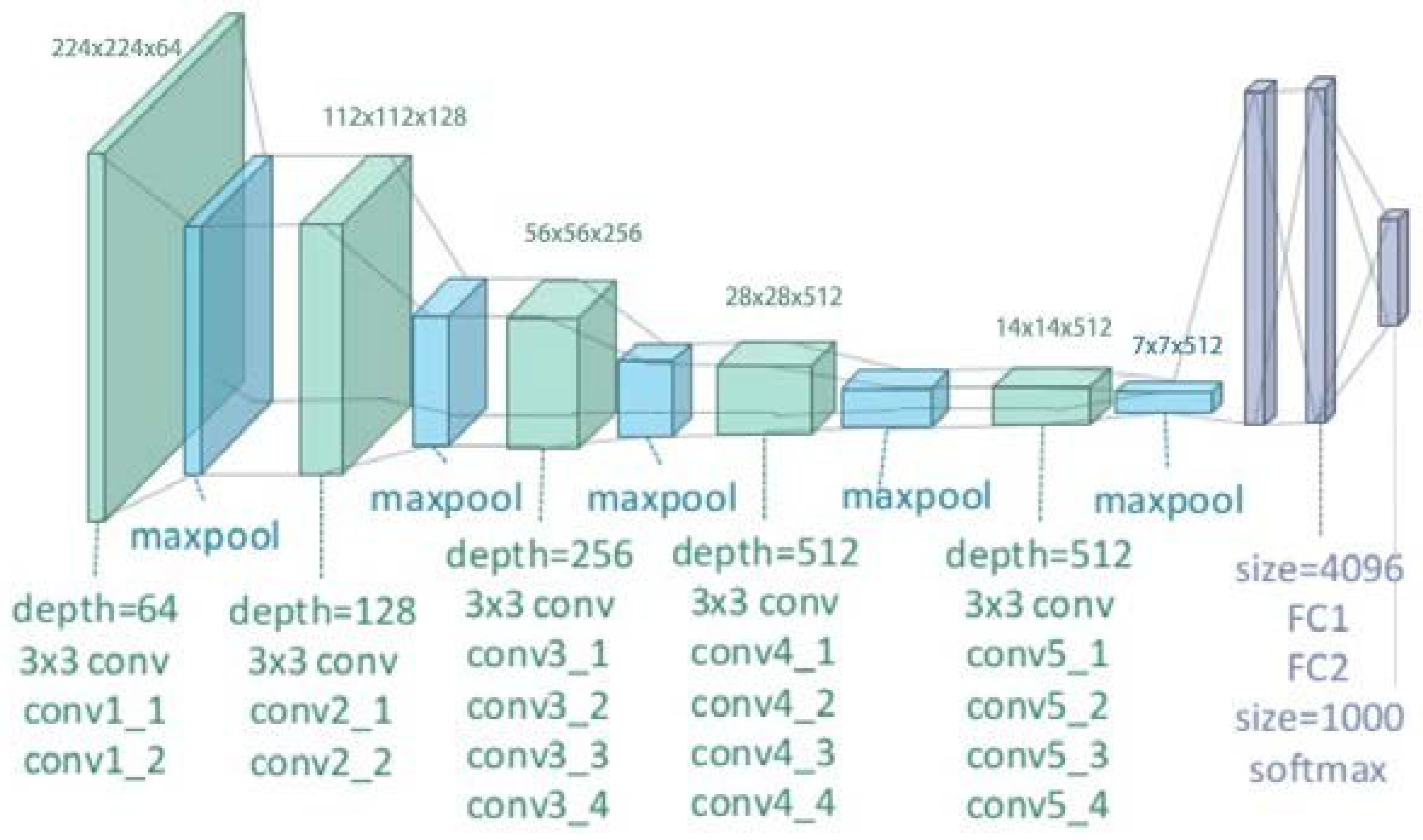
3.2.1. VGG-16
VGG-16 was developed by Visual Geometry Group (VGG) at the University of Oxford . It was introduced by Simonyan and Zisserman in 2014. VGG-16 became a benchmark in field of computer vision since it achieved an accuracy of 92.77% on ImageNet dataset which contains 14 million images and 1,000 different classes [82].
Vgg-16 consists of 16 weight layers and its structure consists of 13 convolutional layers organized into five blocks as shown in Figure 3 [83]. Each block has multiple convolutional layers and a max-pooling layer. Moreover, there are 4096 channels in first two layers, and 1000 channels in the third layer and represents 1000 different labels categories. The last layer is SoftMax activation function that outputs the probability distribution over classes typically used with 1000 output units for ImageNet classification and all hidden layers are followed by relu nonlinear activation function.
The input image that VGG-16 receives is typically 224 × 224 pixels with 3 color channels, RGB. When this input image goes through model’s first set of convolutional layers, then the number of channels increases from 3 to 64. Then, after it passes through a max-pooling layer, the input image’s width and height are reduced by half making it 112 × 112 pixels from 224 × 224 pixels, it will keep 64 channels though. This pattern continues as the input image moves through vgg-16’s network. The final set of convolutional layers produces an output of 7 × 7 pixels with 512 channels. After this, the output is passed through three fully connected layers which results in 1 × 1 × 1000, which means 1000 values. These 1000 values are then fed into the SoftMax activation function that normalizes them into a range between 0 and 1 (with all the values adding up to 1). This process helps determine the probability that the image belongs to each of the 1000 categories that VGG-16 can classify [85] .
3.2.2. VGG-19
VGG-19 is a convolutional neural network (CNN) architecture developed by the Visual Geometry Group (VGG) at the University of Oxford. VGG 19 architecture has 3 Fully connected layers, 16 convolution layers, 1 SoftMax layer, and 5 MaxPool layers [82]. Just like Vgg 16, Vgg-19 was also introduced in 2014 by Simonyan and Zisserma. VGG-19 features 19 weight layers, comprising 16 convolutional layers and 3 fully connected layers. The architecture is similar to VGG-16 but with increased depth, achieved by adding more convolutional layers to the last three blocks (see Figure 4). Each convolutional block in VGG-19 is followed by a max-pooling layer similar to vgg-16, which helps reduce the spatial dimensions, and the network ends with the same fully connected layers as VGG-16.
Since VGG-19 has additional layers which makes it more powerful as compared to VGG-16.Additional layers allows model to capture even finer details in data which improves its performance on complex visual tasks, such as object detection and image segmentation [86]. However, VGG-19 is computationally more expensive than VGG-16, with approximately 143 million parameters [87].
Figure 4.
Architecture of VGG-19 [88]
Figure 4.
Architecture of VGG-19 [88]
3.2.3. AlexNet
AlexNet was developed by Krizhevesky et al in 2012. It won ImageNet Large Scale Visual Recognition Challenge (ILSVRC) in 2012. Before AlexNet, CNN was limited to hand digit recognition tasks and AlexNet is recognized as the first model that revolutionized image classification and recognition [75].
Figure 5.
Architecture of AlexNet [89]
Figure 5.
Architecture of AlexNet [89]
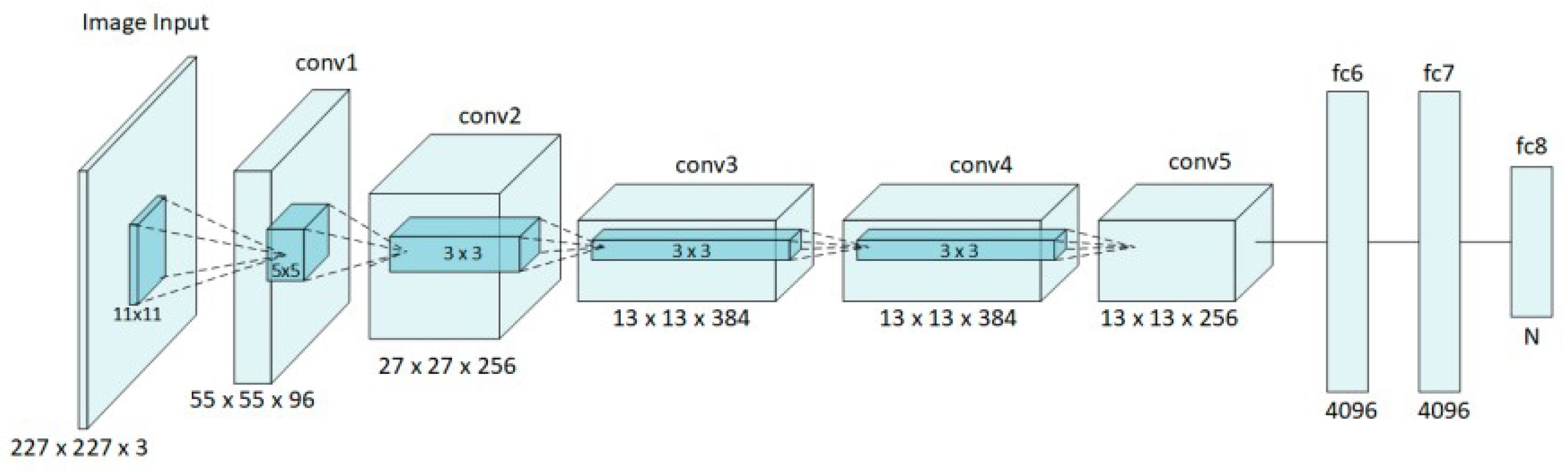
Moreover, AlexNet introduced several key innovations that contributed to its success. One of them was the use of the Rectified Linear Unit (ReLU) activation function that significantly sped up the training process and to prevent overfitting, Alexnet also employed dropout in the fully connected layers which randomly "drops" neurons during training to encourage the network to learn more robust features. Another innovation was the use of overlapping max-pooling which enhanced the richness of features and AlexNet also makes use of GPUs for computing acceleration [90].
The architecture of AlexNet has eight layers with five convolutional layers followed by three fully connected layers [91] (see Figure 5). The first convolutional layer uses 96 filters of size 11x11 with a stride of 4, applied to the input image, and is followed by a max-pooling layer. The second convolutional layer applies to 256 filters of size 5x5 and also includes max-pooling. The third, fourth, and fifth convolutional layers use 384, 384, and 256 filters, respectively, with only the fifth layer followed by max-pooling. These convolutional layers are designed to extract increasingly complex features from the input image, while the max-pooling layers reduce the spatial dimensions, helping to control the number of parameters and computational load. Additionally, there are 4096 neurons in each fully connected layer [91]. Following the convolutional layers, the output is flattened and passed through three fully connected layers. The final fully connected layer has 1000 neurons, corresponding to the 1000 classes in the ImageNet dataset and finally, the output of this last layer is processed through a softmax function to produce the class probabilities [92].
3.2.4. LeNet-5
LeNet-5 is one of the earliest Convolutional Neural Networks (CNNs) developed by Yann LeCun in 1998 [93]. It was specifically designed for handwritten digit recognition, such as the digits used in the MNIST dataset [94]. The architecture of LeNet-5 is relatively simple by modern standards and is very famous as it was the first CNN. LeNet-5 is a feed forward neural network and consists of seven layers with two convolutional layers, two pooling layers, and three fully connected layers [90] (as shown in Figure 6). The input to the network is a 32x32 grayscale image.
The first layer is a convolutional layer (C1) that consist of six 5x5 filters that produce six feature maps of size 28x28. This layer captures low-level features such as edges and simple shapes. Next layer is subsampling (S2) or average pooling layer that reduce dimensions of feature maps to 14x14 by uisng a 2x2 filter with a stride of 2. This step reduces computational complexity and ensures network is more invariant to small translations of input. Following this, another convolutional layer (C3) which has sixteen 5x5 filters is applied that generates sixteen 10x10 feature maps. Unlike first convolutional layer, this layer doesn’t connect every input map to every output map, instead it use specific pattern of connections that reduces the number of parameters and introduces some degree of specialization among feature maps.
The next layer is another subsampling (S4) layer, which further reduces the feature maps to 5x5. After this, a third convolutional layer (C5) with 120 5x5 filters is applied, but since the input size to this layer matches the filter size, the output is a set of 120 1x1 feature maps, effectively functioning as fully connected layers. The final layers include a fully connected layer (F6) with 84 neurons, which is connected to the output layer that has ten neurons—one for each digit class in the MNIST dataset. The activation function used throughout LeNet-5 is sigmoid or hyperbolic tangent (tanh) [93].
3.2.5. GoogleNet
Googlenet also known as Inception v1 and it was introduced by Google in 2014 [96]. The main goal was to achieve highest accuracy with less computational cost. Additionally, it won the ImageNet Large Scale Visual Recognition Challenge (ILSVRC) in 2014. The architecture of GoogLeNet is 22 layers deep (or 27 layers if pooling is included) [97]. Its innovative use of the Inception module, which allows the network to capture complex features at multiple scales with reduced computational cost [75] (see Figure 7).
The Inception module is main building block of GoogLeNet [98]. It was designed to address the issue of choosing optimal filter size at each layer. Instead of selecting single filter size, the Inception module applies multiple filters (1x1, 3x3, and 5x5) as well as a 3x3 max-pooling operation in parallel to input. Then the outputs from these operations are concatenated along depth dimension which results in rich feature representation that captures both local and global features at the same time. The 1x1 convolutions within the module serve two purposes i-e they help reduce the dimensionality of the data, thereby lowering the computational complexity, and they also enable network to learn more intricate patterns by combining multiple feature maps [97].
Figure 7.
Architecture of GoogleNet [99]
Figure 7.
Architecture of GoogleNet [99]
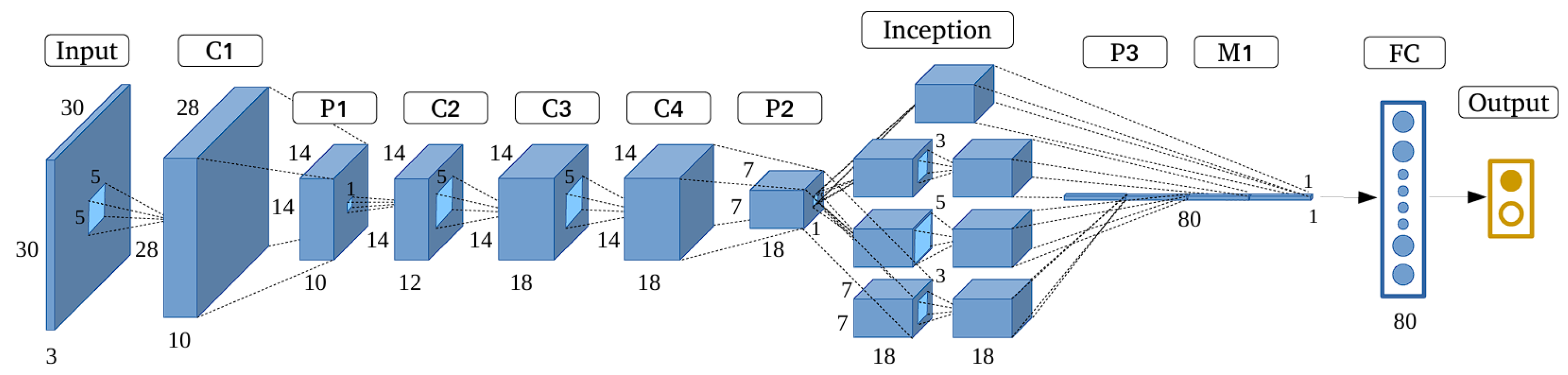
The overall architecture of GoogleNet begins with convolutional and max-pooling layers to process input, which is typically 224x224 pixels. The initial layers apply a 7x7 convolution followed by max-pooling, then a series of 1x1 and 3x3 convolutions to further refine feature maps. After these preliminary layers, the network transitions into main body, which consists of 9 stacked Inception modules. These modules are grouped into three sections each progressively increasing in complexity. This modular design allows network to capture increasingly abstract representations of the input as it moves deeper into the network.
To address vanishing gradient problem, GoogLeNet includes two auxiliary classifiers which are connected to intermediate layers [100]. These auxiliary classifiers act as additional sources of gradient flow during training which can help network converge more effectively.
Rather than using fully connected layers as we have seen in earlier CNN architectures, GoogLeNet use a global average pooling layer before the final output [101]. This layer averages spatial dimensions of feature maps which produce a compact 1x1 feature vector for each class, which is then fed into a softmax layer to generate final classification probabilities. This approach significantly reduces the number of parameters that make GoogLeNet more efficient in terms of both memory and computation. Moreover, GoogleNet has approximately 5 million parameters [102]. GoogLeNet show that deep networks can achieve high performance without being overly resource intensive.
3.3. ResNet
ResNet stands for Residual Network, was introduced by He et al in 2015 [103] . ResNet employed residual learning that can handle the vanishing gradient problem [104]. This problem occurs when gradients become too small during back-propagation which makes it difficult to update the weights effectively in very deep networks. In a traditional neural network, each layer learns a function that directly maps input to output. However, as networks grow deeper, it becomes difficult to optimize this mapping. ResNet addresses this by introducing residual blocks that allow each layer to learn the residual or difference between the input and the desired output, rather than directly learning the output [105]. This skip connection helps preserve the flow of gradients during backpropagation, making it feasible to train very deep networks without encountering the vanishing gradient problem.
Figure 8.
Architecture of ResNet [106]
Figure 8.
Architecture of ResNet [106]
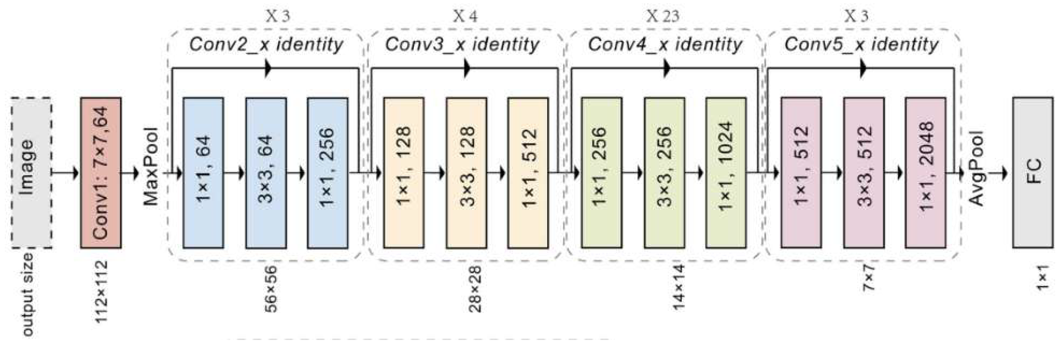
The architecture typically starts with a conventional convolutional layer, followed by a series of residual blocks grouped into stage where each stage is responsible for learning features at different levels of abstraction. In a residual block the input x is passed through two weight layers, each followed by a ReLU activation function, producing an output . This output is then added to the original input x .The combined result is then passed through another ReLU activation as shown in Figure 9 .
Residual block use skip connection. The identity shortcut directly pass input to output, while convolutional shortcut involves a 1x1 convolution operation. This approach allows ResNet to handle cases where input and output have different dimensions which ensures shortcut connections are valid. Additionally, ResNet blocks often include batch normalization and ReLU (Rectified Linear Unit) activation functions, which further stabilize training and improve the network’s ability to learn complex patterns (see Figure 8 ).
Another significant aspect of ResNet is its bottleneck design in deeper variants like ResNet-50, ResNet-101, and ResNet-152 [107]. In these architectures, each residual block contains three layers instead of standard two, i-e a 1x1 convolution layer that reduces the number of channels (dimensionality reduction), followed by a 3x3 convolution layer that processes the reduced representation, and finally another 1x1 convolution layer that restores the original number of channels. This bottleneck structure reduces computational load and memory usage.
At the end of network, ResNet typically use global average pooling layer, similar to GoogLeNet, to reduce the spatial dimensions of the final feature maps before feeding them into a fully connected layer that produces the output classification. The global average pooling layer helps to minimize number of parameters and avoid overfitting while also ensuring that network remains computationally efficient.
ResNet architectures come in various depths such as Resnet-50,101 and 152. However, Resnet-152, which has 152 layers, won the 2015-ILSVRC competition. The performance of ResNet in image recognition tasks highlights the crucial role of representational depth in a wide range of visual recognition tasks [75].
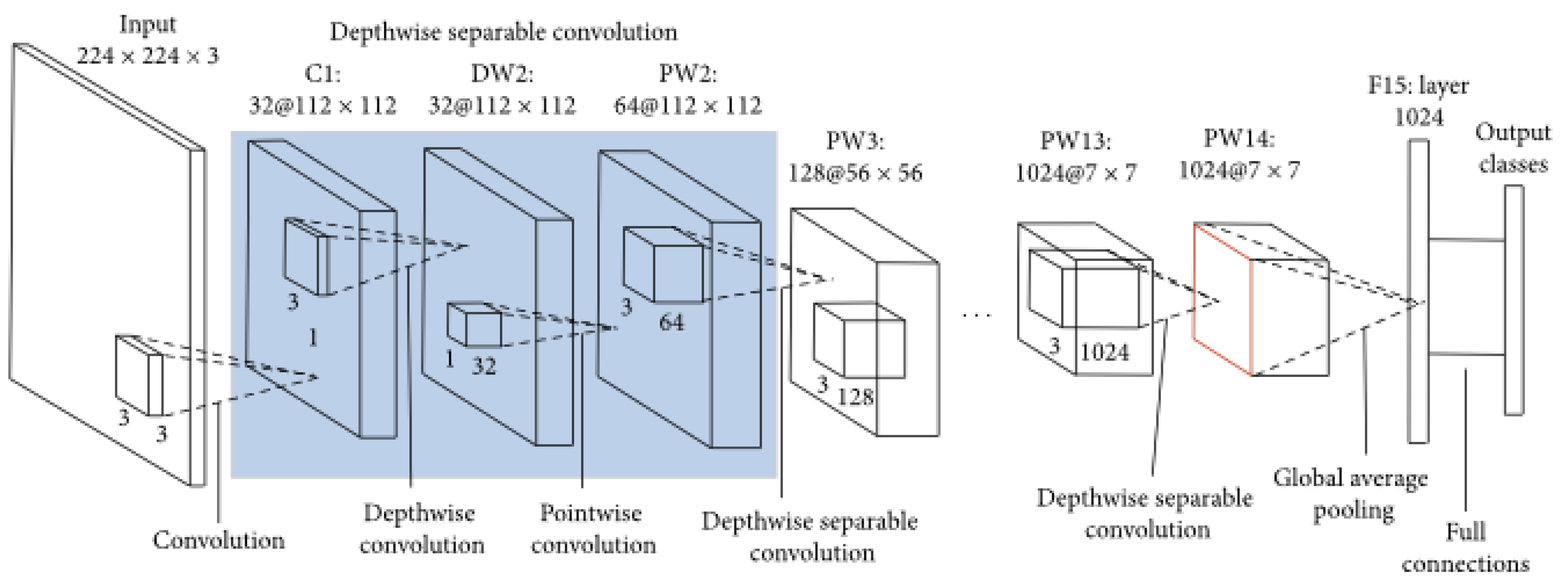
3.3.1. MobileNet
MobileNet’s main goal was to provide an efficient, lightweight model suitable for mobile and embedded devices, where computational resources are limited. Moreover, MobileNet introduces depth-wise separable convolutions ,= a technique that can reduce number of parameters and computational complexity which make it good for environments with restricted computational power [108].
In a standard convolutional layer, each filter is applied to all input channels, and then the results are combined to produce the output feature map. This process is computationally expensive, especially as the number of filters and input channels increases. MobileNet addresses this inefficiency by breaking the standard convolution operation into two simpler and more efficient operations, i-e depthwise convolution and pointwise convolution [109]. In depthwise convolution, a single convolutional filter is applied independently to each input channel, rather than across all channels. This step reduces the number of computations significantly because each filter only needs to process one channel at a time. Architecture of Mobilenet is shown in Figure 10.
Following the depthwise convolution, MobileNet uses a pointwise convolution, which is essentially a 1x1 convolution applied across all channels [108]. The pointwise convolution combines the outputs from the depthwise convolution and allows the network to mix the information across channels. By separating the spatial and channel-wise operations, MobileNet dramatically cuts down the number of parameters and floating-point operations (FLOPs) required, without a significant loss in accuracy.
The original MobileNet architecture, often referred to as MobileNetV1, is composed of a series of these depthwise separable convolutions, organized in blocks that allow the network to learn increasingly complex features at each layer. MobileNetV1 also introduces a couple of hyperparameters i-e width multiplier and resolution multiplier that allow users to tradeoff between model size, speed, and accuracy [110]. The width multiplier reduces the number of channels in each layer, effectively thinning the network, while the resolution multiplier reduces the input image size, making the model faster and lighter at the expense of some accuracy.
Figure 10.
Architecture of MobileNet [111]
Figure 10.
Architecture of MobileNet [111]
Building on the success of MobileNetV1, MobileNetV2 introduced several enhancements, including the inverted residual block with linear bottlenecks. The inverted residual block begins with a pointwise convolution to expand the number of channels, then applies a depthwise convolution, and finally uses another pointwise convolution to reduce the number of channels back to the original count . The use of linear bottlenecks at the end of these blocks prevents the loss of information during dimensionality reduction, which can occur with non-linear activations like ReLU . This structure maintains efficiency and improves the performance of the model.
MobileNetV3 further refines the architecture by incorporating advances like the swish activation function and squeeze-and-excitation (SE) modules. These SE modules adaptively recalibrate the channel-wise feature responses, enhancing the representational power of the network. MobileNetV3 use NAS (Neural Architecture Search) to automatically discover and optimize the model architecture, striking a better balance between latency and accuracy across a range of mobile devices [90].
3.3.2. Xception
Xception stands for “Extreme Inception” is a deep Convolutional Neural Network (CNN) architecture proposed by François Chollet in 2017 as an extension and improvement of the Inception model family. The core idea behind Xception is to replace the Inception modules with depthwise separable convolutions [75]. Depthwise separable convolutions significantly enhances both the computational efficiency and the representational power of the network.
Figure 11.
Architecture of Xception [112]
Figure 11.
Architecture of Xception [112]
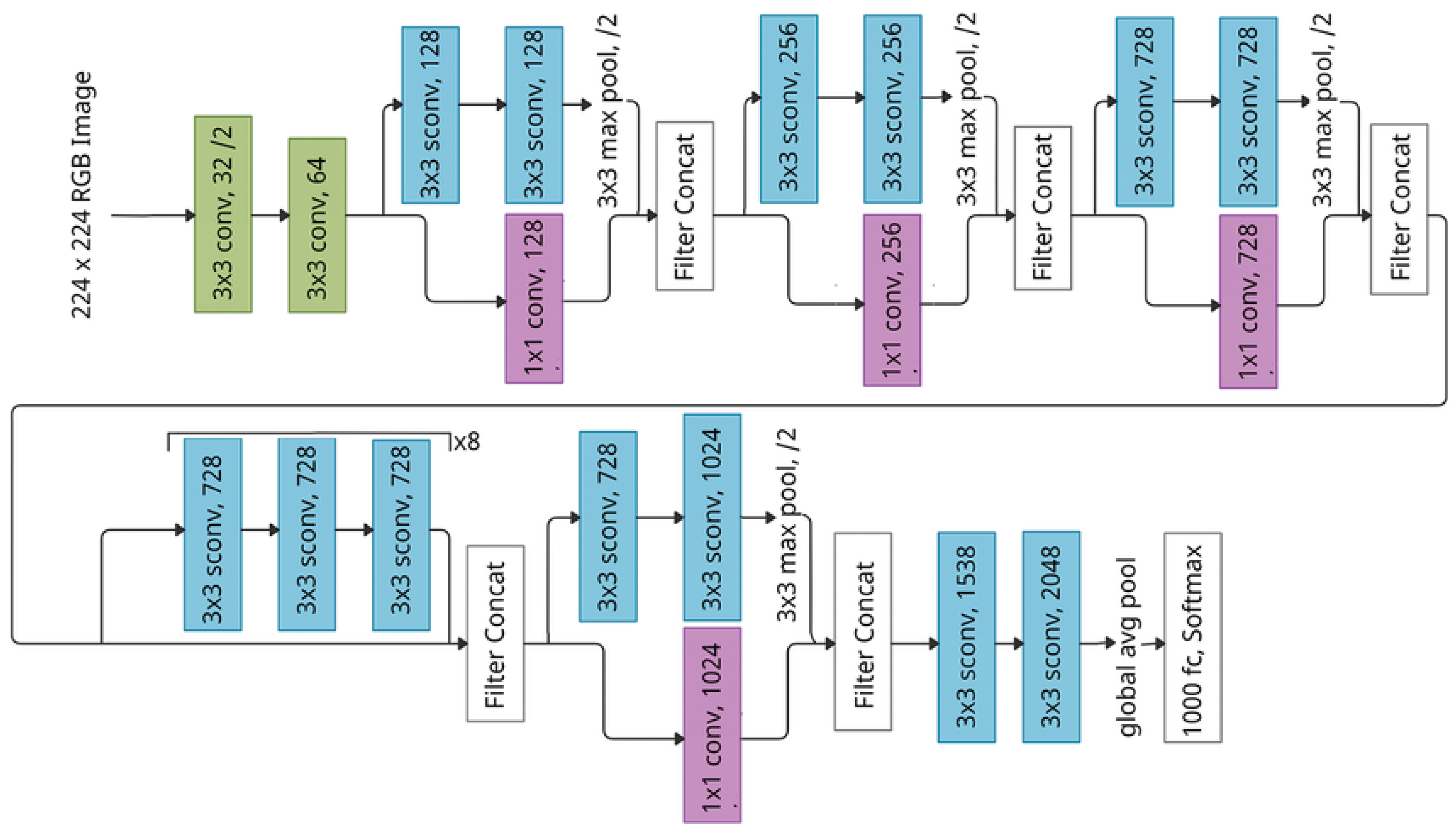
The architecture of Xception is based on principle of depthwise separable convolutions which decompose standard convolution operation into two separate steps i-e depthwise convolution and pointwise convolution [113] . In a depthwise convolution, a single filter is applied to each input channel independently, rather than applying multiple filters across all channels simultaneously. This step captures spatial relationships within each channel without mixing channels. Following this, a pointwise convolution (a 1x1 convolution) is applied across all channels to combine the features learned in the depthwise step [75]. This separation of spatial and cross-channel convolutions reduces the computational complexity significantly while allowing the network to learn more nuanced and fine-grained features.
The Xception architecture consists of 36 convolutional layers organized into 14 modules, with each module containing one or more depthwise separable convolution layers [114] (see Figure 11).
Xception uses residual connections inspired by the ResNet architecture [101]. In Xception, residual connections are employed across most modules to allow for more efficient gradient flow and to mitigate the vanishing gradient problem. These connections help the network maintain high accuracy even as the number of layers increases, enabling the training of deeper networks without significant degradation in performance.
In the final stages of the architecture, Xception employs global average pooling instead of fully connected layers [115]. This layer averages each feature map into a single value which drastically reduces the number of parameters and prevents overfitting. The output from this layer is then fed into a softmax classifier to produce the final predictions.
3.3.3. DenseNet
DenseNet stands for Dense Convolutional Network and was introduced by Gao, et al. in 2017 Ṫhe main idea behind DenseNet is its unique connectivity pattern where each layer is directly connected to every other layer in a feed-forward manner to improve information flow between layers . In a DenseNet, each layer receives inputs from all preceding layers and passes on its output to all subsequent layers [116] (as shown in Figure 12). This is achieved by concatenating feature maps from previous layers, rather than summing them up as done in traditional residual networks like ResNet. As a result, the input to any given layer includes not only the raw input data but also feature maps from all of the preceding layers that provide network with a rich set of features at each stage . This dense connectivity allows more efficient flow of information and gradients throughout network.
The structure of DenseNet is organized into blocks known as Dense Blocks. Within each dense block, every layer is connected to every other layer that forms a highly interconnected network. Between these dense blocks, transition layers are used to control complexity of model by reducing the size of the feature maps through a combination of convolution and pooling operations .
DenseNet has better parameter efficiency as compared to Resnet . Despite the dense connections, DenseNet requires fewer parameters. For instance, there are 15.3 M parameters in 250-layer Densenet model. DenseNet also benefits from improved feature reuse because of input concatenation, the feature-maps learned by any of the DenseNet layers is accessible to all subsequent layers [116].
DenseNet is available in several variants, such as DenseNet-121, DenseNet-169, DenseNet-201, and DenseNet-264, which differ primarily in the number of layers and the depth of the dense blocks.
3.3.4. EfficientNet
EfficientNet is introduced by Google in 2019 [118]. It is designed to achieve state-of-the-art performance on image classification tasks while being more computationally efficient than previous architectures [119]. The key innovation behind EfficientNet is the development of a compound scaling method to balance the depth, width, and resolution of model systematically and efficiently [120]. This approach allows EfficientNet to scale up the model to achieve higher accuracy while maintaining a lower computational cost compared to traditional methods that scale only one dimension at a time, such as depth or width alone.
EfficientNet begins with EfficientNet-B0 that is a relatively small and simple model trained using techniques like neural architecture search (NAS) which is a technique for automating the design of neural network [118]. The real power of EfficientNet comes from its scaling strategy. The authors of EfficientNet introduced a compound scaling method that uniformly scales all dimensions of the network including depth (the number of layers), width (the number of channels in each layer), and resolution (the input image size) [121]. Compound scaling applies a carefully balanced scaling factor to all three dimensions simultaneously, ensuring that the network grows in a balanced and optimized way. This method allows EfficientNet to maintain high accuracy while using significantly fewer parameters and FLOPs (floating point operations) than previous state-of-the-art models. Furthermore, it utilizes Squeeze-and-Excitation Networks that improve channel interdependencies [118]. Architecture of EfficientNet is shown in Figure 13 .
The architecture of EfficientNet is built upon MobileNetV2’s inverted residual blocks [118]. These blocks consist of an expansion phase, a depthwise convolution, and a projection phase, which helps the network learn more complex features without a significant increase in computational cost.
EfficientNet-B0, the smallest model in the EfficientNet family, starts with a 224x224 input image size and uses these inverted residual blocks throughout its architecture. As you move up the EfficientNet family from B0 to B7, the models become progressively larger, and use higher input resolutions, more channels, and deeper networks, all according to the compound scaling formula. One of the most impressive features of EfficientNet is its scalability across a wide range of model sizes. The smallest model, EfficientNet-B0, has only 5.3 million parameters [123].
3.4. Evaluation Metrics
Evaluation metrics give a quantitative mean to see how well a model performs [124]. They also help with comparison of different models to determine the most effective one for a certain task. Additionally, evaluation metrics are derived from confusion matrix [125]. Confusion matrix summarizes the performance of a model by comparing predicted labels to actual labels. The key components of confusion matrix are True Positives (TP), True Negatives (TN), False Positives (FP), and False Negatives (FN) . We have discussed all of these in details below.
True Positive: True positive is when both prediction and actual values are correct or we can say when the model’s prediction matches the actual values . For instance, correctly identifying a malignant case as malignant.
True Negative: When both prediction and actual values are same such as correctly identifying a benign case as benign, it is considered a true negative.
False Positive: False positive is when a model prediction is yes but actual value is no such as model predicts a benign caseas malignant (Type I error).
False Negative: False positive is when a model prediction is no but actual value is yes such as model predicts a malignant case as benign (Type II error) [126].
The key performance metrics that we used to evaluate CNN architectures are discussed below. It includes Accuracy, Precision, Recall, Specificity, F1-Score, False Positive Rate (FPR), False Negative Rate (FNR), False Discovery Rate (FDR), Area Under the Curve (AUC), and Time Complexity.
3.4.1. Accuracy
Accuracy measures overall correctness of model. It is calculated as number of all correct predictions (both benign and malignant) divided by total number of the dataset . Accuracy is given by equation [126]:
Where,
TP is True Positive, FP is False Positive, FN is False Negative, and TN is True Negative.
3.4.2. Precision
Precision focuse on quality of positive predictions (malignant cases). It answers the question, "Out of all predicted malignant cases, how many were actually malignant?". It is calculated as amount of True positive divided by predicted. It is given by the equation [126]:
Where,
TP is True Positive and FP is False Positive.
3.4.3. Recall (Sensitivity or True Positive Rate)
Recall measures the ability of model to identify all actual malignant cases. It answers “Out of all actual malignant cases, how many did the model correctly predict?". It is calculated as an amount of True positive divided by actual yes . It is given by the equation [126]:
Where,
TP is True Positive and FN is False Negative.
3.4.4. Specificity
Specificity is how correctly model predicts the benign cases (true negative rate) . It answers the question, "Out of all actual benign cases, how many were correctly identified?". It is given by the equation [127]:
Where,
FP is False Positive and TN is True Negative.
3.4.5. F1-Score
The F1-Score is the harmonic mean of precision and recall. It is a balance between precision and recall. F1-Score is very useful when we have uneven class distribution. It is given by the equation [128]:
or
Where,
TP is True Positive, FP is False Positive, FN is False Negative, and TN is True Negative.
3.4.6. False Positive Rate (FPR)
FPR measures the proportion of benign cases that were incorrectly classified as malignant. It is also known as probability of a Type I error and is important in understanding the model’s performance in distinguishing between benign and malignant cases. FPR can be calculated by the equation [129]:
Where,
FP is False Positive and TN is True Negative.
3.4.7. False Negative Rate (FNR)
FNR represents the proportion of malignant cases that were incorrectly classified as benign, also called probability of Type II error [130]. FNR is given by the equation [129]:
Where,
TP is True Positive and FN is False Negative.
3.4.8. False discovery Rate (FDR)
FDR measures the proportion of incorrect predictions such as malignant cases that were actually benign [131]. A high FDR indicates that the model has a high number of false positives. FDR is given as [132]:
Where,
TP is True Positive and FP is False Positive.
3.4.9. Area under the curve (AUC)
3.5. Time Complexity
Time complexity specifically refers to the amount of computational time an algorithm takes to complete as the size of the input data grows. It is often expressed using Big O notation (e.g., O(n), O(log n)). Moreover, it is an important factor in determining efficiency of machine learning models.
Time Complexity of CNN is given by the equation [135]:
Where,
D is number of convolution layers of the neural network
i is the ith convolution layer of the neural network
M denotes the side length of the output characteristic graph of each convolution kernel
K is side length of each convolution kernel
is output channel of the ith convolution layer of the neural network.
Time complexity of VGG-16 is given by the equation [136]:
Where,
D is number of all convolutional layers of neural network
l is first convolutional layer of the neural network
is number of output channels of the lth convolutional layer
is number of fully connected layers
is number of features to be output in that layer.
Time complexity of VGG-19 is given by the equation [137]:
Where,
l is subscript of convolutional layer
d is number of convolutional layers
is number of convolution kernels in the lth network
is number of input channels in the lth network
is size of a convolution kernel
is the size of the output feature map.
Time complexity of AlexNet is given by the equation [138]:
Where,
n represents number of convolutional layers
is number of input channels of the jth layer
is number of filters of the jth layer
is spatial size of the filters
denotes size of output feature map.
Time complexity of Mobilenet-v2 is given by the equation [139]:
Where,
L is number of layers and M is number of output feature maps in each layer
N is number of input feature maps in each layer
is the number of operations performed.
The total number of operations is given by the following equation:
Where,
D is the number of images in the dataset. The computational complexity is given by the following equation:
Where,
F is the number of floating-point operations per second.
Time complexity of Xception is given by the equation [135]:
Where,
D is number of convolution layers of the neural network
i is the ith convolution layer of the neural network
Mdenotes the side length of the output characteristic graph of each convolution kernel
K is the side length of each convolution kernel
represents the output channel of the ith convolution layer of the neural network.
Time complexity of ResNet is given by the equation [140]:
Where,
is the number of target symbols.
L represents the number of convolution layers in the i-th residual block (res-block).
is a characteristic of the convolution layer (e.g., kernel size).
and denote the input and output sizes of the l-th layer in the residual block.
refers to the output characteristic at the l-th layer (e.g., height or dimensionality of the output).
Time complexity of GoogleNet is given by the equation [141]:
Computational complexity can be given by Floating Point Operations Per Second (FLOPs). FLOPs indicates how many floating-point calculations a system can perform per second.
Time complexity of EfficientNet is given by the equation: FLOPs(Floating Point Operations Per Second) of EfficientNet are only 22.34 Million [142].
Time complexity of DenseNet is given by the equation [143]:
Where,
is input feature map channel
be dimensions of output feature map
T is map temporal dimension stacking
D is convolutional kernel size .
Time complexity of Lenet-5 is given by the equation [144]:
Where,
is the number of transmit antennas at the transmitter
is the number of receive antennas at the receiver.
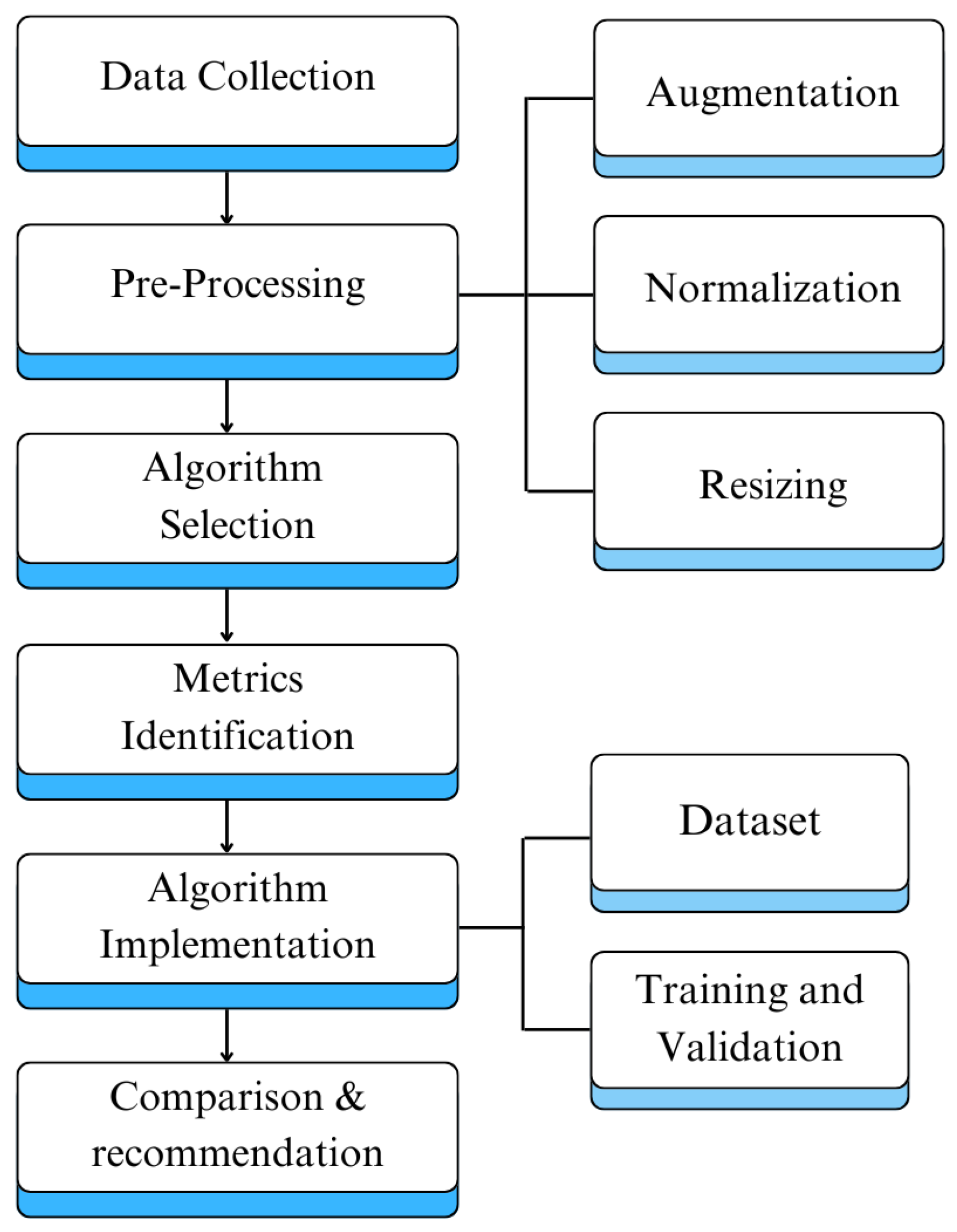
4. Methodology
The following methodology outlines systematic approach used to conduct this research. It involves data collection, image preprocessing, algorithm selection, algorithm implementation, performance evaluation, and providing recommendations based on our findings. We started our research with a comprehensive literature review to explore state-of-the-art. Moreover, we selected commonly used algorithms, datasets, and evaluation metrics. Then we implemented selected algorithms and assessed their performance on the basis of key performance metrics. Lastly, we provided comparative analysis and highlighted the trade-offs between various performance metrics.
Firstly, we conducted an in-depth literature review to identify commonly used datasets for skin cancer detection and classification. The most commonly used datasets in state-of-the-art are HAM10000, the dataset from ISIC archive, and PH2 [18]. We’ve summarized these datasets in Table 3.
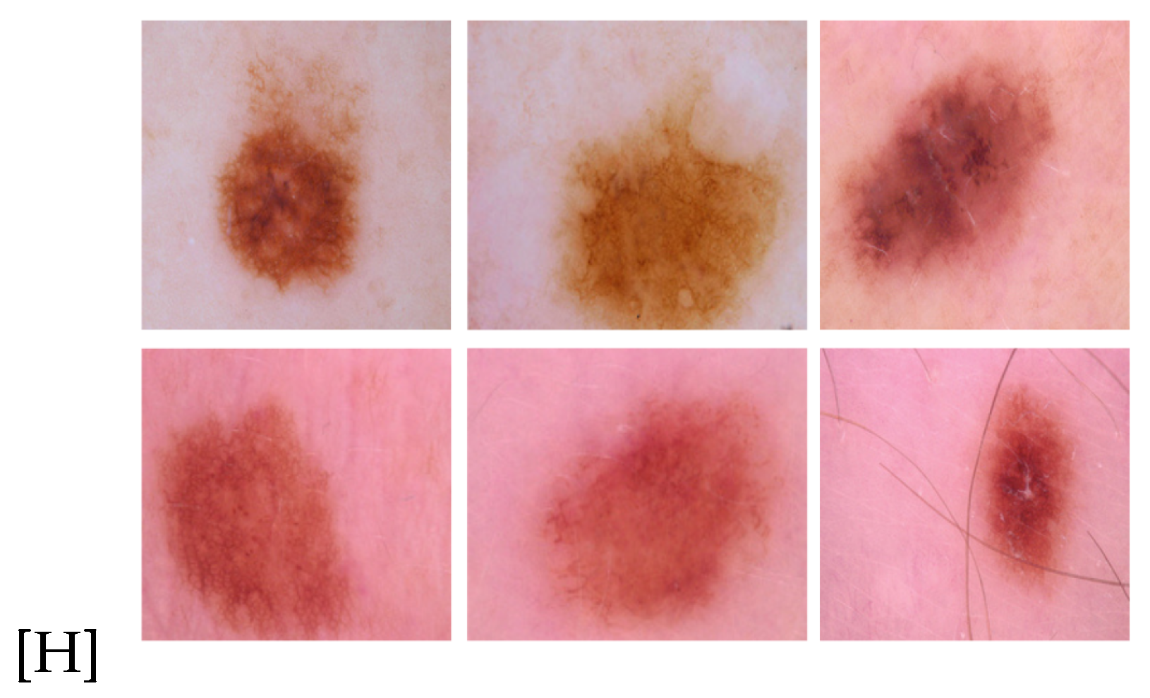
Figure 14.
Benign and Malignant images from ISIC archive
HAM10000. The HAM10000 (Human Against Machine) dataset is one of the largest and most used datasets for skin lesions classification [145]. It contains 11,720 images and sourced from International Skin Imaging Collaboration (ISIC) archive . Additionally, it’s created to facilitate training of machine learning and deep learning models in diagnosing skin cancer. This dataset include seven different classes of skin lesions which are Actinic Keratosis, Basal Cell Carcinoma , Benign Keratosis , Dermatofibroma , Melanoma , Melanocytic nevus and Vascular lesion [146]. The dataset is publicly available through the ISIC (International Skin Imaging Collaboration) Archive.
ISIC-2017. The ISIC 2017 dataset was developed for 2017 ISIC Challenge. It was developed for image analysis tools that can automatically diagnose melanoma from skin lesions [147]. ISIC 2017 dataset consists of 2750 skin cancer images with 2000 images for training datasets, 150 images for test datasets, and 600 images for validation datasets . Additionally, the size range for ISIC-2017 is 540 × 722 × 3 to 4499 × 6748 × 3 pixels [148].
ISIC-2018. The ISIC 2018 dataset was developed for 2018 ISIC Challenge. This dataset has more images as compared to ISIC 2017 dataset. It consists of 11527 images with 10,015 images for training and 1512 images for testing dataset. Moreover, ISIC 2018 consists of 7 different classes of skin lesions including Melanoma (MEL), Nevi (NV), Basal cell carcinoma (BCC), Actinic keratosis / Bowens disease (intraepithelial carcinoma) (AKIEC), Benign keratosis (BKL), Der- matofibroma (DF) and Vascular (VASC) [149].
PH2. The PH2 dataset is significantly smaller compared to other datasets listed above. It is collected from the Hospital Pedro Hispano in Portugal and it consists of only 200 images. Each image has a size of 768 × 560 pixels . It has 3 different types of skin lesions including Atypical Nevus, Common Nevus and Melanoma . Additionally, it includes 80 images of atypical nevi, 80 images of common nevi, and 40 images of melanoma cases [150].
For this study, we used a dataset from Kaggle, which is from ISIC archive. It consists of 3297 skin lesion images with a resolution of 224 × 224 pixels. Additionally, the dataset consists of two classes i-e benign and malignant. The benign class has 1440 training images and 360 testing images while the malignant class has 1197 training images and 300 testing images.

Table 4.
Dataset
| Benign | Malignant | |
|---|---|---|
| Training Dataset | 1440 | 1197 |
| Testing Dataset | 360 | 300 |
| Total | 1800 | 1497 |
The image preprocessing stage consist of several steps to ensure dataset is ready for model’s training:
Resizing. Dataset is resized to uniform dimensions. It ensures consistency across the dataset. Moreover, it is useful to meet the input requirements of various CNN architectures.
Normalization. Pixel values will be normalized to a standard range (e.g., 0-1). It improves the convergence of the neural networks during training.
Augmentation. Data augmentation techniques such as rotation, flipping, and zooming are applied to increase diversity of training set. It helps prevent overfitting. Moreover, data augmentation enhances the model’s generalization by exposing it to various transformations of images.
The commonly used CNN architectures for skin cancer detection and classification were selected. The selected algorithms for our study include DenseNet, AlexNet, VGG-16, VGG-19, MobileNet, Xception, EfficientNet, LeNet-5, ResNet and GoogLeNet. These models are chosen for their proven track record in image classification tasks.
The selected algorithms were implemented in Python with TensorFlow and Keras libraries. We used Google Collab for the implementation of the selected algorithms. Goggle Collab is a cloud-based platform that provides free access to GPUs which accelerates the training process. The results of implemented algorithms are given in Table 5 and Table 6.
Additionally, we conducted an in-depth literature review to find the key performance metrics used to assess performance of algorithms in medical image analysis. The most commonly used metrics include accuracy, precision, recall, F1-score and specificity [7] - [18]. In addition to this, Specificity, False Positive Rate (FPR), False Negative Rate (FNR), False Discovery Rate (FDR), Area Under the Curve (AUC), and Time Complexity are also used in literature to evaluate the performance of algorithms. Therefore, we used these key performance metrics to assess the performance of selected algorithms.
After implementing the selected algorithms their performance is evaluated based on identified metrics. Furthermore, a detailed comparative analysis of implemented algorithms based on identified key metrics is provided.
Figure 15.
Proposed Approach Schematic
5. Results & Discussion
A detailed comparison of Convolutional Neural Network (CNN) architectures that we have implemented is given below. The Table 5 and Table 6 show the performance of these architectures across several key metrics that include accuracy, precision, recall, F1-score, specificity, False Positive Rate (FPR), False Negative Rate (FNR), False Discovery Rate (FDR), and the Area Under the Curve (AUC).
Figure 16.
Accuracy of CNN models
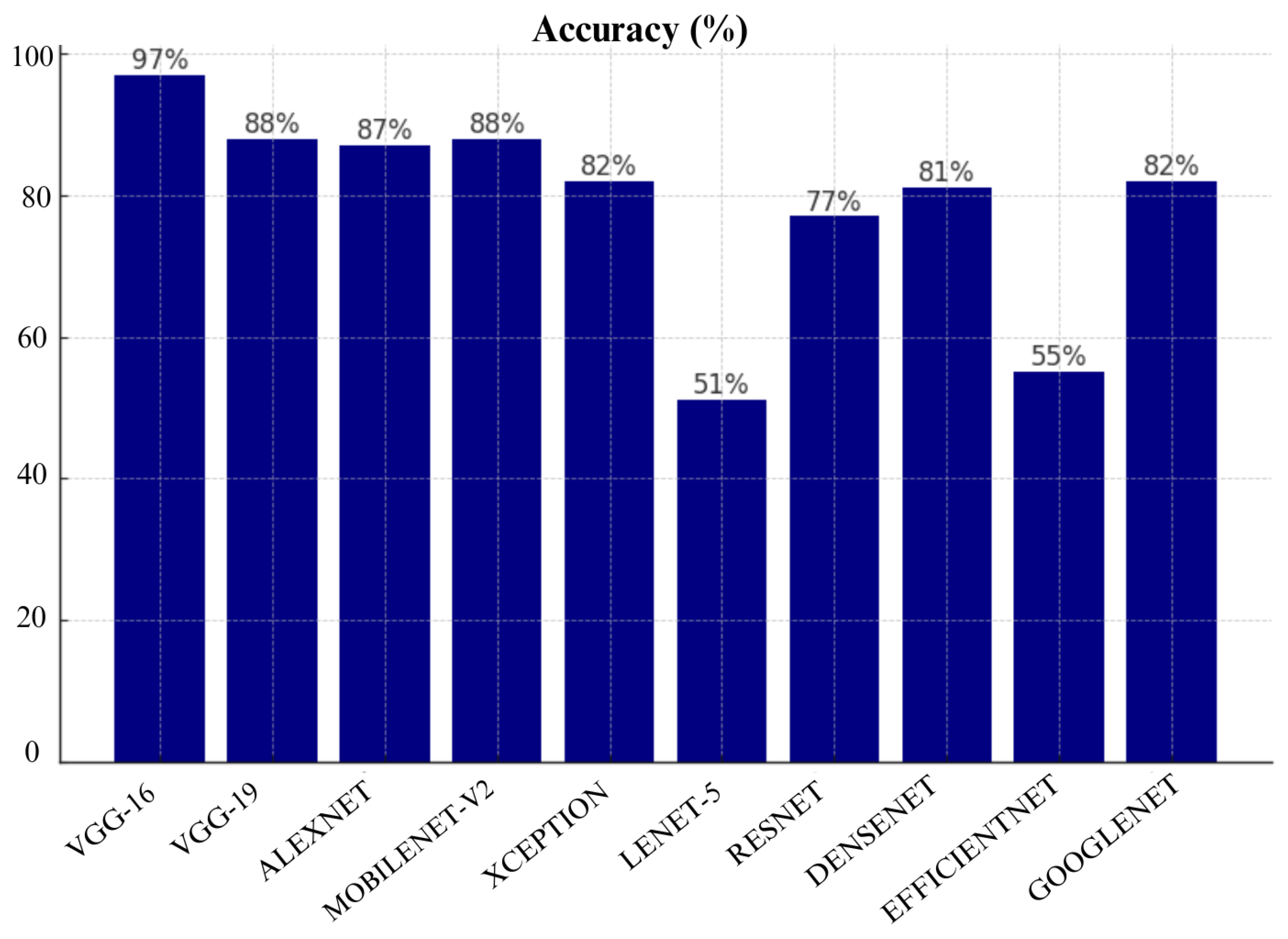
VGG-16 achieved highest accuracy of 97%, followed by VGG-19 with 88%, and MobileNet-V2 with 88% as shown in Table 16. These results show that VGG-16 is the most reliable in terms of making correct predictions. Other CNN architrectures such as GoogLeNet and Xception also performed well with an accuracy of 82%. However, models like Lenet-5 and EfficientNet show poor performance as they achieved accuracy of only 51% and 55%, respectively.
As shown in Figure 17, MobileNet-V2 achieved highest precision of 88%, closely followed by VGG-16, VGG-19 and Alexnet. VGG-16, VGG-19 and Alexnet performed equally well by achieving precision of 87%. These models show consistent precision which indicates that they can be trusted to avoid false positives. However, EfficientNet had a precision score of only 27% which shows that it is highly unreliable. Lenet-5 also performed poorly as it achieved precision of only 50%.
As shown in Figure 18, VGG-16 again had the best recall score of 87%, followed closely by MobileNet-V2 and VGG-19 with recall of 88% and 87% respectively. GoogLeNet and Xception also performed well with 82% recall each. However, Lenet-5 and EfficientNet performed poorly as they achieve only 50% recall which indicates that they have failed to detect a huge portion of malignant cases which may result in missed diagnoses in real-world applications.
Furthermore, MobileNet-V2 stands out with highest F1-score of 88% as you can see in Figure 19. It shows MobileNet-V2’s balanced performance in both precision and recall. VGG-16 and VGG-19 follow closely, both have achieved an F1-score of 87% each. EfficientNet with its F1-score of just 35% show poor performance as compared to other architectures. It also shows that it does not perform well in both precision and recall. Lenet-5 also performed poorly here with only 50%.
As you can see Figure 20, Densenet has achieved specificity of 90%, followed by VGG-19 at 88%, and VGG-16 at 87%. This shows that these algorithms excel in correctly identifying benign cases. Lenet-5 performed the worst, with a specificity score of 63% which means that it frequently misclassified benign cases as malignant cases.
Densenet perfromed well by achieving FPR score of 10% as shown in Figure 21. Followed by VGG-19 and VGG-16 with False Positive Rate of 12% and 13%, respectively. These models performed well in minimizing false positives. Additionally, EfficientNet had the lowest FPR of 0%, but we have to be careful when considering this result since the model’s overall performance was not good in other metrics. On the other hand, Lenet-5 had the highest FPR at 37% which means a very high chance of misclassifying benign cases and could lead to overdiagnosis.
As you can see in Figure 22, AlexNet and MobileNetv2 both performed very well and achieved a low FNR of 10% each. Closely followed by VGG-16, VGG-19 and ResNet with an FNR of 13% each. This shows they can be a good choice for effectively identifying malignant cases. On the other hand, EfficientNet and Lenet-5 achieved highest FNR of 100% and 64%, respectively. This makes EfficientNet and Lenet-5 a poor choice for skin cancer detection.
As shown in Figure 23, MobileNetv2 again performed well with FDR of only 10%, closely followed by VGG-19 which achieved False Discovery Rate (FDR) of 14%. These models show robustness in minimizing false discoveries. Additionally, EfficientNet had the lowest FDR of 0%, but we have to be careful when considering this result since the model’s overall performance was not good in other metrics. Moreover, Lenet-5 had a high FDR of 55% which further shows its unreliability in this study.
As shown in Figure 24, both VGG-19 and MobileNet-v2 achieved highest AUC scores of 88%. Followed by VGG-16 and AlexNet with an AUC of 87%. These models demonstrate a strong ability to distinguish between malignant and benign cases which makes them highly reliable. On the other hand, EfficientNet and Lenet-5 had the lowest AUC of 50% which further shows their unreliability.
Figure 24.
AUC of CNN models
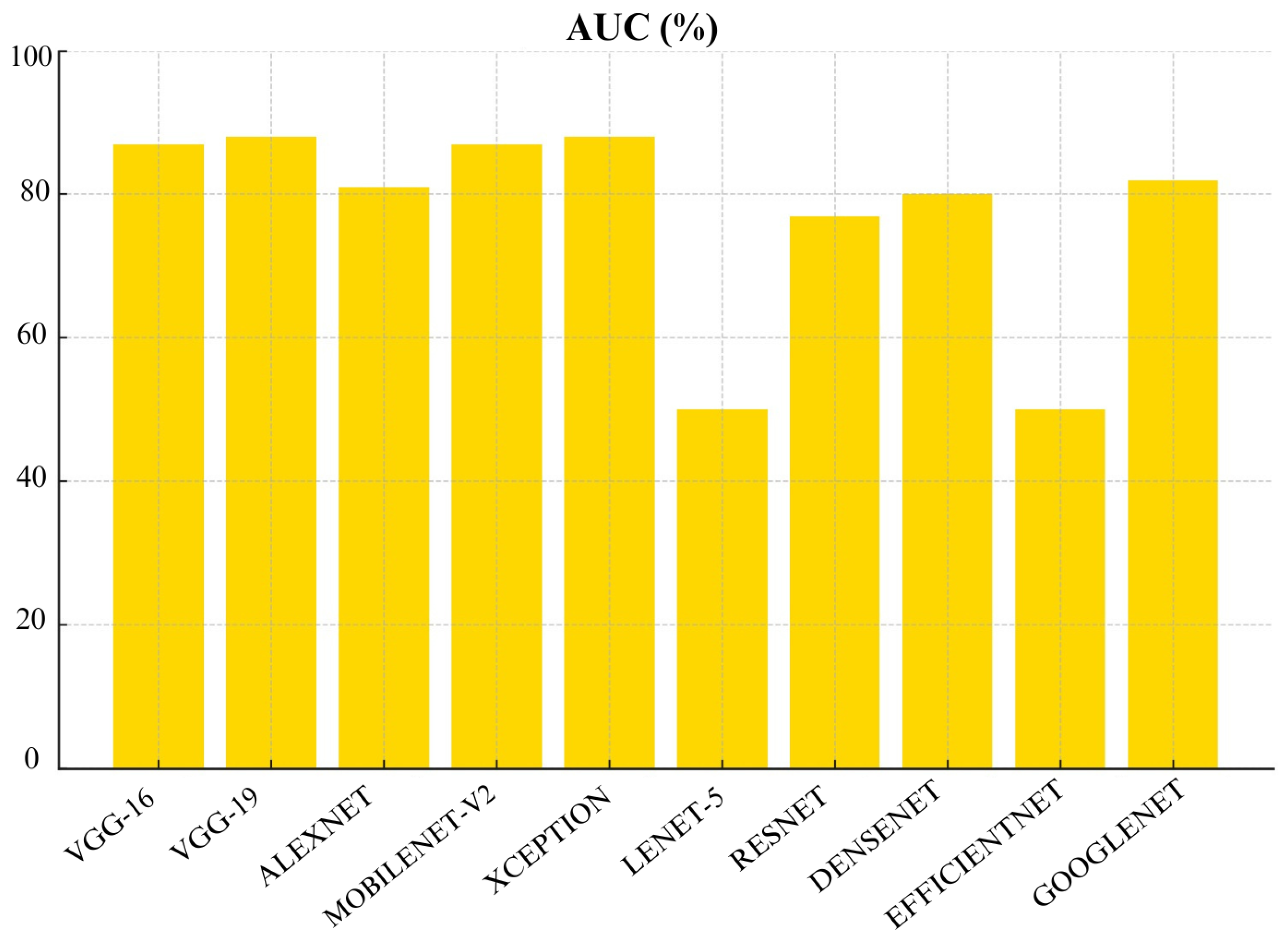
Figure 25.
Comparison of CNN models based on performance metrics
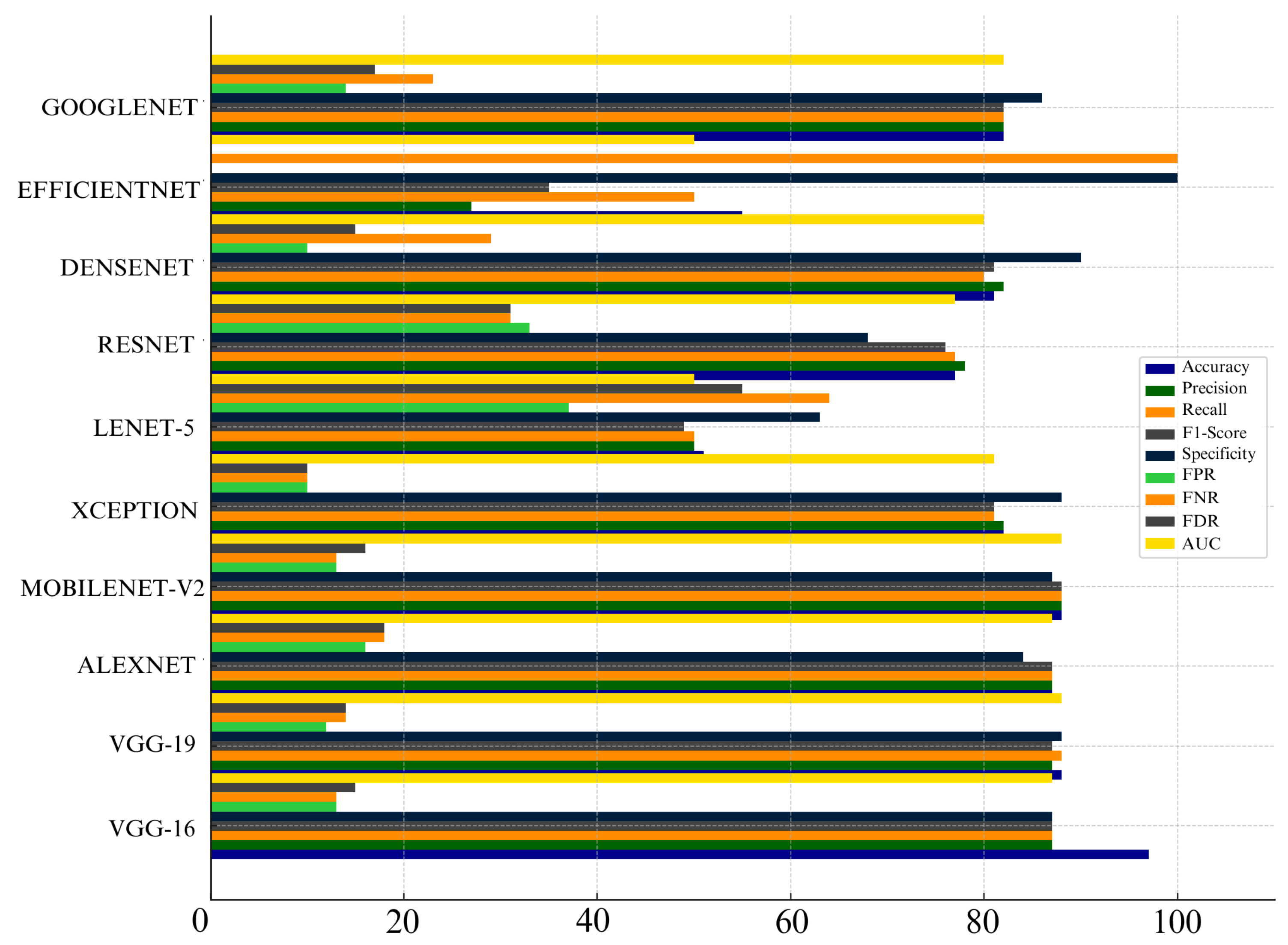
When we look at overall performance of algorithms across all metrics, we can see that certain CNN architectures perform well in specific metric. For instance, VGG-16 performed well in terms of accuracy, Precision, recall, and F1-score. VGG-19 also performed well in terms of precision and AUC. This means it’s good at distinguishing benign and malignant cases without too many false positives.
MobileNet-V2 also performed well across many metrics which include Precision, Recall, F1- score, FNR, FDR, and AUC. This make MobileNet-V2 a reliable choice for skin cancer detection and classification. Additionally, Densenet achieved lowest False Positive Rate (FPR) and False Discovery Rate (FDR) which make it highly reliable for avoiding unnecessary treatments. Meanwhile, Lenet-5 consistently struggled across almost all metrics which shows that it is not suitable for skin cancer detection and classification. Overall, choice of algorithm really depends on specific context and priorities in a medical setting. It depends whether you prioritize avoiding missed diagnoses (recall) or reducing false positives (specificity).
6. Conclusions
Based on our evaluation, we can conclude that MobileNetv2, VGG-16 and VGG-19 were top-performing CNN architectures in this study. MobileNetv2 performed well across many metrics which include Precision, Recall, F1- score, FNR, FDR, and AUC. It achieved the highest Precision, Recall, F1- score and AUC scores of 88% each. VGG-16 achieved the highest accuracy of 97%. VGG-19 also performed well with 88% accuracy and the highest recall and AUC of 88% which shows its strong ability to differentiate between malignant and benign cases. Furthermore, DenseNet also demonstrated strong performance especially in False Positive Rate (FPR) and False Discovery Rate (FDR). It achieved a specificity of 90% and lowest FPR of 10%. However, models like Lenet-5 and EfficientNet performed poorly across most metrics. Therefore, they are not recommended for practical skin cancer detection. In a practical clinical setting, the choice of model would depend on the priorities of the healthcare provider. For instance, MobileNetv2, VGG-16 and VGG-19 with recall of 88%,88% and 87%, respectively, would be excellent choice if detecting malignant cases (recall) is prioritized. However, if avoiding false positives (specificity) is more critical then Densenet with 90% specificity or VGG-19 with 88% specificity would be more appropriate choices.
Overall, performance of these models show promising results for improving skin cancer detection and diagnosis using AI-based algorithms. However, careful selection of algorithm is important to optimize diagnostic accuracy. Furthermore, choice of algorithm may depend on various factors such as specific clinical requirements or computational resources, etc. Additionally, challenges such as data privacy, model interpretability, ensuring robust performance under varied conditions, and managing computational costs are important in deploying deep learning models for skin cancer detection. To address these challenges, robust countermeasures such as data augmentation techniques, model regularization, and interpretability methods can be implemented. Overall, AI-based skin cancer detection algorithms have huge potential to support clinical decision-making and improve patient outcomes.
Author Contributions
Conceptualization, Shaheer Muhammad; Funding acquisition, Shaheer Muhammad; Investigation, Tayyaba Arooj and Mahjabeen Sadeeq; Methodology, Tayyaba Arooj and Shaheer Muhammad; Project administration, Shaheer Muhammad; Supervision, Shaheer Muhammad; Validation, Tayyaba Arooj and Shaheer Muhammad; Visualization, Tayyaba Arooj and Shaheer Muhammad; Writing – original draft, Tayyaba Arooj; Writing – review & editing, Tayyaba Arooj, Shaheer Muhammad and Hannan Adeel. All authors have read and agreed to the published version of the manuscript.
Funding
This research received no external funding
Institutional Review Board Statement
Not applicable.
Informed Consent Statement
Not applicable.
Data Availability Statement
Dataset is avilable at https://www.kaggle.com/datasets/fanconic/skin-cancer-malignant-vs-benign , 6 December 2024.
Conflicts of Interest
The authors declare no conflicts of interest.
References
- Kumar, R.R.; Varun, R.; Sreeshwan, J.; Kumar, K.A.; Rana, U.; Rajyalakshmi, A. Feasible Skin Lesion Detection using CNN and RNN. E3S Web of Conferences. EDP Sciences, 2023, Vol. 430, p. 01050. [CrossRef]
- Rahman, M.M.; Nasir, M.K.; Nur, A.; Khan, S.I.; Band, S.; Dehzangi, I.; Beheshti, A.; Rokny, H.A.; others. Hybrid feature fusion and machine learning approaches for melanoma skin cancer detection 2022. [CrossRef]
- Javaid, A.; Sadiq, M.; Akram, F. Skin cancer classification using image processing and machine learning. 2021 international Bhurban conference on applied sciences and technologies (IBCAST). IEEE, 2021, pp. 439–444. [CrossRef]
- Das, K.; Cockerell, C.J.; Patil, A.; Pietkiewicz, P.; Giulini, M.; Grabbe, S.; Goldust, M. Machine learning and its application in skin cancer. International Journal of Environmental Research and Public Health 2021, 18, 13409. [CrossRef]
- Hasan, M.R.; Fatemi, M.I.; Monirujjaman Khan, M.; Kaur, M.; Zaguia, A. Comparative analysis of skin cancer (benign vs. malignant) detection using convolutional neural networks. Journal of Healthcare Engineering 2021, 2021, 5895156. [CrossRef]
- Kavitha, S.; Shalini, R.; Sree, N.H.; Akash, J. Intelligant Segmentation and Classification for Skin Cancer Prediction. 2023 2nd International Conference on Advancements in Electrical, Electronics, Communication, Computing and Automation (ICAECA). IEEE, 2023, pp. 1–6. [CrossRef]
- Furriel, B.C.; Oliveira, B.D.; Prôa, R.; Paiva, J.Q.; Loureiro, R.M.; Calixto, W.P.; Reis, M.R.; Giavina-Bianchi, M. Artificial intelligence for skin cancer detection and classification for clinical environment: a systematic review. Frontiers in Medicine 2024, 10, 1305954. [CrossRef]
- Singh, S.K.; Abolghasemi, V.; Anisi, M.H. Fuzzy logic with deep learning for detection of skin cancer. Applied Sciences 2023, 13, 8927. [CrossRef]
- Orhan, H.; Yavşan, E. Artificial intelligence-assisted detection model for melanoma diagnosis using deep learning techniques. Mathematical Modelling and Numerical Simulation with Applications 2023, 3, 159–169. [CrossRef]
- Rezaoana, N.; Hossain, M.S.; Andersson, K. Detection and classification of skin cancer by using a parallel CNN model. 2020 IEEE international women in engineering (WIE) conference on electrical and computer engineering (WIECON-ECE). IEEE, 2020, pp. 380–386. [CrossRef]
- Mazoure, B.; Mazoure, A.; Bédard, J.; Makarenkov, V. DUNEScan: a web server for uncertainty estimation in skin cancer detection with deep neural networks. Scientific Reports 2022, 12, 179. [CrossRef]
- Alwakid, G.; Gouda, W.; Humayun, M.; Jhanjhi, N. Diagnosing melanomas in Dermoscopy images using deep learning. Diagnostics 2023, 13, 1815. [CrossRef]
- Nawaz, M.; Mehmood, Z.; Nazir, T.; Naqvi, R.A.; Rehman, A.; Iqbal, M.; Saba, T. Skin cancer detection from dermoscopic images using deep learning and fuzzy kmeans clustering. Microscopy research and technique 2022, 85, 339–351. [CrossRef]
- Daghrir, J.; Tlig, L.; Bouchouicha, M.; Sayadi, M. Melanoma skin cancer detection using deep learning and classical machine learning techniques: A hybrid approach. 2020 5th international conference on advanced technologies for signal and image processing (ATSIP). IEEE, 2020, pp. 1–5. [CrossRef]
- Civelek, Z.; Kfashi, M. An improved deep CNN for an early and accurate skin cancer detection and diagnosis system. International Journal of Engineering Research and Development 2022, 14, 721–734. [CrossRef]
- Zafar, M.; Sharif, M.I.; Sharif, M.I.; Kadry, S.; Bukhari, S.A.C.; Rauf, H.T. Skin lesion analysis and cancer detection based on machine/deep learning techniques: A comprehensive survey. Life 2023, 13, 146. [CrossRef]
- Ghosh, H.; Rahat, I.S.; Mohanty, S.N.; Ravindra, J.; Sobur, A. A Study on the Application of Machine Learning and Deep Learning Techniques for Skin Cancer Detection. International Journal of Computer and Systems Engineering 2024, 18, 51–59.
- Hermosilla, P.; Soto, R.; Vega, E.; Suazo, C.; Ponce, J. Skin Cancer Detection and Classification Using Neural Network Algorithms: A Systematic Review. Diagnostics 2024, 14, 454. [CrossRef]
- Mukherjee, N.; Dolzake, N.; Ubhare, H.; Sahu, S.; Sharma, S.; Shirdhankar, S. Melanoma Espial Employing Deep Learning Applied to Mobilenet. [CrossRef]
- Zia Ur Rehman, M.; Ahmed, F.; Alsuhibany, S.A.; Jamal, S.S.; Zulfiqar Ali, M.; Ahmad, J. Classification of skin cancer lesions using explainable deep learning. Sensors 2022, 22, 6915. [CrossRef]
- Hosny, K.M.; Kassem, M.A.; Foaud, M.M. Skin cancer classification using deep learning and transfer learning. 2018 9th Cairo international biomedical engineering conference (CIBEC). IEEE, 2018, pp. 90–93. [CrossRef]
- Ly, P.; Bein, D.; Verma, A. New compact deep learning model for skin cancer recognition. 2018 9th IEEE Annual Ubiquitous Computing, Electronics & Mobile Communication Conference (UEMCON). IEEE, 2018, pp. 255–261. [CrossRef]
- Naeem, A.; Anees, T. A Multiclassification Framework for Skin Cancer detection by the concatenation of Xception and ResNet101. Journal of Computing & Biomedical Informatics 2024, 6, 205–227.
- Guergueb, T.; Akhloufi, M.A. Melanoma skin cancer detection using recent deep learning models. 2021 43rd Annual International Conference of the IEEE Engineering in Medicine & Biology Society (EMBC). IEEE, 2021, pp. 3074–3077. [CrossRef]
- Barman, S.; Biswas, M.R.; Marjan, S.; Nahar, N.; Hossain, M.S.; Andersson, K. Transfer learning based skin cancer classification using GoogLeNet. International Conference on Machine Intelligence and Emerging Technologies. Springer, 2022, pp. 238–252. [CrossRef]
- Naeem, A.; Farooq, M.S.; Khelifi, A.; Abid, A. Malignant melanoma classification using deep learning: datasets, performance measurements, challenges and opportunities. IEEE access 2020, 8, 110575–110597. [CrossRef]
- Ghosh, P.; Azam, S.; Quadir, R.; Karim, A.; Shamrat, F.J.M.; Bhowmik, S.K.; Jonkman, M.; Hasib, K.M.; Ahmed, K. SkinNet-16: A deep learning approach to identify benign and malignant skin lesions. Frontiers in Oncology 2022, 12, 931141. [CrossRef]
- Kaleem, M.; Mushtaq, M.A.; Ramay, S.A.; Hussain, S.K.; Zohaib, M.; Hassan, M.Y.; Azam, N.; Ahmad, N. Initial Prediction of Skin Cancer Using Deep Learning Techniques: A Systematic Review. Journal of Computing & Biomedical Informatics 2023, 5, 327–337.
- Jatmiko, R.H.; Pristyanto, Y. Investigating The Effectiveness of Various Convolutional Neural Network Model Architectures for Skin Cancer Melanoma Classification. MATRIK: Jurnal Manajemen, Teknik Informatika dan Rekayasa Komputer 2023, 23, 1–16. [CrossRef]
- Abuared, N.; Panthakkan, A.; Al-Saad, M.; Amin, S.A.; Mansoor, W. Skin cancer classification model based on VGG 19 and transfer learning. 2020 3rd International conference on signal processing and information security (ICSPIS). IEEE, 2020, pp. 1–4. [CrossRef]
- Pandya, A.; Pandya, K.; Upadhyaya, T.; Patel, U. International Journal of INTELLIGENT SYSTEMS AND APPLICATIONS IN ENGINEERING. International Journal of INTELLIGENT SYSTEMS AND APPLICATIONS IN ENGINEERING (January 01, 2024) 2024.
- Diab, A.G.; Fayez, N.; El-Seddek, M.M. Accurate skin cancer diagnosis based on convolutional neural networks. Indonesian Journal of Electrical Engineering and Computer Science 2022, 25, 1429–1441.
- Magdy, A.; Hussein, H.; Abdel-Kader, R.F.; Abd El Salam, K. Performance Enhancement of Skin Cancer Classification Using Computer Vision. IEEE Access 2023. [CrossRef]
- Imran, A.; Nasir, A.; Bilal, M.; Sun, G.; Alzahrani, A.; Almuhaimeed, A. Skin cancer detection using combined decision of deep learners. IEEE Access 2022, 10, 118198–118212. [CrossRef]
- Kausar, N.; Hameed, A.; Sattar, M.; Ashraf, R.; Imran, A.S.; Abidin, M.Z.u.; Ali, A. Multiclass skin cancer classification using ensemble of fine-tuned deep learning models. Applied Sciences 2021, 11, 10593. [CrossRef]
- Imam, M.H.; Nahar, N.; Rahman, M.A.; Rabbi, F. Enhancing skin cancer classification using a fusion of Densenet and Mobilenet models: a deep learning ensemble approach. Multidisciplinary Science Journal 2024, 6, 2024117–2024117. [CrossRef]
- Girdhar, N.; Sinha, A.; Gupta, S. DenseNet-II: An improved deep convolutional neural network for melanoma cancer detection. Soft computing 2023, 27, 13285–13304. [CrossRef]
- Ali, K.; Shaikh, Z.A.; Khan, A.A.; Laghari, A.A. Multiclass skin cancer classification using EfficientNets–a first step towards preventing skin cancer. Neuroscience Informatics 2022, 2, 100034. [CrossRef]
- Yilmaz, E.; Trocan, M. A modified version of GoogLeNet for melanoma diagnosis. Journal of Information and Telecommunication 2021, 5, 395–405. [CrossRef]
- Anand, V.; Gupta, S.; Altameem, A.; Nayak, S.R.; Poonia, R.C.; Saudagar, A.K.J. An enhanced transfer learning based classification for diagnosis of skin cancer. Diagnostics 2022, 12, 1628. [CrossRef]
- Quang, N.H.; others. Automatic skin lesion analysis towards melanoma detection. 2017 21st Asia Pacific symposium on intelligent and evolutionary systems (IES). IEEE, 2017, pp. 106–111. [CrossRef]
- Rafi, T.H.; Shubair, R.M. A scaled-2d cnn for skin cancer diagnosis. 2021 IEEE Conference on Computational Intelligence in Bioinformatics and Computational Biology (CIBCB). IEEE, 2021, pp. 1–6. [CrossRef]
- Aljohani, K.; Turki, T. Automatic classification of melanoma skin cancer with deep convolutional neural networks. Ai 2022, 3, 512–525. [CrossRef]
- Yıldırım, M.; Çınar, A. Classification of Skin Cancer Images with Convolutional Neural Network Architectures. Turkish Journal of Science and Technology 2021, 16, 187–195.
- Ogundokun, R.O.; Li, A.; Babatunde, R.S.; Umezuruike, C.; Sadiku, P.O.; Abdulahi, A.T.; Babatunde, A.N. Enhancing skin cancer detection and classification in dermoscopic images through concatenated MobileNetV2 and xception models. Bioengineering 2023, 10, 979. [CrossRef]
- Alabdulkreem, E.; Elmannai, H.; Saad, A.; Kamil, I.S.; Elaraby, A. Deep Learning-Based Classification of Melanoma and Non-Melanoma Skin Cancer. Traitement du Signal 2024, 41. [CrossRef]
- ElGhany, S.A.; Ibraheem, M.R.; Alruwaili, M.; Elmogy, M. Diagnosis of Various Skin Cancer Lesions Based on Fine-Tuned ResNet50 Deep Network. Computers, Materials & Continua 2021, 68. [CrossRef]
- Hassan, E.; Talaat, F.M.; Adel, S.; Abdelrazek, S.; Aziz, A.; Nam, Y.; El-Rashidy, N. Robust Deep Learning Model for Black Fungus Detection Based on Gabor Filter and Transfer Learning. Computer Systems Science & Engineering 2023, 47. [CrossRef]
- Singh, P.; Kumar, M.; Bhatia, A. A comparative analysis of deep learning algorithms for skin cancer detection. 2022 6th international conference on intelligent computing and control systems (iciccs). IEEE, 2022, pp. 1160–1166. [CrossRef]
- Adegun, A.A.; Viriri, S. FCN-based DenseNet framework for automated detection and classification of skin lesions in dermoscopy images. IEEE Access 2020, 8, 150377–150396. [CrossRef]
- Di Biasi, L.; De Marco, F.; Auriemma Citarella, A.; Castrillón-Santana, M.; Barra, P.; Tortora, G. Refactoring and performance analysis of the main CNN architectures: using false negative rate minimization to solve the clinical images melanoma detection problem. BMC bioinformatics 2023, 24, 386. [CrossRef]
- SM, J.; P, M.; Aravindan, C.; Appavu, R. Classification of skin cancer from dermoscopic images using deep neural network architectures. Multimedia Tools and Applications 2023, 82, 15763–15778. [CrossRef]
- Kharb, A.; Chaudhary, P. Designing efficient brain tumor classifier using hybrid EfficientNet-faster R-CNN deep learning model. Engineering Research Express 2024, 6, 035216. [CrossRef]
- Sünnetci, K.M.; Akben, S.B.; Kara, M.M.; Alkan, A. Face mask detection using GoogLeNet CNN-based SVM classifiers. Gazi University Journal of Science 2023, 36, 645–658. [CrossRef]
- Ali, R.; Manikandan, A.; Lei, R.; Xu, J. A novel SpaSA based hyper-parameter optimized FCEDN with adaptive CNN classification for skin cancer detection. Scientific Reports 2024, 14, 9336. [CrossRef]
- Zhang, Y. Cooperative control method of robot formation movement path based on machine vision. Journal of Computational Methods in Sciences and Engineering 2022, 22, 2093–2105. [CrossRef]
- Malik, P.; Dureja, A.; Dureja, A.; Rathore, R.S.; Malhotra, N. Enhancing Intracranial Hemorrhage Diagnosis through Deep Learning Models. Procedia Computer Science 2024, 235, 1664–1673. [CrossRef]
- Rajvanshi, A.; Chin, S.W. Early Detection of Crop Diseases Using CNN Classification 2023.
- Patro, S. Normalization: A preprocessing stage. arXiv preprint arXiv:1503.06462 2015. [CrossRef]
- Yang, Y. Data augmentation to improve the diagnosis of melanoma using convolutional neural networks. Proceedings of the 2021 international conference on bioinformatics and intelligent computing, 2021, pp. 151–158. [CrossRef]
- Yang, S.; Xiao, W.; Zhang, M.; Guo, S.; Zhao, J.; Shen, F. Image data augmentation for deep learning: A survey. arXiv preprint arXiv:2204.08610 2022. [CrossRef]
- Xu, M.; Yoon, S.; Fuentes, A.; Park, D.S. A comprehensive survey of image augmentation techniques for deep learning. Pattern Recognition 2023, 137, 109347. [CrossRef]
- Zhao, Z.; Alzubaidi, L.; Zhang, J.; Duan, Y.; Naseem, U.; Gu, Y. Robust and Explainable Framework to Address Data Scarcity in Diagnostic Imaging. arXiv preprint arXiv:2407.06566 2024. [CrossRef]
- Doma, M.K.; Sahu, S.K.; Raju, G. Enhanced Skin Cancer Classification Through a Hybrid Optimized Approach: Deep Echo Network Machine Utilizing Pelican-Optimized Deep Kohonen Features. Traitement du Signal 2023, 40, 2455. [CrossRef]
- Shorten, C.; Khoshgoftaar, T.M. A survey on image data augmentation for deep learning. Journal of big data 2019, 6, 1–48. [CrossRef]
- Bravin, R.; Nanni, L.; Loreggia, A.; Brahnam, S.; Paci, M. Varied image data augmentation methods for building ensemble. IEEE Access 2023, 11, 8810–8823. [CrossRef]
- BOUAZA Youcef, F.A. Image filtering design and implementation based on Xilinx System Generator with Hardware Co-Simulation and VHDL with FPGA IP Core Generator. PhD thesis, 2023.
- Ibrahim, N.M.; Abou ElFarag, A.; Kadry, R. Gaussian Blur through Parallel Computing. IMPROVE, 2021, pp. 175–179.
- Zhang, L.; Shi, R.; Youssefi, N. Oral Cancer Diagnosis based on Gated Recurrent Unit Networks Optimized by an Improved Version of Northern Goshawk Optimization Algorithm. Heliyon 2024. [CrossRef]
- Pathak, D.; Raju, U.S.N. Content-based image retrieval for super-resolutioned images using feature fusion: Deep learning and hand crafted. Concurrency and Computation: Practice and Experience 2022, 34, e6851. [CrossRef]
- Corley, I.; Robinson, C.; Dodhia, R.; Ferres, J.M.L.; Najafirad, P. Revisiting pre-trained remote sensing model benchmarks: resizing and normalization matters. Proceedings of the IEEE/CVF Conference on Computer Vision and Pattern Recognition, 2024, pp. 3162–3172.
- Parsania, P.; Virparia, P.V.; others. A review: Image interpolation techniques for image scaling. International Journal of Innovative Research in Computer and Communication Engineering 2014, 2, 7409–7414.
- Mudjirahardjo, P. The Performance of Histogram Processing in Real Time.
- Lakshmi, D.; Thanaraj, K.P.; Arunmozhi, M. Convolutional neural network in the detection of lung carcinoma using transfer learning approach. International journal of imaging systems and technology 2020, 30, 445–454. [CrossRef]
- Khan, A.; Sohail, A.; Zahoora, U.; Qureshi, A.S. A survey of the recent architectures of deep convolutional neural networks. Artificial intelligence review 2020, 53, 5455–5516. [CrossRef]
- Adhikari, T. Designing a Convolutional Neural Network for Image Recognition: A Comparative Study of Different Architectures and Training Techniques. Available at SSRN 4366645 2023. [CrossRef]
- Alzubaidi, L.; Zhang, J.; Humaidi, A.J.; Al-Dujaili, A.; Duan, Y.; Al-Shamma, O.; Santamaría, J.; Fadhel, M.A.; Al-Amidie, M.; Farhan, L. Review of deep learning: concepts, CNN architectures, challenges, applications, future directions. Journal of big Data 2021, 8, 1–74. [CrossRef]
- Khashroum, Z.; Rahimighazvini, H.; Bahrami, M. Applications of Machine Learning in Power Electronics: A Specialization on Convolutional Neural Networks. ENG TRANSACTIONS 2023, 4, 1–5. [CrossRef]
- Aphex34. Own Work, 2015. CC BY-SA 4.0.
- Bhatt, D.; Patel, C.; Talsania, H.; Patel, J.; Vaghela, R.; Pandya, S.; Modi, K.; Ghayvat, H. CNN variants for computer vision: History, architecture, application, challenges and future scope. Electronics 2021, 10, 2470. [CrossRef]
- Godoy, D.V. DL Visuals, 2023. CC BY 4.0, https://commons.wikimedia.org/w/index.php?curid=150823503.
- Mascarenhas, S.; Agarwal, M. A comparison between VGG16, VGG19 and ResNet50 architecture frameworks for Image Classification. 2021 International conference on disruptive technologies for multi-disciplinary research and applications (CENTCON). IEEE, 2021, Vol. 1, pp. 96–99. [CrossRef]
- Daraghmeh, O.F.S. A Hybrid Artificial Intelligence Approach for Early Detection of Breast Cancer and Classification from Mammogram Images in Palestine. PhD thesis, Al-Quds University, 2024.
- Sugata, T.; Yang, C. Leaf App: Leaf recognition with deep convolutional neural networks. IOP Conference Series: Materials Science and Engineering. IOP Publishing, 2017, Vol. 273, p. 012004. [CrossRef]
- Tao, J.; Gu, Y.; Sun, J.; Bie, Y.; Wang, H. Research on vgg16 convolutional neural network feature classification algorithm based on Transfer Learning. 2021 2nd China international SAR symposium (CISS). IEEE, 2021, pp. 1–3. [CrossRef]
- Kurek, J.; Szymanowski, K.; Chmielewski, L.; Orłowski, A. Advancing chipboard milling process monitoring through spectrogram-based time series analysis with Convolutional Neural Network using pretrained networks. Machine Graphics and Vision 2023, 32, 89–108. [CrossRef]
- Jaworek-Korjakowska, J.; Kleczek, P.; Gorgon, M. Melanoma thickness prediction based on convolutional neural network with VGG-19 model transfer learning. Proceedings of the IEEE/CVF Conference on Computer Vision and Pattern Recognition Workshops, 2019, pp. 0–0. [CrossRef]
- Zheng, Y.; Yang, C.; Merkulov, A. Breast cancer screening using convolutional neural network and follow-up digital mammography. Computational Imaging III. SPIE, 2018, Vol. 10669, p. 1066905. [CrossRef]
- Hemmer, M.; Van Khang, H.; Robbersmyr, K.G.; Waag, T.I.; Meyer, T.J. Fault classification of axial and radial roller bearings using transfer learning through a pretrained convolutional neural network. Designs 2018, 2, 56. [CrossRef]
- Li, Z.; Liu, F.; Yang, W.; Peng, S.; Zhou, J. A survey of convolutional neural networks: analysis, applications, and prospects. IEEE transactions on neural networks and learning systems 2021, 33, 6999–7019. [CrossRef]
- Krizhevsky, A.; Sutskever, I.; Hinton, G.E. Imagenet classification with deep convolutional neural networks. Advances in neural information processing systems 2012, 25.
- Raval, D.; Undavia, J.N. A Comprehensive assessment of Convolutional Neural Networks for skin and oral cancer detection using medical images. Healthcare Analytics 2023, 3, 100199. [CrossRef]
- LeCun, Y.; Bottou, L.; Bengio, Y.; Haffner, P. Gradient-based learning applied to document recognition. Proceedings of the IEEE 1998, 86, 2278–2324. [CrossRef]
- Lo, C.Y.; Lau, F.C.; Sham, C.W. Fixed-point implementation of convolutional neural networks for image classification. 2018 International Conference on Advanced Technologies for Communications (ATC). IEEE, 2018, pp. 105–109. [CrossRef]
- Su, A.; He, X.; Zhao, X. JPEG steganalysis based on ResNeXt with gauss partial derivative filters. Multimedia Tools and Applications 2021, 80, 3349–3366. [CrossRef]
- Ahsan, A.S.a.M.M.I.A.; Alif, S.M.; Kibria, J.B.; Gomes, P.E. Detection of skin cancer using Convolutional Neural Network. PhD thesis, Brac University, 2019.
- Szegedy, C.; Liu, W.; Jia, Y.; Sermanet, P.; Reed, S.; Anguelov, D.; Erhan, D.; Vanhoucke, V.; Rabinovich, A. Going deeper with convolutions. Proceedings of the IEEE conference on computer vision and pattern recognition, 2015, pp. 1–9.
- Song, Y.; He, H.; Zhang, Z.; Li, J.; Liu, Z.; Gao, S. GoogLeDNet: GoogLeNet with Dendritic Learning for Image Classification. 2023 15th International Conference on Intelligent Human-Machine Systems and Cybernetics (IHMSC). IEEE, 2023, pp. 41–44. [CrossRef]
- Guo, Z.; Chen, Q.; Wu, G.; Xu, Y.; Shibasaki, R.; Shao, X. Village building identification based on ensemble convolutional neural networks. Sensors 2017, 17, 2487. [CrossRef]
- Ghimire, P.; Piya, S.; Gurung, A.M. Comparative study of face mask recognition using deep learning and machine learning classifiers. 2021 International Conference on Innovative Computing, Intelligent Communication and Smart Electrical Systems (ICSES). IEEE, 2021, pp. 1–9. [CrossRef]
- Qureshi, M.N.; Umar, M.S.; Shahab, S. A transfer-learning-based novel convolution neural network for melanoma classification. Computers 2022, 11, 64. [CrossRef]
- Yilmaz, E.; Trocan, M. Benign and malignant skin lesion classification comparison for three deep-learning architectures. Asian conference on intelligent information and database systems. Springer, 2020, pp. 514–524. [CrossRef]
- He, K.; Zhang, X.; Ren, S.; others. Deep residual learning. Image Recognition 2015, 7.
- Alaeddine, H.; Jihene, M. Deep residual network in network. Computational Intelligence and Neuroscience 2021, 2021, 6659083. [CrossRef]
- Kanavos, A.; Mylonas, P. Deep Learning Analysis of Histopathology Images for Breast Cancer Detection: A Comparative Study of ResNet and VGG Architectures. 2023 18th International Workshop on Semantic and Social Media Adaptation & Personalization (SMAP) 18th International Workshop on Semantic and Social Media Adaptation & Personalization (SMAP 2023). IEEE, 2023, pp. 1–6. [CrossRef]
- He, K.; Zhang, X.; Ren, S.; Sun, J. Deep residual learning for image recognition. Proceedings of the IEEE conference on computer vision and pattern recognition, 2016, pp. 770–778.
- Pandey, A.; Degadwala, S.; Vyas, D. A Review on Transfer Learning Approaches for Skin Melanoma Classification 2022. [CrossRef]
- Chen, H.Y.; Su, C.Y. An enhanced hybrid MobileNet. 2018 9th International Conference on Awareness Science and Technology (iCAST). IEEE, 2018, pp. 308–312. [CrossRef]
- Wibowo, A.; Hartanto, C.A.; Wirawan, P.W. Android skin cancer detection and classification based on MobileNet v2 model. International Journal of Advances in Intelligent Informatics 2020, 6, 135–148. [CrossRef]
- Alzahrani, S.; Al-Bander, B.; Al-Nuaimy, W. A comprehensive evaluation and benchmarking of convolutional neural networks for melanoma diagnosis. Cancers 2021, 13, 4494. [CrossRef]
- Contributors, W. Jump to Python. https://wikidocs.net/165429, 2024. Accessed: 2024-12-11.
- Srinivasan, K.; Garg, L.; Datta, D.; Alaboudi, A.A.; Jhanjhi, N.; Agarwal, R.; Thomas, A.G. Performance comparison of deep cnn models for detecting driver’s distraction 2021. [CrossRef]
- Wang, Z.; Guo, J.; Zhang, S. Lightweight Convolution Neural Network Based on Multi-Scale Parallel Fusion for Weed Identification. International Journal of Pattern Recognition and Artificial Intelligence 2022, 36, 2250028. [CrossRef]
- Lo, W.W.; Yang, X.; Wang, Y. An xception convolutional neural network for malware classification with transfer learning. 2019 10th IFIP international conference on new technologies, mobility and security (NTMS). IEEE, 2019, pp. 1–5. [CrossRef]
- Panthakkan, A.; Anzar, S.; Al Mansoori, S.; Mansoor, W.; Al Ahmad, H. A systematic comparison of transfer learning models for COVID-19 prediction. Intelligent Decision Technologies 2022, 16, 557–574. [CrossRef]
- Huang, G.; Liu, Z.; Van Der Maaten, L.; Weinberger, K.Q. Densely connected convolutional networks. Proceedings of the IEEE conference on computer vision and pattern recognition, 2017, pp. 4700–4708.
- Alshazly, H.; Linse, C.; Abdalla, M.; Barth, E.; Martinetz, T. COVID-Nets: deep CNN architectures for detecting COVID-19 using chest CT scans. PeerJ Computer Science 2021, 7, e655. [CrossRef]
- Tan, M. Efficientnet: Rethinking model scaling for convolutional neural networks. arXiv preprint arXiv:1905.11946 2019. [CrossRef]
- Ene, D.; Anireh, V.; Matthias, D.; Bennett, E. Leveraging EfficientNet and Amortized Stochastic Variational Inference for Improved Transfer Learning in VAEs in Mobile and Resource-Constrained Environments.
- Oza, P.R.; Sharma, P.; Patel, S. A transfer representation learning approach for breast cancer diagnosis from mammograms using efficientnet models. Scalable Computing: Practice and Experience 2022, 23, 51–58. [CrossRef]
- Abdalla, W.A.R. Brain Tumor Classification Using EfficientNet-B1: A Deep Learning Approach. African Journal of Advanced Pure and Applied Sciences (AJAPAS) 2024, pp. 603–613.
- Tan, M.; Le, Q.V. EfficientNet: Improving Accuracy and Efficiency through AutoML and Model Scaling. https://research.google/blog/efficientnet-improving-accuracy-and-efficiency-through-automl-and-model-scaling/, 2019. Accessed: 2024-12-11.
- Bhargavi, M.; Renugadevi, R.; Sivabalan, S.; Phani, P.; Ganesh, J.; Bhanu, K. Ensemble Learning for Skin Lesion Classification: A Robust Approach for Improved Diagnostic Accuracy (ELSLC). 2023 3rd International Conference on Innovative Mechanisms for Industry Applications (ICIMIA). IEEE, 2023, pp. 390–395. [CrossRef]
- Yang, X. Quantum fuzzy neural network based on fuzzy number. Frontiers in Computing and Intelligent Systems 2023, 3, 99–105. [CrossRef]
- da Silva, P.M.M.; Vieira, E.R.; Morya, E.; Azevêdo, F. 5.4 Artigo 04: Machine learning-based on type 2 diabetes detection using spatiotemporal and pressure distribution gait parameters. Aprendizagem de máquina aplicada à execução da marcha em diabéticos tipo 2 2023, p. 96.
- Hazra, A.; Bera, N.; Mandal, A.; others. Predicting lung cancer survivability using SVM and logistic regression algorithms. International Journal of Computer Applications 2017, 174, 19–24. [CrossRef]
- Sultana, N.N.; Puhan, N.B. Recent deep learning methods for melanoma detection: a review. Mathematics and Computing: 4th International Conference, ICMC 2018, Varanasi, India, January 9-11, 2018, Revised Selected Papers 4. Springer, 2018, pp. 118–132. [CrossRef]
- Bansal, P.; Garg, R.; Soni, P. Detection of melanoma in dermoscopic images by integrating features extracted using handcrafted and deep learning models. Computers & Industrial Engineering 2022, 168, 108060. [CrossRef]
- Bhattacharyya, A.; Bhaik, D.; Kumar, S.; Thakur, P.; Sharma, R.; Pachori, R.B. A deep learning based approach for automatic detection of COVID-19 cases using chest X-ray images. Biomedical Signal Processing and Control 2022, 71, 103182. [CrossRef]
- Hill, D.E. Errors of judgment and reporting in a law merchant system. Theory and decision 2004, 56, 239. [CrossRef]
- Lundgren, D.H.; Hwang, S.I.; Wu, L.; Han, D.K. Role of spectral counting in quantitative proteomics. Expert review of proteomics 2010, 7, 39–53. [CrossRef]
- Ternès, N.; Rotolo, F.; Michiels, S. Empirical extensions of the lasso penalty to reduce the false discovery rate in high-dimensional Cox regression models. Statistics in medicine 2016, 35, 2561–2573. [CrossRef]
- Oumoulylte, M.; Alaoui, A.O.; Farhaoui, Y.; El Allaoui, A.; Bahri, A. Convolutional Neural Network-Based Approach For Skin Lesion Classification. Data and Metadata 2023, 2, 171–171. [CrossRef]
- Li, X.; Lin, Y.; Gu, C.; Li, Z. SRMDAP: SimRank and density-based clustering recommender model for miRNA-disease association prediction. BioMed research international 2018, 2018, 5747489. [CrossRef]
- Hou, X.; Ju, C.; Wang, B. Prediction of solar irradiance using convolutional neural network and attention mechanism-based long short-term memory network based on similar day analysis and an attention mechanism. Heliyon 2023, 9. [CrossRef]
- Wu, H.; Yang, Y.; Deng, S.; Wang, Q.; Song, H. GADF-VGG16 based fault diagnosis method for HVDC transmission lines. Plos one 2022, 17, e0274613. [CrossRef]
- Li, C.; Min, Q.; Cheng, Y.; Yuan, Y.; Wang, G. Local Semantic Structure Captured and Instance Discriminated by Unsupervised Hashing. Int. J. Softw. Informatics 2021, 11, 55–67. [CrossRef]
- Ratyal, N.; Taj, I.A.; Sajid, M.; Mahmood, A.; Razzaq, S.; Dar, S.H.; Ali, N.; Usman, M.; Baig, M.J.A.; Mussadiq, U. Deeply learned pose invariant image analysis with applications in 3D face recognition. Mathematical Problems in Engineering 2019, 2019, 3547416. [CrossRef]
- Hameed, U.; Ur Rehman, M.; Rehman, A.; Damaševičius, R.; Sattar, A.; Saba, T. A deep learning approach for liver cancer detection in CT scans. Computer Methods in Biomechanics and Biomedical Engineering: Imaging & Visualization 2024, 11, 2280558. [CrossRef]
- Chu, J.; Zhang, Q.; Gao, R.; Wang, F.; Xin, X. ResNet Equalizer for OAM Mode Divsion Multiplexing Obtical Fiber Communication System. 2023 IEEE 11th International Conference on Information, Communication and Networks (ICICN). IEEE, 2023, pp. 73–78. [CrossRef]
- Zheng, X.; Cloutier, R.S. A Review of Image Classification Algorithms in IoT. EAI Endorsed Transactions on Internet of Things 2022, 7. [CrossRef]
- Yi, H.; Wang, H.; Shu, A.; Huang, J. Changeable environment visual detection of grinding surface roughness based on lightweight network. Nondestructive Testing and Evaluation 2024, pp. 1–24. [CrossRef]
- Wang, T.; Liu, Z.; Liu, L. Investigating a three-dimensional convolution recognition model for acoustic emission signal analysis during uniaxial compression failure of coal. Geomatics, Natural Hazards and Risk 2024, 15, 2322483. [CrossRef]
- An, W.; Zhang, P.; Xu, J.; Luo, H.; Huang, L.; Zhong, S. A novel machine learning aided antenna selection scheme for MIMO Internet of Things. Sensors 2020, 20, 2250. [CrossRef]
- Abdulazeez, A.; others. A Review on Utilizing Machine Learning Classification Algorithms for Skin Cancer. Journal of Applied Science and Technology Trends 2024, 5, 60–71. [CrossRef]
- ISIC Archive: Collection 212. https://api.isic-archive.com/collections/212/. Accessed: [insert the date you accessed the website].
- ISIC 2017: Skin Lesion Analysis towards Melanoma Detection Challenge. https://challenge.isic-archive.com/landing/2017/. Accessed: [insert the date you accessed the website].
- Yilmaz, A.; Kalebasi, M.; Samoylenko, Y.; Guvenilir, M.E.; Uvet, H. Benchmarking of lightweight deep learning architectures for skin cancer classification using ISIC 2017 dataset. arXiv preprint arXiv:2110.12270 2021. [CrossRef]
- Cassidy, B.; Kendrick, C.; Brodzicki, A.; Jaworek-Korjakowska, J.; Yap, M.H. Analysis of the ISIC image datasets: Usage, benchmarks and recommendations. Medical image analysis 2022, 75, 102305. [CrossRef]
- Öztürk, Ş.; Özkaya, U. Skin lesion segmentation with improved convolutional neural network. Journal of digital imaging 2020, 33, 958–970. [CrossRef]
Figure 1.
Convolutional Neural Network [79]
Figure 1.
Convolutional Neural Network [79]
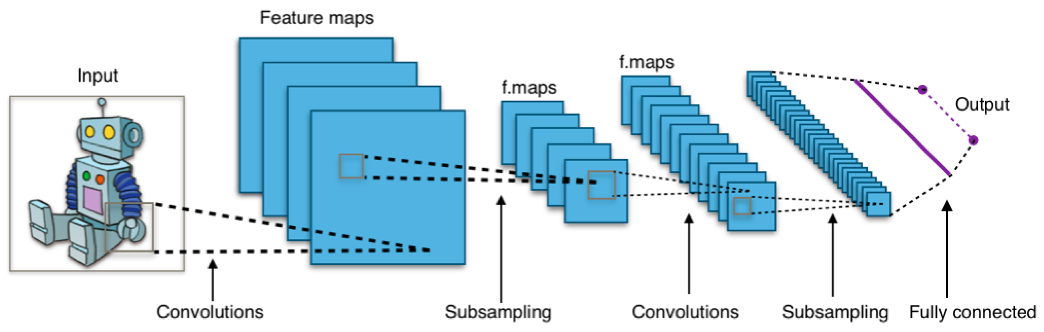
Figure 2.
Working of CNN [81]
Figure 2.
Working of CNN [81]
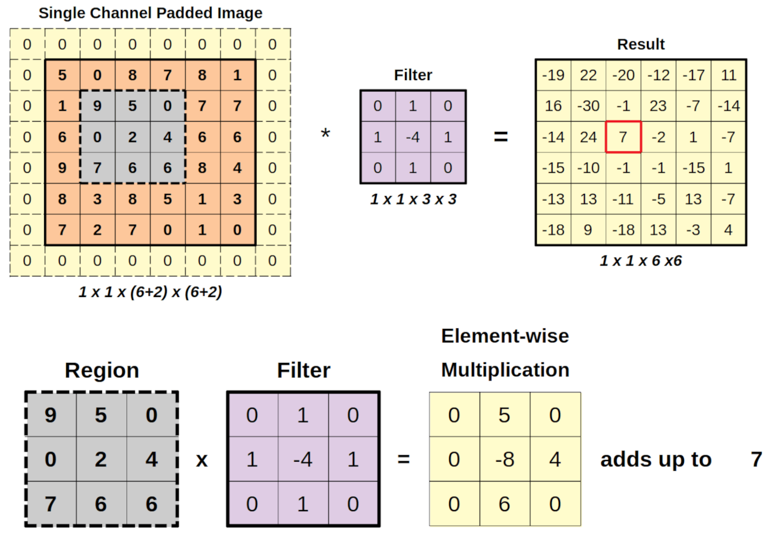
Figure 3.
Architecture of VGG-16 [84]
Figure 3.
Architecture of VGG-16 [84]
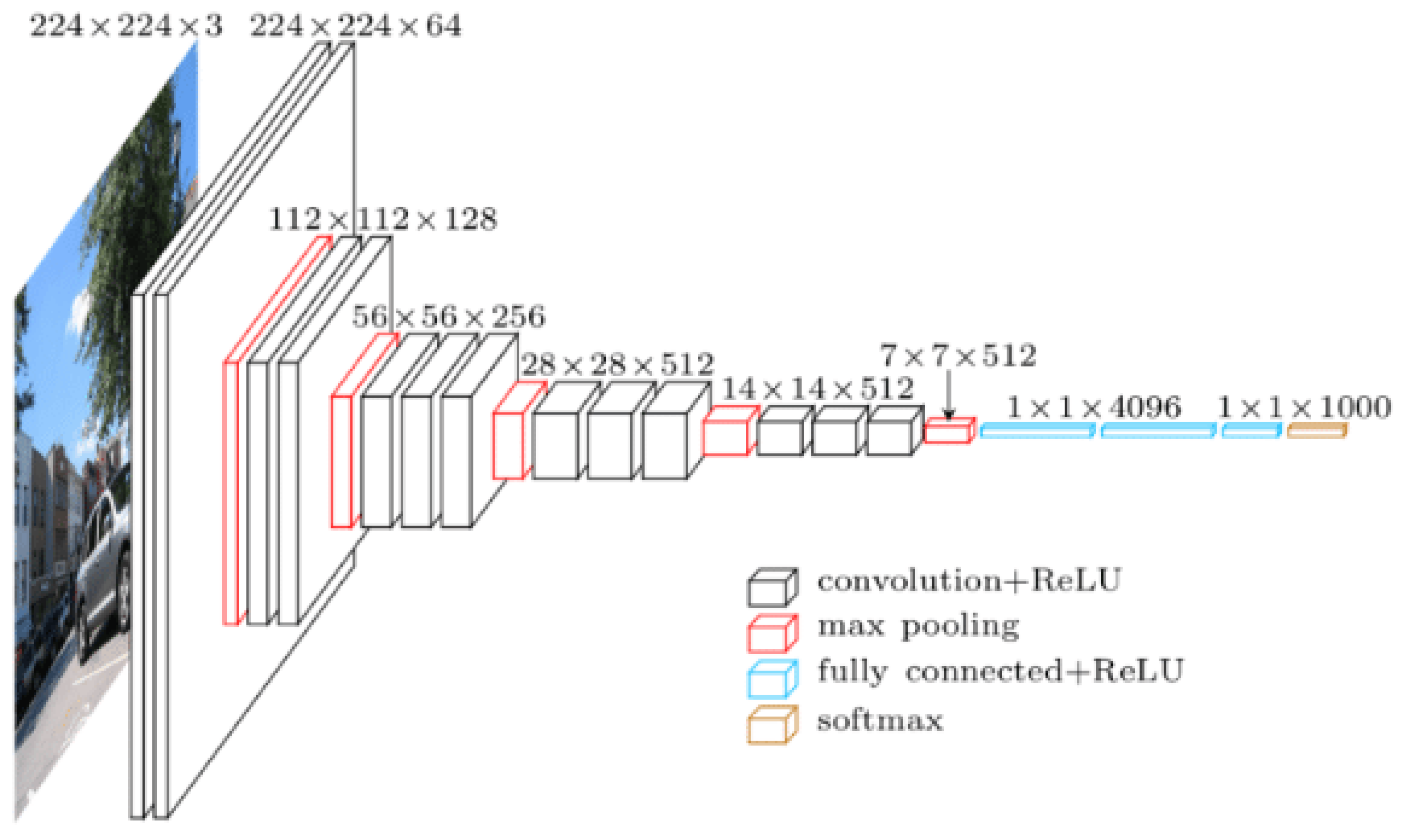
Figure 6.
Architecture of LeNet-5 [95]
Figure 6.
Architecture of LeNet-5 [95]
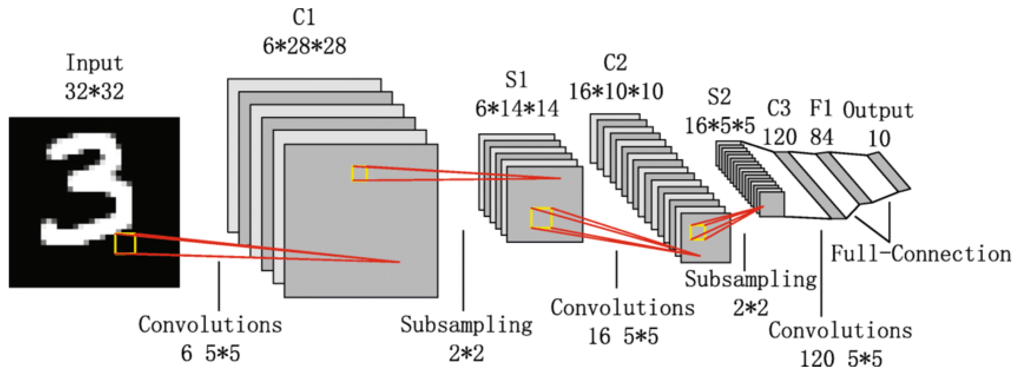
Figure 9.
Residual blocks [106]
Figure 9.
Residual blocks [106]
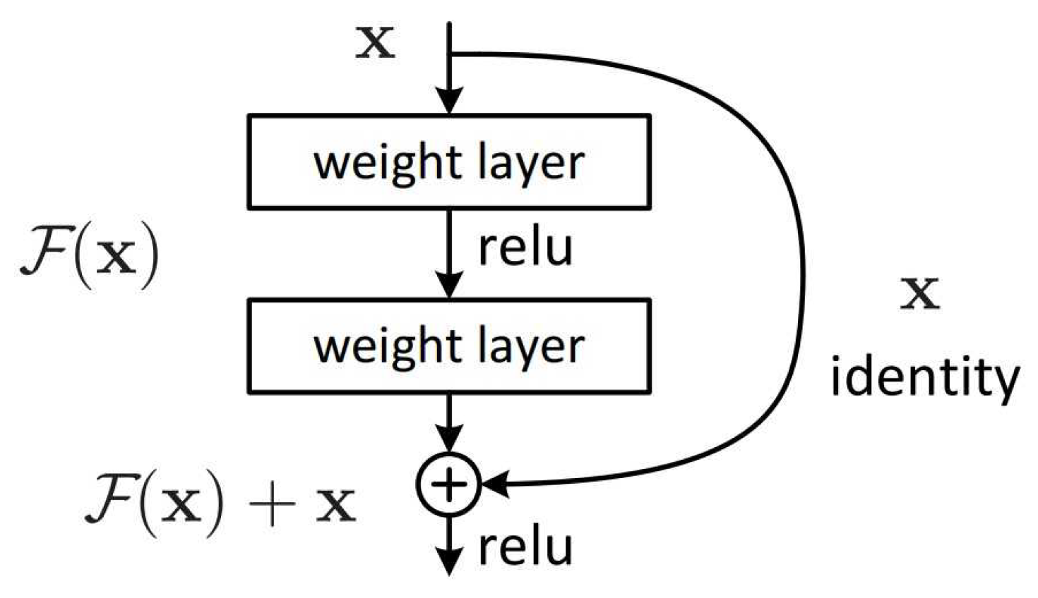
Figure 12.
Architecture of DenseNet [117]
Figure 12.
Architecture of DenseNet [117]
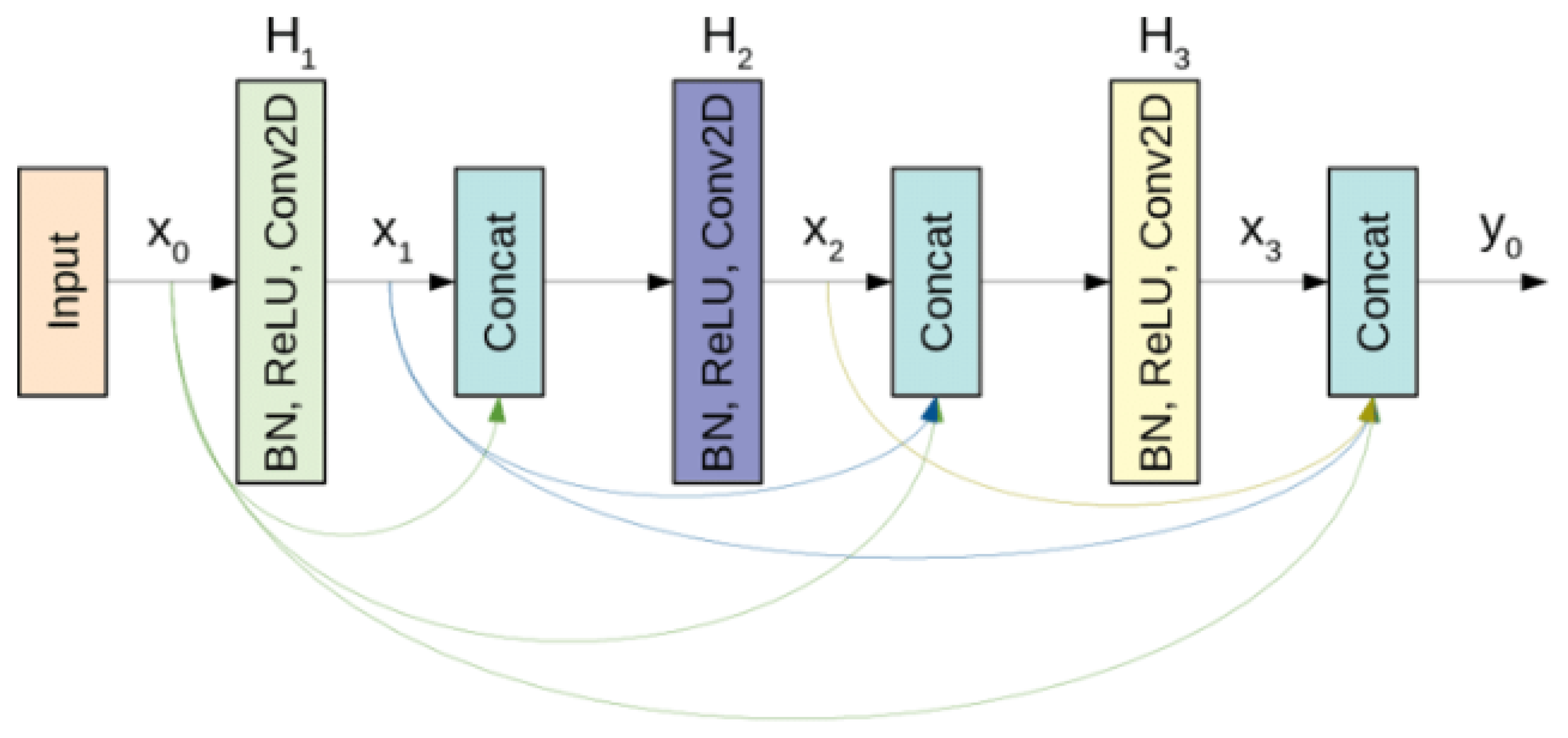
Figure 13.
Architecture of EfficientNet [122]
Figure 13.
Architecture of EfficientNet [122]
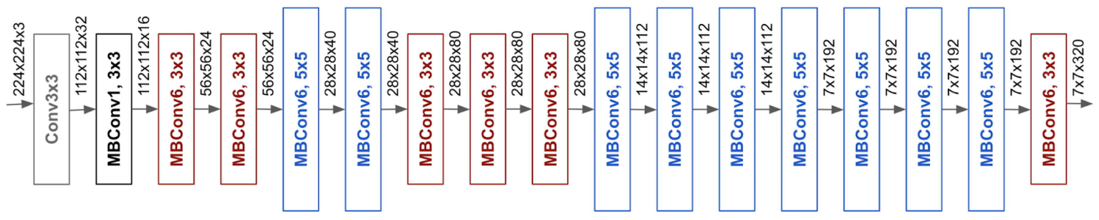
Figure 17.
Precision of CNN models
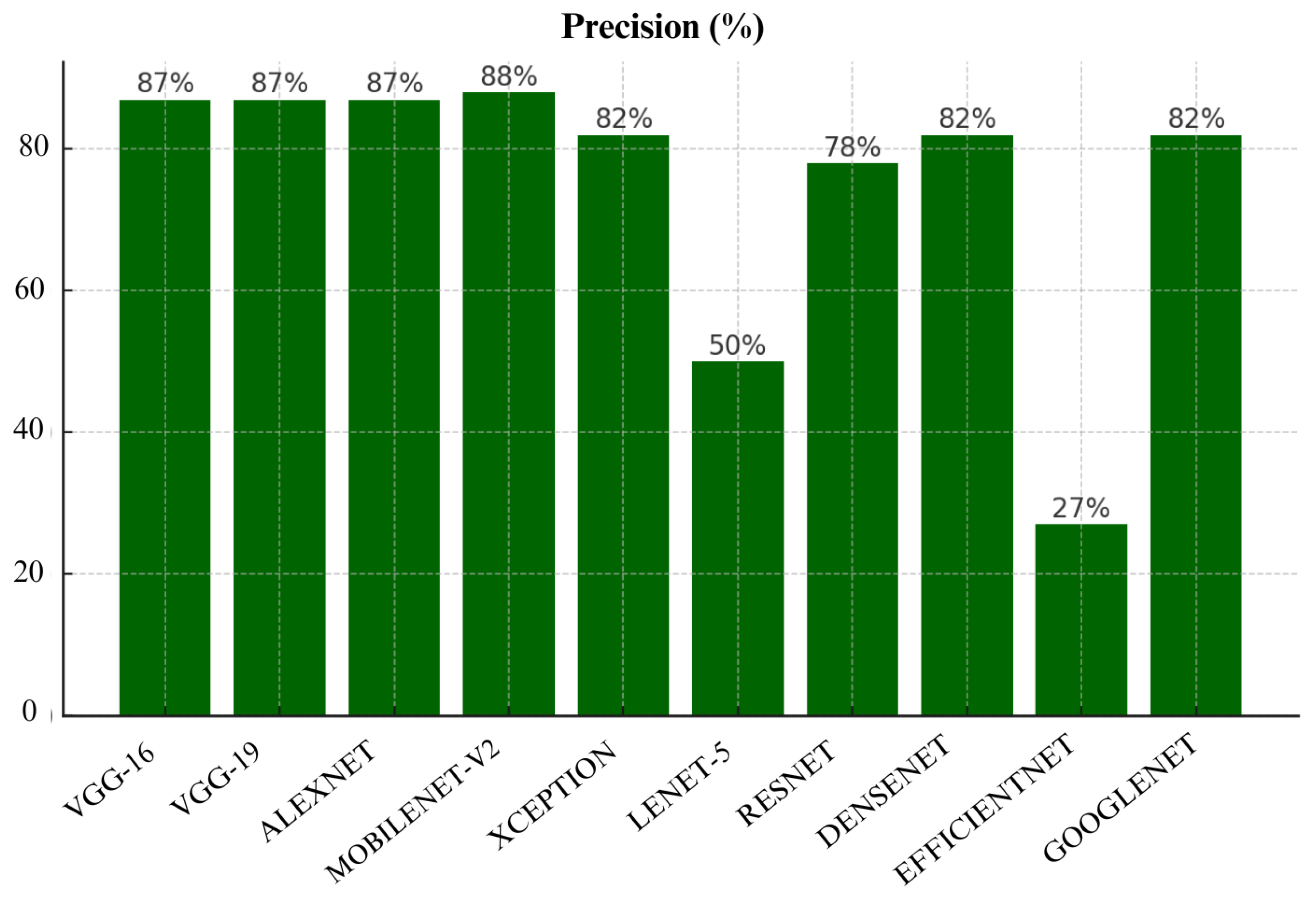
Figure 18.
Recall of CNN models
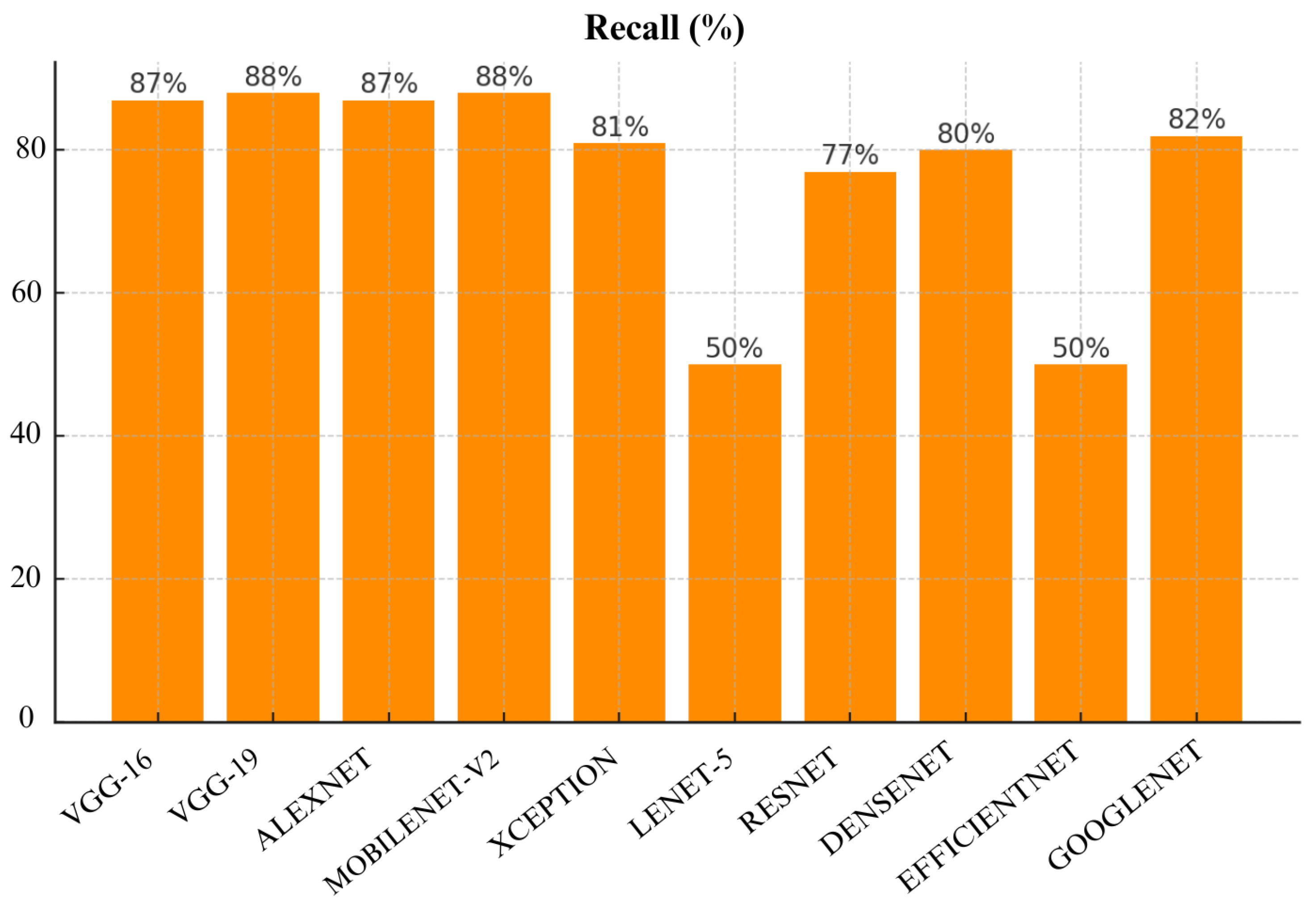
Figure 19.
F1-Score of CNN models
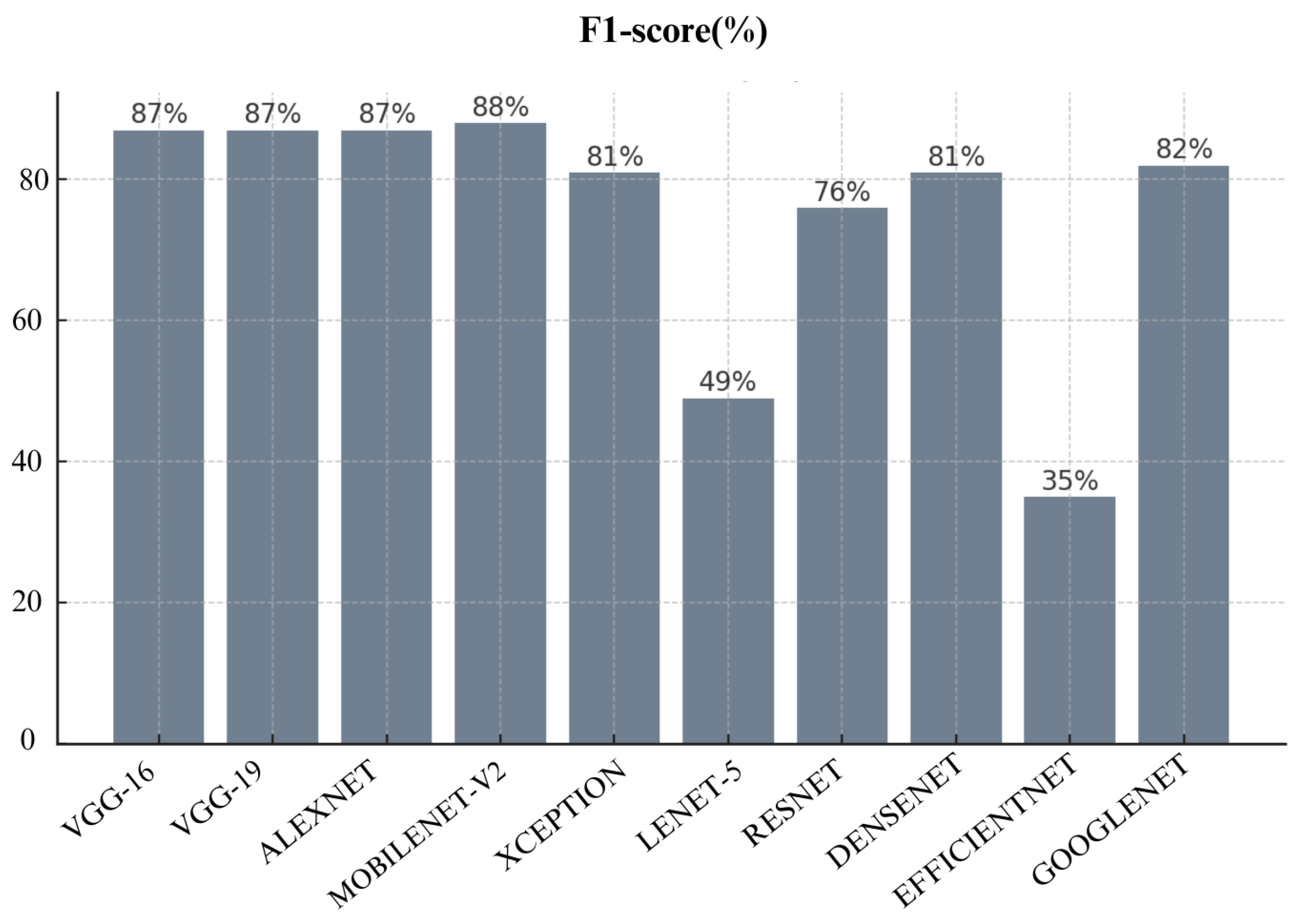
Figure 20.
Specificity of CNN models
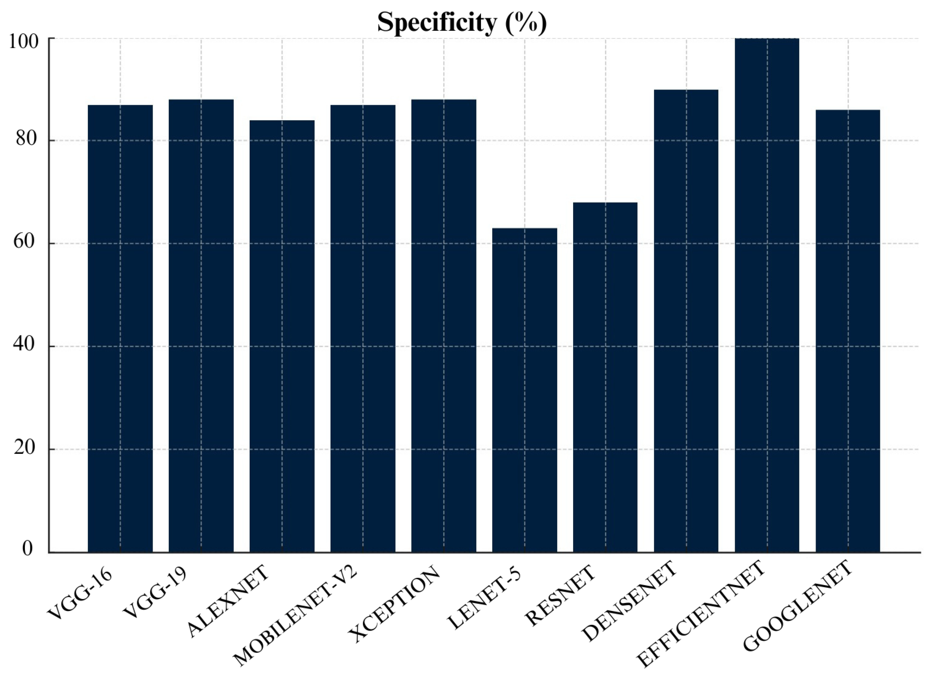
Figure 21.
FPR of CNN models
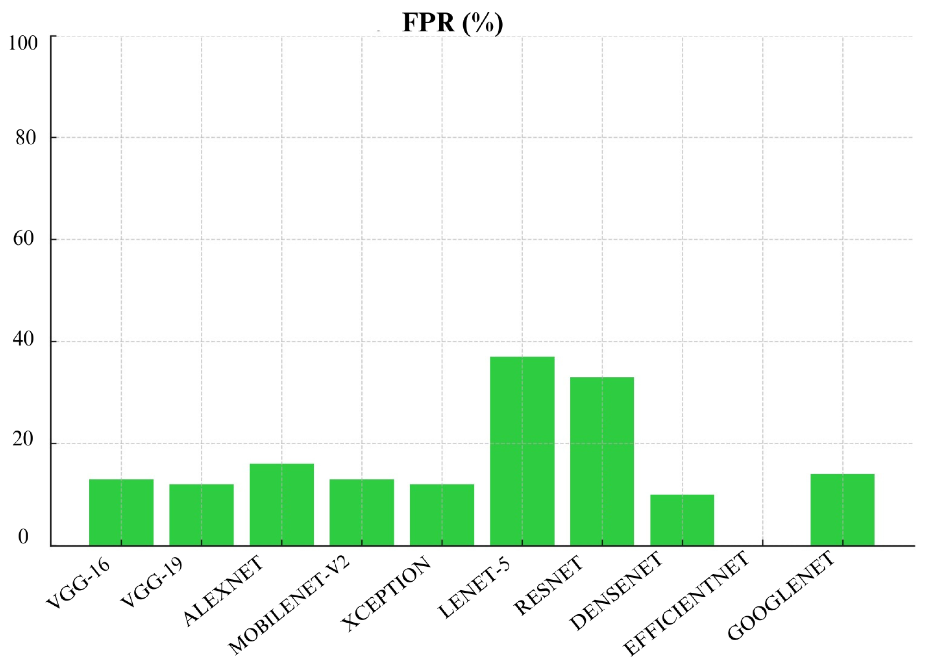
Figure 22.
FNR of CNN models
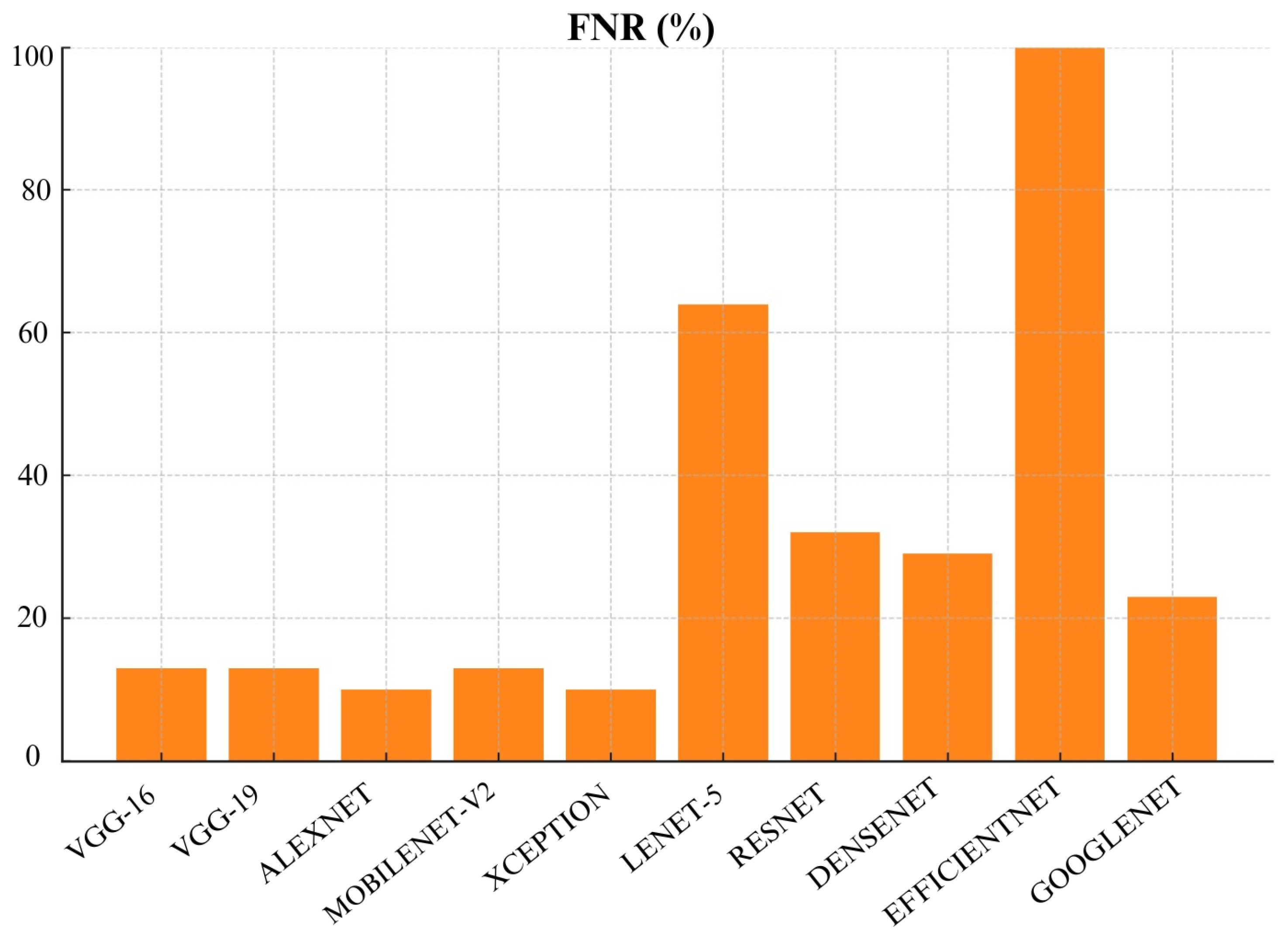
Figure 23.
FDR of CNN models
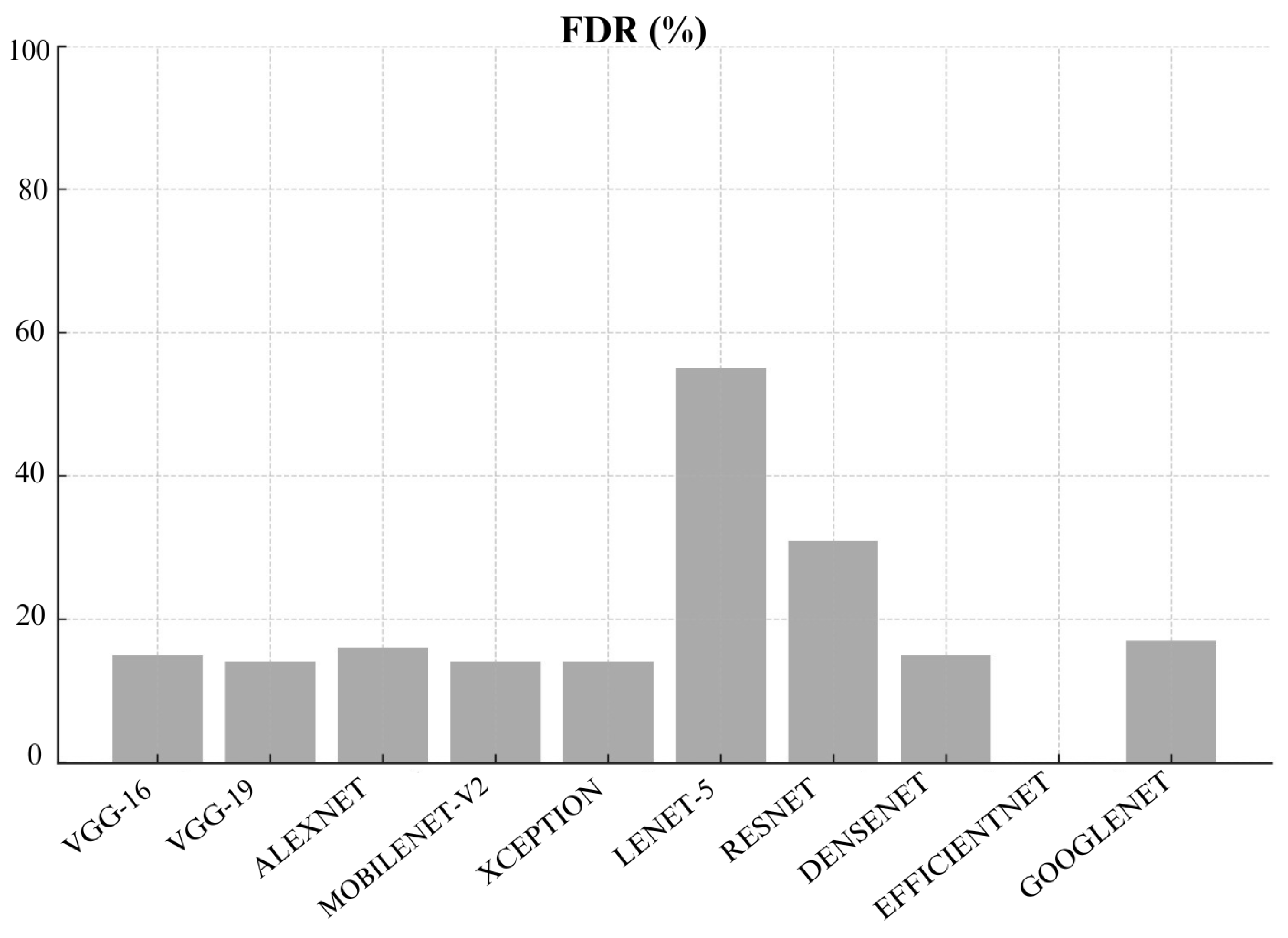
Table 1.
Performance Comparison of CNN Architectures
| Architecture | Accuracy | Precision | Recall | F1-score |
|---|---|---|---|---|
| VGG-16 | 90% [29] | 91% [29] | 90% [29] | 90% [29] |
| VGG-19 | 97% [30] | 86% [31] | 85% [31] | 80% [31] |
| ALEXNET | 99% [32] | 99% [33] | 93% [33] | 96% [33] |
| MOBILENET-v2 | 94% [33] | 98% [33] | 90% [33] | 94% [33] |
| XCEPTION | 93% [29] | 89% [29] | 93% [29] | 93% [29] |
| LENET-5 | 89.7% [29] | 89.5% [29] | 89.5% [29] | 89.5% [29] |
| RESNET | 69% [34] | 92% [34] | 82.3% [34] | 90% [35] |
| DENSENET | 89% [36] | 90% [37] | 88% [37] | 88.94% [37] |
| EFFICIENTNET | 98% [38] | 86% [38] | 86% [38] | 85% [38] |
| GOOGLENET | 93% [39] | 98% [25] | 96% [39] | 97% [39] |
Table 2.
Performance Comparison of CNN Architectures
| Architecture | Specificity | FPR | FDR | FNR | AUC |
|---|---|---|---|---|---|
| VGG-16 | 86.6% [40] | 8.7% [41] | 47% [41] | 50.6% [41] | 81% [41] |
| VGG-19 | 88% [42] | 65.8% [43] | 28% [43] | 11% [43] | 84% [42] |
| ALEXNET | 75.9% [44] | 24% [44] | 23.6% [44] | 9.8% [44] | 92% [45] |
| MOBILENET-v2 | 97% [46] | 48% [43] | 23.5% [43] | 16.5% [43] | 95% [45] |
| XCEPTION | 44.9% [43] | 55% [43] | 25% [43] | 12% [43] | 96%[45] |
| LENET-5 | 89% [29] | 10.4% [29] | 10.3% [29] | 10.3% [29] | 89% [29] |
| RESNET | 100% [47] | 4% [48] | 4% [48] | 3% [48] | 73% [49] |
| DENSENET | 92% [50] | 19% [51] | 22% [51] | 34% [51] | 74% [52] |
| EFFICIENTNET | 91% [38] | 5% [53] | 50% [54] | 7% [53] | 77% [52] |
| GOOGLENET | 100% [32] | 22% [51] | 33% [51] | 28% [51] | 92% [55] |
Table 3.
Datasets commonly used in literature for AI-based skin cancer detection
| Ref | Dataset | Source | No. of Images |
|---|---|---|---|
| [18] | HAM10000 | ISIC ARCHIVE | 11,720 |
| [13] | ISIC-2017 | ISIC ARCHIVE | 2750 |
| [8] | ISIC-2018 | ISIC ARCHIVE | 11527 |
| [18] | PH2 | Hospital Pedro Hispano, Portugal | 200 |
Table 5.
Performance Comparison of CNN Architectures
| Architectures | Accuracy | Precision | Recall | F1-score |
|---|---|---|---|---|
| VGG-16 | 97% | 87% | 87% | 87% |
| VGG-19 | 88% | 87% | 88% | 87% |
| ALEXNET | 87% | 87% | 87% | 87% |
| MOBILENET-v2 | 88% | 88% | 88% | 88% |
| XCEPTION | 82% | 82% | 81% | 81% |
| LENET-5 | 51% | 50% | 50% | 49% |
| RESNET | 77% | 78% | 77% | 76% |
| DENSENET | 81% | 82% | 80% | 81% |
| EFFICIENTNET | 55% | 27% | 50% | 35% |
| GOOGLENET | 82% | 82% | 82% | 82% |
Table 6.
Performance Comparison of CNN Architectures
| Architectures | Specificity | FPR | FNR | FDR | AUC |
|---|---|---|---|---|---|
| VGG-16 | 87% | 13% | 13% | 15% | 87% |
| VGG-19 | 88% | 12% | 13% | 14% | 88% |
| ALEXNET | 84% | 16% | 10% | 18% | 87% |
| MOBILENET-v2 | 87% | 13% | 10% | 10% | 88% |
| XCEPTION | 88% | 12% | 26% | 16% | 81% |
| LENET-5 | 63% | 37% | 64% | 55% | 50% |
| RESNET | 68% | 33% | 13% | 31% | 77% |
| DENSENET | 90% | 10% | 29% | 15% | 80% |
| EFFICIENTNET | 100% | 0% | 100% | 0% | 50% |
| GOOGLENET | 86% | 14% | 23% | 17% | 82% |
Disclaimer/Publisher’s Note: The statements, opinions and data contained in all publications are solely those of the individual author(s) and contributor(s) and not of MDPI and/or the editor(s). MDPI and/or the editor(s) disclaim responsibility for any injury to people or property resulting from any ideas, methods, instructions or products referred to in the content. |
© 2024 by the authors. Licensee MDPI, Basel, Switzerland. This article is an open access article distributed under the terms and conditions of the Creative Commons Attribution (CC BY) license (http://creativecommons.org/licenses/by/4.0/).
Copyright: This open access article is published under a Creative Commons CC BY 4.0 license, which permit the free download, distribution, and reuse, provided that the author and preprint are cited in any reuse.


