Submitted:
12 December 2024
Posted:
15 December 2024
You are already at the latest version
Abstract
Incorrect sensor readings can cause serious problems in Wireless Sensor Networks (WSNs), potentially disrupting the operation of the entire system. As shown in the literature, they can arise from various reasons; therefore, addressing this issue has been a significant challenge for the scientific community over the past few decades. In this paper, we examine the applicability of five distributed consensus gossip-based algorithms for sensor fusion (namely, the Randomized Gossip algorithm (RG), the Geographic Gossip algorithm (GG), the Broadcast Gossip algorithm (BG), the Push-Sum protocol (PS), and the Push-Pull protocol (PP)) to compensate for incorrect data in WSNs. More specifically, we consider a scenario where the sensor-measured data (measured by a set of independent sensor nodes) are skewed due to Gaussian noise with a various standard deviation, resulting in discrepancies between the measured values and the true value of observed physical quantities. Subsequently, the aforementioned algorithms are employed to mitigate this skewness in order to improve the accuracy of the measured data. In this paper, WSNs are modelled as random geometric graphs (RGGs) with various connectivity, and the performance of the algorithms is evaluated using two metrics (specifically, the mean square error (MSE) and the number of sent messages required for an algorithm to be completed). Based on the presented results, it is identified that all the examined algorithms can significantly suppress incorrect sensor readings, and the best performance is achieved by PS in dense graphs and by GG in sparse graphs. Additionally, the performance of the analyzed distributed consensus gossip algorithms is compared to the best deterministic consensus algorithm applied for the same purpose.
Keywords:
consensus
; data aggregation
; distributed computing
; Gaussian noise
; gossip algorithms
; incorrect data
; information aggregation
; information fusion
; sensor fusion
; sensor networks
1. Introduction
In this section, we provide a theoretical insight into the subjected topic. It is divided into four subsections, as follows:
- Wireless sensor networks (SubSection 1.1) – in this subsection, we discuss WSNs, including their sensor nodes, common architectures, real-world applications, as well as the key advantages and disadvantages of this technology.
- Sensor Fusion in Wireless Sensor Networks (SubSection 1.2) – we describe fundamental concepts, the key benefits of sensor fusion, the differences between centralized and distributed schemes, consensus algorithms, and their applications in real-world scenarios.
- Our Contribution (SubSection 1.3) – in this subsection, we highlight our contribution and provide a justification for it.
- Paper Organization (SubSection 1.4) – this section provides an overview of how the paper is structured into sections and subsections.
1.1. Wireless Sensor Networks
WSNs, a key component of the Internet of Things (IoT), are a contemporary information technology for remotely monitoring and controlling various physical environments [1,2,3]. They are formed by (potentially) hundreds to thousands of spatially distributed autonomous tiny entities (known as sensor nodes) that communicate with each other via wireless channels and operate in possibly highly noisy environments (see Figure 1 for the architecture of sensor nodes) [4,5]. These sensor nodes are capable of sensing various physical quantities from their surroundings (e.g., temperature, sounds, pollution, wind, blood pressure, light intensity, etc.) whereby WSNs have attracted considerable attention from both academia and industry over the past few decades [6,7,8,9,10,11].
As discussed in [12,13,14], WSNs support a variety of standards and protocols, including Zigbee, BLE, LoRa, IEEE 802.15, etc. These networks are typically structured in an architecture where sensor nodes continuously monitor specific physical quantities from their surrounding environment and transmit the collected data to a base station [15]. The base station supervises the other nodes and relays relevant information to end users via the Internet (see Figure 2 for the typical architecture of WSNs) [15].
As shown in the literature [16,17,18,19,20,21,22,23], WSNs have plenty of advantages, thereby finding a wide range of applications across various fields such as health care, security, environmental monitoring, agriculture, industry, forest fire detection, animal tracking, flood detection, etc. Below, we focus on the most notable advantages of WSNs [24,25,26,27,28,29]:
- ⋄
- Scalability: means that sensors can be easily added to and removed from a network. Thus, high scalability allows for an effective increase or decrease in the number of sensor nodes without degrading the performance stability and reliability.
- ⋄
- Financial affordability: one of the most critical design considerations for WSNs is keeping sensor production costs low. Thus, WSN-based applications are typically cost-effective in spite of the deployment of numerous sensor nodes in real-world applications.
- ⋄
- Energy efficiency: algorithms and sensor nodes are designed to enable long operation of WSNs without any maintenance (or with minimal maintenance). As a result, the network lifetime of WSNs is significantly extended, allowing for their widespread use in vast and hard-to-reach areas.
- ⋄
- Monitoring in real-time: sensor nodes can reliably sense the current status of monitored physical quantities, thereby providing topical information on these quantities and enhancing data collection and decision-making processes.
- ⋄
- Infrastructure-less architecture: this feature guarantees a simplified deployment and redeployment of sensor nodes, as well as their seamless reconfiguration.
- ⋄
- Compatibility: WSNs are compatible with a variety of devices and innovative plug-ins, enhancing their applicability across multiple domains.
As stated above, sensor nodes are typically cheap, tiny, and low-power devices, which limits many of their capabilities [30]. These limitations lead to many drawbacks of WSNs, with the most significant ones outlined below [31,32,33,34,35,36,37]:
- ⋄
- Signal interference: communication between sensor nodes can be easily disturbed by other wireless-based technologies, leading to a degradation in the quality of communication within WSNs.
- ⋄
- Limited power source: is caused by the reliance of sensor nodes on battery power (recharging or replacing batteries can be challenging in many real-world applications). This can prevent sensor nodes from performing demanding computational tasks.
- ⋄
- Low memory capabilities: negatively affect the reliability, efficiency, and functioning of WSNs.
- ⋄
- Security issues: data confidentiality may be compromised since securing WSNs is a challenging task due to their energy, memory, and computation constraints.
- ⋄
- Constrained transmission range: a limited transmission range of sensor nodes can cause serious problems within large-scale environments and areas with barriers that may interfere with wireless communication (e.g., walls, high buildings, etc.).
- ⋄
- Narrow bandwidth: degrades the communication speed in WSN-based applications.
- ⋄
- Limited sensing capabilities: due to the use of inexpensive hardware components, sensor nodes may struggle to accurately sense their surrounding environment since external factors are transduced into a measured value.
As a result of the previously discussed drawbacks, sensor nodes are susceptible to various environmental factors (e.g., temperature fluctuations, rain, radiation, pressure variations, chemical exposure, dust, electrical interference, etc.) that can significantly impair their performance or even lead to failures [38,39]. As discussed in [40], sensor readings are also affected by other external devices, hardware noise, improper measurement techniques, etc. Furthermore, WSNs are susceptible to attacks by hackers and cybercriminals (e.g., jamming, eavesdropping, spoofing, wormholes, etc.) and must contend with challenges such as high data redundancy, data duplicity, quantized computing, etc. [38,41,42]. Therefore, as indicated in the literature [38,39,40,41,42], many researchers have dedicated their efforts to addressing these drawbacks of WSNs over the past decades.
In this paper, we address the issue of how to struggle with incorrect sensor readings caused by negative environmental factors and other factors skewing the measured data. We model these factors as Gaussian noise skewing the data measured by sensor nodes. Thus, the measured data differ from the true value of the sensed physical quantity due to this noise. We assume that noise is an independent and identically distributed (IID) random variable with the Gaussian distribution that skews the initial inner state at each sensor node in WSNs. More specifically, we focus our attention on the applicability of distributed consensus gossip algorithms for data aggregation to suppress the impact of incorrect sensor readings.
1.2. Sensor Fusion in Wireless Sensor Networks
In general, the term "sensor fusion" is understood as a process of integrating data measured by multiple independent sensor nodes in order to generate detailed and complete information about the monitored environment or process of interest [43]. In other words, an output of sensor fusion allows a better understanding of the observed quantity and reduces the amount of uncertainty [44]. This means that fused data provides us with more consistent, more accurate, and more dependable information about the observed quantity than a single data source would. The application of sensor fusion can also allow WSNs to execute the same goals even if one or more sensor nodes are removed from WSNs. Moreover, due to sensor fusion, WSNs can fulfill novel functionalities without adding new sensor nodes. As discussed in [45,46,47], the usage of sensor fusion can be highly beneficial in many real-world scenarios since it may effectively compensate for failures, noise, data redundancy, etc. In Figure 3, a general architecture of sensor fusion in WSNs is depicted [48].
In this paper, we focus on a distributed sensor fusion scheme, where the sensor nodes are not aware of network topology [49]. Besides, no central unit to coordinate the whole process is required in these schemes (in contrast to old-fashioned centralized schemes, where a data fusion center is responsible for data collection). Therefore, distributed sensor fusion is a much more effective solution than centralized schemes, especially in mobile and power-constrained technologies (such as WSNs). In distributed schemes, only the adjacent sensor nodes are required to communicate with each other, and sensor nodes update their states according to local rules. The final goal of each sensor node is to possess at least a precise estimate of the aggregated quantity.
As mentioned earlier in this paper, we focus our attention on distributed consensus gossip-based algorithms for sensor fusion. A consensus is understood as a general agreement achieved among a group of entities [50]. In general, the term ’consensus algorithm’ is considered to be an iterative mechanism used to reach agreement (through local interactions) on a single value among involved entities with different initial values. As shown in the literature [51,52,53,54,55], consensus algorithms are applicable for various purposes (leader election, decision processes, cryptocurrency transactions, data replication, data aggregation, load balancing, state estimation, network size estimation, etc.) and find the usage in numerous fields (blockchain, sensor networks, UAVs, big data analysis, etc.). In this paper, we are concerned with gossip-based algorithms, i.e., the selection of the transmitting node/the message receiver is stochastic, which ensures effective information diffusion across WSNs.
1.3. Our Contribution
Our contribution in this paper is to examine the applicability of five frequently applied distributed consensus gossip algorithms for sensor fusion (namely, RG, GG, BG with three initial configurations, PS, and PP) to compensate for incorrect data in noisy WSNs. More specifically, we assume that sensor readings are significantly affected by negative environmental factors, worsening the precision of the measurements (see Figure 4 for an example of incorrect sensor readings). As a result, the measured data of every sensor node differs from the true value of the observed physical quantity, which may affect the operation of WSNs [38]. Our hypothesis is that the application of sensor fusion performed by the mentioned algorithms can ensure a significant increase in the precision of the measured data and improve decision-making. The performance of the examined algorithms is tested in RGGs and evaluated by two metrics (MSE and the number of sent messages required for an algorithm to be completed).
1.4. Paper Organization
The rest of this paper is organized as follows:
- Section 2 (Related Work) – in this section, we provide a list of the most recent and best-cited papers dealing with how to suppress incorrect sensor readings in sensor networks.
- Section 3 (Theoretical Background) – this section is divided into three subsections and focuses on the theoretical background of the topic. Specifically, we introduce the applied graph model (RGGs), the model of incorrect sensor readings, the used stopping criterion, and the examined algorithms.
- Section 4 (Applied Research Methodology and Metrics) – introduces the applied research methodology and the metrics used to evaluate the performance of the examined algorithms.
- Section 5 (Experiments and Discussion) – consists of the experimental results obtained using MATLAB 2018b, along with a discussion of observable phenomena.
2. Related Work
In this paragraph, we turn our attention to papers dealing with techniques to suppress incorrect sensor readings in WSNs. Over the past decades, many authors have addressed this issue and proposed various techniques for this purpose. We focus on relevant papers with a high citation rate and papers that have been published recently.
In [56], the authors deal with incorrect readings caused by improper hardware design and calibration. Also, they address how sensor nodes with low remaining power energy can cause incorrect sensor readings. In the paper, the authors discuss that it is not always feasible to ensure a flawlessly configured sensor network; therefore, they recommend automated detection, classification, root-cause analysis, and techniques to scrub collected data from the sensor nodes.
The authors of [57] propose a technique to predict future states of the observed physical quantity, which can compensate for previously executed incorrect sensor readings. The authors apply an O(n2log(n)) algorithm for the linear prediction problem. This algorithm is capable of calculating the solution from the input sensor readings without determining the planar configuration.
Paper [58] presents a Bayesian approach to reduce the data-associated uncertainty. The presented approach combines prior knowledge of correct sensor readings, noise characteristics, and incorrect sensor readings in order to increase the precision of the measured data. This cleaning is executed by either sensor nodes or the base station.
In [59], a self-validating strategy for multifunctional sensors is proposed. The approach exploits the Grey Bootstrap model, which can generate a prediction model. This bootstrap method ensures that the uncertainty can be estimated without prior information about the distribution of the measured data. In this strategy, a measured value is compared to a predicted value, allowing suppression of incorrect sensor readings.
The authors of [60] propose an in-situ calibration method. Here, the benchmark is established based on observation of the monitored environment. The sensor-measured data are subsequently compared to this benchmark and modified.
The paper [61] introduces a method based on the Kalman Filter, autoregressive integrated moving average, knowledge-based systems, and smoothing operators. The method is capable of detecting and correcting data with anomalous features.
An easily configurable scheme based on local predictors and listening to correlated adjacent nodes is proposed in [62]. In this scheme, sensor nodes compare the confidence of the sensed value with the output generated by the predictor.
The authors of [63] propose SNRepair, a self-calibrating mechanism based on deep reinforcement learning. The incorrect readings can be calibrated according to historical healthy data in a few seconds. In the experimental section, it is identified that the mechanism can operate with high precision even in highly noisy environments.
The approach in [64] utilizes statistical time series analysis with Pearson’s correlation or dynamic time warping coupled with a data-driven algorithm in convolutional neural networks. The authors apply effective statistical methods to identify the most appropriate sensors to predict prior to the computationally intensive training of complex machine learning models.
In [65], the application of average consensus algorithms with the Perron matrix to compensate for incorrect data is investigated in several WSN scenarios. Namely, the Graph Order weights, the Maximum Degree weights, and the Best Constant weights are applied to compensate for Gaussian noise skewing the measured data. From the results, it is seen that all algorithms can significantly suppress Gaussian noise, thereby optimizing MSE in every examined scenario. The best performance is achieved by the Best Constant weights, but no difference among the examined algorithms is observed for many configurations of the applied stopping criterion.
The paper [66] is focused on the applicability of the Metropolis-Hastings with various initial configurations to suppress or even overcome Gaussian noise affecting the sensor readings in WSNs. In the paper, it is identified that the algorithm can significantly suppress noise for each scenario. However, it is outperformed by the best-performing algorithm with the Perron matrix (i.e., the Best Constant weights). Besides, one can see that the initial configuration of the Metropolis-Hastings algorithm has either marginal or no impact on the estimation precision.
Thus, we can see that no other paper deals with the applicability of distributed consensus gossip algorithms for sensor fusion to compensate for incorrect sensor readings. This paper follows on from our previous papers [65,66], where two deterministic consensus algorithms are applied for the same purpose. Accordingly, we also compare the performance of the top gossip algorithms with that of the best-performing deterministic consensus algorithm.
3. Theoretical Background
This section is divided into three subsections as follows:
- Random Geometric Graphs (SubSection 3.1) – in this subsection, we introduce the used mathematical model to model WSNs (RGGs).
- Insight into Distributed Consensus Gossip-based Sensor Fusion in Wireless Sensor Networks (SubSection 3.2) – this subsection provides the model of incorrect sensor readings, insight into distributed consensus gossip sensor fusion, and the applied stopping criterion.
- Examined Distributed Consensus Gossip Algorithms (SubSection 3.3) – here, we introduce five algorithms chosen for evaluation in this paper.
3.1. Random Geometric Graphs
In this paper, we model WSNs as undirected, simple, finite graphs G with connected topologies determined by the vertex set V and the edge set E (i.e., G = (V,E)) [67,68]. The vertex set V comprises all vertices in G, each representing a sensor node in WSN. The vertices are distinguishable by a unique index i = 1,2..., n (i.e., V = (v1, v2,... vn)), where n (n = |V|) represents the graph order, or in other words, the number of sensor nodes in WSN. The edge set E⊂V×V consists of all graph edges in G, which represent a direct (one-hop) link between two vertices (i.e., two corresponding sensor nodes can directly communicate with one another). An edge labeled as eij links vertices vi and vj. The cardinality of this set (|E|) equals the graph size, i.e., the number of direct connections in WSN. See Figure 5 for an example of an undirected simple finite graph with n = 14 and |E| = 16.
In this paper, we use RGGs, a commonly used graph model for representing systems such as WSNs, IoT, social networks, etc. [69,70]. In RGGs, vertices are randomly placed within a finite square area, and an edge connects each pair of vertices if the distance between them is less than a specified transmission radius, which is uniform across all vertices. To produce graphs with various connectivity, we modify the transmission radius.
3.2. Insight into Distributed Consensus Gossip-based Sensor Fusion in Wireless Sensor Networks
As mentioned above, we consider a scenario where a set of spatially distributed sensor nodes measure a physical quantity (let us label the true value of this quantity as ) from their surrounding environment. However, due to factors discussed in SubSection 1.1, sensor readings deviate from the true value of . Thus, the initial inner state xi(0) of vi is defined as follows [65,66]:
Here, zi is an IID random variable of Gaussian distribution (representing noise skewing sensor data), defined as follows [65,66]:
Here, the symbol presents the mean (equal to zero when modeling noise), and the symbol denotes the standard deviation. As shown in the literature, modeling incorrect sensor readings as in (1) is common across many scenarios [71,72].
In order to justify our hypothesis that distributed consensus gossip algorithms for sensor fusion may be applied to suppress Gaussian noise, we show how sensor fusion (RG is applied) can alleviate incorrect sensors in a random simple topology formed by five vertices (Figure 6), and the evolution of inner states when data are skewed due to Gaussian noise (Figure 7).
Communication among sensor nodes in WSNs is coordinated—depending on the applied gossip algorithm—by either a single global clock or n local clocks [73]. Each time the clock ticks, specific steps defined by the applied algorithm are executed, referred to as a time instance k. We denote the inner state of vi at time instance k as xi(k), and a column vector that gathers the inner states of all sensor nodes at time instance k as x(k).
As previously mentioned, the operation of the tested algorithm is bounded by a stopping criterion to optimize execution time. In the experimental section, we apply the stopping criterion defined in (3), based on the comparison between the highest and lowest current inner states (from all nodes) at time instance k [73].
Once the condition (3) is met for the first time, the algorithm is considered complete and ceases execution. The applied stopping criterion is configurable by setting the value of P; higher values are assumed to ensure higher precision of the final inner states, albeit at the cost of slowing down the algorithms [73]. In Figure 8, we show how MSE and the number of sent messages differ in a random simple topology when the value of P is modified (PS is applied).
3.3. Examined Distributed Consensus Gossip Algorithms
As previously mentioned in this paper, we examine how five widely used distributed consensus gossip algorithms can mitigate the effects of incorrect sensor readings.
One of these is the RG algorithm [74], which has been identified as a vulnerable solution that requires a significant volume of transmitted messages. Its principles can be described as follows: each sensor node is equipped with its own local clock, which ticks at random intervals. At each time instance k, the sensor node whose clock has ticked (denoted as vi) selects one of its neighbors, labeled as vj, uniformly at random for pairwise averaging described below:
At this time instance, the inner states of all other sensor nodes remain unchanged.
The next tested algorithm is GG [75], which utilizes geographic routing to optimize sensor fusion. This approach increases the diversity of pairwise exchanges; however, sensor nodes must be aware of the geographical positions of other nodes in WSN. Like in RG, each sensor node has its own local clock that ticks randomly. At each time instance k, one of the sensor nodes (vi) is activated and randomly selects, according to a uniform distribution, one of the other nodes in the entire network (vj) for pairwise averaging, not just from adjacent nodes, as is the case with RG.
In this paper, we also evaluate BG [76], an algorithm that does not rely on pairwise communication, in contrast to the two previous algorithms. However, the precision of this algorithm may be significantly lower, potentially limiting its usability in certain scenarios [73]. The principle of this algorithm is as follows: the sensor nodes are equipped with local clocks once again. When the clock of a node ticks (vi), it sends its current inner state to all adjacent neighbors (vj), which then apply the following update rule:
Here, the parameter can take values from:
The node (vi) and any nodes that have not received a message from it at this time instance do not update their inner states.
Another examined algorithm is PS, which functions correctly only if the total system mass remains constant, as noted in [77]. Consequently, this approach is significantly vulnerable to message losses. In this algorithm, each node maintains and regularly updates two variables: the state si(k) (initialized by local measurements) and the weight wi(k) (initialized to one). At each time instance k (all sensor nodes are synchronized by a single global clock), every node randomly selects one of its neighbors and sends half of both its current inner state and weight. The same values are also stored in its internal memory. The arithmetic mean estimate can be easily calculated at each node as follows:
Each sensor node can then compute the value of its inner state for k+1 as the sum of half of its current state and the states received at k. The weights for the next time instance are determined in a similar manner.
The final algorithm to be tested is PP [78], in which the sensor nodes are once again synchronized by a single global clock. Whenever this clock ticks, each sensor node sends its current inner state (i.e., a Push message) to a randomly chosen neighbor, selected with a uniform distribution. This neighbor then replies by sending its current state (i.e., a Pull message). Consequently, these two sensor nodes can perform the pairwise averaging defined in (4).
4. Applied Research Methodology and Metrics
In this section, the applied research methodology and the metrics used to evaluate the algorithms are introduced. As mentioned above, we use the stopping criterion defined in [73] and described in SubSection 3.2 to bound the execution of the algorithms. This stopping criterion is determined by the parameter P, which takes the following values in our experiments:
- ⋄
- P = 10−1
- ⋄
- P = 10−2
- ⋄
- P = 10−3
- ⋄
- P = 10−4
As previously mentioned, we model incorrect sensor readings as Gaussian noise with = 0 and with set as follows:
- ⋄
- = 1
- ⋄
- = 5
To ensure the high credibility of the presented results, we generate 100 sets of unique initial inner states and 100 graphs (for each connectivity) with the graph order n = 30. In the experimental part, we analyze the algorithms in RGGs of either dense (DEN) or sparse (SPAR) connectivity (see Figure 9 for an example of both graph types). Only connected graphs are used in our experiments.
As mentioned earlier in this paper, we apply two metrics to evaluate the performance of the tested algorithms. Specifically, we measure the number of sent messages for an algorithm to complete and MSE (see (8)), a reasonable metric to quantify the precision of the sensor fusion estimation [79,80].
Here, kl is the label of the last time instance, i.e., the instance at which an algorithm is completed. In the experimental part, we repeat each algorithm 100 times in each topology (as the algorithms are stochastic), and only the median of a corresponding metric is depicted in the figures.
As discussed in SubSection 3.3, BG can be adjusted by setting . In our experiments, we set its value to:
- ⋄
- = 0.1 (later referred to as BG 1)
- ⋄
- = 0.5 (later referred to as BG 2)
- ⋄
- = 0.9 (later referred to as BG 3)
5. Experiments and Discussion
In this section, we present the experimental results obtained using MATLAB 2018b and discuss the observable phenomena. As mentioned earlier in this paper, we vary the initial configuration of the applied stopping criterion, the connectivity of RGGs, and of the Gaussian noise. The performance of the algorithms is quantified using two metrics (MSE and the number of sent messages), and the best-performing algorithms are compared against the distributed consensus deterministic Best Constant weights.
In the first analysis, we analyze MSE in densely connected RGGs for various precisions of the applied stopping criterion if = 1. As shown in Figure 10, the value of P has only a marginal effect on the precision of all tested algorithms (only for P = 10E-01, the precision is a bit lower) except on BG. Regardless of further decreases in P, the error of all four algorithms does not drop below -24.87 dB. RG achieves the error in the range [-24.37, -24.87] dB, GG in [-24.32, -24.87] dB, PS in [-24.48, -24.87] dB, and PP in [-24.61, -24.87] dB. Thus, in terms of estimation precision, the choice of any of these four algorithms is almost inconsequential. Unlike in Figure 9, where MSE is analyzed in an error-free scenario, the value of P has only a minor impact on MSE (except on BG). Furthermore, the precision of BG is lower but improves as increases. For , the precision is relatively high, making it highly suitable for real-world applications (with a maximum precision of -17.40 dB). A decrease in P leads to lower MSE when BG is applied. BG 1 achieves the error in the range [-3.15, -5.32] dB, BG 2 in [-7.62, -9.94] dB, and BG 3 in [-16.58, -17.40] dB. The most notable observation is that each algorithm can substantially compensate for incorrect sensor readings (MSE = -0.42 dB without a sensor fusion mechanism). Consequently, their application proves to be highly effective in suppressing Gaussian noise.
In sparsely connected RGGs (Figure 11), MSE of RG, GG, PS, and PP cannot drop below -24.87 dB, consistent with the findings from the previous analysis. Once again, the value of P has little to no impact on MSE when any of these four algorithms are applied. RG achieves errors in the range of [-23.89, -24.87] dB, GG in [-24.32, -24.87] dB, PS in [-23.88, -24.87] dB, and PP in [-23.71, -24.87] dB (their performances do not differ notably from each other). Thus, the connectivity of graphs has only a marginal impact on the performance of these algorithms (except for BG) when used to suppress Gaussian noise. If BG is applied, the precision of sensor fusion is consistently lower than that of the other tested algorithms. However, its precision improves compared to the first analysis, with MSE ranges as follows: BG 1: [-5.85, -6.78] dB, BG 2: [-11.67, -15.38] dB, and BG 3: [-20.95, -23.51] dB. Thus, BG is also applicable for lower values of . Similar to dense RGGs, an increase in and a decrease in P lead to lower MSE when BG is applied. Most importantly, the application of every tested algorithm guarantees a significant enhancement in estimation precision (MSE = -0.42 dB when no sensor fusion mechanism is used – the same value is observed in dense RGGs).
In the next analysis, we focus on scenarios where , meaning the data are more dispersed compared to the previous two analyses. In Figure 12, we investigate how the algorithms perform in compensating for Gaussian noise in densely connected RGGs. From the results, it is evident that the value of P has only a marginal impact on MSE for RG, GG, PS, and PP, similar to the previous analysis. The algorithms achieve lower precision (RG: [-20.78, -21.02] dB, GG: [-20.81, -21.02] dB, PS: [-20.84, -21.02] dB, PP: [-20.89, -21.02] dB) but are more effective in suppressing incorrect sensor readings (MSE = 14.05 dB when no sensor fusion mechanism is used). Therefore, these four algorithms are also applicable for suppressing Gaussian noise when . Once again, MSE cannot drop below the threshold value (-21.02 dB if ) when these four algorithms are applied. As further observed in the figures, BG is significantly outperformed by the other algorithms and achieves very low precision in every scenario (BG 1: [11.30, 9.42] dB, BG 2: [5.69, 5.03] dB, BG 3: [-1.45, -3.06] dB – this configuration guarantees the lowest MSE). Therefore, this algorithm is not applicable in dense RGGs if , regardless of the value of , even though it improves MSE compared to the scenario where no sensor fusion mechanism is used. Similar to the case for , increasing and decreasing P lead to lower MSE for this algorithm.
In sparse RGGs for = 5 (Figure 13), the precision of RG, GG, PS, and PP is similar to the previous analysis (RG: [-20.48, -21.02] dB, GG: [-20.79, -21.02] dB, PS: [-20.47, -21.02] dB, PP: [-20.79, -21.02] dB) and is only slightly affected by P again. Thus, MSE cannot drop below -21.02 dB again. However, BG with achieves usable precision, though it is lower than that of the four previously mentioned algorithms. The precision of BG configurations is as follows: BG 1: [8.84, 6.35] dB, BG 2: [1.28, -1.04] dB, BG 3: [-8.59, -11.06] dB. Its precision can be improved by decreasing P. Again, an increase in results in higher precision for BG. Except for BG, the connectivity of the graphs has only a marginal effect on MSE of the tested algorithms. Similar to the case for , BG is more effective at suppressing Gaussian noise in sparsely connected graphs than in dense ones. As shown in the figures, MSE is significantly suppressed by each algorithm, as observed in the previous analysis (MSE = 14.05 dB when no data fusion is used). Additionally, in sparsely connected RGGs, results in higher MSE compared to = 1, just as it does in dense graphs.
In the following paragraphs, we evaluate the other examined metric: the number of sent messages for the algorithm to complete. In Figure 14, we present the results from densely connected RGGs when . From the results, it is evident that BG with is the best-performing algorithm for each P in terms of the number of sent messages (increasing the value of leads to a higher number of sent messages). However, this configuration also achieves the lowest estimation precision, as shown earlier. Furthermore, it is observed that the performance of each examined algorithm, in terms of sent messages, degrades as P decreases. The performance of the algorithms in terms of sent messages is as follows: BG 1: [5, 12] messages, BG 2: [10, 32] messages, BG 3: [53, 187] messages, RG: [424, 1183] messages, GG: [486, 1351] messages, PS: [360, 900] messages, and PP: [360, 1020] messages. Therefore, among the four other algorithms (those with high precision in the previous analyses), PS achieves the best performance in terms of the number of sent messages.
In sparsely connected RGGs (Figure 15), each algorithm requires more sent messages than in densely connected RGGs. The lowest number of sent messages is required by BG with . The performance of this algorithm degrades as increases, consistent with the previous analysis. The performance of BG in terms of sent messages is as follows: BG 1: [335.5, 1208.5] messages, BG 2: [493.5, 2997.5] messages, BG 3: [1913.5, 14458] messages. Unlike in the previous analysis, BG 3 is the worst-performing algorithm in terms of the number of sent messages for each P. As further seen in the figure, among the four other algorithms, the best performance is achieved by GG. Thus, employing geographical routing is beneficial only in sparsely connected graphs. The performance of the tested algorithms in terms of sent messages is as follows: RG: [1750, 14385] messages, GG: [1219, 3455] messages, PS: [1320, 11730] messages, and PP: [1560, 13860] messages. Like in the previous analysis, a decrease in P leads to an increase in the number of sent messages for each algorithm.
In Figure 16 and Figure 17, we analyze the number of sent messages when . The results show that the behavior of the functions is similar to the previous analyses. As seen in the figures, BG with requires the fewest sent messages again. Among the algorithms with low estimation error, PS performs best in dense RGGs, while GG performs best in sparse RGGs, consistent with the previous analysis. As further observed, the algorithms require more sent messages as increases. Thus, a higher value of not only results in higher MSE but also increases the number of sent messages. The performance in dense RGGs is as follows: BG 1: [6, 13] messages, BG 2: [15, 38.5] messages, BG 3: [83, 213] messages, RG: [592, 1384] messages, GG: [687, 1572] messages, PS: [510, 1050] messages, and PP: [540, 1140] messages. The performance in sparse RGGs is as follows: BG 1: [622, 1460] messages, BG 2: [1432.5, 3921] messages, BG 3: [8236, 21238] messages, RG: [7986, 23522] messages, GG: [1762, 4018] messages, PS: [6810, 17865] messages, and PP: [7480, 22350] messages.
Based on the presented experimental results, we can conclude that the best algorithm for densely connected graphs is PS, while GG performs best for sparsely connected graphs. The precisions of the algorithms do not significantly differ from each other (except for BG, which can still significantly suppress Gaussian noise despite higher MSE). However, the algorithms vary in terms of the number of sent messages. The optimal setting for the applied stopping criterion is P = 10E-01 (paradoxically, this configuration results in the significantly lowest estimation precision in scenarios without errors). Lower values of P only marginally, or not at all, reduce the MSE (except for BG) but significantly increase the number of sent messages. Therefore, using low values of P is counterproductive compared to error-free scenarios (except for BG).
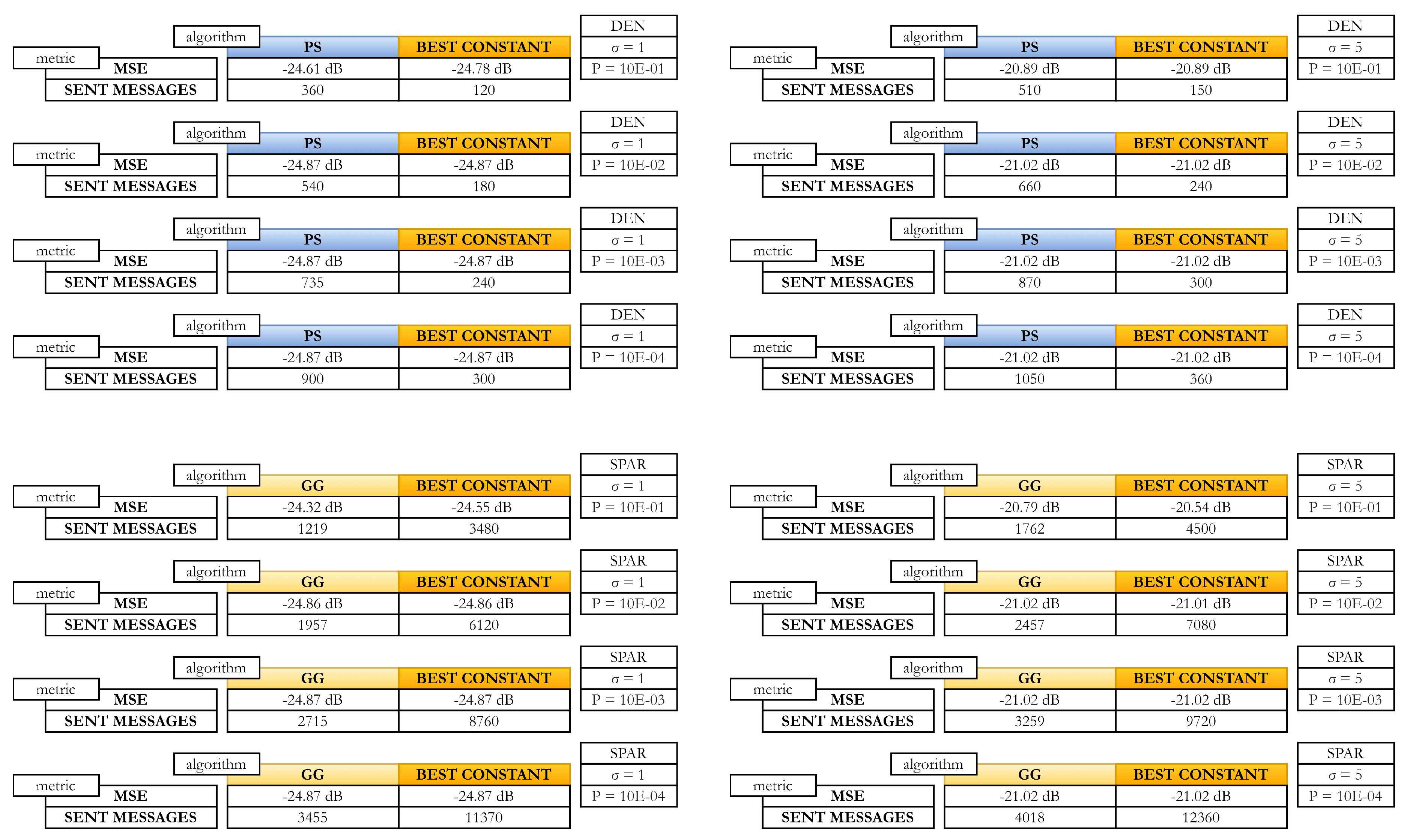
In Figure 18, we compare the best-performing distributed consensus gossip algorithms with the Best Constant weights, a deterministic consensus algorithm recently identified as the top-performing algorithm for suppressing Gaussian noise within its category [65,66]. In densely connected RGGs, the comparison is made with PS, which has been identified as the best gossip algorithm for these graphs. From Figure 18, we can see that the estimation errors of these two algorithms do not notably differ. However, the Best Constant weights requires significantly fewer sent messages than PS in every examined scenario. In sparsely connected RGGs, the Best Constant weights is compared with GG (the best gossip algorithm for these graphs) and achieves nearly the same precision as GG. However, GG significantly outperforms the Best Constant weights in terms of the number of sent messages.
6. Conclusions
The goal of this paper is to examine the applicability of five widely used distributed consensus gossip algorithms for sensor fusion, specifically to suppress incorrect sensor readings represented by Gaussian noise. The algorithms are bounded by a stopping criterion with various initial configurations, tested in RGGs with different connectivity levels, affected by noise with varying values of , and evaluated using two metrics. The presented results show that the best performance is achieved by PS in dense RGGs and by GG in sparse RGGs (indicating that employing geographical routing is beneficial in sparsely connected graphs). All the algorithms, except for BG, achieve very high precision and can significantly alleviate Gaussian noise in WSNs. BG requires the fewest sent messages, but its error is much higher compared to the other algorithms. Although BG can also suppress noise in WSNs, it is not as effective as the other algorithms. MSE of all the algorithms, except for BG, cannot drop below the threshold value determined by (a higher value of causes the value of this threshold to be higher). From the presented results, we can conclude that P = 10E-01 (the highest examined value of P) is the optimal configuration for the applied stopping criterion, as decreasing P has only a marginal or no impact on MSE. However, decreasing P results in an increase in the number of sent messages. Therefore, low values of P offer no benefits compared to error-free scenarios. The most important conclusion is that all the algorithms are effective in suppressing Gaussian noise in WSNs. The algorithms (except on BG) achieve precision similar to that of the best-performing distributed consensus deterministic algorithm (the Best Constant weights). In terms of sent messages, the Best Constant weights algorithm performs better than PS in dense RGGs but is outperformed by GG in sparse RGGs.
Author Contributions
“Conceptualization, M.K. and J.K.; methodology, M.K.; software, M.K.; validation, M.K. and J.K.; formal analysis, M.K. and J.K.; investigation, M.K.; resources, M.K.; data curation, M.K.; writing—original draft preparation, M.K.; writing—review and editing, M.K. and J.K.; visualization, M.K.; supervision, J.K.; project administration, M.K.; funding acquisition, M.K. All authors have read and agreed to the published version of the manuscript.”
Funding
This work was supported by the Slovak Scientific Grant Agency VEGA under the contract 2/0135/23 ”Intelligent sensor systems and data processing” and by the Slovak Research and Development Agency under the contract No. SK-SRB-23-0038 and No. APVV-23-0292.
Institutional Review Board Statement
Not applicable.
Informed Consent Statement
Not applicable.
Data Availability Statement
Not applicable.
Acknowledgments
We would like to thank the anonymous reviewers of this paper for their supportive and insightful comments.
Conflicts of Interest
The authors declare no conflict of interest.
Abbreviations
The following abbreviations are used in this manuscript:
| RG | Randomized Gossip algorithm |
| GG | Geographic Gossip algorithm |
| BG | Broadcast Gossip algorithm |
| PS | Push-Sum protocol |
| PP | Push-Pull protocol |
| WSN | Wireless Sensor Network |
| RGG | Random Geometric Graph |
| IoT | Internet of Things |
| MSE | Mean Square Error |
| IID | Independent and Identically Distributed |
| DEN | Densely connected Random Geometric Graphs |
| SPAR | Sparsely connected Random Geometric Graphs |
| BG 1 | Broadcast Gossip algorithm with = 0.1 |
| BG 2 | Broadcast Gossip algorithm with = 0.5 |
| BG 3 | Broadcast Gossip algorithm with = 0.9 |
| Zigbee | Zonal Intercommunication Global-standard |
| BLE | Bluetooth Low Energy |
| LoRa | Long Range |
| IEEE | Institute of Electrical and Electronics Engineers |
| UAV | Unmanned Aerial Vehicle |
References
- Jamshed, M.A.; Ali, K.; Abbasi, Q.H.; Imran, M.A.; Ur-Rehman, M. Challenges, applications, and future of wireless sensors in Internet of Things: A review. IEEE Sensors Journal 2022, 22, 5482–5494. [Google Scholar] [CrossRef]
- Ouni, R.; Saleem, K. Framework for sustainable wireless sensor network based environmental monitoring. Sustainability 2022, 14, 8356. [Google Scholar] [CrossRef]
- Ahmad, R.; Wazirali, R.; Abu-Ain, T. Machine learning for wireless sensor networks security: An overview of challenges and issues. Sensors 2022, 22, 4730. [Google Scholar] [CrossRef]
- Nakas, C.; Kandris, D.; Visvardis, G. Energy efficient routing in wireless sensor networks: A comprehensive survey. Algorithms 2020, 13, 72. [Google Scholar] [CrossRef]
- Behera, T.M.; Samal, U.C.; Mohapatra, S.K.; Khan, M.S.; Appasani, B.; Bizon, N.; Thounthong, P. Energy-efficient routing protocols for wireless sensor networks: Architectures, strategies, and performance. Electronics 2022, 11, 2282. [Google Scholar] [CrossRef]
- Chen, Shengbo, et al. Indoor temperature monitoring using wireless sensor networks: a SMAC application in smart cities. Sustainable Cities and Society 2020, 61, 102333. [Google Scholar] [CrossRef]
- Vidaña-Vila, E.; Navarro, J.; Borda-Fortuny, C.; Stowell, D.; Alsina-Pagès, R.M. Low-cost distributed acoustic sensor network for real-time urban sound monitoring. Electronics 2020, 9, 2119. [Google Scholar] [CrossRef]
- Metia, S.; Nguyen, H.A.; Ha, Q.P. IoT-enabled wireless sensor networks for air pollution monitoring with extended fractional-order Kalman filtering. Sensors 2021, 21, 5313. [Google Scholar] [CrossRef]
- Mabrouki, J.; Azrour, M.; Dhiba, D.; Farhaoui, Y.; El Hajjaji, S. IoT-based data logger for weather monitoring using arduino-based wireless sensor networks with remote graphical application and alerts. Big Data Mining and Analytics 2021, 4, 25–32. [Google Scholar] [CrossRef]
- Aminian, M.; Naji, H.R. A hospital healthcare monitoring system using wireless sensor networks. J. Health Med. Inform 2013, 4, 121. [Google Scholar] [CrossRef]
- Nourildean, S.W.; Hassib, M.D.; Mohammed, Y.A. Internet of things based wireless sensor network: a review. Indones. J. Electr. Eng. Comput. Sci 2022, 27, 246–261. [Google Scholar] [CrossRef]
- Ragnoli, M.; Leoni, A.; Barile, G.; Ferri, G.; Stornelli, V. LoRa-Based Wireless Sensors Network for Rockfall and Landslide Monitoring: A Case Study in Pantelleria Island with Portable LoRaWAN Access. J. Low Power Electron. Appl. 2022, 12, 47. [Google Scholar] [CrossRef]
- Labib, M.I.; ElGazzar, M.; Ghalwash, A.; AbdulKader, S.N. An efficient networking solution for extending and controlling wireless sensor networks using low-energy technologies. PeerJ Computer Science 2021, 7, e780. [Google Scholar] [CrossRef] [PubMed]
- Suji Prasad, S.J. , et al. An efficient LoRa-based smart agriculture management and monitoring system using wireless sensor networks. International Journal of Ambient Energy 2022, 43, 5447–5450. [Google Scholar] [CrossRef]
- Akbar, M.S.; Hussain, Z.; Sheng, M.; Shankaran, R. Wireless body area sensor networks: Survey of mac and routing protocols for patient monitoring under IEEE 802.15.4 and IEEE 802.15.6. Sensors 2022, 22, 8279. [Google Scholar] [CrossRef]
- Malik, N.N.; Alosaimi, W.; Uddin, M.I.; Alouffi, B.; Alyami, H. Wireless sensor network applications in healthcare and precision agriculture. Journal of Healthcare Engineering 2020, 1, 8836613. [Google Scholar] [CrossRef]
- Huanan, Z.; Suping, X.; Jiannan, W. Security and application of wireless sensor network. Procedia Computer Science 2021, 183, 486–492. [Google Scholar] [CrossRef]
- Ullo, S.L.; Sinha, G.R. Advances in smart environment monitoring systems using IoT and sensors. Sensors 2020, 20, 3113. [Google Scholar] [CrossRef]
- Majid, M.; Habib, S.; Javed, A.R.; Rizwan, M.; Srivastava, G.; Gadekallu, T.R.; Lin, J.C.W. Applications of wireless sensor networks and internet of things frameworks in the industry revolution 4.0: A systematic literature review. Sensors 2022, 22, 2087. [Google Scholar] [CrossRef] [PubMed]
- Dampage, U.; Bandaranayake, L.; Wanasinghe, R.; Kottahachchi, K.; Jayasanka, B. Forest fire detection system using wireless sensor networks and machine learning. Scientific reports 2022, 12, 46. [Google Scholar] [CrossRef]
- Arshad, Jehangir, et al. Deployment of wireless sensor network and iot platform to implement an intelligent animal monitoring system. Sustainability 2022, 14, 6249. [Google Scholar] [CrossRef]
- Ragnoli, M.; Barile, G.; Leoni, A.; Ferri, G.; Stornelli, V. An autonomous low-power LoRa-based flood-monitoring system. Journal of Low Power Electronics and Applications 2020, 10, 15. [Google Scholar] [CrossRef]
- Abdollahi, A.; Rejeb, K.; Rejeb, A.; Mostafa, M.M.; Zailani, S. Wireless sensor networks in agriculture: Insights from bibliometric analysis. Sustainability 2021, 13, 12011. [Google Scholar] [CrossRef]
- Haque, M.E.; Asikuzzaman, M.; Khan, I.U.; Ra, I.H.; Hossain, M.S.; Shah, S.B.H. Comparative study of IoT-based topology maintenance protocol in a wireless sensor network for structural health monitoring. Remote sensing 2020, 12, 2358. [Google Scholar] [CrossRef]
- Ezeigweneme, C.A.; Nwasike, C.N.; Adekoya, O.O.; Biu, P.W.; Gidiagba, J.O. Wireless communication in electro-mechanical systems: investigating the rise and implications of cordless interfaces for system enhancement. Engineering Science and Technology Journal 2024, 5, 21–42. [Google Scholar] [CrossRef]
- Sungheetha, A.; Sharma, R. Real time monitoring and fire detection using internet of things and cloud based drones. Journal of Soft Computing Paradigm 2020, 2, 168–174. [Google Scholar] [CrossRef]
- Amutha, J.; Sharma, S.; Nagar, J. WSN strategies based on sensors, deployment, sensing models, coverage and energy efficiency: Review, approaches and open issues. Wireless Personal Communications 2020, 111, 1089–1115. [Google Scholar] [CrossRef]
- Sigrist, L.; Ahmed, R.; Gomez, A.; Thiele, L. Harvesting-aware optimal communication scheme for infrastructure-less sensing. ACM Transactions on Internet of Things 2020, 1, 1–26. [Google Scholar] [CrossRef]
- Alghamdi, T.A. Energy efficient protocol in wireless sensor network: optimized cluster head selection model. Telecommunication Systems 2020, 74, 331–345. [Google Scholar] [CrossRef]
- Yun, W.K.; Yoo, S.J. Q-learning-based data-aggregation-aware energy-efficient routing protocol for wireless sensor networks. IEEE Access 2021, 9, 10737–10750. [Google Scholar] [CrossRef]
- Sachan, S.; Sharma, R.; Sehgal, A. Energy efficient scheme for better connectivity in sustainable mobile wireless sensor networks. Sustainable Computing: Informatics and Systems 2021, 30, 100504. [Google Scholar] [CrossRef]
- Landaluce, H.; Arjona, L.; Perallos, A.; Falcone, F.; Angulo, I.; Muralter, F. A review of IoT sensing applications and challenges using RFID and wireless sensor networks. Sensors 2020, 20, 2495. [Google Scholar] [CrossRef] [PubMed]
- Dobrescu, R.; Popescu, D.; Nicolae, M.; Mocanu, S. Hybrid wireless sensor network for homecare monitoring of chronic patients. International journal of biology and biomedical engineering 2009, 3, 19–26. [Google Scholar]
- Lata, S; , Mehfuz, S. ; Urooj, S.; Alrowais, F. Fuzzy clustering algorithm for enhancing reliability and network lifetime of wireless sensor networks. IEEE Access 2020, 8, 66013–66024. [Google Scholar] [CrossRef]
- Ahmad, R.; Wazirali, R.; Abu-Ain, T. Machine learning for wireless sensor networks security: An overview of challenges and issues. Sensors 2022, 22, 4730. [Google Scholar] [CrossRef] [PubMed]
- Chamam, A.; Pierre, S. On the planning of wireless sensor networks: Energy-efficient clustering under the joint routing and coverage constraint. IEEE Transactions on Mobile Computing 2009, 8, 1077–1086. [Google Scholar] [CrossRef]
- Buratti, C.; Conti, A.; Dardari, D.; Verdone, R. An overview on wireless sensor networks technology and evolution. Sensors 2009, 9, 6869–6896. [Google Scholar] [CrossRef] [PubMed]
- Izadi, D.; Abawajy, J.H.; Ghanavati, S.; Herawan, T. A data fusion method in wireless sensor networks. Sensors 2015, 15, 2964–297. [Google Scholar] [CrossRef] [PubMed]
- Bissadu, K.D.; Hossain, G.; Velagala, L.P. Identifying Sensors Data Integrity Threats of Smart Agriculture: A Collaborative Filtering Approach. Applied Engineering in Agriculture 2024, 40, 565–575. [Google Scholar] [CrossRef]
- Bonnet, P.; Gehrke, J.; Seshadri, P. Towards sensor database systems. Lecture Notes in Computer Science 2001, 1987, 3–14. [Google Scholar]
- Pirayesh, H.; Zeng, H. Jamming attacks and anti-jamming strategies in wireless networks: A comprehensive survey. IEEE communications surveys 2022, 24, 767–809. [Google Scholar] [CrossRef]
- Kavousi-Fard, A.; Su, W.; Jin, T. A machine-learning-based cyber attack detection model for wireless sensor networks in microgrids. IEEE Transactions on Industrial Informatics 2020, 17, 650–658. [Google Scholar] [CrossRef]
- Krishnamurthi, R; , Kumar, A. ; Gopinathan, D.; Nayyar, A.; Qureshi, B. An overview of IoT sensor data processing, fusion, and analysis techniques. Sensors 2020, 20, 6076. [Google Scholar] [CrossRef] [PubMed]
- Yeong, D.J.; Velasco-Hernandez, G.; Barry, J.; Walsh, J. Sensor and sensor fusion technology in autonomous vehicles: A review. Sensors 2021, 21, 2140. [Google Scholar] [CrossRef]
- Wei, Y.; Wu, D.; Terpenny, J. Robust incipient fault detection of complex systems using data fusion. IEEE Transactions on Instrumentation and Measurement 2020, 69, 9526–9534. [Google Scholar] [CrossRef]
- Kong, L.; Peng, X.; Chen, Y.; Wang, P.; Xu, M. Multi-sensor measurement and data fusion technology for manufacturing process monitoring: a literature review. International journal of extreme manufacturing 2020, 2, 022001. [Google Scholar] [CrossRef]
- Li, D.; Wang, Y.; Wang, J.; Wang, C.; Duan, Y. Recent advances in sensor fault diagnosis: A review. Sensors and Actuators A: Physical 2020, 309, 111990. [Google Scholar] [CrossRef]
- Saeedi, I.D.I.; Al-Qurabat, A.K.M. A systematic review of data aggregation techniques in wireless sensor networks. Journal of Physics: Conference Series 2021, 1818, 012194. [Google Scholar]
- Xiao, L.; Boyd, S.; Lall, S. A scheme for robust distributed sensor fusion based on average consensus. In Proceedings of the IPSN 2005. Fourth International Symposium on Information Processing in Sensor Networks, Boise, ID, USA, 15-15 April 2005; p. 63. [Google Scholar]
- Shrimali, B.; Patel, H.B. Blockchain state-of-the-art: architecture, use cases, consensus, challenges and opportunities. Journal of King Saud University-Computer and Information Sciences 2022, 34, 6793–6807. [Google Scholar] [CrossRef]
- Mostefaoui, A.; Raynal, M. Leader-based consensus. Parallel Processing Letters 2001, 11, 95–107. [Google Scholar] [CrossRef]
- Merezeanu, D.; Nicolae, M. Consensus control of discrete-time multi-agent systems. Univ. Politeh. Buchar. Ser. A 2017, 79, 167–174. [Google Scholar]
- Stamatescu, G.; Stamatescu, I.; Popescu, D. Consensus-based data aggregation for wireless sensor networks. Journal of Control Engineering and Applied Informatics 2017, 19, 43–50. [Google Scholar]
- Dragana, C.; Mihai, V.; Stamatescu, G.; Popescu, D. In-network stochastic consensus for WSN surveillance applications. In Proceedings of the 9th International Conference on Electronics, Computers and Artificial Intelligence, ECAI 2017, Targoviste, Romania, 29 June 2017-01 July 2017; p. 1. [Google Scholar]
- Lizzio, F.F.; Capello, E.; Guglieri, G. A review of consensus-based multi-agent UAV implementations. Journal of Intelligent and Robotic Systems 2022, 106, 43. [Google Scholar] [CrossRef]
- Sharma, A.B.; Golubchik, L.; Govindan, R. Sensor faults: Detection methods and prevalence in real-world datasets. ACM Transactions on Sensor Networks (TOSN) 2010, 6, 1–39. [Google Scholar] [CrossRef]
- Clegg, M.; Marzullo, K. Predicting physical processes in the presence of faulty sensor readings. Proceedings of IEEE 27th International Symposium on Fault Tolerant Computing, Seattle, WA, USA, 24-27 June 1997; pp. 373–378. [Google Scholar]
- Elnahrawy, E.; Nath, B. Cleaning and querying noisy sensors. In Proceedings of the 2nd ACM international conference on Wireless sensor networks and applications, New York, NY, USA, 19 September 2003; p. 78. [Google Scholar]
- Chen, Y.; Jiang, S.; Yang, J.; Song, K.; Wang, Q. Grey bootstrap method for data validation and dynamic uncertainty estimation of self-validating multifunctional sensors. Chemometrics and Intelligent Laboratory Systems 2015, 146, 63–76. [Google Scholar] [CrossRef]
- Yu, Y.; Li, H. Virtual in-situ calibration method in building systems. Automation in Construction 2015, 59, 59–67. [Google Scholar] [CrossRef]
- Solomakhina, N.; Hubauer, T.; Lamparter, S.; Roshchin, M.; Grimm, S. Extending statistical data quality improvement with explicit domain models. Proceedings of 2014 12th IEEE International Conference on Industrial Informatics (INDIN), Porto Alegre, Brazil, 27-30 July 2014; pp. 720–725. [Google Scholar]
- Scheffel, R.M.; Fröhlich, A.A. Increasing sensor reliability through confidence attribution. Journal of the Brazilian Computer Society 2019, 25, 13. [Google Scholar] [CrossRef]
- Sinha, A.; Das, D. SNRepair: systematically addressing sensor faults and self-calibration in IoT networks. IEEE Sensors Journal 2023, 23, 14915–14922. [Google Scholar] [CrossRef]
- Ayanoglu, M.B.; Uysal, I. ML Approach to Improve the Costs and Reliability of a Wireless Sensor Network. Sensors 2023, 23, 4303. [Google Scholar] [CrossRef] [PubMed]
- Kenyeres, M.; Kenyeres, J. Average Consensus with Perron Matrix for Alleviating Inaccurate Sensor Readings Caused by Gaussian Noise in Wireless Sensor Networks. Lecture Notes in Networks and Systems 2021, 230, 391–405. [Google Scholar]
- Kenyeres, M.; Kenyeres, J. Using Metropolis-Hastings Algorithm with Stopping Criterion to Suppress Incorrect Sensor Data. Lecture Notes in Networks and Systems.
- Fraser, B.; Coyle, A.; Hunjet, R.; Szabo, C. An Analytic Latency Model for a Next-Hop Data-Ferrying Swarm on Random Geometric Graphs. IEEE Access 2020, 8, 48929–48942. [Google Scholar] [CrossRef]
- Gulzar, M.M.; Rizvi, S.T.H.; Javed, M.Y.; Munir, U.; Asif, H. Multi-agent cooperative control consensus: A comparative review. Electronics 2018, 7, 22. [Google Scholar] [CrossRef]
- Bonato, A.; Lozier, M.; Mitsche, D.; Pérez-Giménez, X.; Prałat, P. The domination number of on-line social networks and random geometric graphs. In Theory and Applications of Models of Computation: 12th Annual Conference, TAMC 2015, Location of Conference, Singapore, 18-; pp. 150–163. 20 May.
- Kenniche, H.; Ravelomananana, V. Random geometric graphs as model of wireless sensor networks. Proceedings of 2010 The 2nd International Conference on Computer and Automation Engineering (ICCAE), Singapur, 26-28 February 2010; pp. 103–107. [Google Scholar]
- Meng, J.; Li, H.; Han, Z. Sparse event detection in wireless sensor networks using compressive sensing. Proceedings of 2009 43rd Annual Conference on Information Sciences and Systems, Baltimore, MD, USA, 18-20 March 2009; pp. 181–185. [Google Scholar]
- Banos, O.; Damas, M.; Pomares, H.; Rojas, I. On the use of sensor fusion to reduce the impact of rotational and additive noise in human activity recognition. Sensors 2012, 12, 8039–8054. [Google Scholar] [CrossRef]
- Kenyeres, M.; Kenyeres, J. Comparative Study of Distributed Consensus Gossip Algorithms for Network Size Estimation in Multi-Agent Systems. Future Internet 2021, 13, 134. [Google Scholar] [CrossRef]
- Gutierrez-Gutierrez, J.; Zarraga-Rodriguez, M.; Insausti, X. Analysis of Known Linear Distributed Average Consensus Algorithms on Cycles and Paths. Sensors 2018, 18, 968. [Google Scholar] [CrossRef] [PubMed]
- Dimakis, A.A.G.; Sarwate, A.D.; Wainwright, M.J.; Scaglione, A. Geographic gossip: Efficient averaging for sensor networks. IEEE Trans. Signal Process. 2008, 56, 1205–1216. [Google Scholar] [CrossRef]
- Aysal, T.C.; Yildiz, M.E.; Sarwate, A.D.; Scaglione, A. Broadcast gossip algorithms for consensus. IEEE Trans. Signal Process. 2009, 57, 2748–2761. [Google Scholar] [CrossRef]
- Kempe, D.; Dobra, A.; Gehrke, J. Gossip-based computation of aggregate information. In Proceedings of the 44th Annual IEEE Symposium on Foundations of Computer Science, FOCS 2003, Cambridge, MA, USA, 11–14 October 2003; pp. 482–491. [Google Scholar]
- Jelasity, M.; Montresor, A.; Babaoglu, O. Gossip-based aggregation in large dynamic networks. ACM Transactions on Computer Systems (TOCS). 2005, 23, 219–252. [Google Scholar] [CrossRef]
- Skorpil, V.; Stastny, J. Back-propagation and k-means algorithms comparison. In Proceedings of the 2006 8th International Conference on Signal Processing, ICSP 2006, Guilin, China, 16–20 November 2006; pp. 374–378. [Google Scholar]
- Lee, C.S.; Michelusi, N.; Scutari, G. Finite rate distributed weight-balancing and average consensus over digraphs. IEEE Transactions on Automatic Control 2020, 66, 4530–4545. [Google Scholar] [CrossRef]
Figure 1.
Typical architecture of sensor node in wireless sensor networks.
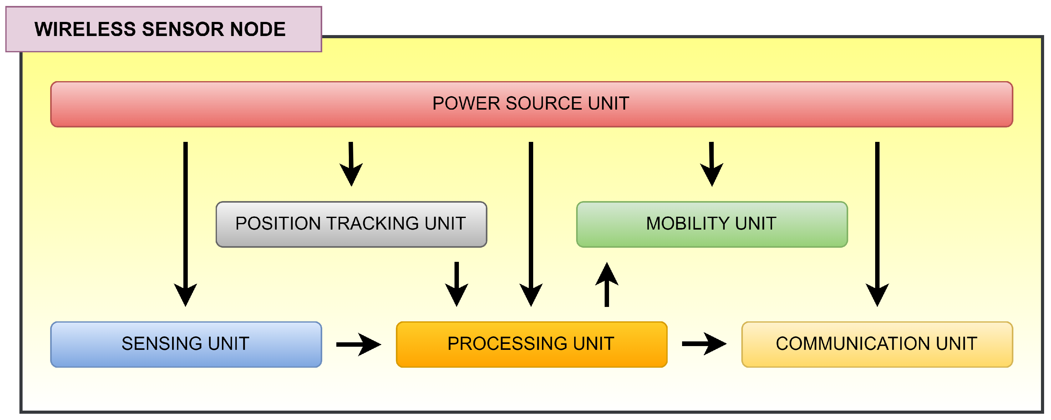
Figure 2.
Typical architecture of wireless sensor networks.
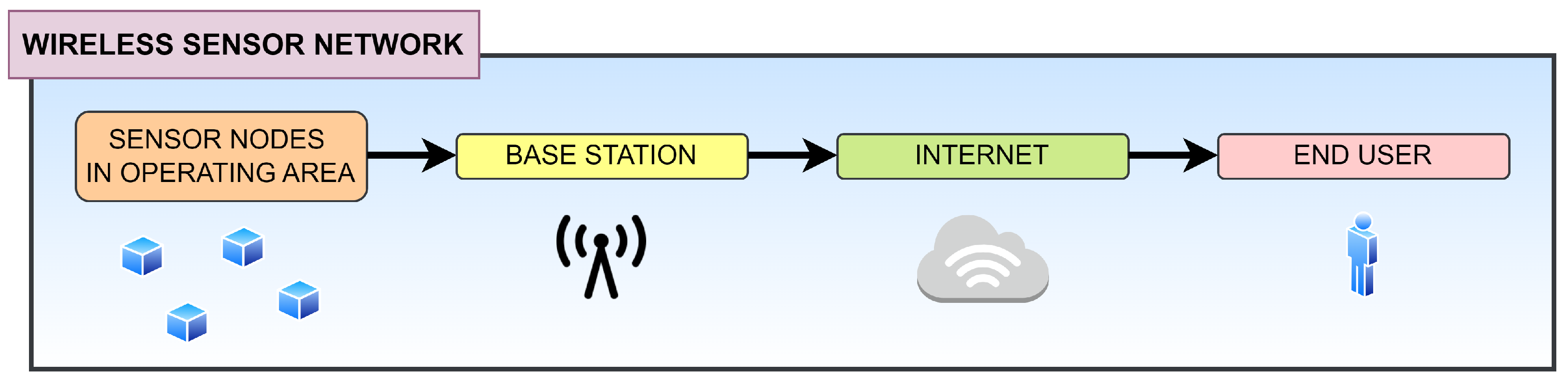
Figure 3.
General architecture of sensor fusion in wireless sensor networks.
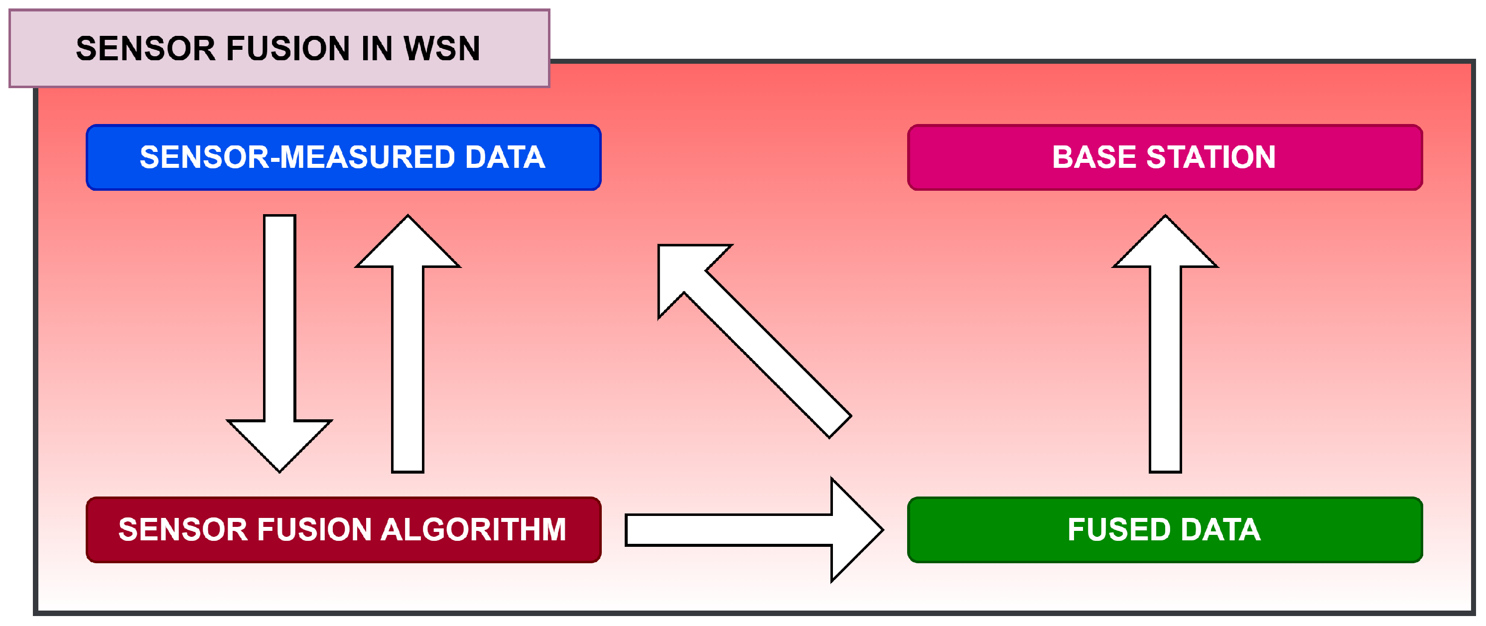
Figure 4.
Example of incorrect sensor readings in wireless sensor networks.
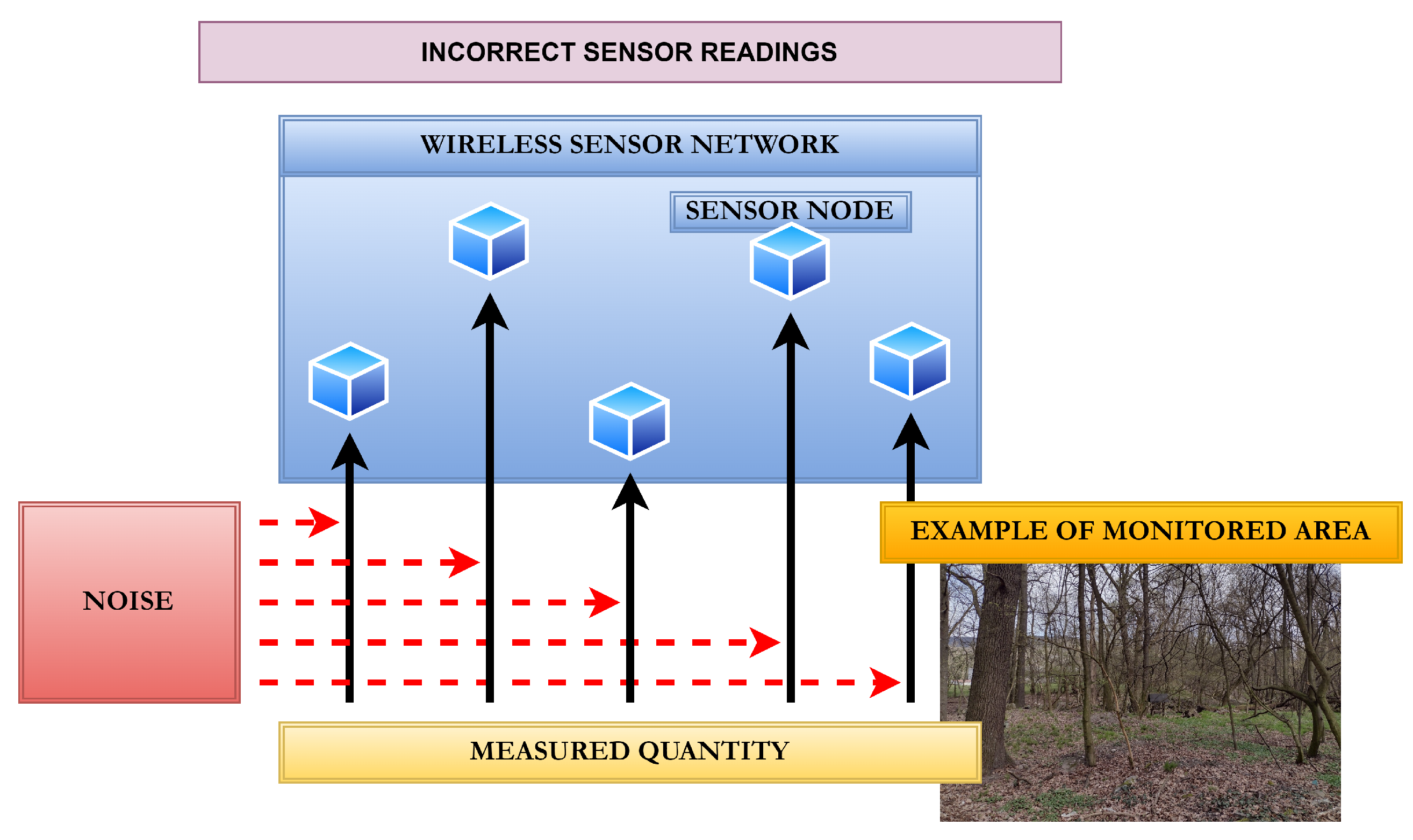
Figure 5.
Example of undirected, simple, finite, connected graph.
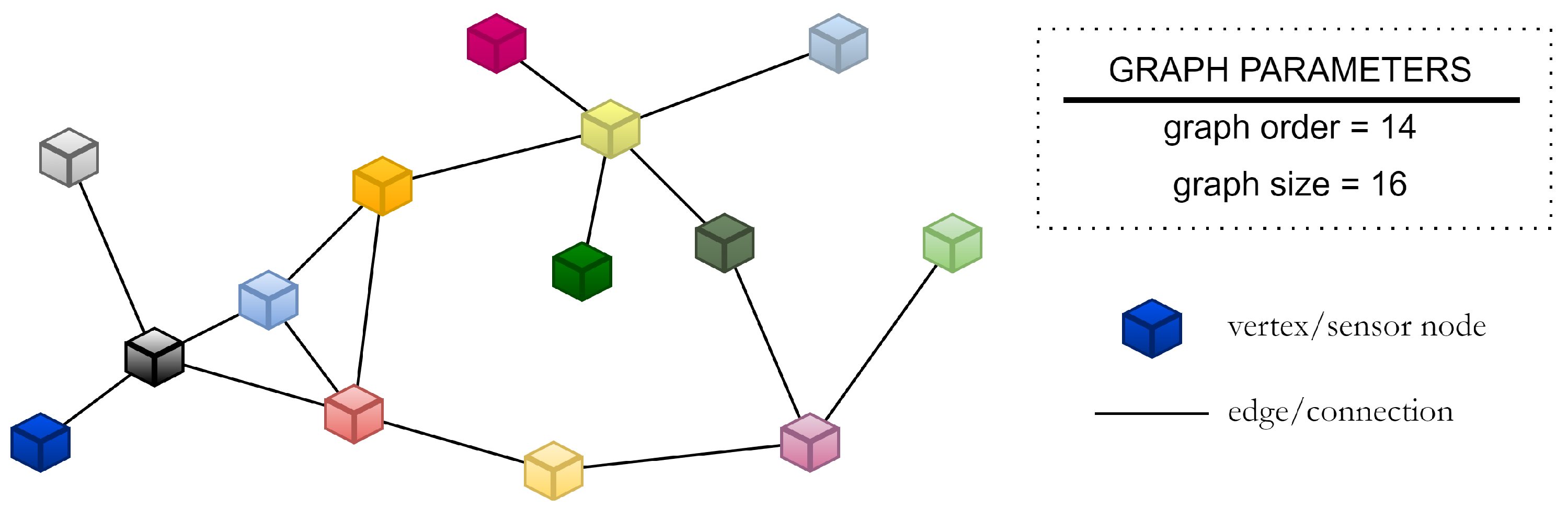
Figure 6.
Example of how distributed consensus gossip algorithms can suppress Gaussian noise—left figure: no sensor fusion is applied; right figure: sensor fusion (Randomized Gossip) is applied.
Figure 6.
Example of how distributed consensus gossip algorithms can suppress Gaussian noise—left figure: no sensor fusion is applied; right figure: sensor fusion (Randomized Gossip) is applied.
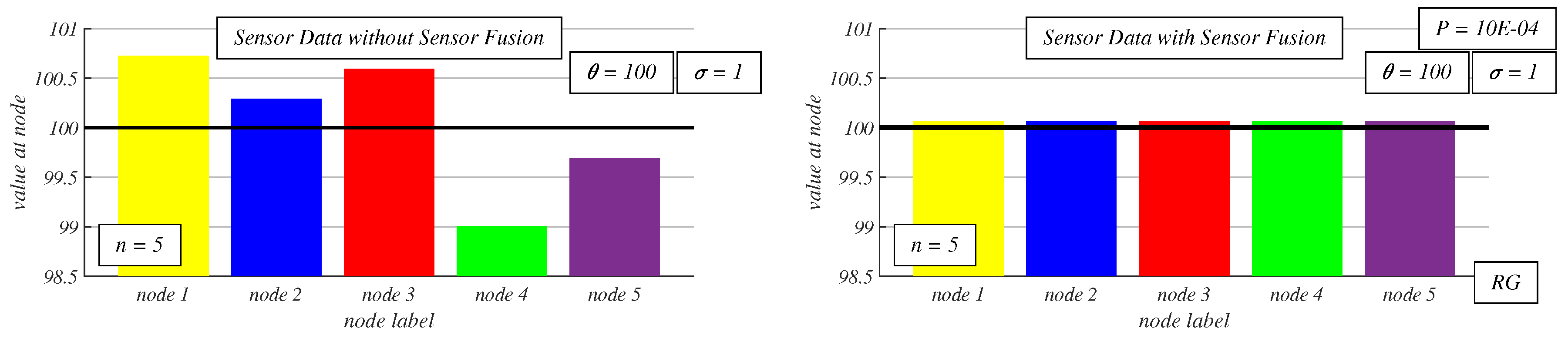
Figure 7.
Evolution of inner states when data are skewed due to Gaussian noise (Randomized Gossip is applied).
Figure 7.
Evolution of inner states when data are skewed due to Gaussian noise (Randomized Gossip is applied).
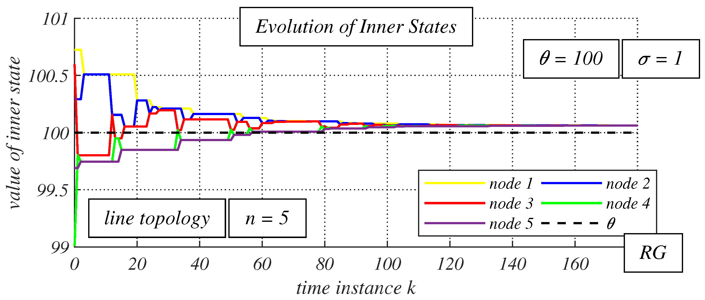
Figure 8.
Example of how value of P affects estimation error and number of sent messages.
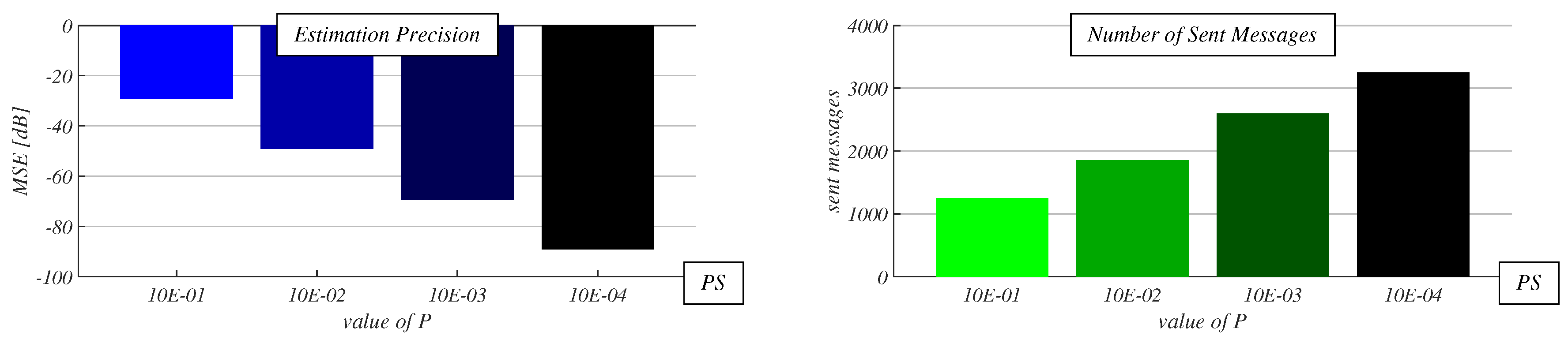
Figure 9.
Example of densely connected (left figure) and sparsely connected (right figure) random geometric graphs with n = 30.
Figure 9.
Example of densely connected (left figure) and sparsely connected (right figure) random geometric graphs with n = 30.
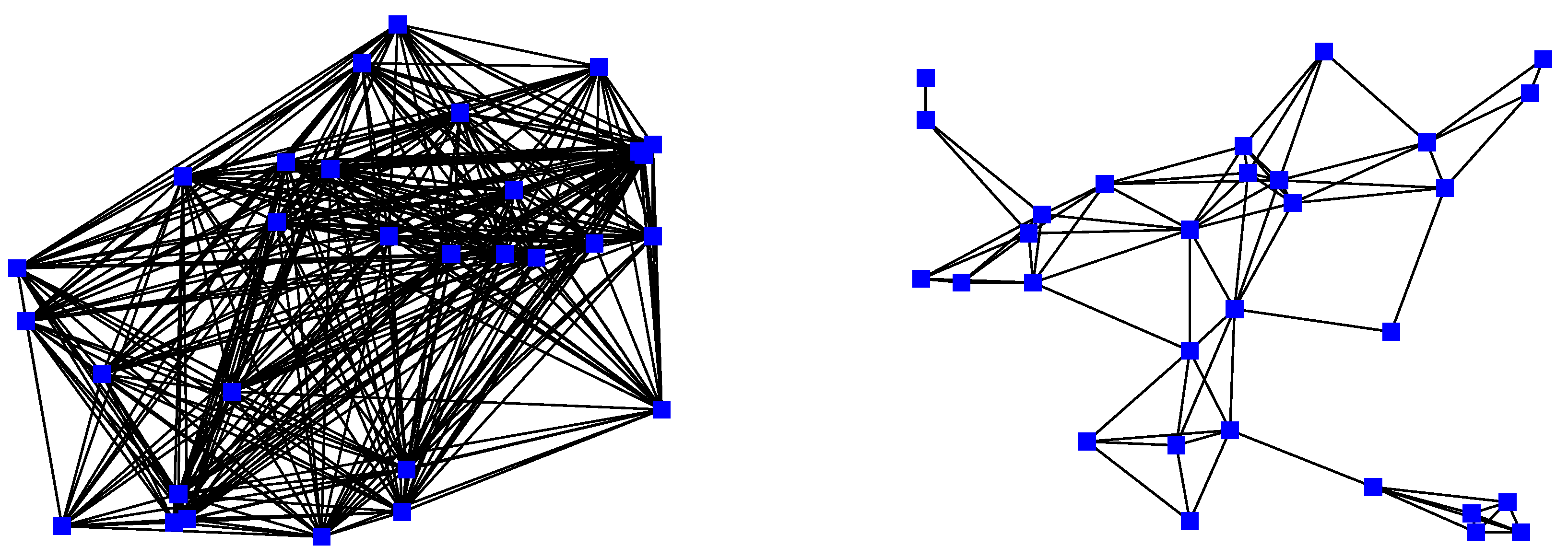
Figure 10.
Mean square error for various precisions of applied stopping criterion, in dense random geometric graphs, and for = 1.
Figure 10.
Mean square error for various precisions of applied stopping criterion, in dense random geometric graphs, and for = 1.
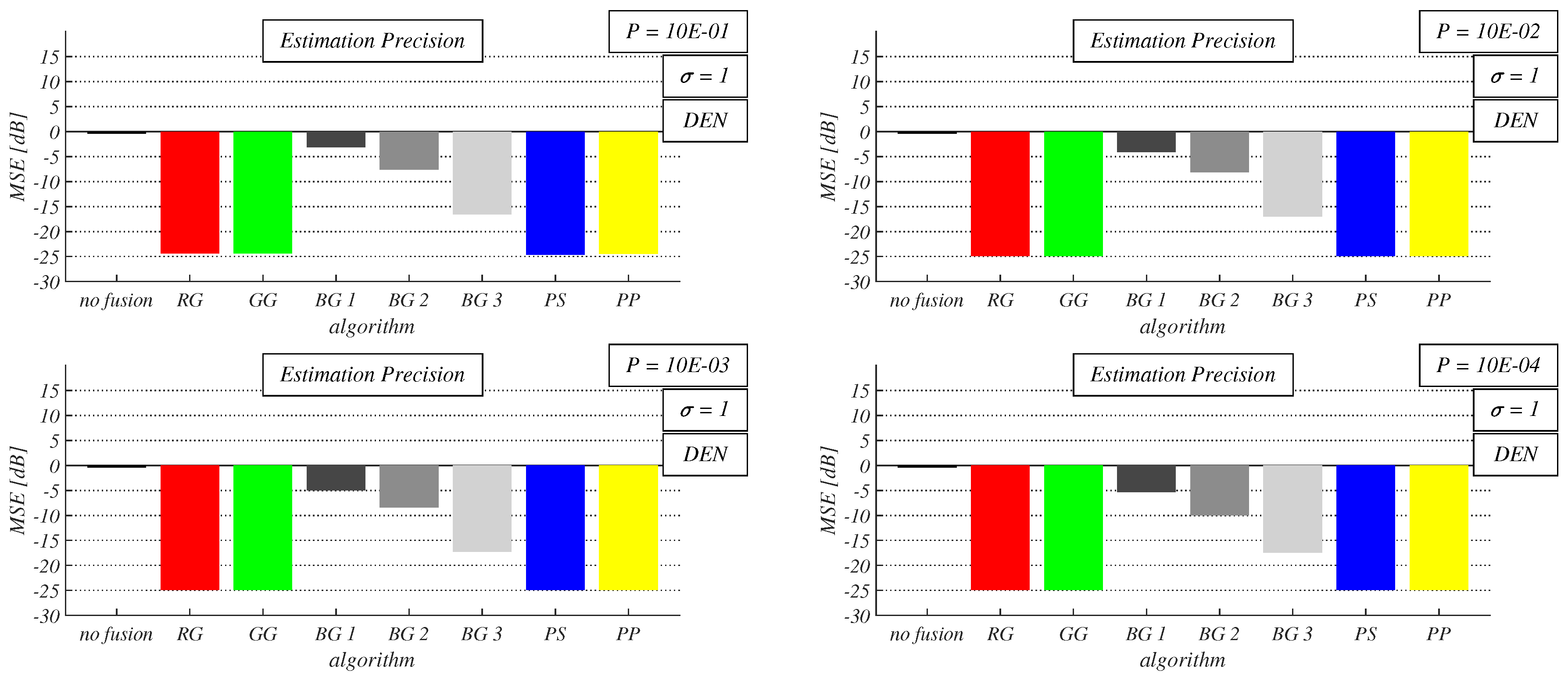
Figure 11.
Mean square error for various precisions of applied stopping criterion, in sparse random geometric graphs, and for = 1.
Figure 11.
Mean square error for various precisions of applied stopping criterion, in sparse random geometric graphs, and for = 1.
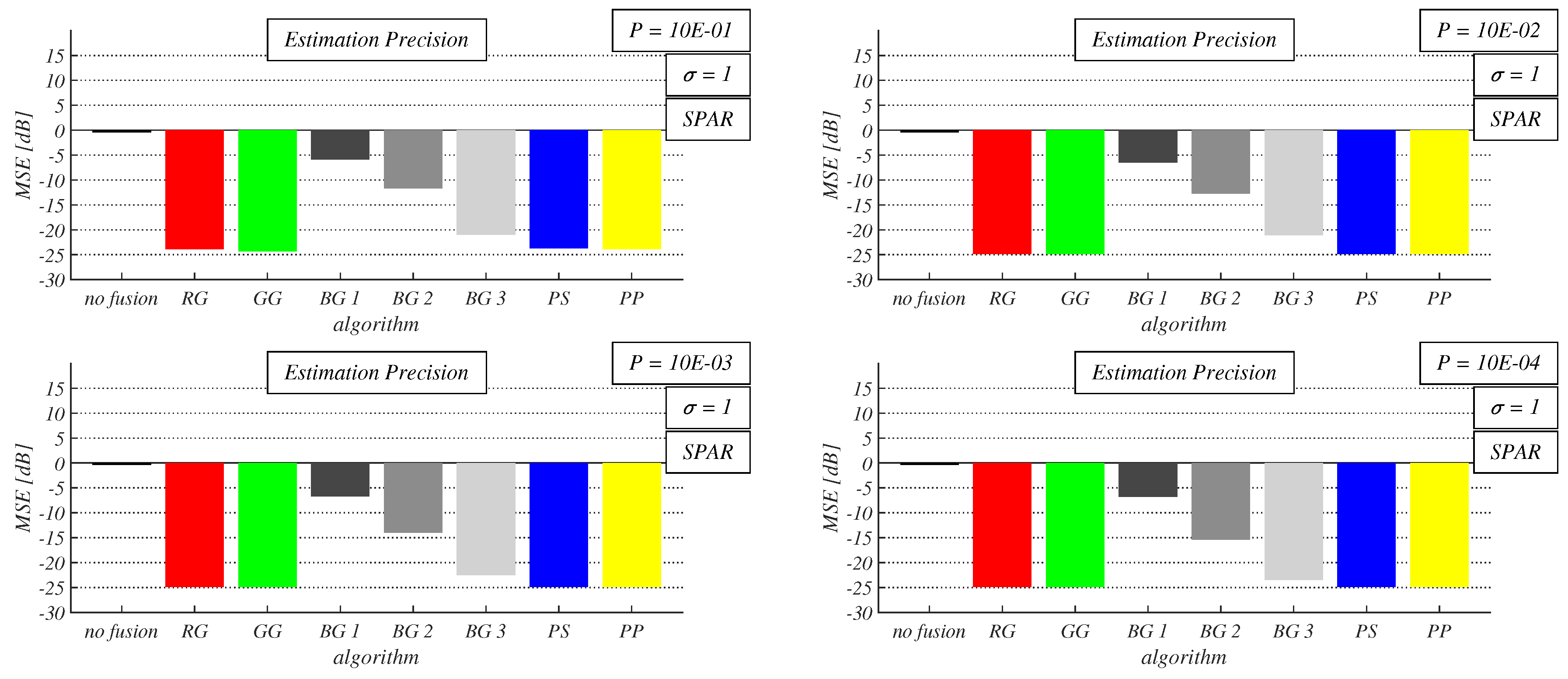
Figure 12.
Mean square error for various precisions of applied stopping criterion, in dense random geometric graphs, and for = 5.
Figure 12.
Mean square error for various precisions of applied stopping criterion, in dense random geometric graphs, and for = 5.
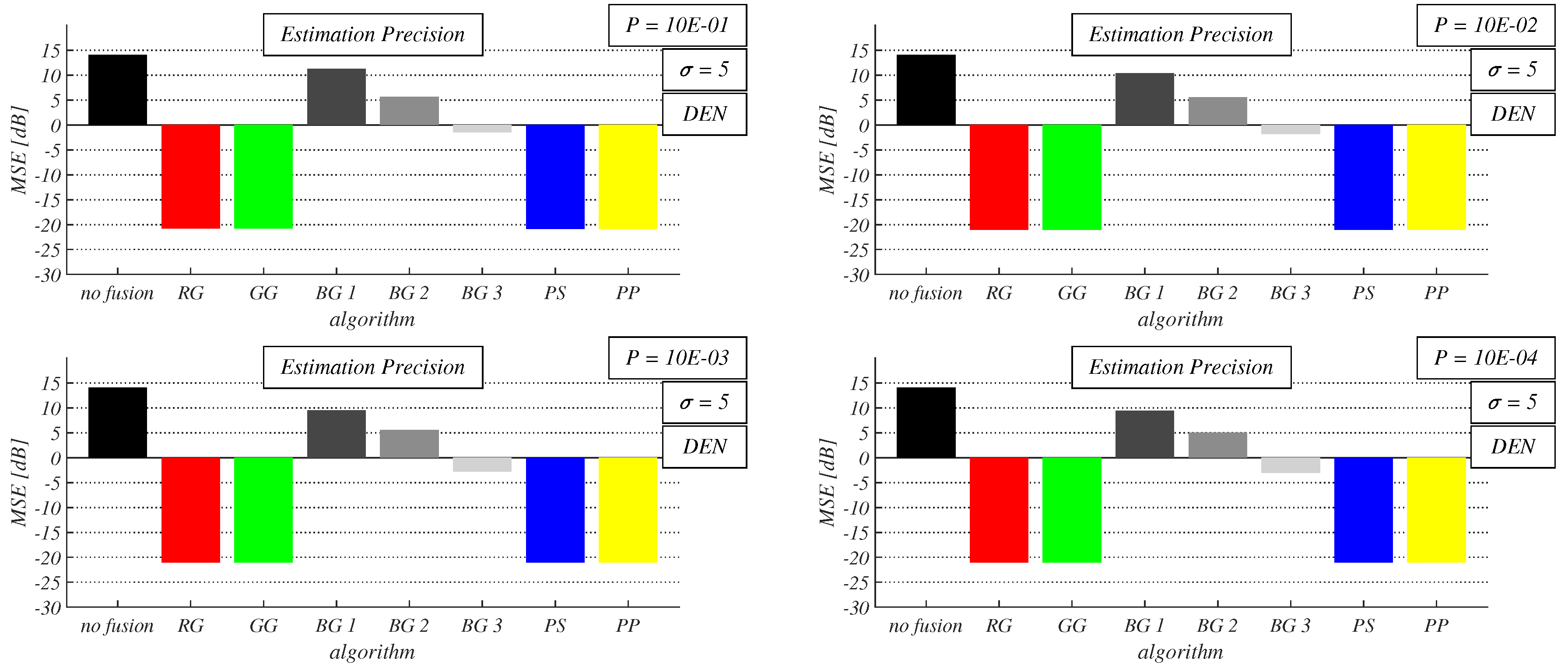
Figure 13.
Mean square error for various precisions of applied stopping criterion, in sparse random geometric graphs, and for = 5.
Figure 13.
Mean square error for various precisions of applied stopping criterion, in sparse random geometric graphs, and for = 5.
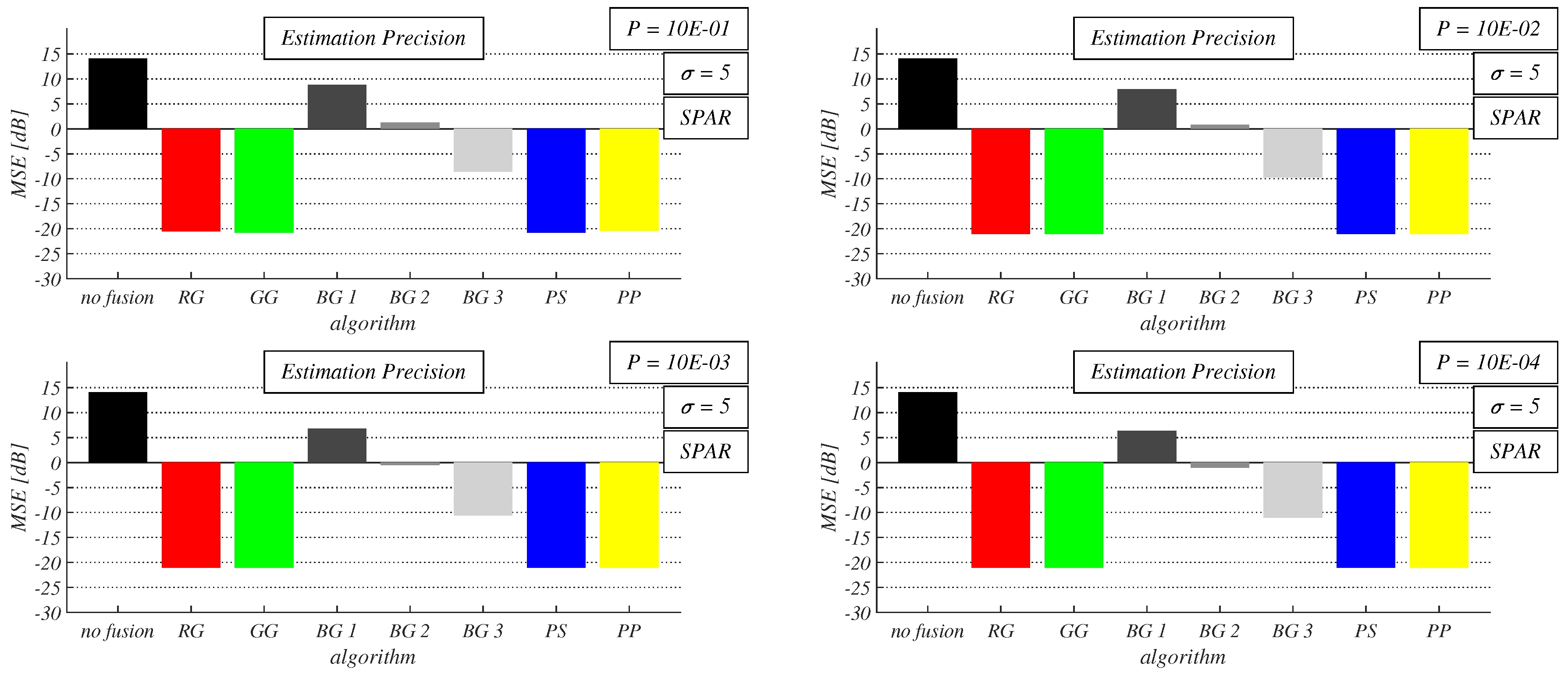
Figure 14.
Number of sent messages for various precisions of applied stopping criterion, in dense random geometric graphs, and for = 1.
Figure 14.
Number of sent messages for various precisions of applied stopping criterion, in dense random geometric graphs, and for = 1.
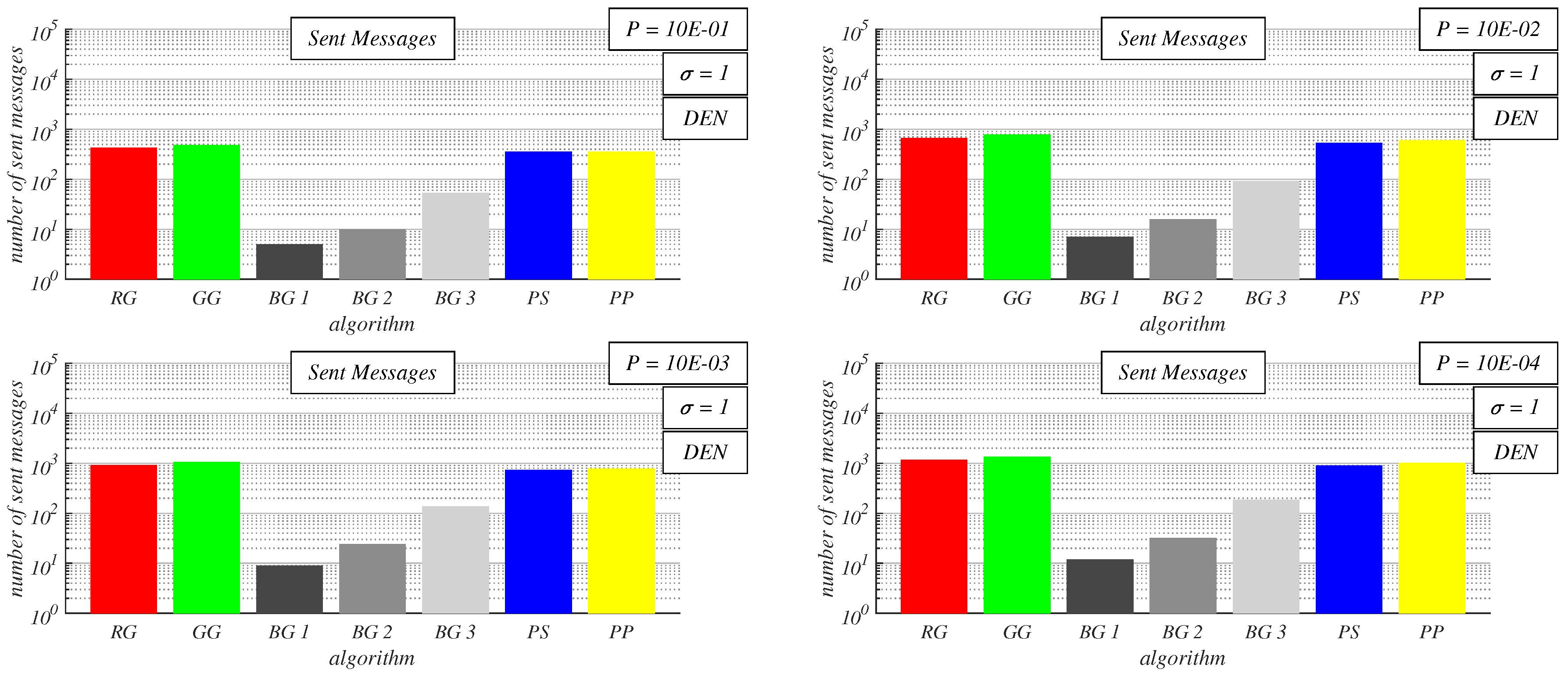
Figure 15.
Number of sent messages for various precisions of applied stopping criterion, in sparse random geometric graphs, and for = 1.
Figure 15.
Number of sent messages for various precisions of applied stopping criterion, in sparse random geometric graphs, and for = 1.
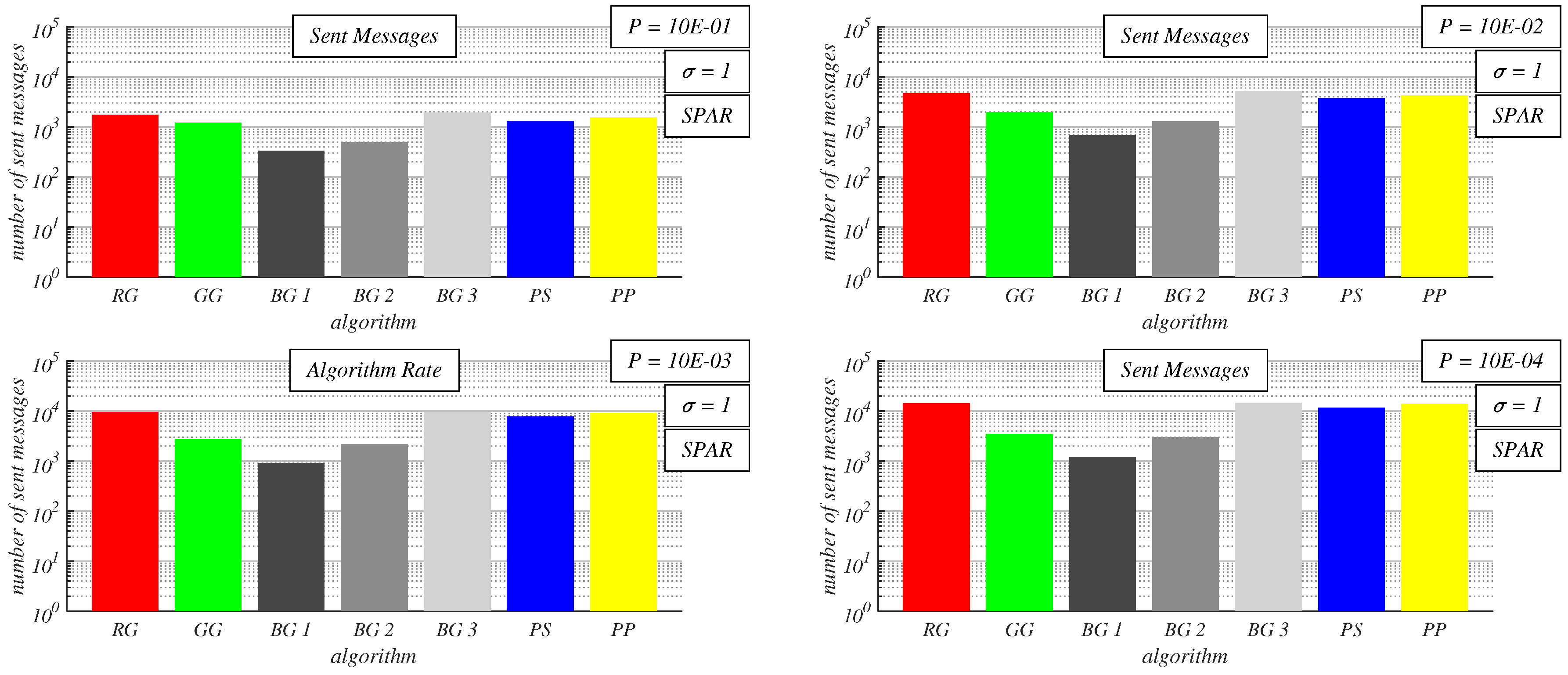
Figure 16.
Number of sent messages for various precisions of applied stopping criterion, in dense random geometric graphs, and for = 5.
Figure 16.
Number of sent messages for various precisions of applied stopping criterion, in dense random geometric graphs, and for = 5.
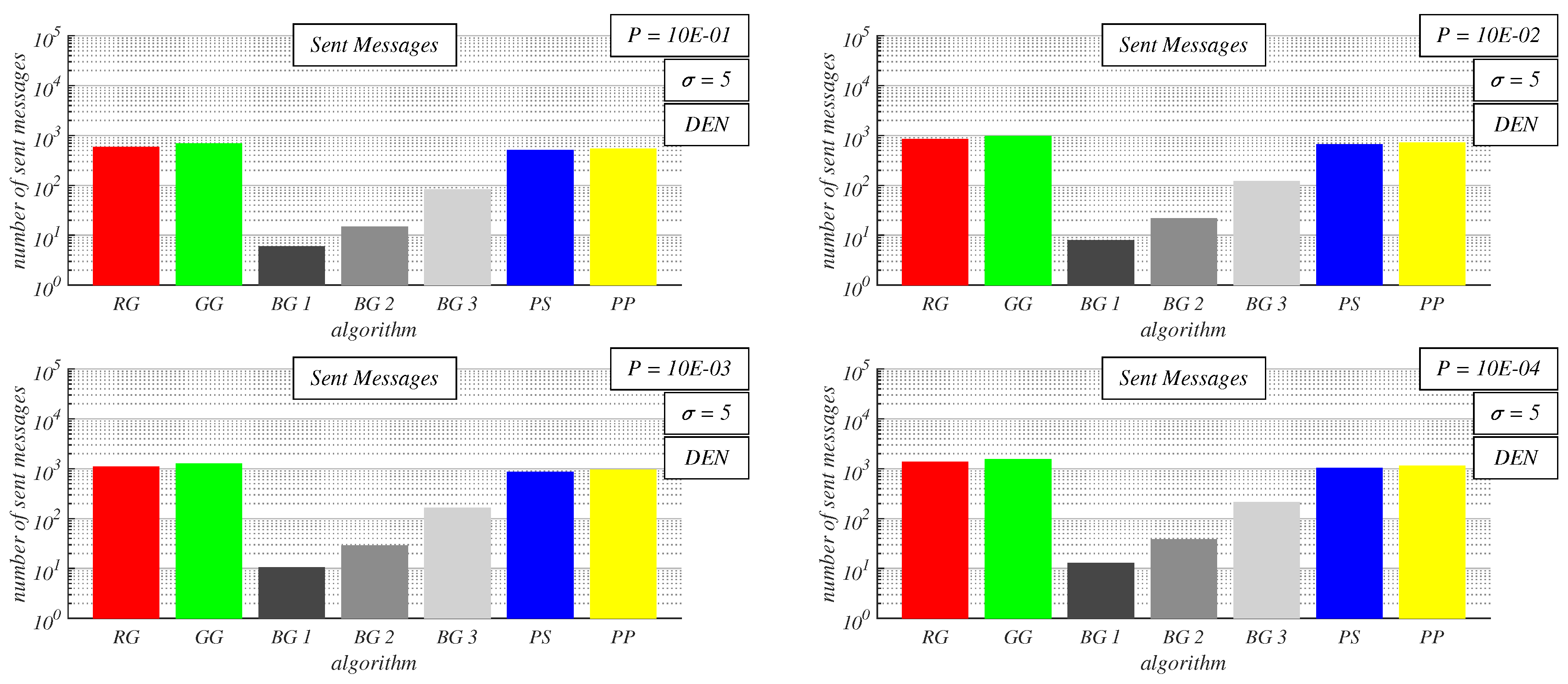
Figure 17.
Number of sent messages for various precisions of applied stopping criterion, in sparse random geometric graphs, and for = 5.
Figure 17.
Number of sent messages for various precisions of applied stopping criterion, in sparse random geometric graphs, and for = 5.
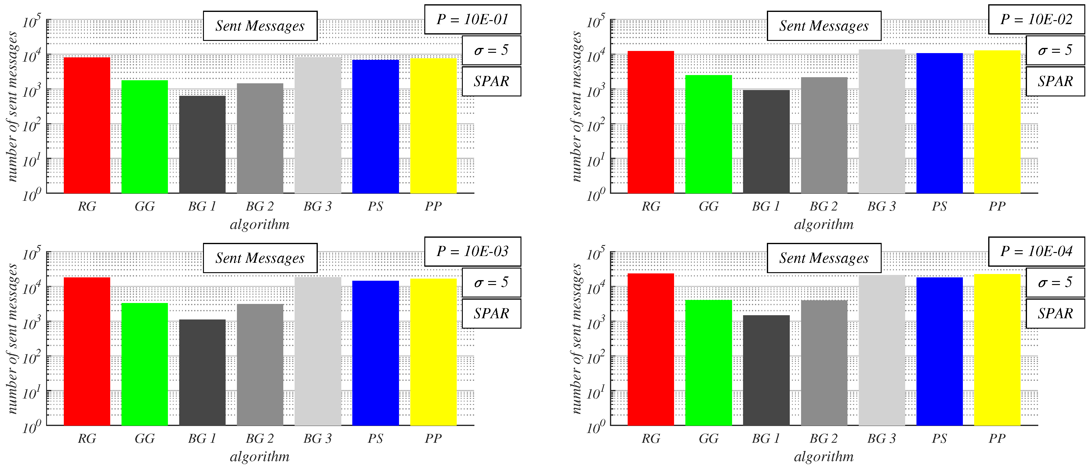
Figure 18.
Comparison of best-performing gossip algorithms for sensor fusion with Best Constant weights (best deterministic algorithm) when Gaussian noise is alleviated.
Figure 18.
Comparison of best-performing gossip algorithms for sensor fusion with Best Constant weights (best deterministic algorithm) when Gaussian noise is alleviated.
Disclaimer/Publisher’s Note: The statements, opinions and data contained in all publications are solely those of the individual author(s) and contributor(s) and not of MDPI and/or the editor(s). MDPI and/or the editor(s) disclaim responsibility for any injury to people or property resulting from any ideas, methods, instructions or products referred to in the content. |
© 2024 by the authors. Licensee MDPI, Basel, Switzerland. This article is an open access article distributed under the terms and conditions of the Creative Commons Attribution (CC BY) license (http://creativecommons.org/licenses/by/4.0/).
Copyright: This open access article is published under a Creative Commons CC BY 4.0 license, which permit the free download, distribution, and reuse, provided that the author and preprint are cited in any reuse.


