
Submitted:
12 December 2024
Posted:
13 December 2024
You are already at the latest version
Abstract
Mountainous cryosphere being poorly explored is experiencing significant transformation of hydrological regime under climate change impact leading to unpredicted damages and risks to infrastructure. The study aimed parameterization of the hydrological model using the data of historical research site Mogot (1977-1985) located in the Baikal-Amur Mainline (BAM) area, Eastern Siberia. The Hydrograph model was applied as it contains the algorithms describing the dynamics of heat and moisture in permafrost profile and is not demanding on input data. Using the observational data on snow, ground temperature, thaw-freeze depths, streamflow at small watersheds, the landscape distribution and soil/vegetation descriptions, the set of the model parameters describing the flow regime in main types of the landscapes was developed. The simulations of snow and ground state variables, water balance and streamflow were carried out for the Nelka River watershed (30.8 km2) and its tributaries. The results were verified by the observational data. The developed parameters were transferred to larger rivers, Tynda (4060 km2) and Unakha (1950 km2), continuous daily streamflow simulations were conducted for 1966-2012 period. Despite the lack of meteorological data, the satisfactory simulation results indicate the potential of historical observations to simulate the streamflow at the southern boundary of the permafrost area of BAM.
Keywords:
the Baikal-Amur Mainline (BAM)
; the research site Mogot
; hydrological modeling
; runoff formation processes
; the state variables
; permafrost
; parameterization
; the Hydrograph model
1. Introduction
Railway infrastructure is one of the most important transports in the modern world, influencing the development of economic and social benefits of regions [1]. Russia has one of the largest railway complexes in the world, where the total length of the operational length of railway tracks, as of 2018, was 122,000 km. In 2017, 27% of passengers and 87% of cargo (excluding pipelines) were transported by rail [2]. About 20,000 km of railways in Russia are laid through the permafrost zone [3]. Railways play a particularly important role in the permafrost zone: often, rail transport is the only available mode of transport that allowing delivering essential goods to hard-to-reach regions of Russia.
In recent decades, Russia has seen an active increase in the temperature of permafrost and the seasonal active layer [4,5]. Climate change causes an increase of the permafrost temperature, a decrease in their structural integrity and the intensification of a number of processes which are destructive to railways, such as thermokarst, solifluction, uneven subsidence of ground, etc. [6,7]. According Streletskiy et al. (2023) [3], under various scenarios by 2055-2064, climate change will affect from 28% to 41% of railways with damage ranging from 11,000 mil USD to 17,000 mil USD, depending on the optimism of the forecast.
Railways in permafrost zones need constant protection from change phenomena. The most vulnerable in Russia are the Transbaikalian, Baikal-Amur (BAM), Amur, Norilsk, Amur-Yakut (AYAM), Yamal railways [8]. The deformation of the railway network can be prevented by keeping the ground foundation in a permanently frozen state or by preemptively melting icy grounds and replacing them [8,9].
Climate warming also leads to the transformation of the hydrological cycle [10,11]. The following features are specific for the processes of formation of the river flow in the permafrost zone: dependence of water filtration into the soil from the depth of seasonal thawing, impeded water exchange between groundwater and surface water, annual and inter annual redistribution of the flow due to freezing precipitation and melt water in the soil pores [12,13]. Hydrological processes in the permafrost zone are sensitive both to changes in precipitation and air temperature, as regularly occurring phase transitions of water in the soil determine the ratio of liquid - mobile and solid - stationary components of the water balance [10].
Another problem is the increasing number and intensity of dangerous hydrological phenomena that cause significant damage to the railway transport infrastructure, accompanied by erosion of railway sections, flooding, bridge washouts, etc. [14,15,16,17]. This leads to huge economic damage. For example, 1000 meters of railway sections and 10 poles of the contact network were damaged as a result of flooding on the BAM in 2023. The damage to the country's economy from cargo downtime was estimated at $ 10 mln (several billion Rubles) [18].
Hydrological and hydrodynamic models have traditionally been used to assess flood risk, which make it possible to obtain flow characteristics and the territory of flooding at the studied area [19,20,21]. Hydrological modeling methods are also widely used to calculate the probabilistic characteristics of runoff, for example [22,23,24]. In many countries, regulatory documents contain recommendations on the use of hydrological models for engineering calculations [25]. The use of multi-criteria analysis to assess the vulnerability of transport infrastructure to floods is widespread. For example, a combination of hydrological, meteorological, topographic, and environmental factors is considered [1]. The orientation of the long-term development of the regions of Russia and the prevention of floods causing enormous economic damage is associated with the need to develop modeling methods and comprehensive consideration of natural and climatic factors.
The Baikal-Amur Mainline (BAM) is the largest railway in the world of more than 4000 km in length in the permafrost zone. The mainline crosses 11 large and numerous small rivers. The hydrological regime of the rivers in the BAM area has been always characterized by insufficient knowledge due to a data-sparse area of hydro-meteorological observations, which complicated the design of construction and its exploitation.
The first studies of natural conditions in this region were carried out in 1933-1944 under the supervision of the railway engineer F.A. Gvozdetsky [26]. The survey was carried out, which assessed the permafrost, topographic, geological, meteorological and hydrological conditions of the area of the projected route.
In the 1975, the State Hydrological Institute established the research site Mogot to ensure the reliability of design and construction in the BAM economic development zone [27]. The year-round observations lasted from 1977 to 1985, their aim was to investigate the processes of runoff formation at small watersheds and the interaction between thermal and water balance in natural and disturbed conditions [28]. From August 2000 to May, 2002, the limited observations were resumed at a number of locations and under a reduced program [29,30,31]. The Mogot site has been closed again since June 1, 2002. The materials of the expedition studies made it possible to refine existing and develop new methods for calculating hydrological characteristics. The results were used in the development of manuals and methodological manuals [27,32].
According to the Tynda weather station, the average annual air temperature in the BAM area during the period 1951-2009 increased by 2.6 °C [33]. Therefore, understanding of the processes occurring in the area under climate change conditions is most relevant. The winter and spring months turned to be the most affected by the warming process, resulting in changes of spring flood patterns and the regime of the ground suprapermafrost layer. Monitoring of changes of precipitation in the regions of Eastern Siberia since 1945 showed a slight trend towards a decrease in the amount of annual precipitation at the background of a positive century trend [27]. According to long-term observations of precipitation at the Tynda weather station (1941-2001), there was registered an increase in annual precipitation total, which in the late 1990s averaged about 20-40 mm (up to 15% of the annual amount) compared to 1940s-1950s [33].
Besides, there has been a significant reduction in the hydrometeorological network in the research area in recent years. Thus, according to Makarieva et al. [34], the number of stream gauges in the Far East of Russia decreased by about 20% in 1986-2019. The lack of data on flow observations in the contemporary climate change conditions is an acute problem. The solution of the problem will improve the reliability of design and construction work in the area of economic development [34].
Given the ongoing large-scale economic development of the Far East and the modification of environmental system due to climate change, it is necessary to update information about the processes in this region. The main purposes of the research are to 1) assess the possibility of using the historical observations data of the Mogot site for parametrization of a hydrological model at typical landscapes of the BAM area; 2) simulate runoff formation processes at small watersheds of the Mogot site, and 3) assess the representativeness of the obtained set of parameters for runoff simulation at the studied region in current climate conditions.
2. Materials and Methods
2.1. Natural Conditions
The studied territory belongs to the mountain-taiga province of the northwestern part of the Amur-Sakhalin region. The territory is bounded from the north by the Lena River basin, the southern and eastern parts are the basins of the large left–bank tributaries of the Amur River. The mountainous area is composed mainly of crystalline rocks – gneiss and granites [35].
The climate is characterized by the monsoon region of the Pacific Ocean. The average annual air temperature is -7,5 °C. During winter, dry and cooled streams of continental air enter the territory. The duration of the period with negative air temperature amounts up to 195-220 days per year. Snow cover appears in late September-early October, and remains until early May. As a rule, the maximum water equivalent in snow is registered in March-April and varies significantly every year (from 40 to 160 mm). In summer, there is an influence of the Pacific monsoon, which causes frequent and intense rainfalls. During warm period (April-September) more than 80% of the annual precipitation is registered with an average rate of about 560 mm.
The area belongs to continuous permafrost domain with a depth of 100-250 m and average temperature of -1-3°C. Taliks are found under riverbeds, at the southern exposure slopes and in sandy massifs [36].
The conditions of the territory are typical for low-mountain mid-taiga landscapes of the southern slope of the Stanovoi ridge. These landscapes are characterized by a combination of low mountains and excessively moist inter-mountain lower areas. The relief is represented by rounded and flat watersheds, steep slopes of shadow exposure and more flattened slopes of light exposure. The main vegetation types are the Dahurian larch and white birch. The vegetation cover includes Labrador tea, blueberry, cowberry, green mosses and reindeer lichen. Within the area of the valley bottom the swamps (mari) are widely spread, covered with a thick (up to 40 cm) moss layer.
Soils are represented by various combinations of permafrost mountain taiga soils with a shortened profile, abundance of gravelly inclusions of all horizons and low level of the humus-accumulated horizon. The soil layer remains in a frozen condition for 7-8 months a year, so there occurs powerful cooling of the top horizons in winter [27].
The river regime is of a mixed type. Rivers are characterized by significant intra-annual flow variation with 70-85% of the flow volume passing through in spring and summer, and the spring flood being lower than the summer floods. In winter, flow is very low, up to complete cessation.
2.2. The Research Site Mogot
The research site Mogot was located in the middle part of the southern slope of the Stanovoi and Tukuringra medium-high ridges, approximately 60 km north of the Tynda town in the basin of the Amur River. The site constituted of the Nelka River watershed with basin area of 30.8 km2 with its tributaries – the Zakharyonok, Filiper and Onyx watershed. Additional observations were also made in the nearby watershed area of the Tsyganka River (Table 1, Figure 1).
The Nelka River watershed (area 30.8 km2). The elevation of the watershed varies from 585 to 1108 m with the mountain peaks about 800-1000 m. The slopes of the northern and northeastern exposure are steep, the river valley is box-shaped. Pingos are developed at the slopes, while aufeis are observed in river valleys. 80% of watershed area is covered by larch woodlands.
The Zakharyonok stream (area 5.8 km2) is a right tributary of the Nelka River watershed. The terrain is hilly with the amplitude of the elevation about 200-250 m. The slopes are straight and moderately steep. In the upper reaches, the runoff takes place in gravelly deposits. The valley bed is excessively humidified throughout the warm season. At the beginning of the observations, the catchment area was completely covered with forest, in 1978-1979 the forest was cut down by 25% of the catchment area.
The Filiper stream (area 4.7 km2) is a right tributary of the Nelka River watershed. The catchment extends from west to east. The amplitude of the elevation is 200-300 m. The slopes of the northern exposure are steep (up to 35°), the southern ones are gentler (up to 15°). The valley bed is water-logged.
The Onyx stream (area 3.0 km2) is a left tributary of the Nelka River watershed. The oval-shaped river valley stretches from north to south. The terrain is coarse-hilly, exceeding the elevation of 300-400 m. The slopes are of medium steepness (20-30°). In the winter of 1977-1978, deforestation was carried out in the upper and middle parts of the watershed, 29% of the area was cut down.
The Tsyganka River (area 150 km2). The catchment area were not the part of the Mogot site, however, additional episodic observations were carried out on it, as at the larger catchment area.
2.3. Data Description
The observations included streamflow, sediment and solutes flow; meteorological, actinometric and heat balance; evaporation from the landscape surface, water and snow; the depth of ground freezing and thawing; soil moisture; aufeis and ground ice; special studies, such as landscape, soil, hydrogeological surveys. The data and information about the measurement process were taken from Vasilenko [27].
2.3.1. Meteorological Observations
Meteorological observations were carried out at the meteorological station in the lower part of the Nelka River watershed on the right bank. The absolute height of the station is 602 m. The relative elevation of the hill peaks above the meteorological station is 150-200 m. The underlying surface in the station area is meadow vegetation on the peaty-gley frozen soils.
The observations (air temperature, absolute humidity, atmospheric pressure, dew point, wind speed, total and lower clouds, soil and snow temperatures at the surface) were carried out by eight and four meteorological terms in the warm (May-September) and cold (October – April) periods, respectively.
Precipitation. Precipitation was measured twice per day by Tretyakov precipitation with double fence protection. Wetting corrections were introduced into the measurements for liquid and mixed precipitation +0.1, for solid precipitation +0.2. In addition to the meteorological station, precipitation was observed at the network of rain gauges located in various parts of the watershed. A total of 11 precipitation gauges and 9 pluviographs were installed at the watershed.
Snow cover. Snow cover observations included standard snow-measuring operations at the meteorological station, systematic snow surveys along standard routes and specific landscapes, routine observations of snow accumulation and melting at control sites. Snow surveys were carried out once a month in winter, and once every 1-5 days during the snowmelt period.
Soil evaporation. The method of water balance of an isolated soil monolith was used to determine evaporation from the soil surface over specific time intervals (decade, month, season, year). In the period 1977-1983, four evaporation sites were equipped. Weight soil evaporators GGI-500 – 50, GGI 500 – 100, and GGI 500 – 25 were used (monolith area 500 cm2, depth 50, 100, 25 cm, respectively, depending on the thickness of the soil layer). The weight measurement was carried out using mechanical scales or by hydrostatic weighing. During the warm season, the monolith was recharged 1 time per decade, the sides of the inner cylinder were carefully covered with moss after each weighing to reduce their heating. The weighing was carried out once a day.
Snow evaporation. Observations of evaporation from snow were carried out at the snow evaporation site (size 10-15m) located at the flat open area at the meteorological station in 1980–1985. Evaporation observations were carried at standard terms (8 and 20 hours), but also more often (with an interval of 1-2 hours with recharging of monoliths 2-3 times a day) in the spring period, when snow melting occured at subzero temperatures. GGI 500 – 6 evaporators were used, upgraded and made of polycarbonate to reduce the possibility of rapid thawing (the description of this type of evaporator is presented in Makarieva et al. [37].
2.3.2. Heat Dynamics in Soil
Temperature of the seasonally thawed soil layer in the warm season was measured at several locations: 1) at the gradient site (the landscape at the lower parts of the slopes) to a depth of 80 cm, 2) at the water balance site (the landscape at the slopes of the light exposure) to a depth of 150 cm, and 3) at the meteorological station to a depth of 60 cm. The depth of active layer measurements at various landscapes was carried out once every 5-10 days from the start of thawing to its complete freezing.
Observations of heat flows into the ground were accompanied by the weight measurements of the ground moisture profile, with the determination of the water-physical characteristics of soils (density, specific weight). These observations were carried out once every 2-5 days.
2.3.3. Landscape Surveys
Large-scale landscape geobotanical mapping of the Nelka River watershed (scale 1:10,000 for landscape routes, scale 1:2000 for the key sites) and the Tsyganka River watershed (scale 1:50,000) was carried out. Soil mapping was carried out in parallel with the creation of landscape maps. The characteristics of vegetation such as the species composition, abundance, coverage, vitality, the microrelief, the uniformity of soil profiles, the depth of the permafrost roof, the source of surface moisture were determined.
Six main types of landscapes with specific hydrological regimes were identified at the Nelka River watershed:
- hill peaks with relatively well-drained thin mountain permafrost-taiga (partially podzolized) soils on stony eluvium occupied by sparse larch shrubs, lingonberry and lichen;
- the middle and lower steep parts of the slopes of the shadow exposure with mountain sod-taiga soils and podburs under larch forest with the Labrador tea and shrubs;
- the middle parts of the slopes of the light exposure with mountain taiga on permafrost soils under the larch forest with lingonberry (with fragments of rhododendron) and secondary birch trees;
- the lower parts of the slopes and delluvial-solifluction valleys with peat-taiga soils under sparse swampy larches with Labrador tea, blueberry and dwarf birch;
- the bottoms of valleys and floodplains of rivers with alluvial-marsh (in the lower reaches of rivers – with alluvial-layered gley) soils occupied by larch, blueberry, sphagnum and, in places, blueberry-sedge;
- large-walled falls in the upper reaches of streams with sandy loam soils under spruce forest with green moss.
2.3.4. Streamflow
In this work, the daily water discharges (m3/s) at four gauges of the Mogot site is used for period 1976-1985 (Table 1). The daily discharges were calculated based on the relationship between measured discharge and water level during the open riverbed period. The calculation of the discharge for the period of ice phenomena in the riverbed was performed by interpolation between the measured water discharge values.
To verify the results of the hydrological model parameters assessment, the basins of the larger rivers, namely the Tynda and Unakha Rivers with the basin areas of 4060 and 1950 km2, respectively, were additionally selected as the research objects (Figure 1). Daily discharges of these hydrological gauges of the Roshydromet network were also used.
2.4. Methods
The Hydrograph model is the distributed process-based hydrological modelling system [38,39]. There are two main advantages of the Hydrograph model which allow for its application in the study region. The model contains the algorithms that describe the dynamics of heat and moisture in permafrost soil profile [40]. The model requires very limited list of atmospheric variables as its input, such as air temperature and humidity, the amount of precipitation. The outputs of the model are streamflow hydrographs, water balance and state variables of soil, snow and basin computational elements. The model can be run at the time step from minutes and hours to daily interval.
There are several levels of basin schematization applied in the Hydrograph model. As presented by Vinogradov et al. [38], initially a watershed is divided into regular grid of hexagons. The center of a hexagon is called a Representative Point (RP). Each RP has its own characteristics of topography such as elevation, slope inclination and aspect, channel lag time, orographic shadowness, as well as the type of landscape (Runoff Formation Complex). The characteristics of RPs are not averaged within the hexagon; they are unique and are assumed to be representative for the whole hexagon area. In the system of Hydrograph model each RP characterizes an elementary slope, and their collection is a representative sample of the entire set of elementary slopes within the simulated catchment area.
Individual lag time is assigned to each RT. The approach to estimate the lag time depending on the distance to the river outlet is described by Vinogradov et al. [38]. In accordance with this lag time, the values of the streamflow variables, defined for the elementary RT area, are transferred to the river outlet.
Runoff Formation Complex (RFC) is the kind of hydrological landscape where the characteristics of soil, vegetation, relief can be conditionally assumed constant. For each RFC the typical profile (column) of the underlying surface is developed, the properties of which vary in depth from the surface of the vegetation cover to a depth of 1-3 m. Each column is given a unique set of model parameters that describes: the features of the vegetation cover, water and heat properties of different soil horizons, the parameters of the surface slope.
The main parameters of the model are the physical properties of soil, which include: specific weight, specific heat capacity of soil particles, specific heat conductivity of dry soil particles, porosity, maximum water holding capacity, wilting point, ice impedance factor, infiltration coefficient, and hydraulic parameter of subsurface system of runoff elements. This set of the parameters allows for description the dynamics of heat and the moisture vertical movement in the soil column.
The concept of runoff elements is used to describe the movement of water within the RFC in the Hydrograph model [38]. It implies that the catchment area consists of runoff elements of different levels – surface, soil and underground. The concept proposes the system of runoff elements characteristics, such as outflow time which include the time and intensity of outflow from elements, depending on the water storage. Surface runoff elements are the fastest, the outflow time of which is described by minutes and hours. For deeper horizons, a longer flow time and more significant water storages are characteristic. Two parameters are used in the calculation: the hydraulic parameter and given hydraulic constant for each type of runoff elements. The RPs are not connected to each other and contribute runoff of different types directly to the river network.
2.5. Parameterization of the Hydrograph Model
2.5.1. Preparation of Input Meteorological Information
Daily data on air temperature and humidity, precipitation at the meteorological stations within or near each catchment area are set as the input meteorological information for modeling. Input data from meteorological stations are interpolated to each RP. The calculations in mountainous areas consider the air temperature gradient and the increase of precipitation with altitude. The precipitation distribution pattern was assessed for summer and winter periods separately by the data of nine weather stations in the research area. In terms of the warm period, it turned to be impossible to identify a sustainable dependence of precipitation on the altitude, while for the winter period, the gradient of precipitation increase by 100 m of altitude was 5 mm withing the altitude range of 600-1000 m. Precipitation amount for each RP is estimated according to those dependencies based on its elevation and interpolated daily sums of precipitation.
Hydrological simulations for the period 1976-1985 at small watersheds of the Mogot site used the data from the Mogot meteorological station and three rain gauges located in the Nelka River watershed for summer period, and the data from the Tynda weather station, located 60 km away from the Mogot site, in winter period.
Hydrological simulations for the large basins of the Tynda and Unakha Rivers for the period 1966-2012 used the data from two stations of the standard meteorological network, located at the hydrological gauges (Tynda – 528 m, Unakha – 543 m).
Separation of precipitation between rain and snow is conducted using temperature threshold. Usually, it is +2◦C but the value can be corrected based on detailed precipitation data or modelling experiments.
2.5.2. Parameterization of the Hydrograph Model
The analysis of combinations of different types of soil, vegetation and topographic conditions is performed to determine the RFC. All watersheds were divided into four RFCs described below. At large watersheds of the Unakha and Tynda Rivers, the RFCs were determined according to the altitude and exposure of slopes (Figure 2).
- The watershed divides are located at the altitudes of more than 850 m and are characterized by well-drained soils. Vegetation is represented by sparse larch. The soil layer has a capacity of 100-120 cm. The top layer consists of a dry layer of lichens with transition to loam and sandy loam.
- The shadow slopes located within the elevations of 650-850 m, have pronounced soil layer formed by forest litter. At this RFC, due to sufficient soil moisture, there grows the lushest vegetation, represented by the species of Labrador tea and cowberry larch forest. The soil organic layer thickness is more than 20 cm, the depth of the seasonal thaw depth reaches 120 cm. The steeper shadow slopes, where precipitation losses are not as high as at other RFCs, represent the main landscape producing streamflow.
- The light-exposed slopes, also located within the range of altitudes from 650 to 850 m, are characterized by higher amount of solar radiation, deeper thaw depth reaching in average 160 cm, and the least developed vegetation, consisting of the species of Labrador tea, cowberry larch forest and secondary birch forests. The thickness of the organic layer is 15-20 cm, the soil column primarily consists of sandy loam, common at depths of 40-160 cm.
- River valleys bottoms are common at the altitudes less than 650 m. They are presented by waterlogged blueberry larch forests, sphagnum moss, with some areas covered by blueberry-sedge plant complex. A distinctive feature of this complex is the presence of peat layer and thick moss cover. The thaw depths reach the lowest values compared to other RFC, namely 30-40 cm.
Parameterization of the model was carried out using data on the distribution and physical properties of soils at different depths [27]. When defining the values of soil parameters (Table 2, Figure 3) we used the results of water and physical properties analysis: density and granulometric composition of soil layers, water capacity, water conductivity. Soil parametrization was conducted at each RFC, this allowed us to identify the differences of streamflow formation patterns of various RFC. Hydraulic parameters of flow elements were determined by the manual calibration using the observed flow hydrographs at small watersheds and on the basis of general knowledge of the existing processes, e.g. the flow in the top soil layer formed by moss cover occurs much faster than in the mineral layer.
3. Results and Discussion
3.1. Modeling of the State Variables
Data on soil and snow cover evaporation, snow surveys, soil temperature at various depths, and ground thawing and freezing depths were used to estimate and adjust the model parameters. This section presents the results of calculated and observed values comparison.
Snow cover. Evaporation from snow cover at the beginning of snow formation and snow melt plays a significant role in the water balance of the studied area. On average, in 1977-1985, the annual snow evaporation value was 25 mm, reaching 19 mm in April. Based on the observations, snow evaporation rate was assessed as 23*10-11 and 17*10-11 m (hPa*s)-1 at the days with positive and negative air temperature, respectively. The results of comparison of calculated and observed snow evaporation in 1980-1985 are provided in Figure 4. On average in 1980-1983, observed snow evaporation in April is 17 mm, while Suzuki et al. [30] estimate it to be 6.4 mm. According to Zhang et al. [29] snow evaporation value at the Mogot site from 13 March to 22 April of 2002 amounted to 15.7 and 10.4 mm at the tops of the watersheds and forested slopes, respectively.
To assess the accuracy of the snow cover model we used the average snow water equivalent values on the Nelka River watershed calculated by Vasilenko [27] on the basis of route snow surveys with a total route length up to 50 km. Observed values were compared with the similar calculated values (Figure 5). The results show that the simulated value of the maximum snow water equivalent during certain years (1981-1982, 1983-1984) was much lower than the observed one with the satisfactory modeling of snow melt periods. We attribute this discrepancy to the lack of accuracy of the benchmark data on winter precipitation due to the significant distance of the meteorological station from the Mogot site.
Thawing and freezing depth and soil temperature. The active layer freezing and thawing patterns determine the formation of streamflow, in turn, depending on the slope’s exposure, moisture/ice content of soil, vegetation cover and site drainage pattern. Thawing process starts in May, when its intensity at all the landscapes varies from 1 to 1.5 cm/day, decreasing to 0.8-0.9 cm/day by June, and by the end of July amounting to 0.5-0.1 cm/day [27]. The complete freezing of the active layer occurs at the end of December, in some years – at the end of November. The maximum thawing depths of 160 cm are registered at sun exposed slopes in early September.
The comparison of observed and simulated values of thaw/freeze depth are presented at Figure 6. The maximum observed active layer values do not exceed 150 cm [27], while the calculated values reach 160 cm, while the calculated freezing periods in some years are late compared to the observed ones, but in general the pattern is described accurately by the model.
We also compared calculated and observed soil temperatures at depths of 50, 100, 150 cm from the surface for the area located on the shady slope for the period 1979-1981 (Figure 7). The annual soil surface temperature range was 40˚С, decreasing at a depth of 150 cm to 5˚С. Despite an incomplete set of observed data, the results of comparing these values with calculated values should be considered satisfactory. The most significant differences are registered for the values at a depth of 150 cm in early August, when, according to the observed soil temperature, this soil layer already thawed, while according to the results of modeling the same layer condition is 0˚С.
Landscape surface evaporation. According to water balance observations the long-term annual average evaporation from the Nelka River watershed amounted to 325 mm in 1977-1985 [27]. The estimated values of the maximum evaporation capacity of the vegetation and topsoil were assessed as 8*10-10, 20*10-10 and 24*10-10 m (hPa*s)-1 for the heads of watersheds, slopes and valleys, respectively. We obtained the total simulated value as 327 mm.
In general, the results of the state variables in the Nelka River watershed show that the model and obtained set of the parameters satisfactorily simulate the processes observed at the watershed.
3.2. Modeling of Streamflow at Small Watersheds
Continuous streamflow simulations were performed for the Nelka River watershed with its tributaries, and for the Tsyganka River catchment. Streamflow simulations for the Unakha and Tynda River basins were performed for the period 1966-2012. The major components of the water balance, as well as the calculated values of the Nash-Sutcliffe (NS) efficiency criterion are presented in Table 3 and Figure 8, Figure 9 and Figure 10.
The difference between the annual calculated and observed flow depth within large watersheds varies from 7 mm (Tynda River) to 28 mm (Nelka River), amounting to less than 10%. For small watersheds, this value may exceed 100 mm (e.g. Zakharyonok stream). We attribute this to the low quality of flow registration at small streams. On average, the annual flow layer at the small streams is 238 mm, and their area - 46% of the watershed area of the Nelka River watershed. Thus, considering the flow of the Nelka River watershed which is 295 mm, the remaining part (56%) should account for about 340 mm of the flow layer. Provided that this area is characterized by a similar distribution of the flow forming patterns, this difference (over 100 mm) is unreliable.
The median values of the annual NS efficiency criterion for small and medium river watersheds varies from 0.35 to 0.71 (Table 3). Satisfactory values of NS and a significant discrepancy in the streams balance indicate that this criterion does not characterize exactly the result of modeling and can only be considered as one of the reliability criteria.
The best match of the calculated and observed flow hydrographs is typical for the Nelka River watershed. The maximum NS criterion value here reached 0.87 in 1981. Despite the extreme lack of meteorological data in the basins of the larger Unakha and Tynda River basins, the modelling results there can also be considered satisfactory. The maximum NS values for these watersheds are 0.73 and 0.69 for Tynda and Unakha Rivers, respectively.
One of the major tasks of flow modeling at unexplored rivers is the calculation and forecast of maximum floods. To obtain these data, the simulation can be performed with model resolution of less than a day. This study did not have the goal of such calculations due to the lack of verification data (water discharge), so the calculations were made with a daily step. Comparison of the calculated and observed values of the maximum daily discharge of the Nelka River watershed shows that the average differences do not exceed 1 m3/s (or 17 %). The maximum difference was registered in 1984, when this value exceeded 5 m3/s (56 %). According to the simulation results, the soil and deep soil flow is crucial for the flow formation. Its share in the total flow amounts to 99%.
Mathematical modeling is the only means of studying hydrological phenomena that are inaccessible to direct observation. Therefore, the study of processes in unexplored hard-to-reach territories leads to the use of the modeling method [34,41]. The development of mathematical models of runoff formation should be accompanied by simultaneous systematization of its parameters [42,43].
Parameter optimization in many hydrological models is carried out using automatic calibration [44,45]. Calibration is the determination of optimal values of model parameters by solving its equations inversely with respect to these parameters, if, for example, flow hydrographs and series of observations of input variables are known. The "blind" calibration of models without its physical validity leads to the impossibility of studying the processes occurring in watersheds. Although a calibration system using different variables states can reduce the quality of model results when modeling the observed flow, it increases the accuracy of calculating other hydrological processes, providing a more accurate reflection of the processes at the watersheds [46,47].
Therefore, calibration, as a reliable method of estimating specific parameters in the reverse way, should be carried out by observing runoff in watersheds and observation at meteorological sites and water balancing stations [48]. The main prospects for studying runoff processes in nature are related to the observations in relatively small catchments, and even better in groups of adjacent watersheds (with a total area of 500-1500 km2) which are representative of a large area. The parameters should reflect the objective physical features of the catchments and should be generalized and normalized, making up a specific section of the information base for modeling processes [49].
Also, actual research indicates the possibility of using additional data sources for parameterization, such as remote sensing data [50,51,52,53], artificial intelligence data and deep learning [54,55].
The important component in modeling of unexplored catchments is the parameters representativeness. It is intended for the subsequent use of mathematical models in practice for various runoff complexes by transferring parameters [56,57,58]. Confidence in the performance and reliability of hydrological model in all conditions inevitably increases with the successful testing of the model at more and more new facilities. This study presents the successful implementation of these principles. Unfortunately, the number of research watersheds with special observations in the permafrost zone in Russia is still very low, even in the context of climate change.
4. Conclusions
On the basis of the observation data from the research site Mogot, located in the area of BAM, there were quantitatively (with no calibration) determined parameters of the deterministic hydrological model, describing the main landscapes of the research area. The observed data on snow evaporation, soil temperature at various depths, as well as soil thawing and freezing values were used to verify the parameters of the Hydrograph model on a single column scale. Data on snow cover water equivalent within the Nelka River basin, data on vegetation and topsoil evaporation in various landscapes and observed daily water flow hydrographs of the Nelka river provided for verification of the model on the scale of small watersheds. The average Nash-Sutcliffe criterion for the Nelka river basin was 0.70, the difference between the annual calculated and observed values of the annual water balance did not exceed 10%. Thus, the results of modeling of state variables, water balance and flow hydrographs of the Nelka River for the period 1976-1985 are regarded as satisfactory.
Th developed set of parameters, without changes, is transferred to the watersheds of medium-sized Tynda (4060 km2) and Unakha (1950 km2) Rivers, the continuous simulation of flow formation with a daily calculation step over the period 1966-2012 was conducted for them. Despite the lack of the benchmark meteorological data, availability of only one meteorological station for each major basin, the satisfactory simulation results for a continuous period of almost 50 years indicate the possibility in principle of further use of these parameters to simulate the flow of rivers located at the southern boundary of the permafrost area of BAM.
The revealed changes in the hydrological pattern and river flow were recorded in the vast areas of Siberia and the Far East due to the effect of climate warming and permafrost degradation, including soil moisture rates, increased connection between groundwater and surface water, seasonal redistribution of water balance elements. The trends of these changes have not yet been clarified. At the same time, the reduced capacities of the system of continuous and scientific hydrological monitoring in the permafrost area resulted in catastrophic effects, while the problem of providing the population and economic facilities with quality hydrometeorological information is getting even more acute. The coordinated interdisciplinary efforts in the field of monitoring and studying of hydrological processes and developing simulation techniques in minor experimental river flows are needed for science-based forecasts of future changes and early development of strategies and ways to adapt to such changes in all areas of human life. The results of this research serve one of the minor steps to reach the goal.
Author Contributions
Conceptualization, N.N. and O.M.; methodology, O.M.; software, O.M.; validation, N.N. and O.M.; formal analysis, N.N. and O.M.; investigation, N.N. and O.M.; writing—original draft preparation, N.N.; writing—review and editing, N.N., O.M., and P.W.; visualization, N.N.; supervision, O.M. All authors have read and agreed to the published version of the manuscript.
Funding
This research was funded by the National Key Research and Development Program of China—Science & Technology Cooperation Project of Chinese and Russian Government “Sustainable Transboundary Nature Management and Green Development Modes in the Context of Emerging Economic Corridors and Biodiversity Conservation Priorities in the South of the Russian Far East and Northeast China (No. 2023YFE0111300)”, and was also supported within the framework of research at St. Petersburg State University «Development of a methodology for operational forecasting of dangerous hydrometeorological phenomena in the conditions of the Far Eastern Federal District (using the example of the Magadan region) » ID 116160863.
Data Availability Statement
The data and information about the observations at the research watershed Mogot is presented in the book: Vasilenko, N.G. Hydrology of the BAM Zone Rivers: Field Researchers; Nestor-Historia: SPb., Russia, 2013; 672 p. (in Russian).
Acknowledgments
This research was funded by the National Key Research and Development Program of China—Science & Technology Cooperation Project of Chinese and Russian Government “Sustainable Transboundary Nature Management and Green Development Modes in the Context of Emerging Economic Corridors and Biodiversity Conservation Priorities in the South of the Russian Far East and Northeast China (No. 2023YFE0111300)”, and was funded within the framework of research at St. Petersburg State University «Development of a methodology for operational forecasting of dangerous hydrometeorological phenomena in the conditions of the Far Eastern Federal District (using the example of the Magadan region) » ID 116160863.
Conflicts of Interest
The authors declare no conflicts of interest. The funders had no role in the design of the study; in the collection, analyses, or interpretation of data; in the writing of the manuscript; or in the decision to publish the results.
References
- Varra, G.; Della Morte, R.; Tartaglia, M.; Fiduccia, A.; Zammuto, A.; Agostino, I.; Booth, C.A.; Quinn, N.; Lamond, J.E.; Cozzolino, L. Flood. Susceptibility Assessment for Improving the Resilience Capacity of Railway Infrastructure Networks. Water 2024, 16(18), 2592. [Google Scholar] [CrossRef]
- Russian Railways. Available online: https://dvzd.rzd.ru (accessed on 11 November 2024). (in Russian).
- Streletskiy, D.; Clemens, S.; Lanckman, J.P.; Shiklomanov, N. The costs of Arctic infrastructure damages due to permafrost degradation. Environ. Res. Lett. 2023, 18, 015006. [Google Scholar] [CrossRef]
- Sherstyukov, A. B.; Sherstyukov, B. G. Spatial features and new trends in thermal conditions of soil and depth of its seasonal thawing in the permafrost zone. Russ. Meteorol. Hydrol. 2015, 40, 73–78. [Google Scholar] [CrossRef]
- The Intergovernmental Panel on Climate Change (IPCC). Available online: https://www.ipcc.ch/reports/ (accessed on 11 November 2024).
- Anisimov, O.; Streletskiy, D. Geocryological Hazards of Thawing Permafrost. Arctika XXI Century 2015, 2, 60–74. (In Russian) [Google Scholar]
- Hjort, J.; Streletskiy, D. , Doré, G.; Wu, Q.; Bjella, K.; Luoto, M. Impacts of permafrost degradation on infrastructure. Nature Reviews Earth & Environment 2022, 3, 24–38. [Google Scholar] [CrossRef]
- Kondratiev V., G. The age-old, but not eternal problem of railways on permafrost. Transport of the Russian Federation. A journal about science, practice, and economics 2008, 3-4, 16-17. (In Russian).
- Kudryavtcev, S.; Valtceva, T.; Kotenko, Z.; Kazharsrki, A.; Paramonov, V.; Saharov, I.; Sokolova, N. Reinforcing a railway embankment on degrading permafrost subgrade soils. Advances in intelligent systems and computing. Springer Nature Switzerland AG 2021, 1258, 35–44. [Google Scholar] [CrossRef]
- Walvoord, M.A.; Kurylyk, B.L. Hydrologic impacts of thawing permafrost — A Review. Vadose Zone J. 2016, 15, 6. [Google Scholar] [CrossRef]
- Bring, A.; Fedorova, I.; Dibike, Y.; Hinzman, L.; Mård, J.; Mernild, S.H.; Prowse, T.; Semenova, O.M.; Stuefer, S.L.; Woo, M.-K. Arctic terrestrial hydrology: A synthesis of processes, regional effects, and research challenges. J. Geophys. Res. Biogeosciences 2016, 121, 621–649. [Google Scholar] [CrossRef]
- Quinton, W. L.; Hayashi, M.; Chasmer, L. Permafrost-thawinduced land- cover change in the Canadian subarctic: Implications for water resources. Hydrol. Process. 2011, 25, 152–158. [Google Scholar] [CrossRef]
- Connon R.F., Quinton W.L., Craig J. R.; Hayashi. M. Changing hydrologic connectivity due to permafrost thaw in the lower Liard River valley, NWT. Canada Hydrol. Process. 2014, 28, 4163–78. [CrossRef]
- Ridder, N.N.; Pitman, A.J.; Westra, S.; Ukkola, A.; Do, H.X.; Bador, M.; Hirsch, A.L.; Evans, J.P.; Di Luca, A.; Zscheischler, J. Global hotspots for the occurrence of compound events. Nat. Commun. 2020, 11, 5956. [Google Scholar] [CrossRef]
- Hong, L.; Ouyang, M.; Peeta, S.; He, X.; Yan, Y. Vulnerability assessment and mitigation for the Chinese railway system under floods. Reliab. Eng. Syst. Saf. 2015, 137, 58–68. [Google Scholar] [CrossRef]
- Kellermann, P.; Schöbel, A.; Kundela, G.; Thieken, A.H. Estimating flood damage to railway infrastructure—The case study of the March River flood in 2006 at the Austrian Northern Railway. Nat. Hazards Earth Syst. Sci. 2015, 15, 2485–2496. [Google Scholar] [CrossRef]
- Sun, S.; Gao, G.; Li, Y.; Zhou, X.; Huang, D.; Chen, D.; Li, Y. A comprehensive risk assessment of Chinese high-speed railways affected by multiple meteorological hazards. Weather Clim. Extrem. 2022, 38, 100519. [Google Scholar] [CrossRef]
- IRK.ru. Available online: https://www.irk.ru (accessed on 11 November 2024).
- David, A.; Schmalz, B. Flood hazard analysis in small catchments: Comparison of hydrological and hydrodynamic approaches by the use of direct rainfall. J. Flood Risk Manag. 2020, 13, e12639. [Google Scholar] [CrossRef]
- Papaioannou, G.; Loukas, A.; Vasiliades, L.; Aronica, G.T. Flood inundation mapping sensitivity to riverine spatial resolution and modelling approach. Nat. Hazards 2016, 83 (Suppl. S1), 117–132. [Google Scholar] [CrossRef]
- Koning, K.; Filatova, T.; Need, A.; Bin, O. Avoiding or mitigating flooding: Bottom-up drivers of urban resilience to climate change in the USA. Global Environmental Change, 2019, 59, 101981. [Google Scholar] [CrossRef]
- Brocca, L.; Melone, F.; Moramarco, T. Distributed rainfall–runoff modelling for flood frequency estimation and flood forecasting. Hydrological processes 2011, 25(18), 2801–2813. [Google Scholar] [CrossRef]
- Rogger, M.; Pirkl, H.; Viglione, A.; Komma, J.; Kohl, B.; Kirnbauer, R.; Merz, R.; Blöschl, G. Step changes in the flood frequency curve: Process controls. Water Resources Research 2012, 48, W05544. [Google Scholar] [CrossRef]
- Viviroli, D.; Zappa, M.; Schwanbeck, J.; Gurtz, J.; Weingartner, R. Continuous simulation for flood estimation in ungauged mesoscale catchments of Switzerland – Part I: modelling framework and calibration results. Journal of Hydrology 2009, 377(1-2), 191-207. [CrossRef]
- Ball, J.; Babister, M.; Nathan, R.; Weeks, W.; Weinmann, E.; Retallick, M.; Testoni, I. Australian Rainfall and Runoff: A Guideto Flood Estimation, Commonwealth of Australia, Geoscience Australia, 2019.
- BAM is a project of the NKVD of the USSR. Baikal-Amur Railway. Publisher: Baikal-Amur railway, Komsomolsk-on-Amur, Russia, 1945; 273 p. (in Russian)
- Vasilenko, N.G. Hydrology of the BAM Zone Rivers: Field Researchers; Nestor-Historia: SPb., Russia, 2013; 672 p. (in Russian) [Google Scholar]
- Water resources of the rivers of the BAM zone; Hydrometeoizdat: Leningrad, Russia, 1977; 272 p. (in Russian).
- Zhang, Y.; Suzuki, K.; Kadota, T.; Ohata, T. Sublimation from snow surface in southern mountain taiga of eastern Siberia. J. Geophys. Res. 2004, 109, D21103. [Google Scholar] [CrossRef]
- Suzuki, K.; Kubota, J.; Ohata, T.; Vuglinsky, V. Influence of Snow Ablation and Frozen Ground on Spring Runoff Generation in the Mogot Experimental Watershed, Southern Mountainous Taiga of Eastern Siberia. Nordic Hydrology 2006, 37, 21–29. [Google Scholar] [CrossRef]
- Suzuki, K. Estimation of Snowmelt Infiltration into Frozen Ground and Snowmelt Runoff in the Mogot Experimental Watershed in East Siberia. International Journal of Geosciences 2013, 4, 1346–1354. [Google Scholar] [CrossRef]
- Practical recommendations for the calculation of hydrological characteristics in the zone of economic development of BAM; Hydrometeoizdat: Leningrad, Russia, 1986; 180 p.
- Laperdin, V.K.; Kachura, R.A. Cryogenic hazards in the zone of linear natural and technical complexes in the south of Eastern Siberia. Cryosphere of the Earth 2009; 13(2), 27-34. (In Russian).
- Makarieva, O.; Nesterova, N.; Haghighi, A.T.; Ostashov, A.; Zemlyanskova, A. Challenges of Hydrological Engineering Design in Degrading Permafrost Environment of Russia. Energies 2022, 15, 2649. [Google Scholar] [CrossRef]
- Sochava, V.B.; Nedeshev, V.G. The geography of BAM. BAM: problems, prospects; Molodaya Gvardiya: Moscow, Russia, 1976; pp. 140–152. (In Russian) [Google Scholar]
- Fotiev, S.M.; Danilova, N.S.; Sheveleva, N.S. Geocryological conditions of the Middle Siberia; Nauka: Moscow, Russia, 1974; 148 p. (In Russian) [Google Scholar]
- Makarieva, O. , Nesterova, N., Lebedeva, L., Sushansky, S. Water balance and hydrology research in a mountainous permafrost watershed in upland streams of the Kolyma River, Russia: a database from the Kolyma Water-Balance Station, 1948–1997. Earth Syst. Sci. Data 2018, 10, 689–710. [Google Scholar] [CrossRef]
- Vinogradov, Y. B. , Semenova (Makarieva), O. M.; Vinogradova, T. A. An approach to the scaling problem in hydrological modelling: the deterministic modelling hydrological system. Hydrological Processes 2011, 25, 1055–1073. [Google Scholar] [CrossRef]
- Semenova, O.; Lebedeva, L.; Vinogradov, Yu. Simulation of subsurface heat and water dynamics, and runoff generation in mountainous permafrost conditions, in the Upper Kolyma River basin, Russia. Hydrogeology Journal 2013, 21(1), 107119. [Google Scholar] [CrossRef]
- Lebedeva, L.; Semenova (Makarieva), O.; Vinogradova, T. Simulation of Active Layer Dynamics, Upper Kolyma, Russia, using the Hydrograph Hydrological Model. Permafrost and Periglac. Process. 2014, 25(4), 270–280. [Google Scholar] [CrossRef]
- Pomeroy, J.; Brown, T.; Fang, X.; Shook, K.R.; Pradhananga, D.; Armstrong, R.; Harder, Ph.; Marsh, C.; Costa, D.; Krogh, S.; Aubry-Wake, C.; Annand, H.; Lawford, P.; He, Z.; Kompanizare, M.; Moreno, J.I. The Cold Regions Hydrological Modelling Platform for hydrological diagnosis and prediction based on process understanding. Journal of Hydrology 2022, 615, 128711. [Google Scholar] [CrossRef]
- He, Z.; Shook, K.; Spence, C.; Pomeroy, J.; Whitfield, C. Modelling the regional sensitivity of snowmelt, soil moisture, and streamflow generation to climate over the Canadian Prairies using a basin classification approach. Hydrology and Earth System Sciences 2023, 27, 3525–3546. [Google Scholar] [CrossRef]
- Hu, C.; Xia, J.; She, D.; Jing, Z.; Hong, S.; Song, Z.; Wang, G. Parameter Regionalization With Donor Catchment Clustering Improves Urban Flood Modeling in Ungauged Urban Catchments. Water Resources Research 2024, 60, e2023WR035071. [Google Scholar] [CrossRef]
- Jung, D,; Choi, Y. H.; Kim, J. Multiobjective Automatic Parameter Calibration of a Hydrological Model. Water 2017, 9(3), 1–23. [Google Scholar] [CrossRef]
- Nazemi, A.; Elshorbagy, A. Automatic Calibration of Hydrological Models in the Newly Reconstructed Catchments: Issues, Methods and Uncertainties. EGUGeneral Assembly 2010, 12, EGU2010–2253-1. [Google Scholar]
- Talbot, F.; Sylvain, J.-D.; Drolet, G.; Poulin, A.; Arsenault, R. Enhancing physically based and distributed hydrological model calibration through internal state variable constraints. EGUsphere 2024, 2024-3353. (preprint). [CrossRef]
- Smit, E.; Zijl, G.M.; Riddell, E.; Van Tol, J.J. Model calibration using hydropedological insights to improve the simulation of internal hydrological processes using SWAT+. Hydrological Processes 2024, 38(5), e15158. [Google Scholar] [CrossRef]
- Vinogradov, Yu. B. , Vinogradova, T. A. Mathematical modeling in hydrology; Akademiya: Moscow, Russia, 2010; 304 p. [Google Scholar]
- Nesterova, N.; Makarieva, O.; Post, D. A. Parameterizing a hydrological model using a short-term observational dataset to study runoff generation processes and reproduce recent trends in streamflow at a remote mountainous permafrost basin. Hydrological Processes 2021, 35(7), e14278. [Google Scholar] [CrossRef]
- Dembélé, M.; Hrachowitz, M.; Savenije, H. H. G.; Mariéthoz, G.; Schaefli, B. Improving the Predictive Skill of a Distributed Hydrological Model by Calibration on Spatial Patterns With Multiple Satellite Data Sets. Water Resources Research 2020, 56, e2019WR026085. [Google Scholar] [CrossRef]
- Liu, X.; Yang, K.; Ferreira, V. G.; Bai, P. Hydrologic Model Calibration With Remote Sensing Data Products in Global Large Basins. Water Resources Research 2022, 58, e2022WR032929. [Google Scholar] [CrossRef]
- Mei, Y.; Mai, J.; Do, H. X.; Gronewold, A.; Reeves, H.; Eberts, S.; Niswonger, R.; Regan, R. S.; Hunt, R. J. Can Hydrological Models Benefit From Using Global Soil Moisture, Evapotranspiration, and Runoff Products as Calibration Targets? Water Resources Research 2023, 59, e2022WR032064. [Google Scholar] [CrossRef]
- Tong, R.; Parajka, J.; Széles, B.; Greimeister-Pfeil, I.; Vreugdenhil, M.; Komma, J.; Valent, P.; Blöschl, G. The value of satellite soil moisture and snow cover data for the transfer of hydrological model parameters to ungauged sites. Hydrology and Earth System Sciences 2022, 26, 1779–1799. [Google Scholar] [CrossRef]
- Alexander, A.; Kumar, D. N. Optimizing parameter estimation in hydrological models with convolutional neural network guided dynamically dimensioned search approach. Advances in Water Resources 2024, 194, 104842. [Google Scholar] [CrossRef]
- Mudunuru, M.; Son, K.; Jiang, P.; Hammond, G.; Chen, X. Scalable deep learning for watershed model calibration. Frontiers in Earth Science 2022, 10, 1026479. [Google Scholar] [CrossRef]
- Singh, R.; Archfield, S.; Wagener, T. Transferring rainfall runoff model parameters to ungauged catchments: Does the metric by which hydrologic similarity is defined actually matter? EGUGeneral Assembly 2012, 14, EGU2012–13910. [Google Scholar]
- Feigl, M.; Thober, S.; Schweppe, R.; Herrnegger, M.; Samaniego, L.; Schulz, K. Automatic regionalization of model parameters for hydrological models. Water Resources Research 2022, 58(12), e2022WR031966. [Google Scholar] [CrossRef]
- Hu, C.; Xia, J.; She, D.; Jing, Z.; Hong, S.; Song, Z.; Wang, G. Parameter Regionalization With Donor Catchment Clustering Improves Urban Flood Modeling in Ungauged Urban Catchments. Water Resources Research 2024, 60, (7), e2023WR035071. [Google Scholar] [CrossRef]
Figure 1.
Research objects.
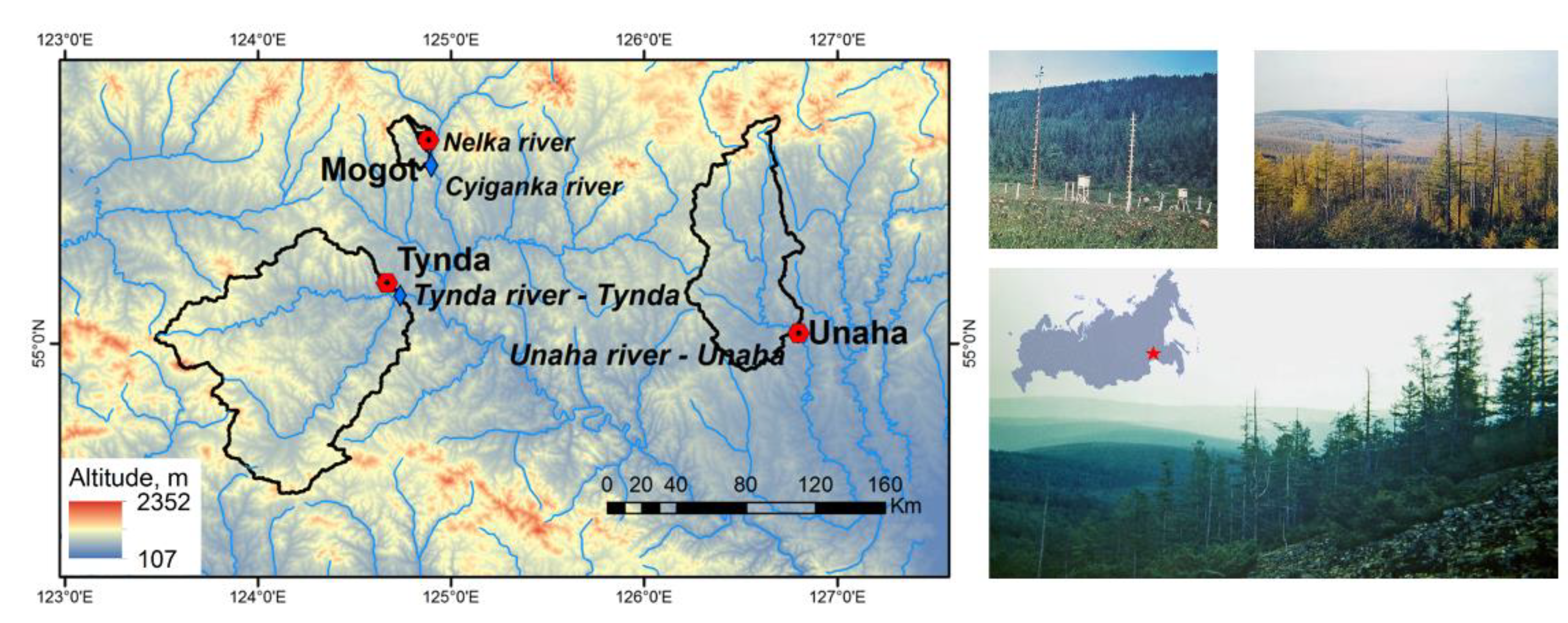
Figure 2.
The objects of the study.
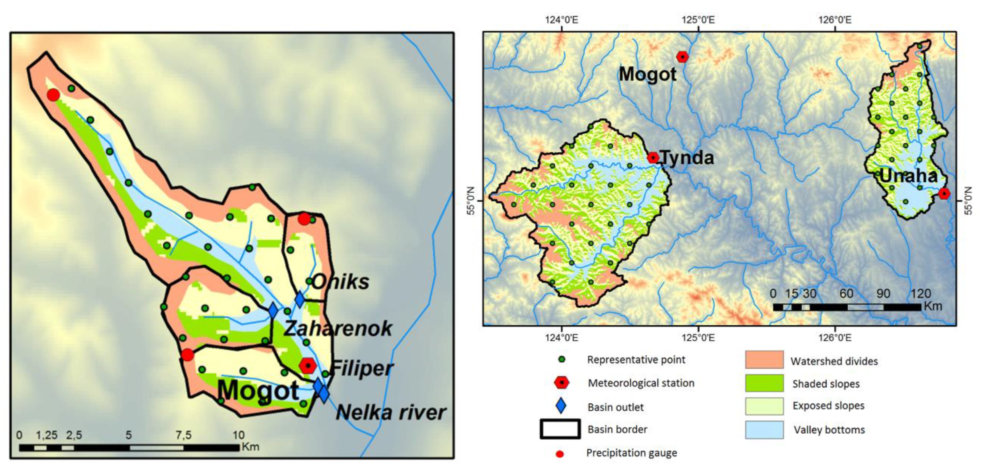
Figure 3.
Schematized soil columns.
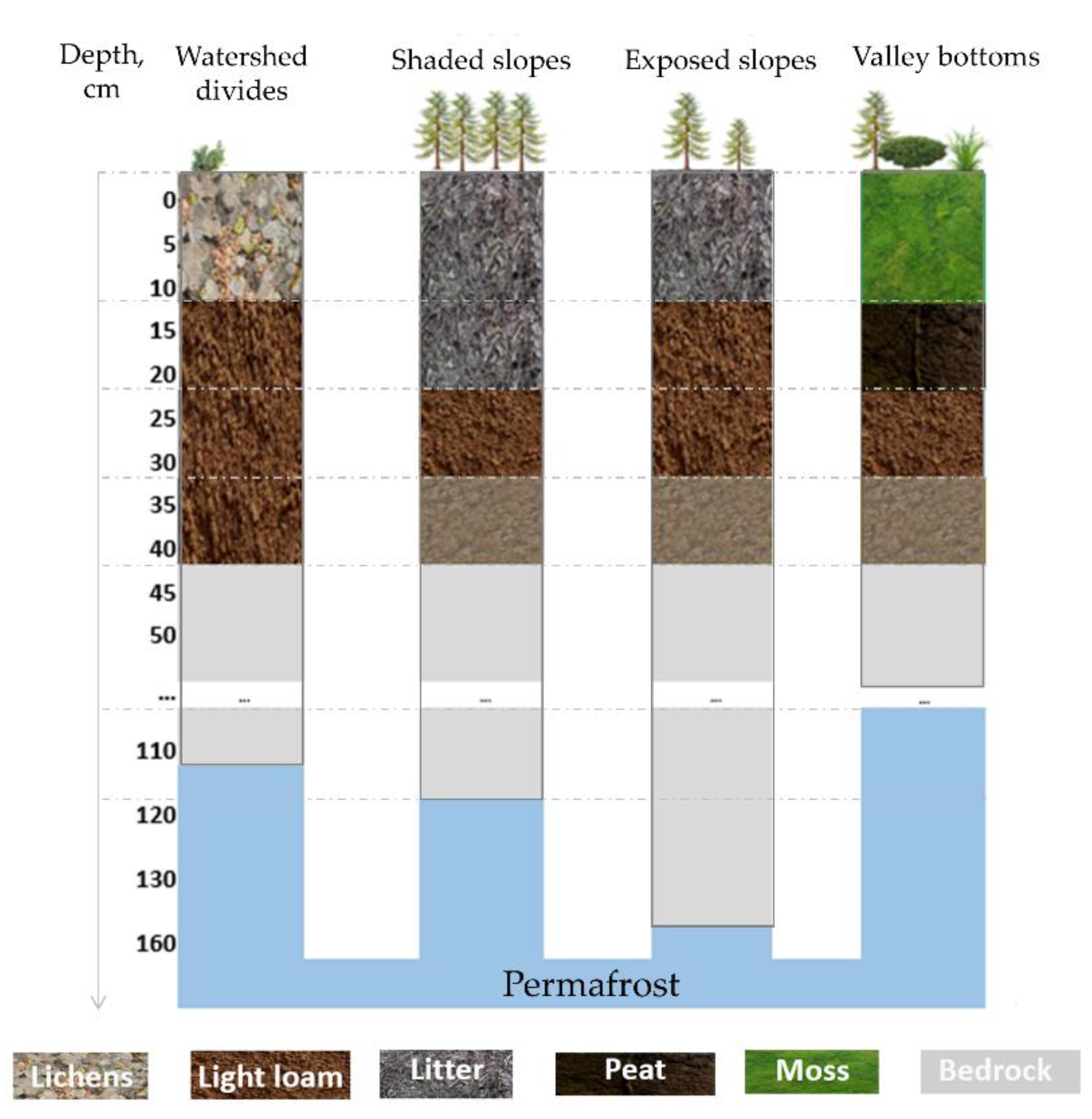
Figure 4.
Simulated and observed annual values of evaporation from snow (mm), 1980-1985.
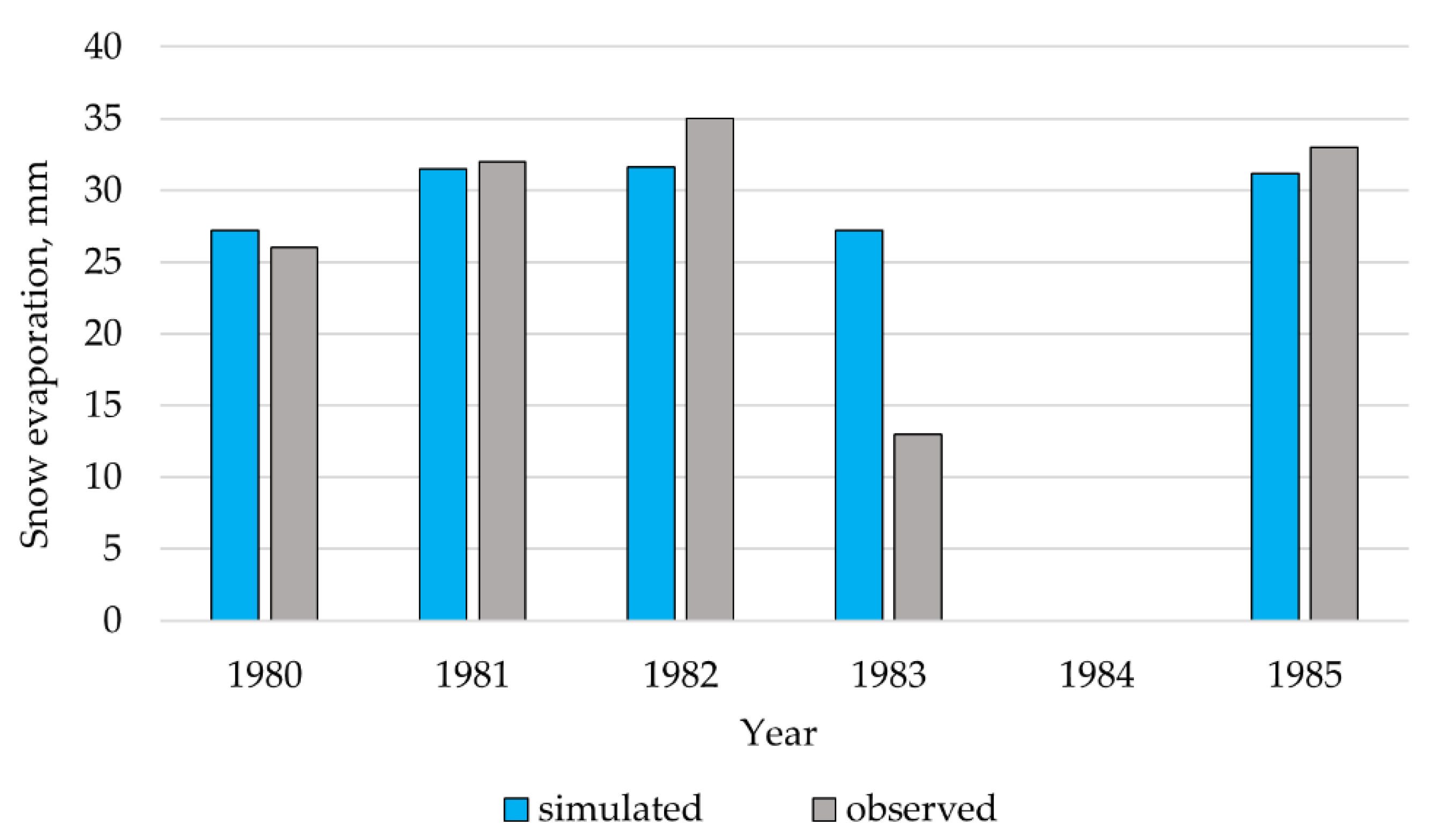
Figure 5.
Simulated and observed snow water equivalent (mm), 1981-1985.
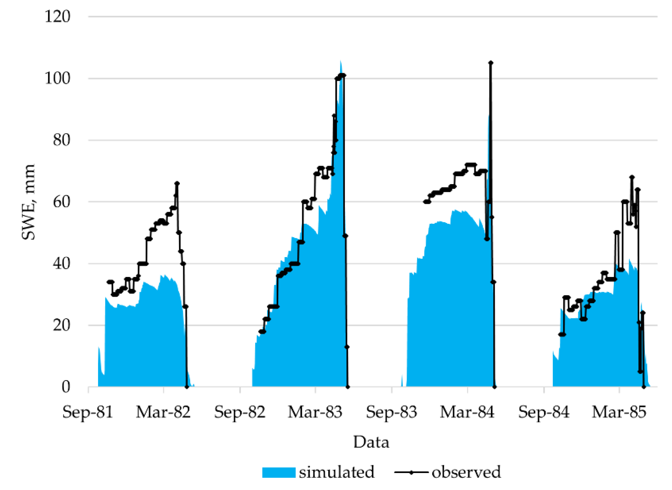
Figure 6.
Depth of soil thawing and soil freezing (m), 1980-1984.
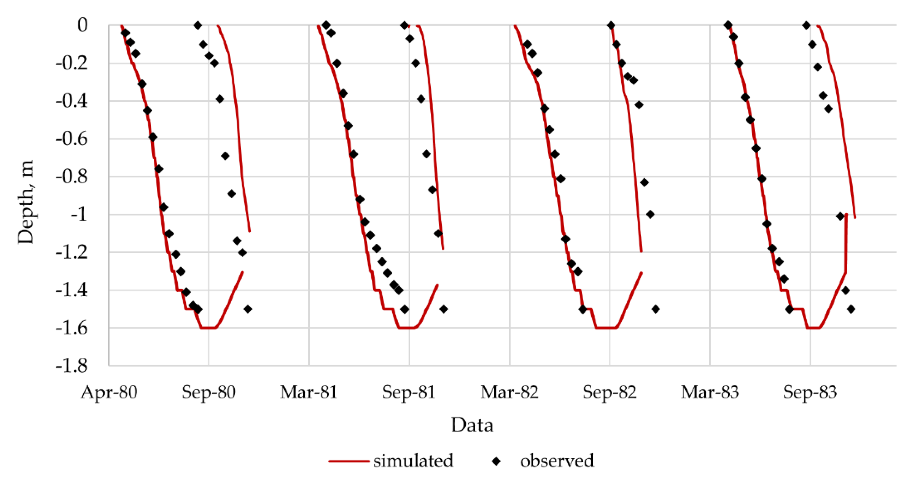
Figure 7.
Simulated and observed daily values of ground temperature (°C) at depths of 5, 50, 150 cm, 1980.
Figure 7.
Simulated and observed daily values of ground temperature (°C) at depths of 5, 50, 150 cm, 1980.
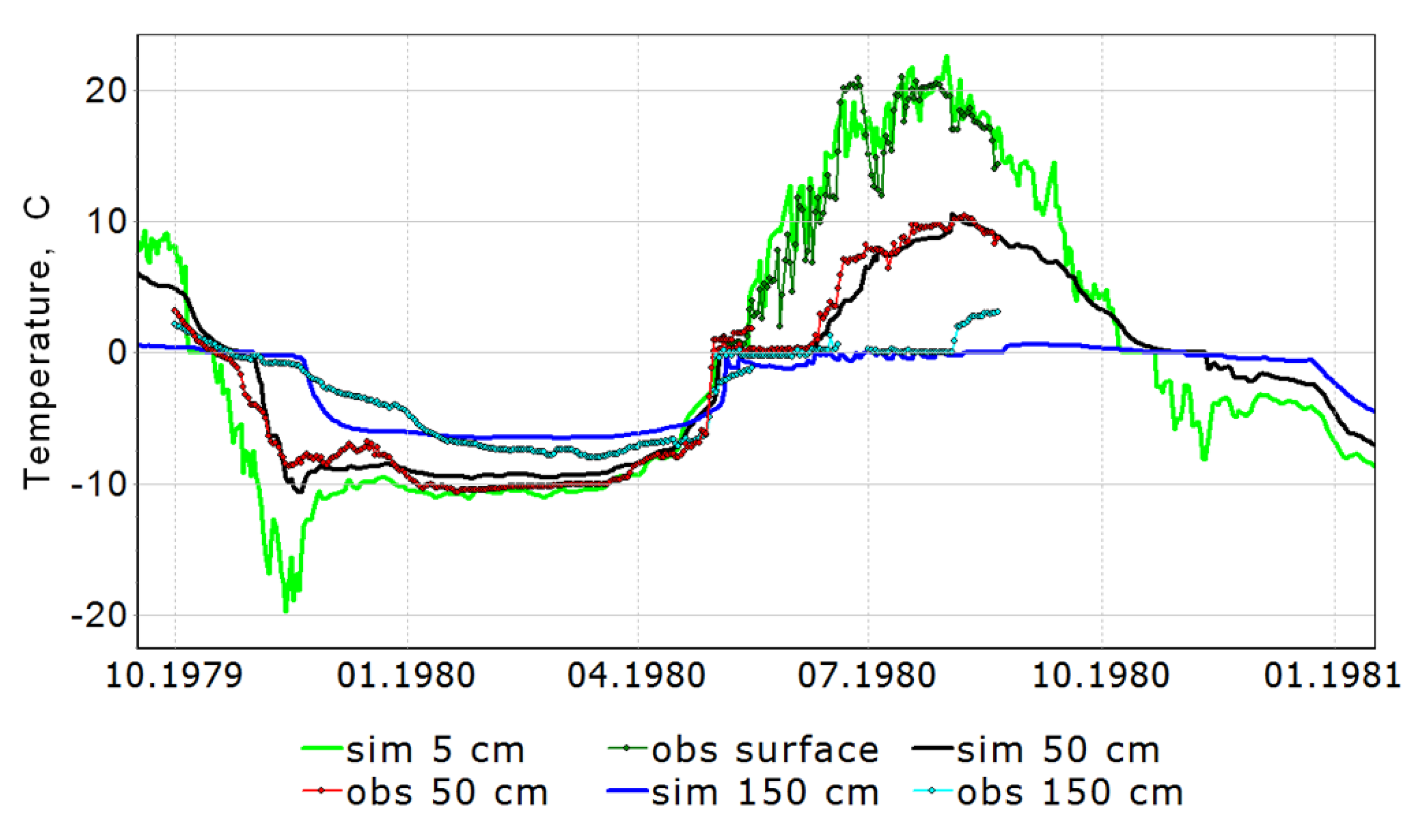
Figure 8.
Simulated and observed streamflow (m3/s) with high (1) and low (2) NS values: a – the Zakharenok stream (1978, 1977); b – the Filiper stream (1981, 1984); c – the Onyx stream (1979, 1985).
Figure 8.
Simulated and observed streamflow (m3/s) with high (1) and low (2) NS values: a – the Zakharenok stream (1978, 1977); b – the Filiper stream (1981, 1984); c – the Onyx stream (1979, 1985).
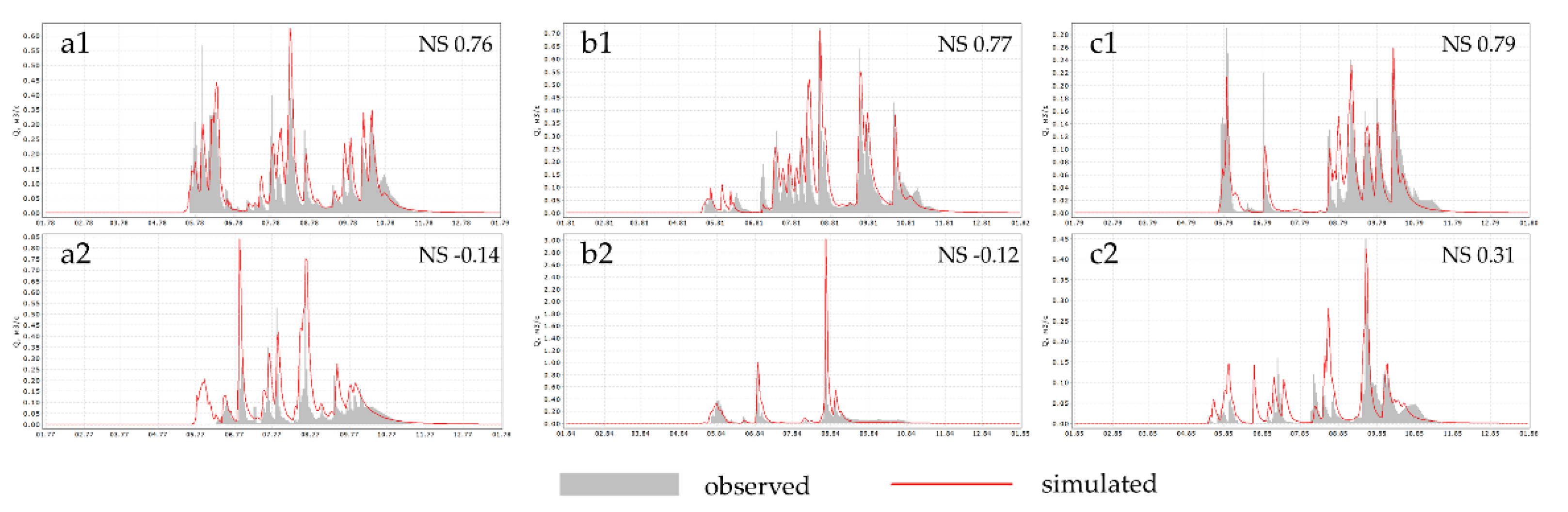
Figure 9.
Simulated and observed streamflow (m3/s) with high (1) and low (2) NS values: a – the Nelka River (1981, 1985); b – the Tsyganka River (1981, 1979).
Figure 9.
Simulated and observed streamflow (m3/s) with high (1) and low (2) NS values: a – the Nelka River (1981, 1985); b – the Tsyganka River (1981, 1979).
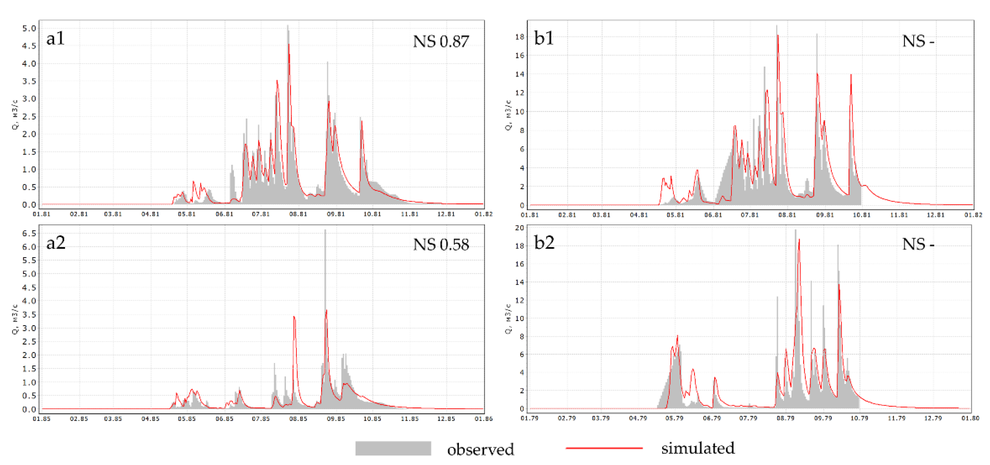
Figure 10.
Simulated and observed streamflow (m3/s) with high (1) and low (2) NS values: a – the Unakha River (1991, 1974); b – the Tynda River (1972, 2005).
Figure 10.
Simulated and observed streamflow (m3/s) with high (1) and low (2) NS values: a – the Unakha River (1991, 1974); b – the Tynda River (1972, 2005).
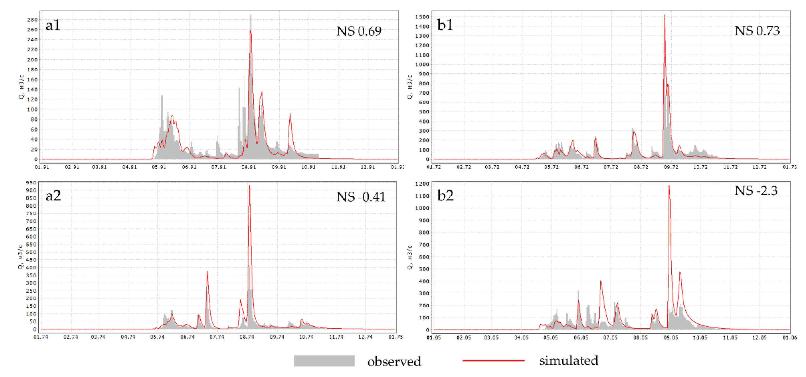

Table 1.
The hydrological gauges under study.
| Gauge | Catchment area, km2 | The average height of the catchment area, m | Length of the riverbed network, km | Average catchment slope, º/˚˚ |
|---|---|---|---|---|
| The Onyx stream | 3.0 | 780 | 2.0 | 190 |
| The Filiper stream | 4.7 | 710 | 5.1 | 147 |
| The Zakharyonok stream | 5.8 | 700 | 4.2 | 171 |
| The Nelka River | 30.8 | 850 | 27.0 | 170 |
Table 2.
Soil parameters.
| Soil parameters | The method of determining the parameter | Lichens | Plant litter | Moss | Light loam | Sandy loam | Peat |
|---|---|---|---|---|---|---|---|
| Density, kg/m3 | field | 1680 | 1300 | 520 | 2600 | 2600 | 1700 |
| Porosity, m3/ m3 | field | 0.87 | 0.92 | 0.90 | 0.60 | 0.35 | 0.83 |
| Maximum water holding capacity, m3/ m3 | field | 0.25 | 0.30 | 0.35 | 0.25 | 0.15 | 0.40 |
| Filtration coefficient, mm/min | field | 24 | 12 | 1.8 | 0.1 | 0.01 | 0.1 |
| Heat capacity, J /(kgºC) | assessment by soil type | 780 | 840 | 1930 | 830 | 830 | 1930 |
| Heat conductivity, W/(mºC) | assessment by soil type | 1.5 | 1.3 | 0.8 | 1.7 | 1.7 | 0.8 |
| Hydraulic parameter, m3/s | expert assessment, calibration |
The active layer Top organic layer: 10 Lower mineral layer: 0.005 |
|||||
Table 3.
The main results of hydrological modeling.
| Gauges | Period | Yo | Ys | P | E | Qo | Qs | NS (m/av) |
NS (max, гoд) |
NS (min, гoд) |
| Onyx stream | 1976-1985 | 243 | 342 | 607 | 259 | 0.66 | 1.20 | 0.65/0.64 | 0.79(1979) | 0.31(1985) |
| Filiper stream | 1976-1985 | 255 | 346 | 634 | 285 | 1.37 | 3.02 | 0.55/0.40 | 0.77(1981) | -0.12(1984) |
| Zakharyonok stream | 1976-1985 | 216 | 363 | 628 | 260 | 1.51 | 2.88 | 0.35/0.26 | 0.76(1978) | -0.14(1977) |
| Nelka River | 1976-1985 | 295 | 323 | 658 | 327 | 9.73 | 15.2 | 0.71/0.70 | 0.87(1981) | 0.58(1985) |
| Tsyganka River | 1976-1985 | - | 308 | 617 | 306 | - | - | - | - | - |
| Unakha River - Unakha | 1966-1994 | 327 | 342 | 640 | 300 | 875 | 456 | 0.46/ 0.40 | 0.69(1991) | -0.41(1974) |
| Tynda River - Tynda | 1966-2012 | 286 | 293 | 645 | 354 | 1450 | 2500 | 0.52/0.31 | 0.73(1972) | -2.3(2005) |
where Yo and Ys are the observed and calculated average annual streamflow, mm; P is precipitation, mm; E is evaporation, mm; Qo and Qs are the maximum observed and calculated discharges, m3/s; m and av NS are the median and average NS; max and min NS is the maximum and minimum value of NS.
Disclaimer/Publisher’s Note: The statements, opinions and data contained in all publications are solely those of the individual author(s) and contributor(s) and not of MDPI and/or the editor(s). MDPI and/or the editor(s) disclaim responsibility for any injury to people or property resulting from any ideas, methods, instructions or products referred to in the content. |
© 2024 by the authors. Licensee MDPI, Basel, Switzerland. This article is an open access article distributed under the terms and conditions of the Creative Commons Attribution (CC BY) license (http://creativecommons.org/licenses/by/4.0/).
Copyright: This open access article is published under a Creative Commons CC BY 4.0 license, which permit the free download, distribution, and reuse, provided that the author and preprint are cited in any reuse.


