Submitted:
10 December 2024
Posted:
11 December 2024
You are already at the latest version
Abstract
We consider temporal optical effects in the presence of static fields, and more general, in anisotropic optical materials. We show that magneto-optical effects can occur due to temporal variations of the refractive index. Faraday rotations, Cotton-Mouton effects and other polarimetric processes due to static magnetic or electric fields are demonstrated. Exemples of magneto-plasmas and nonlinear Kerr media are discussed in detail. These temporal processes could be of general interest in photonics.
Keywords:
temporal optics
; Faraday rotation
; Kerr media
; plasmas
; magneto-optics
1. Introduction
Temporal effects in optical media have received considerable attention in recent years [1,2,3], and the area of spacetime optics has shown a considerable growth (see the reviews [4,5]). Several different temporal processes and configurations have been considered, including time-refraction and time-reflection [6,7], temporal beam-splitters [8,9], photon acceleration [10,11,12], spatiotemporal Bragg gratings [13] and the related problem of time-crystals [14,15,16,17], light amplification [17,18], temporal quantum optics [19,20,21,22] with direct extensions to electron QED [23,24], time-varying metamaterials [25,26,27], as well as negative refraction in epsilon near-zero systems [28,29]. Quite recently, the case of Faraday rotations induced by a temporal interface has been studied [30].
In this paper, we return to the case of temporal Faraday effect, and examine the more general problem of temporal magneto-optics. We show that Faraday rotation cannot be observed with a single temporal interface, and that a sequence of two opposite temporal interfaces is needed. We show that, not only Faraday rotation but also a Cotton-Mouton type of ellipticity can be induced by temporal processes in birefringent media. Polarization rotation and induced ellipticity result from two different temporal processes, which are wave amplification and birefringent frequency shifts.
The paper content is the following. First, in Section 2, we consider a single temporal interface that we describe as a time-refraction process. We show that, in this case, no Faraday rotation can be observed. In Section 3, we examine the restored frequency shifts that result from two consecutive temporal interfaces with opposite sign, and calculate the resulting Faraday rotation, for transmitted and reflected waves. In Section 4, we consider two specific physical situations. The first is wave propagation in a non-stationary plasma. We calculate the temporal Faraday effect that can be observed for wave propagation along the direction of a static magnetic field . Similar effects persist for oblique propagation, and the Cotton-Mouton effect is discussed for perpendicular propagation. The other example is related with a nonlinear optical medium, which exhibits Kerr birefringence. This example is analogous to the Couton-Mouton effect, in the sense that it only envolves no ellipsometric changes, and no polarization rotation is observed. In Section 5, we examine the more general situation where the sharp temporal interfaces are replaced by arbitrary temporal changes of the optical medium. We demonstrate that, even in this case, temporal magneto-optical can still be observed, as long as the temporal changes are temporally symmetric, and bring the medium to its initial state. Finally, in Section 6, we state some conclusions.
2. Single Temporal Interface
We consider an optical medium with an axis of symmetry, for instance , a static magnetic field . We assume a wave propagating along some direction, with wavevector and frequency , before entering the anisotropic medium, as described by the electric field
where represent two orthogonal modes (not only right and left-hand circular polarization, but also linear orthogonal modes, according to the physical situation), and
where the amplitudes and correspond to modes with same wavenumber and frequency , but propagating in opposite directions. As initial conditions, at , we assume a linear field polarization along some direction defined by the unit vector , such that
To be more specific, let us assume propagation along the z-axis, using , parallel to the static magnetic field . For linear polarization at an angle from the x-axis, we can write the unit polarization vector as
where represent the left and right-hand unit vectors, as . We then assume a sudden change of the refractive index of the medium , occurring at , such that, for invariant , we have a frequency shift determined by
It is well-known that, in order to satisfy the validity of Maxwell’s equation for all times, the fields have to satisfy the continuity conditions
for , where the displacement and magnetic fields are related with the wave electric field by the relations
and is the dielectric tensor. This allows us to write for each wavevector component of the spectrum, valid for , the following wave amplitude relations:
and
It is now useful to define the parameters
which allow us to write the amplitude relations
We can then obtain the transmission and reflection coefficients, for each polarization state, and , as
and
They are sometimes called the temporal Fresnel formulae, and correspond to a straightforward generalization of previous results [8,21]. We notice that they depend on the ratio between the initial amplitudes for propagating and counter-propagating modes, , which clearly indicate that this is a linear four-wave mixing process. We also notice that, at this point we cannot talk about a total field polarization state, because for each mode oscillates with different frequencies, . We simply have two independent modes, with two different polarizations and frequencies, where the total field associated with the wavevector is determined by the sum of these two modes, as
with
where .
3. Restored Frequency
In order to consider possible polarimetric effects on a single wave mode, we need a process that could restore the initial frequency, . This can be done using a second temporal boundary with the opposite sign, occurring at some later time , where the refractive index returns to its initial value: . These two consecutive temporal boundaries define what could be called a temporal beam-splitter [8].
It is particularly useful to derive the final transmission and reflection coefficients, and , resulting from this temporal beam-splitter in the presence of birefringence effects. For this purpose, we take the particular case of . Using eqs. (12)-(13), the fields at will the be determined by
and
where . This simplifies to
and
This means that the total fields of the mode , coming out of the temporal beam-splitter is
This is to be compared with the initial field (1)-(2). In particular, it means that the total transmitted field is determined by
where we have used a simplified notation, which has to be compared with
This shows that three different effects were introduced by the temporal beam-splitter: i) field amplification, due to the factors ; ii) rotation of the polarization direction; iii) creation of ellipticity. The first effect already exists in isotropic media. The other two are due to anitropy, and will be illustrated next. To understand them, we write eq. (18) in the form
with
and
Similarly, for the reflected wave, we would get
to be compared with . The amplitudes of the above transmission and reflection coefficients oscillate as a function of the temporal width , as in the case of the usual spatial beam-splitter. This clearly shows the existence of temporal interferences, different for each mode, as illustrated in Figure 1. The above results are applied to specific physical situation on the next section, where temporal processes in the presence of static magnetic and electric fields will be considered.
4. Specific Examples
4.1. Magnetized Plasmas
As a first example, let us consider a plasma in a static magnetic field. We assume that the plasma is suddenly created at time , and vanishes at time . We assume the most interesting case of parallel propagation, and take . Alternatively, we could assume the sudden creation of a (quasi) static magnetic field in a pre-created plasma, but the physical conditions would be more difficult to define. The eigen-modes ± can therefore be identified with right and left-hand circularly polarized modes [31]. This leads to
where is the electron plasma frequency, and is the electron cyclotron frequency. For a given initial frequency , we get
These new frequencies are therefore determined by the equation
We can see that the frequency shift can be very strong when we approach the resonant frequency for one of the modes, . Strong effects can also be expected near a cutoff, when . In both situations, we can have . Here we disregard such critical situations and use, for illustration, the case of very high frequencies, such that . In this case, we expect very small frequency shifts, , as determined by the approximate solution
We can then calculate the final rotation of the electric polarization state, valid for , as determined by the above expressions for the transmission and reflection coefficients. This leads to
where we have used the phases given by
and
This is illustrated numerically on Figure 2, where the initial and final polarisation states are linear. We can then state that a temporal beam-splitter in a plasma produces an effect similar to the well-known Faraday effect, which is due to the presence of a static magnetic field parallel to the propagation direction.
On the same figure, we also represent the electric field direction inside the temporal beam-splitter, for , before taking the final form. the observed oscillations are partly due to the difference between the two mode frequencies . During this time interval, we have two distinct frequency modes with circular polarization turning in opposite directions, but we can only talk about a polarization rotation after , when the wave emerges from the temporal beam-splitter with the original frequency .
This magneto-optic effect is not limited to parallel propagation, because two orthogonal polarization states exist in a plasma, for high frequency waves propagating along any direction with respect to the static magnetic field. In particular, for wave propagation in a direction perpendicular to , the two eigen-modes correspond to linear polarization, parallel and perpendicular to the static field. In this case, we should replace the previous notation by a more appropriate notation . Using, once more the cold plasma model, we can specify these new modes by the dielectric functions [31]
where is the upper-hybrid frequency. The frequency shifts observed inside the temporal beam-splitter are now given by
which are formally identical to eq. (28). This would lead to a change in ellipticity, a characteristic feature of the Cotton-Mouton effect. There is a small problem related to the field continuity relations. A longitudinal field component is needed to define the complete state of the perpendicular wave mode, which is absent before the first temporal boundary, as well as after the second one. However, the longitudinal field component is immediately established in the plasma, in response to the transverse component, because of the negligible electron inertia [30].
4.2. Nonlinear Kerr Medium
Another important example is related to a nonlinear optical medium, and not a plasma. We consider a generic Kerr medium, where the optical birefringence is associated to a static electric field , instead of a static magnetic field. This case is similar to the above, with two linearly polarized eigen-modes, but where now the static field modifies the refractive index of the parallel polarization, not the perpendicular one. Instead of eq. (34), we then have [32]
where is the wavelength, is the linear susceptibility, and is a characteristic constant of the optical material. An increase of the refractive index will induce a down-shift of the parallel frequency mode , as given by
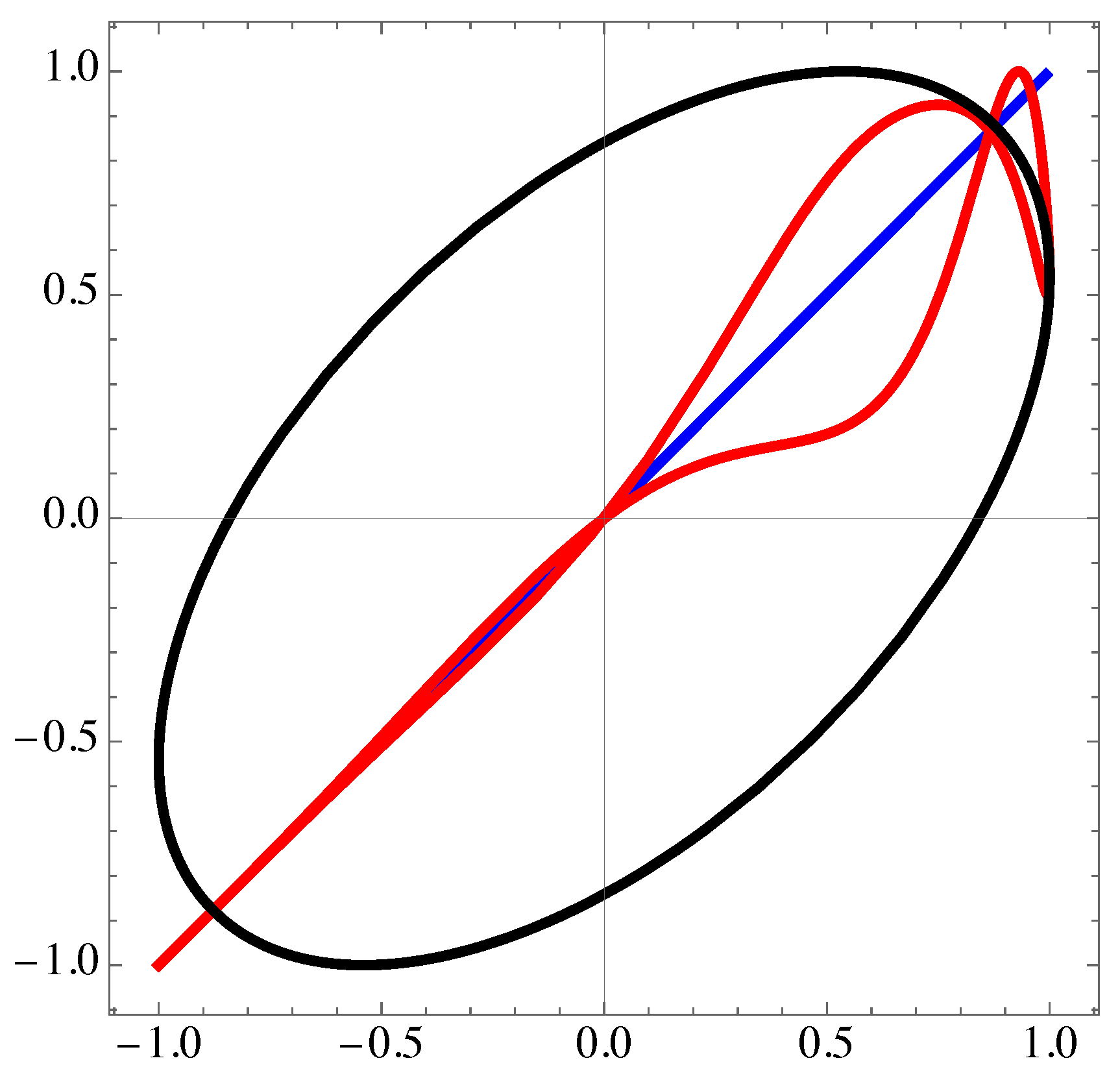
This leads to a change in the polarization ellipticity, and not a rotation, as illustrated in Figure 3. For an initial state of linear polarization, we obtain at the end of the temporal beam-splitter an elliptic polarization, very similar to what would occur in the Cotton-Mouton effect.
5. Slow Time Variations
It is well-known that the temporal discontinuities discussed above are only valid for temporal changes that occur on a time-scale much shorter than the wave period. This is, in general, very difficult to achieve. We therefore need to extend our discussion the case of arbitrary temporal variations of medium. This can be described by a sequence of infinitesimal time steps, from t to [33]. Let us then assume that the refractive index of the medium is described by a continuous function of time, , to be specified. In analogy with eq. (1), let us consider the total electric field associated with a given wavevector component , as
with
But, in contrast with eq. (2), where the field amplitudes were assumed constant, the new field amplitudes and are now slowly varying functions of time, which evolve on a time-scale much longer than the wave period, and the phase functions are defined by
where is the initial time, and are the time-varying mode frequencies. Applying the approach of [33] for each mode, it is then possible to show that the field amplitudes evolve as
and
with
These equations can be formally solved [12]. But, for the present purposes, it is useful to consider the plausible case of very weak reflected waves, where we have , we can use the approximate expressions
and
This leads to simple expressions for the transmission and reflection coefficients, as given by
and
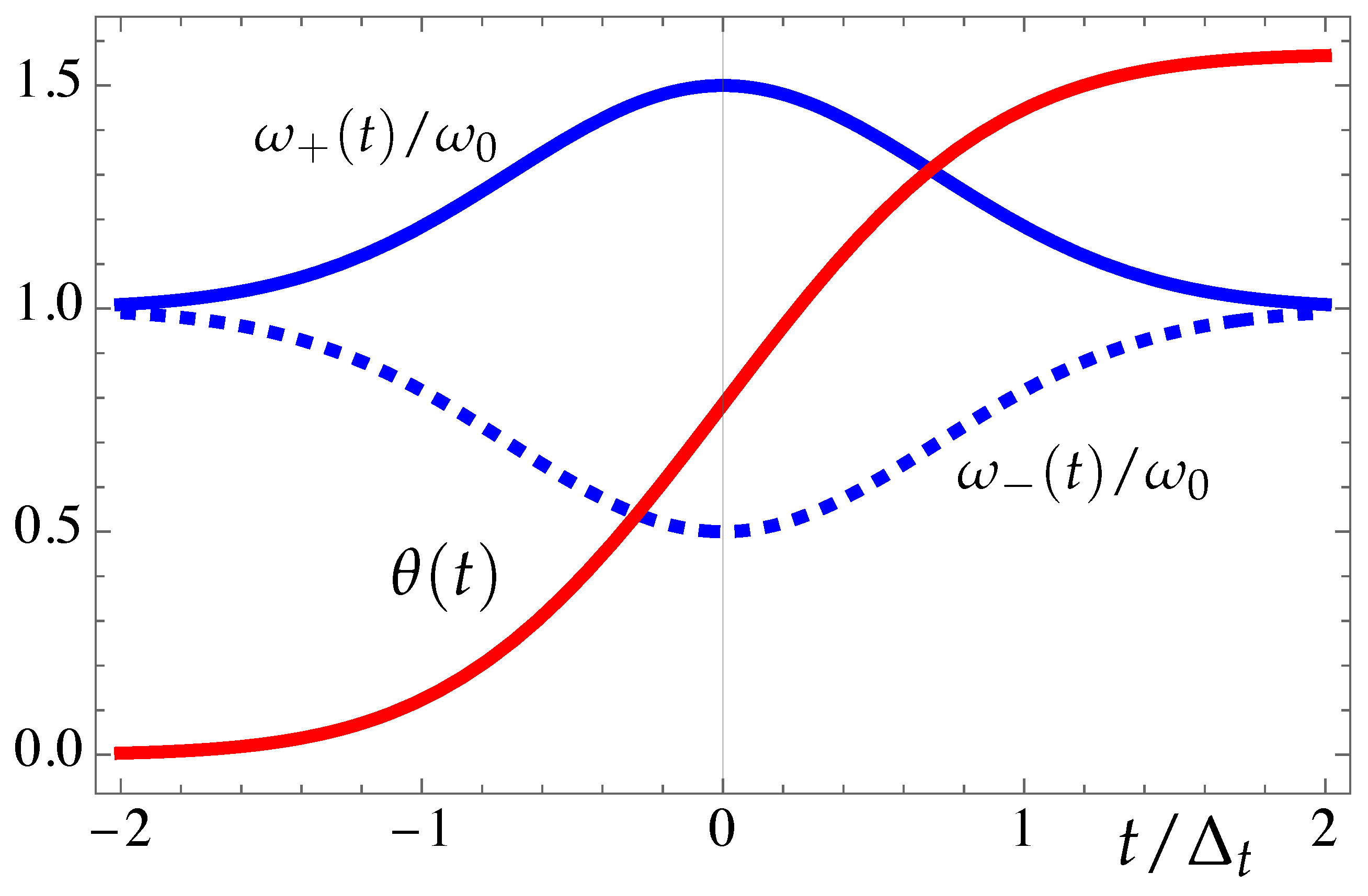
As an illustrative example, we consider the case of a magneto-plasma, assuming a constant magnetic field, , and a plasma density evolving as as Gaussian function, with a typical duration of . We can write
where is the maximum value of the plasma frequency. For parallel propagation, this leads to approximate values of the circularly polarized eigen-mode frequencies, determined by
where we have used the initial wave frequency , and the auxiliary frequency . This leads to
These expreesions can be used to calculate the coefficients (46) and (47). Let us focus on the transmission coefficient. We have
We can see that, for , the asymptotic value of tends to one, and the reflection coefficient becomes zero. However, even in the unfavourable of , temporal Faraday rotation still exists because of the frequency difference between the two modes. The total phase-shift resulting from such difference is given by
This is illustrated in Figure 4.
If, instead of circularly polarized eigen-modes we have two linearly polarized modes, as in the nonlinear Kerr effect, the temporal transmission coefficients in this approximation will be , and
where , and is the static electric field. Again, this leads to . Still, in this case, a final frequency shift between the two linear modes remains, due to the different frequencies, leading to a final change of ellipticity. This means that, in all cases, with or without temporal amplification, a temporal beam-splitter with arbitrary temporal profile always leads to magneto-optical effects.
6. Conclusions
In this paper, we have studied the magneto-optical effects, such as Faraday rotation and similar processes, resulting from reversible temporal perturbations of a birrefringent medium. These perturbations were described as temporal beam-splitters, using sharp temporal boundaries, as well as slowly varying boundaries described by a Gaussian function. The cases of a cold magnetized plasma, and nonlinear Kerr media were examined in detail.
We have shown that two different processes contribute to these magneto-optical effects. One is an eventual wave amplification resulting from the influence of a temporal beam-splitter, where the transmission coefficients can be significantly larger than one. This is particularly important for sharp boundaries. The other is the phase-shift between the two eigen-modes, which is always present. In the case of a Faraday rotation, these eigen-modes correspond to left and right-hand polarization, propagating along the static magnetic field. In the case of Cotton-Mouton and nonlinear Kerr effects, the two eigen-modes are linearly polarised, and propagate across the static magnetic or electric fields.
We were able to demonstrate that these effects can be observed in a variety of physical situations and in different anisotropic media, such as a plasma or a nonlinear Kerr optical medium, where the anisotropy is due to the presence of a static electric or magnetic field. They could eventually be used to develop new configurations in spacetime optics, as well as in diagnostics of ultrashort laser pulses.
References
- Plansinis, B.W.; Donaldson, W.R.; Agrawal, G.P. "What is the Temporal Analog of Reflection and Refraction of Optical Beams? ", Phys. Rev. Lett. 2015, 115, 183901. [Google Scholar] [CrossRef]
- Biancalana, F.; Amann, A.; Uskov, A.V.; O’Reilly, E.P. "Dynamics of Light Propagation in Spatiotemporal Dielectric Structures", Phys. Rev. E 2007, 75, 046607. [Google Scholar]
- Mendonça, J.T.; Shukla, P.K. "Time Refraction and Time Reflection: Two Basic Concepts", Phys. Scripta 2002, 65, 160. [Google Scholar] [CrossRef]
- Galiffi, E.; Tirole, R.; Yin, S.; Li, H.; Vezzoli, S.; Huidobro, P.A.; Silveirinha, M.G.; Sapienza, R. ; AlùA. ; Pendry, J.B. "Photonics of Time-Varying Media", Adv. Photonics 2022, 4, 014002. [Google Scholar]
- Mendonça, J.T. "Time Refraction and Spacetime Optics", Symmetry 2024, 16, 1548.
- Moussa, H.; Xu, G.; Yin, S.; Galiffi, E.; Radi, Y.; Alú, A. "Observation of Temporal reflection and Broadband Frequency Translation at Photonic Time Interfaces", Nature Phys. 2023, 19, 863.
- Lustig, E.; Segal, O.; Saha, S.; Bordo, E.; Chowdhury, S.N.; Sharabi, Y.; Fleischer, A.; Boltasseva, A.; Cohen, O.; Shalaev, V.M.; Segev, M. "Time-refraction optics with single cycle modulation", Nanophotonics 2023, 12, 2221.
- Mendonça, J.T.; Martins, A.M.; Guerreiro, A. "Temporal Beam Splitter and Temporal Interference", Phys. Rev. A 2003, 68, 043801. [Google Scholar] [CrossRef]
- Rizza, C.; Castaldi, G.; Galdi, V. "Short-Pulsed Metamaterials", Phys. Rev. Lett. 2022, 128, 257402. [Google Scholar] [CrossRef]
- Sandberg, R.T.; Thomas, A.G.R. "Photon Acceleration from Optical to XUV", Phys. Rev. Lett. 2023, 130, 085001. [Google Scholar] [CrossRef]
- Shcherbakov, M.R.; Werner, K.; Fan, Z.; Talisa, N.; Chowdhury, E. ; Shvets,G. "Photon Acceleration and Tunable Broadband Harmonics Generation in Nonlinear Time-dependent Metasurfaces", Nat. Commun. 2019, 10, 1345. [Google Scholar]
- Mendonça, J.T. "Photon Acceleration by Superluminal Ionization Fronts", Symmetry 2024, 16, 112.
- J. Zhang, J.; W.R. Donaldson, W.R.; and G.P. Agrawal, G.P. "Spatiotemporal Bragg gratings forming inside a nonlinear dispersive medium", Opt. Lett. 2024, 49, 5854.
- Lustig, E.; Segal, O.; Saha, S.; Fruhling, C.; Shalaev, V.M.; Boltasseva, A.; Segev, M. "Photonic time- crystals - fundamental concepts," Optics Express 2023, 31, 9165.
- Wang, X.; Mirmoosa, M.S.; Asadchy, V.S.; Rockstuhl, C.; Fan, S.; Tretyakov, S. “Metasurface-based realization of photonic time crystals,” Sci. Adv. 2023, 9, eadg7541 (2023).
- Sacha, K.; Zakrzewski, J. "Time Crystals: a review", Rep. Prog. Phys. 2018, 81, 016401. [Google Scholar] [CrossRef]
- Lyubarov, M.; Lumer, Y.; Dikopoltsev, A.; Lustig, E.; Sharabi, Y.; Segev, M. "Amplified Emission and Lasing in Photonic Time Crystals", Science 2022, 377, 425.
- Horsley, S.A.R.; Pendry, J.B. "Traveling Wave Amplification in Stationary Gratings", Phys. Rev. Lett. 2024, 133, 156903. [Google Scholar] [CrossRef]
- Svidzinsky, A. "Time Reflection of Light from a Quantum Perspective and Vacuum Entanglement", Opt. Express 2024, 32, 15623. [Google Scholar] [CrossRef]
- Prain, A.; Vezzoli, S.; Westerberg, N.; Roger, T.; Faccio, D. "Spontaneous Photon Production in Time-dependent Epsilon-near-zero Materials", Phys. Rev. Lett. 2017, 118, 133904. [Google Scholar] [CrossRef]
- Mendonça, J.T.; Guerreiro, A.; Martins, A.M. "Quantum Theory of Time Refraction", Phys. Rev. A 2000, 62, 033805. [Google Scholar] [CrossRef]
- Dodonov, V.V.; Klimov, A.B.; Nikonov, D.E. "Quantum Phenomena in Nonstationary Media", Phys. Rev. A 1993, 47, 4422. [Google Scholar] [CrossRef]
- Ok, F.; Bahrami, A.; Caloz, C. "Electron Scattering at a Potential Temporal Step Discontinuity", Sci. Rep. 2024, 14, 5559. [Google Scholar]
- Mendonça, J.T. "Particle-Pair Creation by High-Harmonic Laser Fields", Phys. Scr. 2023, 98, 125606. [Google Scholar]
- Engheta, N. "Four-dimensional optics using time-varying metamaterials", Science 2023, 379, 1190.
- Yuan, L. ; Fan,S. "Temporal Modulation Brings Metamaterials Into New Era", Light Sci. Appl. 2022, 11, 173. [Google Scholar]
- Caloz, C.; Deck-Léger, Z.-L. “Spacetime metamaterials” IEEE Trans. Antennas Propag. 2019, 67, 1569. [Google Scholar]
- Bruno, V.; DeVault, C.; Vezzoli, S.; Kudyshev, Z. et al. , "Negative Refraction in Time-Varying Strongly Coupled Plasmonic-Antenna Epsilon Near-Zero Systems", Phys. Rev. Lett. 2020, 124, 043902. [Google Scholar]
- Zhou, Y.; Alam, M.Z.; Karimi, M.; Upham, J.; Reshef, O.; Liu, C.; Willner, A.E. ; Boyd,R. W. "Broadband Frequency Translation Through Time Refraction in an Epsilon-Near-Zero Material", Nat. Commun. 2020, 11, 2180. [Google Scholar]
- Li, H.; Yin, S. ; and Alú,A. "Nonreciprocity and Faraday Rotation at Time Interfaces", Phys. Rev. Lett. 2022, 128, 173901. [Google Scholar]
- Swanson, D.G. Plasma Waves, (2nd ed.), Institute of Physics Publishing: Bristol, 2003.
- Landau, L.D.; Lifshitz, E.M.; Pitaevskii, L.P. Electrodynamics of Continuous Media, Vol. 8 (2nd ed.). Butterworth-Heinemann: Oxford, 1984.
- Mendonça, T.T.; Guerreiro, A. "Time refraction and the quantum properties of vacuum", Phys. Rev. A 2005, 72, 063805. [Google Scholar] [CrossRef]
Figure 1.
(blue curves) and (red curves): as a function of , for and (dashed).
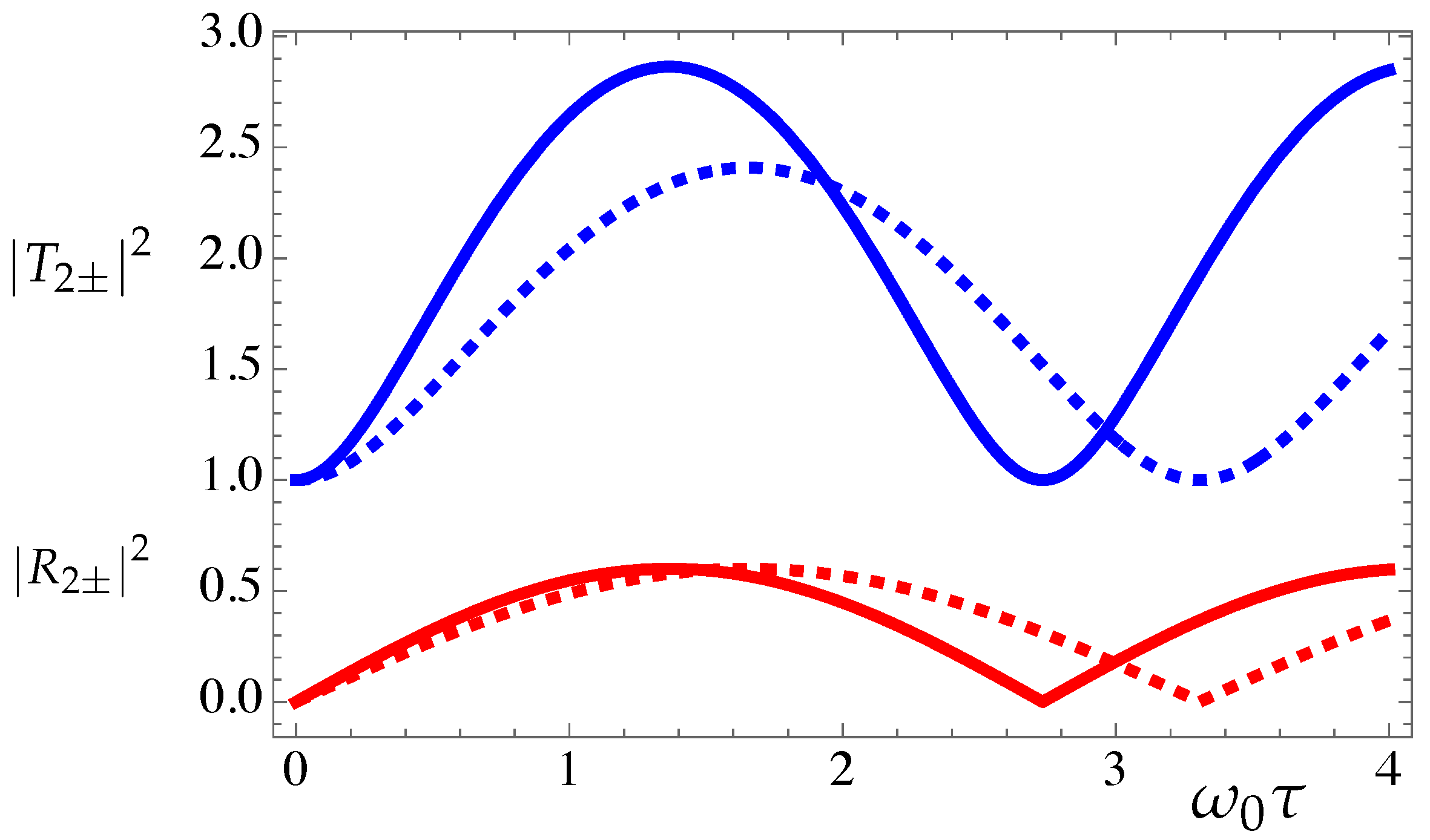
Figure 2.
Faraday rotation: transverse plane of polarization, showing rotation of the linear polarization. Initial state (in blue) and the final state (in black), when we assume . Also represented a the more accurate result with (in black, dashed). The electric field direction follows a complicated pattern inside the temporal beam-splitter, as shown in red, before taking the final form.
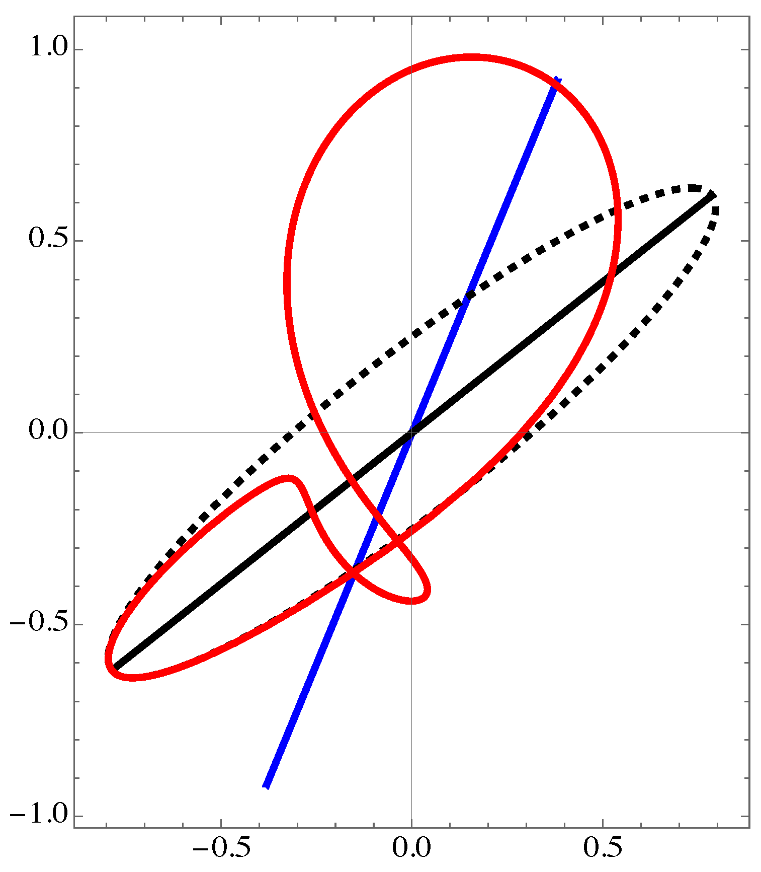
Figure 3.
Nonlinear Kerr effect: Transverse plane of polarization, representing the initial linear polarization (in blue) and the final elliptic state (in black). The electric field direction inside the temporal beam-splitter is illustrated by the curve in red.
Figure 3.
Nonlinear Kerr effect: Transverse plane of polarization, representing the initial linear polarization (in blue) and the final elliptic state (in black). The electric field direction inside the temporal beam-splitter is illustrated by the curve in red.
Disclaimer/Publisher’s Note: The statements, opinions and data contained in all publications are solely those of the individual author(s) and contributor(s) and not of MDPI and/or the editor(s). MDPI and/or the editor(s) disclaim responsibility for any injury to people or property resulting from any ideas, methods, instructions or products referred to in the content. |
© 2024 by the authors. Licensee MDPI, Basel, Switzerland. This article is an open access article distributed under the terms and conditions of the Creative Commons Attribution (CC BY) license (http://creativecommons.org/licenses/by/4.0/).
Copyright: This open access article is published under a Creative Commons CC BY 4.0 license, which permit the free download, distribution, and reuse, provided that the author and preprint are cited in any reuse.


